Chiral edge soliton in nonlinear Chern systems

Abstract

We study the effect on the chiral edge states by including a nonlinearity to a Chern insulator which has two chiral edge states with opposite chiralities. We explore a quench dynamics by giving a pulse to one site on an edge and analyzing the time evolution of a wave packet. Without the nonlinearity, an initial pulse spreads symmetrically and diffuses. On the other hand, with the nonlinearity present, a solitary wave is formed by the self-trapping effect of the nonlinear term and undergoes a unidirectional propagation along the edge, which we identify as a chiral edge soliton. A further increase of the nonlinearity induces a self-trapping transition, where the chiral wave packet stops its motion. It is intriguing that the nonlinearity is controlled only by changing the initial condition without changing a sample.

Introduction: Topological physics is one of the most active fields in condensed matter physics, which  has been applied to photonic Raghu ; Hafe2 ; Hafezi ; KhaniPhoto ; WuHu ; TopoPhoto ; Ozawa16 ; Ley ; KhaniSh ; Zhou ; Jean ; Ota18 ; Ozawa ; Ota19 ; OzawaR ; Hassan ; Ota ; Li ; Yoshimi ; Kim ; Iwamoto21 , acousticProdan ; TopoAco ; Berto ; Xiao ; He ; Abba ; Xue ; Ni ; Wei ; Xue2 , mechanicalLubensky ; Chen ; Nash ; Paul ; Sus and electric circuitTECNature ; ComPhys ; Hel ; Lu ; YLi ; EzawaTEC ; EzawaLCR ; EzawaSkin systems. The Su-Schrieffer-Heeger (SSH) modelMalko ; XiaoSSH ; Jean ; Parto and the Chern insulatorRaghu ; Hafe2 ; Hafezi are realized in these systems. Nonlinear topological physics is an emerging field, which is also studied in photonicLey ; Zhou ; MacZ ; Smi ; Tulo ; Kruk ; NLPhoto ; Kirch ; TopoLaser , mechanicalSnee ; PWLo ; MechaRot ; Sin , electric circuitHadad ; Sone ; TopoToda and resonatorZange systems. The nonlinear term is typically introduced by the Kerr effect in photonicsChris ; Szameit . The system is described by the nonlinear Schrödinger equation. The simplest model is the nonlinear SSH modelZhou ; Gor ; Hadad ; Tulo ; Dob ; NLPhoto .

A soliton is a stable wave packet in nonlinear systems. Edge solitons are fascinating objectsLey ; Muk ; ZhangSoliton propagating along an edge of a sample. Solitons are often described by exact solutions in continuum theory. However, there seems to be no exact solutions in lattice systems due to the lack of the continuous translational symmetry in general.

The study of quench dynamics is a powerful method to reveal the essence of nonlinear topological systemsTopoToda ; MechaRot ; NLPhoto ; TopoLaser ; NLSkin , where a pulse is given to one site on an edge as the initial condition and its time evolution is analyzed. It has been employed to reveal topological edge states in one dimensionTopoToda ; MechaRot ; NLPhoto ; TopoLaser ; NLSkin and topological corner states in two dimensionsNLPhoto ; TopoLaser . The initial pulse remains as it is in the topological phase, while it spreads into the bulk in the trivial phase. However, there is so far no application of this method to chiral edge states in two dimensions.

In this paper, we investigate the nonlinear effect on the chiral edge states in a nonlinear Schrödinger equation. We study a topological model describing a Chern insulator, which is realized in coupled resonator optical waveguides in the case of photonics. We employ the quench dynamics. First, without the nonlinear term, the initial pulse spreads symmetrically between the right and left directions. This is because two chiral edge states with opposite chiralities are present. Next, with the nonlinear term included, a solitary wave is formed by the self-trapping effect of the nonlinear term and propagates rightward along the edge. Namely, the chirality emerges due to the nonlinear term. We may identify it as a chiral edge soliton. In addition, a self-trapping transition is induced by the self-trapping effect beyond a certain magnitude of the nonlinearity, where the chiral edge state stops its motion.

Model: We investigate a nonlinear topological system described by the nonlinear Schrödinger equation on the square latticeEil ; Kev ; Szameit ; Chris ; Bandres ; Dob ,

$$i\frac{d\psi_{n}}{dt}+\kappa\sum_{m}M_{nm}\psi_{m}+\xi\left|\psi_{n}\right|^{2}\psi_{n}=0,$$ (1)

where $n=\left(n_{x},n_{y}\right)$, $M_{nm}$ is a hopping matrix

$$M_{nm} =e^{i\alpha n_{y}}\left|n_{x}+1,n_{y}\right\rangle\left\langle n_{x},n_{y}\right|$$

$$+e^{-i\alpha n_{y}}\left|n_{x},n_{y}\right\rangle\left\langle n_{x}+1,n_{y}\right|,$$

$$+\left|n_{x},n_{y}+1\right\rangle\left\langle n_{x},n_{y}\right|+\left|n_{x},n_{y}\right\rangle\left\langle n_{x},n_{y}+1\right|,$$ (2)

and $\kappa$ is the coupling strength.

This system is topological because the hopping matrix (2) is well known to describe the Chern insulator for $\alpha\neq 0,\pi$. It is also known to describe the quantum Hall effect with $\alpha$ representing the penetrated flux into a plaquette of the square lattice. This model is also realized in photonic systems by making coupled resonator optical waveguidesHafe2 ; Hafezi ; Harari ; Bandres , where $\alpha$ represents a gauge flux in the Landau gauge, and the nonlinear term is introduced by the Kerr effectSzameit ; Chris with intensity $\xi>0$.

We take $\alpha=\pi/2$ explicitly in what follows. In this case, we have a four-band model. It is given by

$$M\left(k_{x},k_{y}\right)=\left(\begin{array}[]{cccc}2\cos k_{x}&1&0&e^{-ik_{y}}\\ 1&-2\sin k_{x}&1&0\\ 0&1&-2\cos k_{x}&1\\ e^{ik_{y}}&0&1&2\sin k_{x}\end{array}\right),$$ (3)

in the momentum space.

As a characteristic feature of a topological system, the topological edge states emerge in nanoribbon geometry. The band structure of the matrix $\kappa M$ is shown in Fig.1(a), where we clearly observe four topological edge states designated by two sets of crossed red and cyan curves. They are two chiral edge modes with positive energy at $k=0.25\pi$ and negative energy at $k=-0.75\pi$, where the direction of the chirality is opposite. We show the local density of states (LDOS) at $k=0.25\pi$ in Fig.1(b), where there are two edge states localized at the right and left edges.

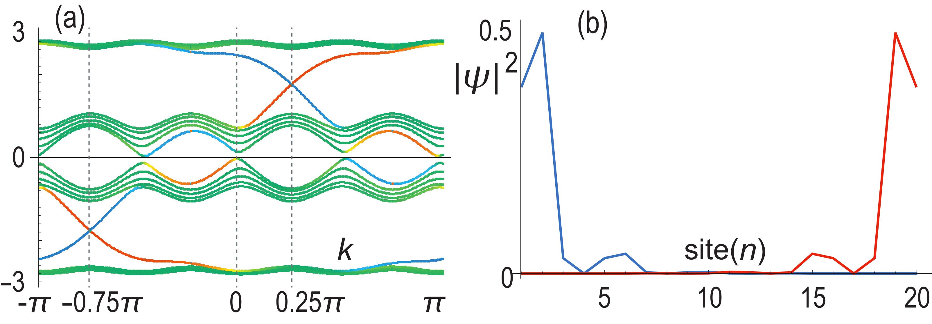
Figure 1: (a) Band structure of the matrix $\kappa M_{nm}$ in nanoribbon geometry. Curves in red (blue) indicate the left(right)-localized edge states, while those in green indicate the bulk states. The horizontal axis is the momentum $k$ ranging from $-\pi$ to $\pi$. The vertical axis is the energy in units of $\kappa$. (b) The LDOS $|\psi_{n}|^{2}$ at $k=0.25\pi$. It is found to be localized at the edges. The horizontal axis is the lattice site $n$. We have taken the width of the nanoribbon $L=20$.

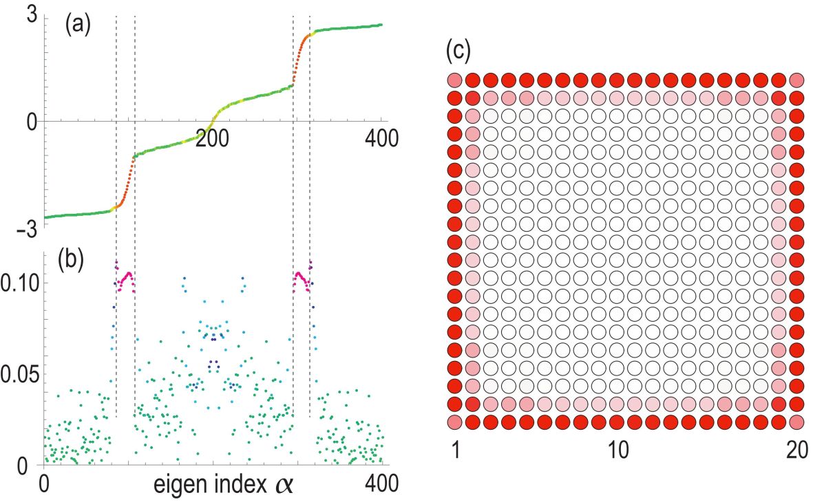
Figure 2: (a) Eigenspectrum of the matrix $\kappa M_{nm}$ in square geometry. The red parts of a curve indicate the edge states, while the green parts indicate the bulk states. The horizontal axis is the eigen index $\alpha$ of the state $\bar{\psi}_{n}^{\left(\alpha\right)}$. The vertical axis is the energy in units of $\kappa$. (b) The component $|c_{\alpha}|^{2}$ corresponding to the eigenenergy in (a). (c) The LDOS $|\psi_{n}|^{2}$ designated by the strength of red. It is found to be localized along the edges. We have used a square with size $20\times 20$.

Next, we calculate the eigenspectrum of the matrix $\kappa M$ in square geometry, which is shown in Fig.2(a). We also show the LDOS for an edge state in Fig.2(c), where the eigenfunction is well localized at the edge of the square.

Quench dynamics: We study a quench dynamics by giving a pulse to one site on the edge initially and by examining its time evolution. Namely, we solve the nonlinear Schrödinger equation (1) under the initial condition,

$$\psi_{0}\left(n_{x},n_{y}\right)=\delta\left(n_{x}-L_{x}/2,n_{y}-1\right),$$ (4)

where $L_{x}$ is the length of the edge along the $x$ axis, $L_{x}$ being an even number.

Scale transformation: By making a scale transformation

$$\psi_{j}=1/\sqrt{\xi}\psi_{j}^{\prime},$$ (5)

it follows from (1) that

$$i\frac{d\psi_{n}^{\prime}}{dt}+\kappa\sum_{m}M_{nm}\psi_{m}^{\prime}+\left|\psi_{n}^{\prime}\right|^{2}\psi_{n}^{\prime}=0,$$ (6)

where the nonlinearity parameter $\xi$ is removed.

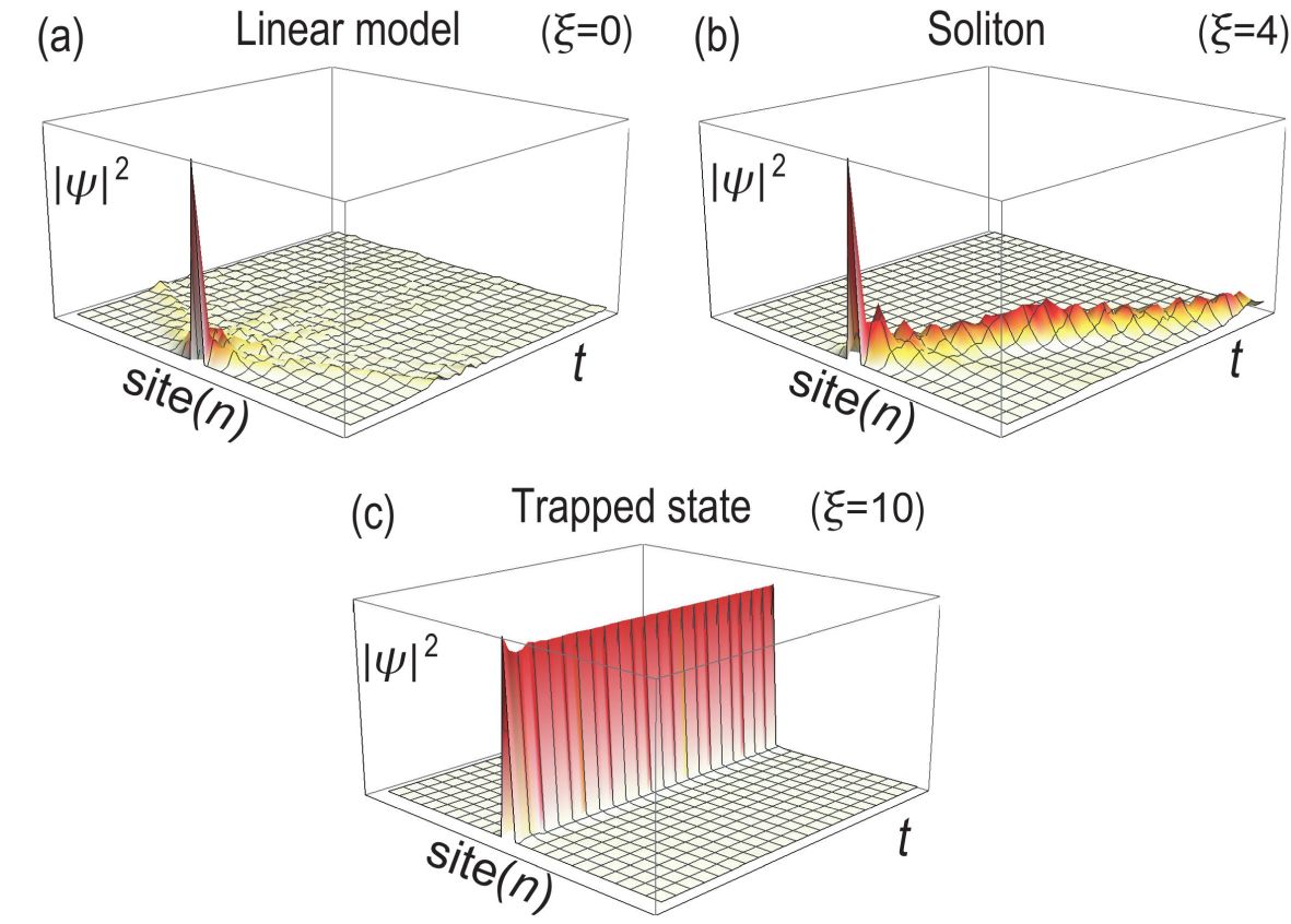
Figure 3: Time evolution of the LDOS $|\psi_{n}|^{2}$ (a) in the linear model with $\xi=0$, (b) in a nonlinear model with $\xi=4$ and (c) in a strong nonlinear model with $\xi=10$. We have used a square sample with size $20\times 20$.

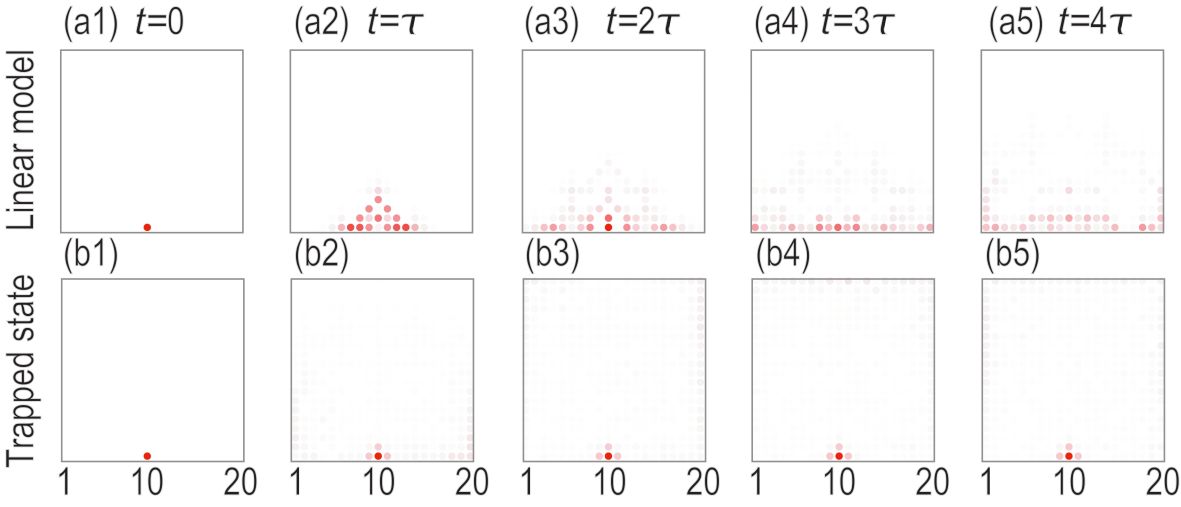
Figure 4: Time evolution of the spatial profile of the LDOS in a whole square sample with size $20\times 20$. (a1)$\sim$(a8) The LDOS in the linear model with $\xi=0$, where it diffuses as time passes. (b1)$\sim$(b8) The LDOS in a strong nonlinear model with $\xi=10$, where it is unchanged as time passes: The time step is $\tau=2$ in units of $1/\kappa$.

We are interested in the dynamics starting from a localized state at $\left(L_{x}/2,1\right)$ under the initial condition (4). This initial condition is transformed to

$$\psi_{0}^{\prime}\left(n_{x},n_{y}\right)=\sqrt{\xi}\delta\left(n_{x}-L_{x}/2,n_{y}-1\right).$$ (7)

Namely, the quench dynamics subject to Eq.(1) is reproduced with the use of the nonlinear equation (6) with the modified initial condition (7). Consequently, it is possible to use a single sample to investigate the quench dynamics at various nonlinearity only by changing the initial condition as in (7).

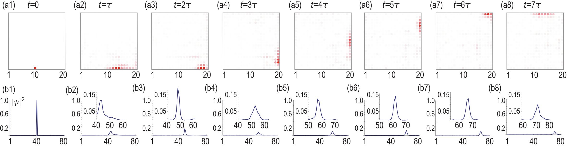
Figure 5: Time evolution of the LDOS $|\psi_{n}|^{2}$ in the nonlinear model with $\xi=4$. (a1)$\sim$(a8) Spatial profile of the LDOS in a whole square sample with size $20\times 20$. (b1)$\sim$(b8) The LDOS along the edge of a rectangular sample with size $80\times 10$. The time step is $\tau=10$ in units of $1/\kappa$. Each inset shows an enlarged figure of a soliton.

First, we study the linear model by setting $\xi=0$ in Eq.(1). We expand the initial state (4) by the eigenfunctions

$$\psi_{0}=\sum_{\alpha}c_{\alpha}\bar{\psi}_{n}^{\left(\alpha\right)},$$ (8)

where $\bar{\psi}_{n}^{\left(\alpha\right)}$ is the eigenfunction of the matrix $\kappa M_{nm}$ and $\alpha$ is the index of the eigenenergy,

$$\kappa M_{nm}\bar{\psi}_{m}^{\left(\alpha\right)}=E_{\alpha}\bar{\psi}_{n}^{\left(\alpha\right)}.$$ (9)

The square of the component $\left|c_{\alpha}\right|^{2}$ is shown in Fig.2(b). It has peaks at the edge states colored in red, but it has also values in the bulk states colored in green.

We show the time evolution of the amplitude $\left|\psi_{n}\right|^{2}$ along the edge in Fig.3, when a pulse is given to the site $\left(L_{x}/2,1\right)$ as an initial condition. It exhibits distinct behaviors depending on $\xi$. Typical behaviors are as follows. When $\xi=0$, the localized state rapidly spreads as in Fig.3(a). On the other hand, when $\xi=4$, we observe a soliton-like wave propagation as in Fig.3(b). When $\xi=10$, the state remains localized as in Fig.3(c). We explore these characteristic phenomena more in detail.

Linear model: The time evolution of the LDOS $\left|\psi_{n}\right|^{2}$ for the linear model ($\xi=0$) is shown in Fig.4(a1)$\sim$(a5). The amplitude spreads not only along the edge but also into the bulk in a symmetric way between the right and the left sides. One might expect a one-way propagation as in the Haldane model because the edge states are chiral. However, this is not the case in the present model, because there are two pairs of chiral edge states with opposite chiralities as shown in Fig.1(a). In fact, the occupation of these two opposite chiral edge states is identical as shown in Fig.2(b). Namely, there are equal numbers of the right-going and left-going propagating waves, which results in the symmetric spreading of the wave propagation. Another feature is that considerable amounts of the amplitude $\left|\psi_{n}\right|^{2}$ penetrate into the bulk although we start with the state localized at the edge as in Eq.(4). This is due to the fact that $\left|c_{\alpha}\right|^{2}$ is nonzero also for bulk states as we have already pointed out: See Fig.2(b).

Chiral edge soliton: We next study the nonlinear model with $\xi=4$, whose quench dynamics is shown in Fig.5(a1)$\sim$(a8) for a square with size $20\times 20$ and in Fig.5(b1)$\sim$(b8) for a rectangle with size $80\times 10$. There are two features absent in the linear model. One is that the wave packet propagates rightward. Namely, the wave packet dynamics becomes chiral due to the nonlinear term. A remarkable feature is that the shape of the wave packet remains almost unchanged after a certain time. It is the case even after the wave packet turns a corner, as shown in Fig.5(a4) and (a8). It looks like a solitary wave or a soliton. Hence, it may well be a chiral edge soliton. We may interpret that an initial pulse excites a chiral edge soliton and other modes, where all the other modes spread into the bulk and disappear.

A comment is in order for the presence of slight oscillations in the propagation of a solitonic wave. This is due to a lattice effect associated with the lack of the continuous translational symmetry. The form of a soliton slightly deforms depending on the mismatch between the center of the wave packet and lattice pointsMuk . This is in contrast to the continuum theory, where a soliton moves without deformation.

The mean position $\left\langle x\right\rangle$ of the wave packet is given by

$$\left\langle x\right\rangle\equiv\sum_{n_{x},n_{y}}\left(n_{x}-L_{x}/2\right)\left|\psi_{n_{x},n_{y}}\right|^{2}.$$ (10)

We calculate the time evolution of $\left\langle x\right\rangle$ for various $\xi$, fit the position by a linear function $\left\langle x\right\rangle=v_{x}t$, and estimate the velocity $v_{x}$ as a function of $\xi$, whose result is summarized in Fig.6(a). The velocity is zero for $\xi=0$. It linearly increases for $0<\xi\lesssim 4$, suddenly decreases for $\xi\gtrsim 4$, and makes a jump at $\xi\approx 5.6$.

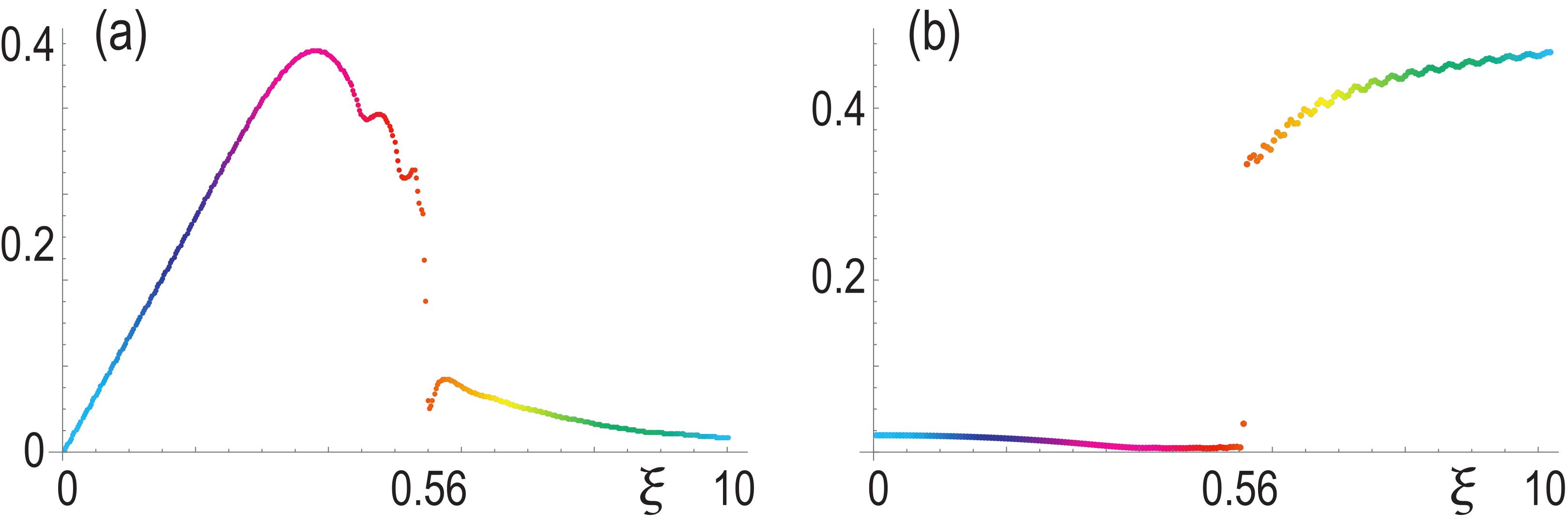
Figure 6: (a) Velocity $v_{x}$ as a function of $\xi$, which is linear for $\xi\lesssim 4$. The vertical axis is velocity in the unit $\kappa$, while the horizontal axis is $\xi$. (b) Amplitude $|\psi_{L_{x}/2,1}|^{2}$ at the initial point as a function of $\xi$. Color indicates the value of $\xi$. The horizontal axis is $\xi$. We have used a sample with the size $40\times 10$.

Self-trapped state: The jump indicates a self-trapping transition. We show the time evolution of the spatial distribution in a strong nonlinear model ($\xi=10$) in Fig.4(b1)$\sim$(b5), where the state remains localized. In order to show the self-trapping transition, we calculate the amplitude at the initial site after enough time,

$$\left|\psi_{0}\right|^{2}\equiv\lim_{t\rightarrow\infty}\left|\psi_{L_{x}/2,1}\left(t\right)\right|^{2}.$$ (11)

We show it as a function of $\xi$ in Fig.6(d). There is a sharp transition around $\xi\simeq 5.6$. The nonlinear-induced self-trapping transition has been discussed in other contextsCai ; NLPhoto ; NLSkin .

In the strong nonlinear regime ($\xi\gg 1$), we may approximate Eq.(1) as

$$i\frac{d\psi_{n}}{dt}=-\xi\left|\psi_{n}\right|^{2}\psi_{n},$$ (12)

where all equations are separated one another. The solution is $\psi_{n}\left(t\right)=r_{n}e^{i\theta_{n}\left(t\right)}$, with a constant $r_{n}$ and $\theta_{n}=\xi r_{n}^{2}t+c$. Hence, the amplitude does not decrease. By imposing the initial condition (4), we have $r_{n}=1$ for $t=0$. Namely, the state is strictly localized at the initial site as in Fig.3(c).

Discussion: We have studied nonlinear effects on the chiral edge state in the nonlinear Schrödinger equation. We have revealed characteristic features depending on the magnitude of the nonlinearity. When the nonlinearity is negligible, an initial pulse spreads symmetrically and diffuses. When it is intermediate, a chiral edge soliton is formed from an initial pulse. When it is strong enough, the self-trapping state appears.

The nonlinear term is an interaction term, which is diagonal in the real space. On the other hand, the hopping matrix $M$ is diagonal in the momentum space as in Eq.(3). Hence, there is a competition between the real-space and momentum-space diagonalizations in the nonlinear Schrödinger equation. In the linear model, the momentum is a good number, where the plane wave is an eigenstate. On the other hand, in the strong nonlinear model, the real space is a good number, where the self-trapping state is an eigenstate. A chiral soliton emerges between these two limits.

It will be possible to observe these phenomena experimentally in various nonlinear topological systems. The photonic system is a good candidate, where the nonlinear term is generated as the Kerr term, and the topological edge states must be directly observed by photoluminescence. It is also possible to observe the time evolution of the edge statesHafezi ; Bandres . Furthermore, the nonlinearity is controlled only by changing the intensity of light without changing a sample.

The author is very much grateful to N. Nagaosa for helpful discussions on the subject. This work is supported by the Grants-in-Aid for Scientific Research from MEXT KAKENHI (Grants No. JP17K05490 and No. JP18H03676). This work is also supported by CREST, JST (JPMJCR16F1 and JPMJCR20T2).

References

- (1) S. Raghu and F. D.M. Haldane, Phys. Rev. A 78, 033834 (2008)
- (2) M. Hafezi, E. Demler, M. Lukin, J. Taylor, Nature Physics 7, 907 (2011).
- (3) M. Hafezi, S. Mittal, J. Fan, A. Migdall, J. Taylor, Nature Photonics 7, 1001 (2013).
- (4) A. B. Khanikaev, S. H. Mousavi, W.-K. Tse, M. Kargarian, A. H. MacDonald, G. Shvets, Nature Materials 12, 233 (2013).
- (5) L.H. Wu and X. Hu, Phys. Rev. Lett. 114, 223901 (2015).
- (6) L. Lu. J. D. Joannopoulos and M. Soljacic, Nature Photonics 8, 821 (2014).
- (7) T. Ozawa, H. M. Price, N. Goldman, O. Zilberberg and I. Carusotto Phys. Rev. A 93, 043827 (2016).
- (8) D. Leykam and Y. D. Chong, Phys. Rev. Lett. 117, 143901 (2016).
- (9) A. B. Khanikaev and G. Shvets, Nature Photonics 11, 763 (2017).
- (10) X. Zhou, Y. Wang, D. Leykam and Y. D. Chong, New J. Phys. 19, 095002 (2017).
- (11) P. St-Jean, V. Goblot, E. Galopin, A. Lemaitre, T. Ozawa, L. Le Gratiet, I. Sagnes, J. Bloch and A. Amo, Nature Photonics 11, 651 (2017).
- (12) Y. Ota, R. Katsumi, K. Watanabe, S. Iwamoto and Y. Arakawa, Communications Physics 1, 86 (2018)
- (13) T. Ozawa, H. M. Price, A. Amo, N. Goldman, M. Hafezi, L. Lu, M. C. Rechtsman, D. Schuster, J. Simon, O. Zilberberg and L. Carusotto, Rev. Mod. Phys. 91, 015006 (2019).
- (14) Y. Ota, F. Liu, R. Katsumi, K. Watanabe, K. Wakabayashi, Y. Arakawa and S. Iwamoto, Optica 6, 786 (2019).
- (15) T. Ozawa and H. M. Price, Nature Reviews Physics 1, 349 (2019).
- (16) A. E. Hassan, F. K. Kunst, A. Moritz, G. Andler, E. J. Bergholtz, M. Bourennane, Nature Photonics 13, 697 (2019).
- (17) Y. Ota, K. Takata, T. Ozawa, A. Amo, Z. Jia, B. Kante, M. Notomi, Y. Arakawa, S.i Iwamoto, Nanophotonics 9, 547 (2020).
- (18) M. Li, D. Zhirihin, D. Filonov, X. Ni, A. Slobozhanyuk, A. Alu and A. B. Khanikaev, Nature Photonics 14, 89 (2020).
- (19) H. Yoshimi, T. Yamaguchi, Y. Ota, Y. Arakawa and S. Iwamoto, Optics Letters 45, 2648 (2020).
- (20) M. Kim, Z. Jacob and J. Rho, Light: Science and Applications 9, 130 (2020).
- (21) S. Iwamoto, Y. Ota and Y. Arakawa, Optical Materials Express 11, 319 (2021).
- (22) E. Prodan and C. Prodan, Phys. Rev. Lett. 103, 248101 (2009).
- (23) Z. Yang, F. Gao, X. Shi, X. Lin, Z. Gao, Y. Chong and B. Zhang, Phys. Rev. Lett. 114, 114301 (2015).
- (24) P. Wang, L. Lu and K. Bertoldi, Phys. Rev. Lett. 115, 104302 (2015).
- (25) M. Xiao, G. Ma, Z. Yang, P. Sheng, Z. Q. Zhang and C. T. Chan, Nat. Phys. 11, 240 (2015).
- (26) C. He, X. Ni, H. Ge, X.-C. Sun,Y.-B. Chen1 M.-H. Lu, X.-P. Liu, L. Feng and Y.-F. Chen, Nature Physics 12, 1124 (2016).
- (27) H. Abbaszadeh, A. Souslov, J. Paulose, H. Schomerus and V. Vitelli, Phys. Rev. Lett. 119, 195502 (2017).
- (28) H. Xue, Y. Yang, F. Gao, Y. Chong and B.Zhang, Nature Materials 18, 108 (2019).
- (29) X. Ni, M. Weiner, A. Alu and A. B. Khanikaev, Nature Materials 18, 113 (2019).
- (30) M. Weiner, X. Ni, M. Li, A. Alu, A. B. Khanikaev, Science Advances 6, eaay4166 (2020).
- (31) H. Xue, Y. Yang, G. Liu, F. Gao, Y. Chong and B. Zhang, Phys. Rev. Lett. 122, 244301 (2019).
- (32) C. L. Kane and T. C. Lubensky, Nature Phys. 10, 39 (2014).
- (33) B. Gin-ge Chen, N. Upadhyaya and V. Vitelli, PNAS 111, 13004 (2014).
- (34) L. M. Nash, D. Kleckner, A. Read, V. Vitelli, A. M. Turner and W. T. M. Irvine, PNAS 112, 14495 (2015).
- (35) J. Paulose, A. S. Meeussen and V. Vitelli, PNAS 112, 7639 (2015).
- (36) R. Susstrunk, S. D. Huber, Science 349, 47 (2015).
- (37) S. Imhof, C. Berger, F. Bayer, J. Brehm, L. Molenkamp, T. Kiessling, F. Schindler, C. H. Lee, M. Greiter, T. Neupert, R. Thomale, Nat. Phys. 14, 925 (2018).
- (38) C. H. Lee , S. Imhof, C. Berger, F. Bayer, J. Brehm, L. W. Molenkamp, T. Kiessling and R. Thomale, Communications Physics, 1, 39 (2018).
- (39) T. Helbig, T. Hofmann, C. H. Lee, R. Thomale, S. Imhof, L. W. Molenkamp and T. Kiessling, Phys. Rev. B 99, 161114 (2019).
- (40) Y. Lu, N. Jia, L. Su, C. Owens, G. Juzeliunas, D. I. Schuster and J. Simon, Phys. Rev. B 99, 020302 (2019).
- (41) Y. Li, Y. Sun, W. Zhu, Z. Guo, J. Jiang, T. Kariyado, H. Chen and X. Hu, Nat. Com. 9, 4598 (2018).
- (42) M. Ezawa, Phys. Rev. B 98, 201402(R) (2018).
- (43) M. Ezawa, Phys. Rev. B 99, 201411(R) (2019).
- (44) M. Ezawa, Phys. Rev. B 99, 121411(R) (2019).
- (45) N. Malkova, I. Hromada, X. Wang, G. Bryant and Z. Chen, Opt. Lett. 34, 1633 (2009).
- (46) M. Xiao, Z. Q. Zhang and C. T. Chan, Phys. Rev. X 4, 021017 (2014).
- (47) M. Parto, S. Wittek, H. Hodaei, G. Harari, M. A. Bandres, J. Ren, M. C. Rechtsman, M. Segev, D. N Christodoulides and M. Khajavikhan, Phys. Rev. Lett. 120 (11), 113901 (2018).
- (48) Lukas J. Maczewsky, Matthias Heinrich, Mark Kremer, Sergey K. Ivanov, Max Ehrhardt, Franklin Martinez, Yaroslav V. Kartashov, Vladimir V. Konotop, Lluis Torner, Dieter Bauer, Alexander Szameit, Science 370, 701 (2010).
- (49) D. Smirnova, D. Leykam, Y. Chong and Y. Kivshar, Applied Physics Reviews 7, 021306 (2020).
- (50) T. Tuloup, R. W. Bomantara, C. H. Lee and J. Gong, Phys. Rev. B 102, 115411 (2020).
- (51) S. Kruk, A. Poddubny, D. Smirnova, L. Wang, A. Slobozhanyuk, A. Shorokhov, I. Kravchenko, B. Luther-Davies and Y. Kivshar, Nature Nanotechnology 14, 126 (2019).
- (52) M. Ezawa, Phys. Rev. B 104, 235420 (2021).
- (53) M. S. Kirsch, Y. Zhang, M. Kremer, L. J. Maczewsky, S. K. Ivanov, Y. V. Kartashov, L. Torner, D. Bauer, A. Szameit and M. Heinrich, Nature Physics 17, 995 (2021).
- (54) M. Ezawa, arXiv:2111.10707
- (55) D. D. J. M. Snee, Y.-P. Ma, Extreme Mechanics Letters 100487 (2019).
- (56) P.-W. Lo, K. Roychowdhury, B. G.-g. Chen, C. D. Santangelo, C.-M. Jian, M. J. Lawler, Phys. Rev. Lett. 127, 076802 (2021).
- (57) M. Ezawa, J. Phys. Soc. Jpn. 90, 114605 (2021).
- (58) M. Ezawa, arXiv:2110.15602
- (59) Y. Hadad, J. C. Soric, A. B. Khanikaev, and A. Alù, Nature Electronics 1, 178 (2018).
- (60) K. Sone, Y. Ashida, T. Sagawa, arXiv:2012.09479.
- (61) M. Ezawa, arXiv:2105.10851.
- (62) F. Zangeneh-Nejad and R. Fleury, Phys. Rev. Lett. 123, 053902 (2019).
- (63) D. N. Christodoulides, F. Lederer and Y. Silberberg, Nature 424, 817 (2003)
- (64) A. Szameit, D. Blöer, J. Burghoff, T. Schreiber, T. Pertsch, S. Nolte, A. Tünnermann and F. Lederer, Optics Express 13, 10552 (2005).
- (65) M. A. Gorlach, A. P. Slobozhanyuk, Nanosystems: Physics, Cheminstry, Mathematics, 8, 695 (2017).
- (66) D. A. Dobrykh, A. V. Yulin, A. P. Slobozhanyuk, A. N. Poddubny and Y. S. Kivshar Phys. Rev. Lett. 121, 163901 (2018)
- (67) S. Mukherjee and M. C. Rechtsman, Phys. Rev. X 11, 041057 (2021)
- (68) Z. Zhang, R. Wang, Y. Zhang, Y. V. Kartashov, F. Li, H. Zhong, H. Guan, K. Gao, F. Li, Y. Zhang and M. Xiao, Nat. Com. 11, 1902 (2020).
- (69) M. Ezawa, arXiv:2112.06241.
- (70) J. C. Eilbeck, P. S. Lomdahl and A. C. Scott, Physica D 16, 318, (1985).
- (71) P. G. Kevrekidis, K. O. Rasmussen and A. R. Bishop, Int. J. Mod. Phys. B 15, 2833 (2001).
- (72) M. A. Bandres, S. Wittek, G. Harari, M. Parto, J. Ren, Mordechai Segev, Demetrios N. Christodoulides, Mercedeh Khajavikhan Science 359, 1231 (2018).
- (73) G. Harari, M. A. Bandres, Y. Lumer, M. C. Rechtsman, Y. D. Chong, M. Khajavikhan, D. N. Christodoulides, M. Segev, Science 359, eaar4003 (2018).
- (74) D. Cai, A. R. Bishop and N. Gronbech-Jensen, Phys. Rev. Lett. 72, 591 (1994).