Exponential family measurement error models for single-cell CRISPR screens
Abstract
CRISPR genome engineering and single-cell RNA sequencing have transformed biological discovery. Single-cell CRISPR screens unite these two technologies, linking genetic perturbations in individual cells to changes in gene expression and illuminating regulatory networks underlying diseases. Despite their promise, single-cell CRISPR screens present substantial statistical challenges. We demonstrate through theoretical and real data analyses that a standard method for estimation and inference in single-cell CRISPR screens –“thresholded regression” – exhibits attenuation bias and a bias-variance tradeoff as a function of an intrinsic, challenging-to-select tuning parameter. To overcome these difficulties, we introduce GLM-EIV (“GLM-based errors-in-variables”), a new method for single-cell CRISPR screen analysis. GLM-EIV extends the classical errors-in-variables model to responses and noisy predictors that are exponential family-distributed and potentially impacted by the same set of confounding variables. We develop a computational infrastructure to deploy GLM-EIV across hundreds of processors on clouds (e.g., Microsoft Azure) and high-performance clusters. Leveraging this infrastructure, we apply GLM-EIV to analyze two recent, large-scale, single-cell CRISPR screen datasets, yielding several novel insights.Cloud computing, genome engineering, GLM, GWAS, latent variable model
1 Introduction
CRISPR is a genome engineering tool that has enabled scientists to precisely edit human and nonhuman genomes, opening the door to new medical therapies (Musunuru and others, 2021) and transforming biological discovery (Przybyla and Gilbert, 2021). Recently, scientists have paired CRISPR genome engineering with single-cell RNA sequencing (Datlinger and others, 2017). The resulting assays, known as“single-cell CRISPR screens,” link genetic perturbations in individual cells to changes in gene expression, enabling scientists to causally map genome wide association study (GWAS) variants to their target genes at genome-wide scale (Morris and others, 2023).
Despite their promise, single-cell CRISPR screens present substantial statistical challenges. A major difficulty is that the “treatment” — i.e., the presence or absence of a CRISPR perturbation — is assigned randomly to cells and is not directly observable. As a consequence, one cannot know with certainty which cells were perturbed. Instead, one must leverage an indirect, quantitative proxy of perturbation presence or absence to “guess” which cells received a perturbation. This indirect proxy takes the form of a so-called guide RNA count, with higher counts indicating that a cell is more likely to have been perturbed. A standard approach to single-cell CRISPR screen analysis is to impute perturbation assignments onto the cells by simply thresholding the guide RNA counts; using these imputations, one can attempt to estimate the effect of the perturbation on gene expression. We call this standard approach “thresholded regression” or the “thresholding method.”
We study estimation and inference in single-cell CRISPR screens from a statistical perspective, formulating the data generating mechanism using a new class of measurement error models. We assume that the response variable is a GLM of an underlying predictor variable and vector of confounders . We do not observe directly; rather, we observe a noisy version of that itself is a GLM of and the same set of confounders . The goal of the analysis is to estimate the effect of on using the observed data only. In the context of the biological application, , , , and are CRISPR perturbations, guide RNA counts, gene expressions, and technical confounders, respectively.
Our work makes two main contributions. First, we conduct a detailed study of the thresholding method. Notably, we demonstrate on real data that the thresholding method exhibits attenuation bias and a bias-variance tradeoff as a function of the selected threshold, and we recover these phenomena in precise mathematical terms in a simplified Gaussian setting. Second, we introduce a new method, GLM-EIV (“GLM-based errors-in-variables”), for single-cell CRISPR screen analysis. GLM-EIV extends the classical errors-in-variables model (Carroll and others, 2006) to responses and noisy predictors that are exponential family-distributed and potentially impacted by the same set of confounding variables. GLM-EIV thereby implicitly estimates the probability that each cell was perturbed, obviating the need to explicitly impute perturbation assignments via thresholding. We implement several statistical accelerations to bring the cost of GLM-EIV down to within about an order of magnitude of the thresholding method. We additionally develop a Docker-containerized application to deploy GLM-EIV at-scale across tens or hundreds of processors on clouds (e.g., Microsoft Azure) and high-performance clusters.
We find that single-cell CRISPR screens can be roughly categorized into two problem settings: the more challenging “high background contamination” setting and the less challenging “low background contamination” setting. GLM-EIV outperforms thresholded regression by a considerable margin in the high background contamination setting; in the low background contamination setting, by contrast, GLM-EIV and thresholded regression perform similarly, provided that the optimal threshold is selected for use in the thresholded regression model. We show that a simplified version of the GLM-EIV model can be used to identify this optimal threshold in the low background contamination setting, thereby neutralizing a tuning parameter that until this point has been challenging to select. Thus, we conclude that, across problem settings, GLM-EIV serves as a useful tool in the single-cell CRISPR screen analysis toolkit.
2 Assay background
There are several classes of single-cell CRISPR screen assays, each suited to answer a different set of biological questions. In this work we mainly focus on high-multiplicity of infection (MOI) single-cell CRISPR screens, which we motivate and describe here. The human genome consists of genes, enhancers (segments of DNA that regulate the expression of one or more genes), and other genomic elements (that are not of relevance to the current work). GWAS have revealed that the majority () of variants associated with diseases lie outside genes and inside enhancers (Gallagher and Chen-Plotkin, 2018). These noncoding variants are thought to contribute to disease by modulating the expression of one or more disease-relevant genes. Scientists do not know the gene (or genes) through which most noncoding variants exert their effect, limiting the interpretability of GWAS results. A central open challenge in genetics, therefore, is to link enhancers that harbor GWAS variants to the genes that they target at genome-wide scale (Morris and others, 2023).
High MOI single-cell CRISPR screens are among the most promising biotechnologies for solving this challenge. High MOI single-cell CRISPR screens combine CRISPR interference (CRISPRi) — a version of CRISPR that represses a targeted region of the genome — with single-cell sequencing. The experimental protocol is as follows. First, the scientist develops a library of several hundred to several thousand CRISPRi perturbations, each designed to target a candidate enhancer for repression. The scientist then cultures tens or hundreds of thousands of cells and delivers the CRISPRi perturbations to these cells. The perturbations assort into the cells randomly, with each cell receiving on average 10-40 distinct perturbations. Conversely, a given perturbation enters about 0.1-2% of cells (this work).
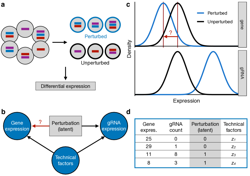
After waiting several days for CRISPRi to take effect, the scientist profiles each cell’s transcriptome (i.e., its gene expressions) and the set of perturbations that it received. Finally, the scientist conducts perturbation-to-gene association analyses. Figure 1a depicts this process schematically, with colored bars (blue, red, and purple) representing distinct perturbations. For a given perturbation (e.g., the perturbation represented in blue), the scientist partitions the cells into two groups: those that received the perturbation (top) and those that did not (bottom). Next, for a given gene, the scientist runs a differential expression analysis across the two groups of cells, producing an estimate for the magnitude of the gene expression change in response to the perturbation. If the estimated change in expression is large, the scientist can conclude that the enhancer targeted by the perturbation exerts a strong regulatory effect on the gene. This procedure is repeated for a large set of preselected perturbation-gene pairs. The enhancer-by-enhancer approach is valid because the perturbations assort into cells approximately independently of one another.
The genomics literature has produced a few applied methods for single-cell CRISPR screen analysis (Gasperini and others, 2019; Xie and others, 2019; Barry and others, 2021). Gasperini et al. applied negative binomial GLMs (as implemented in the Monocle software; Trapnell and others (2014)) to carry out the differential expression analysis described above. Xie et al., by contrast, applied chi-squared-like tests of independence for this purpose. Both of these approaches have limitations: the former is not robust to misspecification of the gene expression model, and the latter is unable to correct for the presence of technical confounders. Recently, Barry et al. introduced SCEPTRE, a custom implementation of the conditional randomization test (Candès and others, 2018; Liu and others, 2021) tailored to single-cell CRISPR screen data. SCEPTRE simultaneously adjusts for confounder presence and ensures robustness to expression model misspecification, overcoming limitations of the prior methods and demonstrating state-of-the-art sensitivity and specificity on single-cell CRISPR screen data. In this work we tackle a set of analysis challenges that are complimentary to those addressed by SCEPTRE. Most importantly, we seek to account for the fact that the perturbation is measured with noise, an issue that all available methods (including SCEPTRE) assume away via thresholding. Additionally, we seek to estimate (with confidence) the effect size of a perturbation on gene expression change, an objective that is challenging to attain within the nonparametric hypothesis testing framework of SCEPTRE.
3 Analysis challenges and proposed statistical model
High MOI single-cell CRISPR screens present several statistical challenges, four of which we highlight here. Throughout, we consider a single perturbation-gene pair. First, the “treatment” variable — i.e., the presence or absence of a perturbation — cannot be directly observed. Instead, perturbed cells transcribe molecules called guide RNAs (or gRNAs) that serve as indirect proxies of perturbation presence. We must leverage these gRNAs to impute (explicitly or implicitly) perturbation assignments onto the cells (Figure 1b). Second, “technical factors” — sources of variation that are experimental rather than biological in origin — impact the measurement of both gene and gRNA expressions and therefore act as confounders (Figure 1b). Third, the gene and gRNA data are sparse, discrete counts. Consequently, classical statistical approaches that assume Gaussianity or homoscedasticity are inapplicable. Finally, sequenced gRNAs sometimes map to cells that have not received a perturbation. This phenomenon, which we call “background contamination,” results from errors in the sequencing and alignment processes. The marginal distribution of the gRNA counts is best conceptualized as a mixture model (Figure 1c; Gaussian distributions used for illustration purposes only). Unperturbed and perturbed cells both exhibit nonzero gRNA count distributions, but this distribution is shifted upward for perturbed cells. Figure 1d shows example data on four (of possibly tens or hundreds of thousands of) cells. The analysis objective is to leverage the gene expressions and gRNA counts to estimate the effect of the (latent) perturbation on gene expression, accounting for the technical factors.
We propose to model the single-cell CRISPR screen data-generating process using a pair of GLMs. Let be the number of cells assayed in the experiment. Consider a single perturbation and a single gene. For cell , let indicate perturbation presence or absence; let be the number of gene transcripts sequenced; let be the number of gRNA transcripts sequenced; let be the number of gene transcripts sequenced across all genes (i.e., the library size or sequencing depth); let be the gRNA library size; and finally, let be the cell-specific covariates, including sequencing batch, percent mitochondrial reads, etc. (We note that most single-cell CRISPR screens have been carried out on cell lines consisting of a uniform cell type; however, if multiple cell types are present in the data, then cell type could be included as a covariate.) The letters “m,” “g”, and “d” stand for “mRNA,” “gRNA,” and “depth,” respectively.
Building on the work of several previous authors (Townes and others, 2019; Hafemeister and Satija, 2019), Sarkar and Stephens (2021) proposed a simple strategy for modeling single-cell gene expression data, which, in the framework of negative binomial GLMs, is equivalent to using the log-transformed library size as an offset term. Sarkar and Stephens’ framework enjoys strong theoretical and empirical support; therefore, we generalize their approach to model both gene and gRNA modalities in single-cell CRISPR screen experiments. To this end we assume that the gene expression counts are given by
| (1) |
where (i) is a negative binomial distribution with mean and known size parameter ; (ii) and are unknown parameters; and (iii) is an offset term. (We note that the “size parameter” is simply the inverse of the negative binomial dispersion parameter; “size parameter” does not refer to library size in this context.) Similarly, we model the gRNA counts by
| (2) |
where , , , , , and are analogous. We use a negative binomial GLM to model the gRNA counts as well as the gene expressions because the gRNA transcripts are generated via the same biological mechanism as the gene transcripts (Datlinger and others, 2017; Hill and others, 2018). We model the marginal perturbation as , where is an unobserved binary variable indicating presence () or absence () of the perturbation. We restrict , the probability of perturbation, to the interval to ensure that the model is identifiable; this restriction is quite reasonable given that each perturbation infects only a small fraction of cells. The gRNA intercept term controls the ambient level of gRNA expression, i.e. the rate at which gRNA reads are generated in the absence of the perturbation. The perturbation coefficient controls the extent to which perturbed and unperturbed cells differentially express the gRNA; the target of inference is challenging to estimate when is close to zero, as the gRNA distributions of the perturbed and unperturbed cells are hard to differentiate in this region of the problem space. Together, (1), (2), and the marginal distribution of define the negative binomial GLM-EIV model.
The log-transformed sequencing depth is included as an offset term in (1) so that can be interpreted as a relative expression. Exponentiating both sides of (1) reveals that the mean gene expression of the th cell is Because is the sequencing depth, is the fraction of all transcripts sequenced in the cell produced by the gene under consideration. The target of inference is the log fold change in expression in response to the perturbation, controlling for the technical factors. Fold change in this context is the ratio of the mean gene expression in perturbed cells to the mean gene expression in unperturbed cells. Hence, (i.e., ) indicates no change in expression, whereas (i.e., ) and (i.e., ) indicate an increase and decrease in expression, respectively.
In this work we analyzed two large-scale, high MOI, single-cell CRISPR screen datasets published by Gasperini and others (2019) and Xie and others (2019). Gasperini (resp., Xie) targeted approximately 6,000 (resp., 500) candidate enhancers in a population of approximately 200,000 (resp., 100,000) cells. Gasperini additionally designed several hundred positive control, gene-targeting perturbations and 50 non-targeting, negative control perturbations to assess method sensitivity and specificity.
4 Analysis of the thresholding method
We studied thresholding from empirical and theoretical perspectives, highlighting several potential limitations of the approach. In the context of the negative bionomial GLM-EIV model introduced above (1-2), the thresholding method leverages the gRNA counts (2) to impute the latent perturbation indicator (2), thereby reducing the full data generating process to a single, gene expression model (1). We studied Gasperini et al.’s variant of the thresholding method (i.e., thresholded negative binomial regression), as this version of the thresholding method is standard and relates most closely to GLM-EIV. The method is defined as follows:
-
1.
For a given threshold , let the imputed perturbation assignment be given by if and otherwise.
- 2.
-
3.
Fit a GLM to (3) to obtain an estimate and CI for the target of inference .
To shed light on empirical challenges of the thresholding method, we applied thresholded negative binomial regression to analyze the set of positive control perturbation-gene pairs in the Gasperini dataset. The positive control pairs consisted of perturbations that targeted gene transcription start sites (TSSs) for inhibition. Repressing the TSS of a given gene decreases its expression; therefore, the positive control pairs a priori are expected to exhibit a strong decrease in expression.
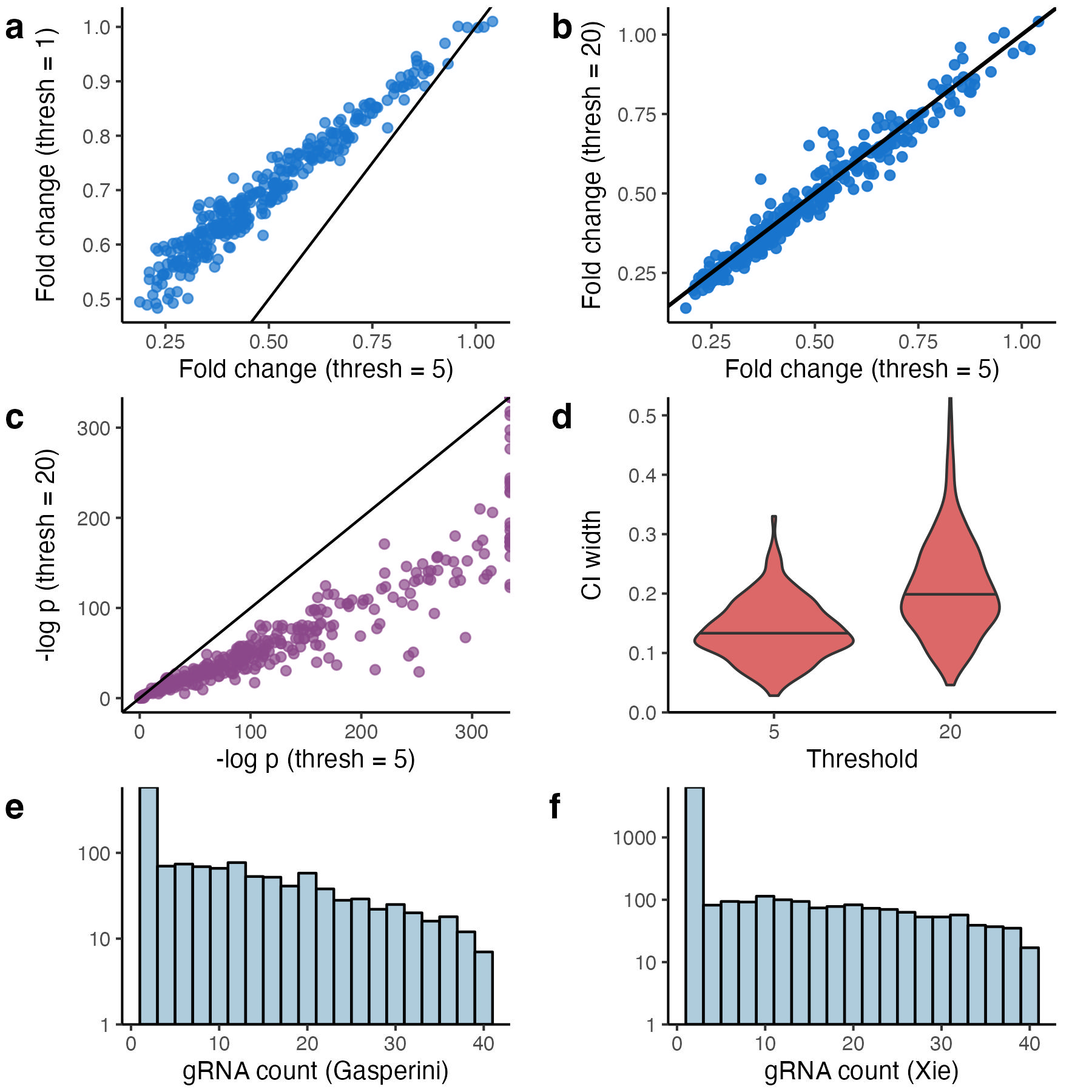
To investigate the sensitivity of the thresholding method to threshold choice, we deployed the method using three different choices for the threshold: 1, 5, and 20. We found that the chosen threshold substantially impacted the results (Figure 2a-b): estimates for fold change produced by threshold = 1 were smaller in magnitude (i.e., closer to the baseline of ) than those produced by threshold = 5. (Figure 2a.) On the other hand, estimates produced by threshold = 5 and threshold = 20 were more concordant (Figure 2b).
We reasoned that thresholded regression systematically underestimated true effect sizes on the positive control pairs, especially for threshold = 1. For a given perturbation, the majority () of cells are unperturbed. This imbalance leads to an asymmetry: misclassifying unperturbed cells as perturbed is intuitively “worse” than misclassifying perturbed cells as unperturbed. Misclassified unperturbed cells contaminate the set of truly perturbed cells, leading to attenuation bias; by contrast, misclassified perturbed cells are swamped in number and “neutralized” by the truly unperturbed cells. Setting the threshold to a large number reduces the unperturbed-to-perturbed misclassification rate, decreasing bias.
We hypothesized, however, that the reduction in bias obtained by selecting a large threshold causes the variance of the estimator to increase. To investigate, we compared -values and confidence intervals produced by threshold = 5 and threshold = 20 for the target of inference . We found that threshold = 5 yielded smaller (i.e., more significant) -values and narrower confidence intervals than did threshold = 20 (Figures 2c-d). We concluded that the threshold controls a bias-variance tradeoff: as the threshold increases, the bias of the estimator decreases and the variance increases.
Finally, to determine whether there is an “obvious” location at which to draw the threshold, we examined the empirical gRNA count distributions and checked for bimodality. Figures 2e and 2f display the empirical distribution of a randomly-selected gRNA from the Gasperini and Xie datasets, respectively (counts of omitted). The distributions peak at and then taper off gradually; there does not exist a sharp boundary that cleanly separates the perturbed from the unperturbed cells. Overall, we concluded that the thresholding method faces several challenges: (i) the threshold is a tuning parameter that significantly impacts the results; (ii) the threshold mediates an intrinsic bias-variance tradeoff; and (iii) the gRNA count distributions do not imply a clear threshold selection strategy.
Next, we studied the thresholding method from a theoretical perspective, recovering in a simplified Gaussian setting phenomena revealed in the empirical analysis. Due to space constraints we relegate this analysis to Appendix A, but we briefly summarize the main results here. First, we derived an exact expression for the asymptotic relative bias of the thresholding estimator Leveraging this exact expression, we showed that (i) the thresholding estimator strictly underestimates (in absolute value) the true value of over all choices of the threshold and over all values of the regression coefficients (an example of attenuation bias; Stefanski (2000)); and (ii) the magnitude of the bias decreases monotonically in , comporting with the intuition that the problem becomes easier as the gRNA mixture distribution becomes increasingly well-separated. Second, we derived an asymptotically exact bias-variance decomposition for , demonstrating that as the threshold tends to infinity, the bias decreases and the variance increases.
5 GLM-based errors-in-variables (GLM-EIV)
We introduce the general GLM-EIV model, which generalizes the negative binomial GLM-EIV model (1-2) to arbitrary exponential family response distributions and link functions, thereby providing much greater modeling flexibility. We derive efficient methods for estimation and inference in this model and develop a pipeline to deploy the model at-scale.
5.1 Model and model properties
The general GLM-EIV model uses an arbirary GLM to model the gene and gRNA modalities:
| (4) |
| (5) |
Here, (resp., ) is an exponential family distribution with mean (resp., ); and are the link function for the gene and gRNA models, respectively; and and are the (possibly zero) offset terms for the gene and gRNA models. In practice we typically set and to the log-transformed library sizes (i.e., and ). Again, we assume that the unobserved perturbation indicator is drawn from a distribution. More model details are available in Appendix B. A zero-inflated version of the GLM-EIV model is developed in Appendix C.
The GLM-EIV model can be seen as a generalization of the simple errors-in-variables model (when the predictor is binary); the latter is defined as follows:
| (6) |
where, and ,, and are independent. GLM-EIV extends (6) in at least three directions: first, GLM-EIV allows and to follow exponential family (i.e, not just Gaussian) distributions; second, GLM-EIV allows and to be related to through arbitrary (i.e., not just linear) link functions; and finally, GLM-EIV allows confounders to impact both and . Therefore, and can be conditionally dependent given , enabling GLM-EIV to capture more complex dependence relationships between and than is possible in (6) or other standard measurement error models.
5.2 Estimation and inference, and computational infrastructure
We derived an EM algorithm (Algorithm 1) to estimate the parameters of the GLM-EIV model. We briefly introduce some notation. Let be the vector of unknown gene model parameters and the vector of unknown gRNA model parameters. Let , , , and be the vector of gene expressions, gRNA expressions, gene library sizes, and gRNA library sizes. Finally, let be the observed design matrix; let be the augmented design matrix that results from concatenating the column of (unobserved) s to ; and let (resp, ) be the matrix that results from setting all of the s in to (resp., ).
The E step entails computing the membership probability (i.e., the probability of perturbation) in each cell. The membership probability of cell given the current parameter estimates and observed data is We can calculate this quantity by applying (i) Bayes rule, (ii) the conditional independence property of and , (iii) the density of and , and (iv) a log-sum-exp-type trick to ensure numerical stability. Next, we produce updated estimates , , and of the parameters by maximizing the M step objective function. It turns out that maximizing this objective function is equivalent to setting to the mean of the current membership probabilities and setting and to the fitted coefficients of a GLM weighted by the current membership probabilities (Algorithm 1). We iterate through the E and M steps until the log likelihood (43) converges (Appendix B). Our EM algorithm is reminiscent of (but distinct from) that of Ibrahim (1990), who also applied weighted GLM solvers to carry out an M step of an EM algorithm.
| Fit a GLM with responses , offsets , weights , design matrix , distribution , and link function . |
After fitting the model, we perform inference on the estimated parameters. The easiest approach, given the complexity of the log likelihood, would be to run a bootstrap. This strategy, however, is prohibitively slow, as the data are large and the EM algorithm is iterative. Therefore, we derived an analytic formula for the asymptotic observed information matrix using Louis’s Theorem (Louis (1982); Appendix B). Leveraging this analytic formula, we can calculate standard errors quickly, enabling us to perform inference in practice on real, large-scale data.
A downside of the the EM algorithm (Algorithm 1) is that it requires fitting many GLMs. Assuming that we run the algorithm 15 times using randomly-generated pilot estimates (to improve chances of convergence to the global maximum), and assuming that the algorithm iterates through E and M steps about 10 times per run, we must fit approximately 300 GLMs. (These numbers are based on exploratory applications of the method to real and simulated data.) We instead devised a strategy to produce a highly accurate pilot estimate of the true parameters, enabling us to run the algorithm once and converge upon the MLE within a few iterations. The strategy involves layering several statistical “tricks” on top of one another. Briefly, we first obtain pilot estimates for the nuisance parameters and by regressing the gene and gRNA expression vectors onto the observed design matrix ; the resulting estimates are close to the full GLM-EIV model maximum likelihood estimates because the probability of perturbation is small. Next, we obtain pilot estimates for and the perturbation effect parameters and by estimating a simplified, “reduced” GLM-EIV model; this second step does not require fitting any GLMs. (See Appendix D for additional details.) Overall, the statistical accelerations reduce the number of GLMs that must be fit to in most cases.
Next, we developed a computational infrastructure to apply GLM-EIV to large-scale, single-cell CRISPR screen data. The infrastructure leverages Nextflow, a programming language that facilitates building data-intensive pipelines, and ondisc, an R/C++ package that we developed (in a separate project) to facilitate large-scale computing on single-cell data. Nextflow and ondisc together enable the construction of highly portable single-cell pipelines: one can analyze data out-of-memory on a laptop or in a distributed fashion across hundreds of processors on a cloud (e.g., Microsoft Azure, Google Cloud) or high-performance cluster. Leveraging these technologies, we built a Docker-containerized pipeline for deploying GLM-EIV at-scale. The pipeline recycles computation when possible, saving a considerable amount of compute; see Appendix D.3 for details. Overall, the statistical accelerations and computational infrastructure make the deployment of GLM-EIV to large-scale single-cell CRISPR screen quite feasible.
5.3 The gRNA mixture assignment method
Thus far, we have described two methods for estimating the effect of a perturbation on gene expression: the simple thresholding method and the more complex GLM-EIV method. A third approach of intermediate complexity — which we call the “gRNA mixture assignment” approach — is to (i) fit a mixture model to the gRNA count distribution, (ii) use this fitted mixture model to impute perturbation identities onto cells, and (iii) regress the gene expressions onto the imputed perturbation indicators (as well as the remaining covariates). The gRNA mixture assignment approach enjoys at least two strengths relative to the thresholding approach: the former is tuning-parameter-free and (in theory) can account for variation across cells due to covariates.
Replogle and others (2020) proposed a simple gRNA mixture assignment strategy that involves fitting a Poisson-Gaussian mixture model to the log-transformed gRNA counts and then assigning gRNAs to cells using the posterior perturbation probabilities of the fitted model. (We call this method the Nat. Biotech. 2020 method, which are the journal and year in which the method appeared.) Unfortunately, this method poses several conceptual and practical difficulties. First, it is unclear how the method fits the Poisson component of the mixture distribution to the log-transformed gRNA expressions, as the transformed expressions are not integer-valued. Second, due to recent changes in the Python ecosystem, we and others have been unable to install the Python package upon which the the Nat. Biotech. 2020 method relies. (See Appendix E for further discussion of the Nat. Biotech. 2020 method.)
Following the lead of Replogle and others (2020), we devised an alternate gRNA mixture assignment strategy that is tethered more closely to the data-generating mechanism. For a given gRNA, we regress the gRNA counts onto the (latent) perturbation indicator and covariates (while ignoring the gene expressions; model 5). We assign perturbation identities to cells by thresholding the posterior perturbation probabilities of the fitted model at 1/2. The latent variable gRNA model is a subset of the full GLM-EIV model (4-5). Thus, we used the GLM-EIV EM algorithm to fit the latent variable gRNA model, enabling us to exploit the various techniques that we developed in the context of GLM-EIV for obtaining fast and numerically stable estimates.
6 Simulation study
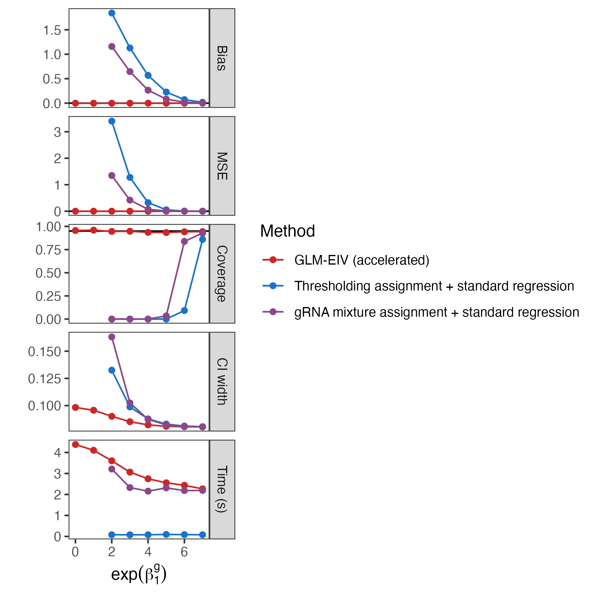
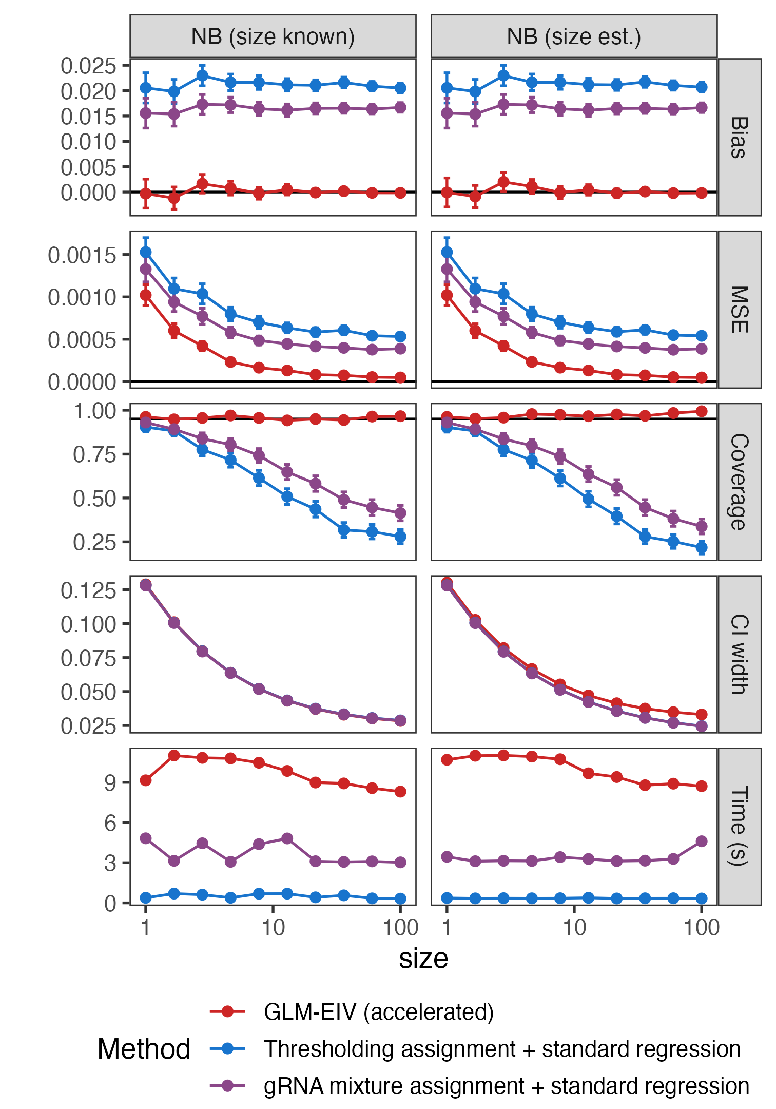
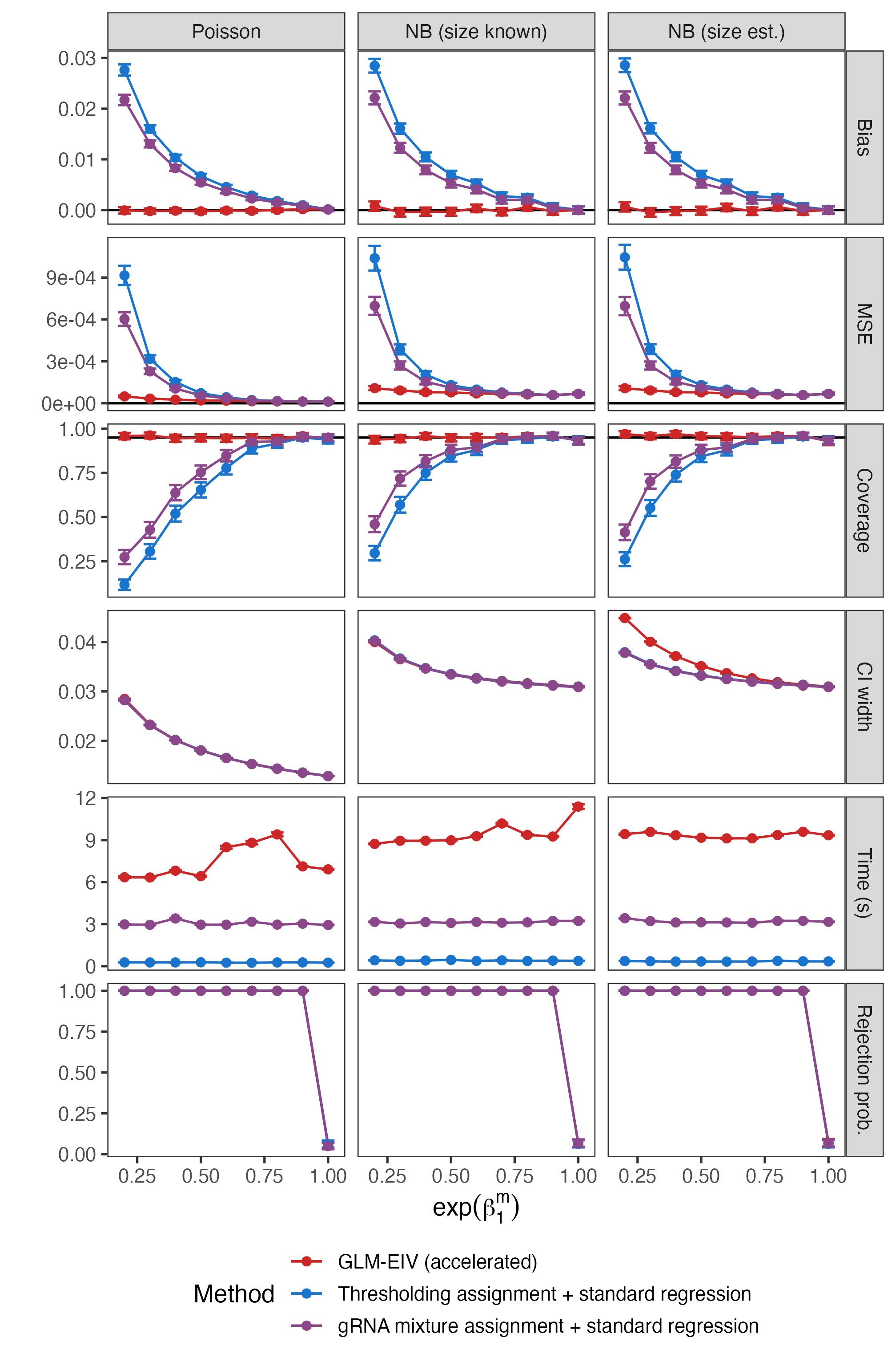
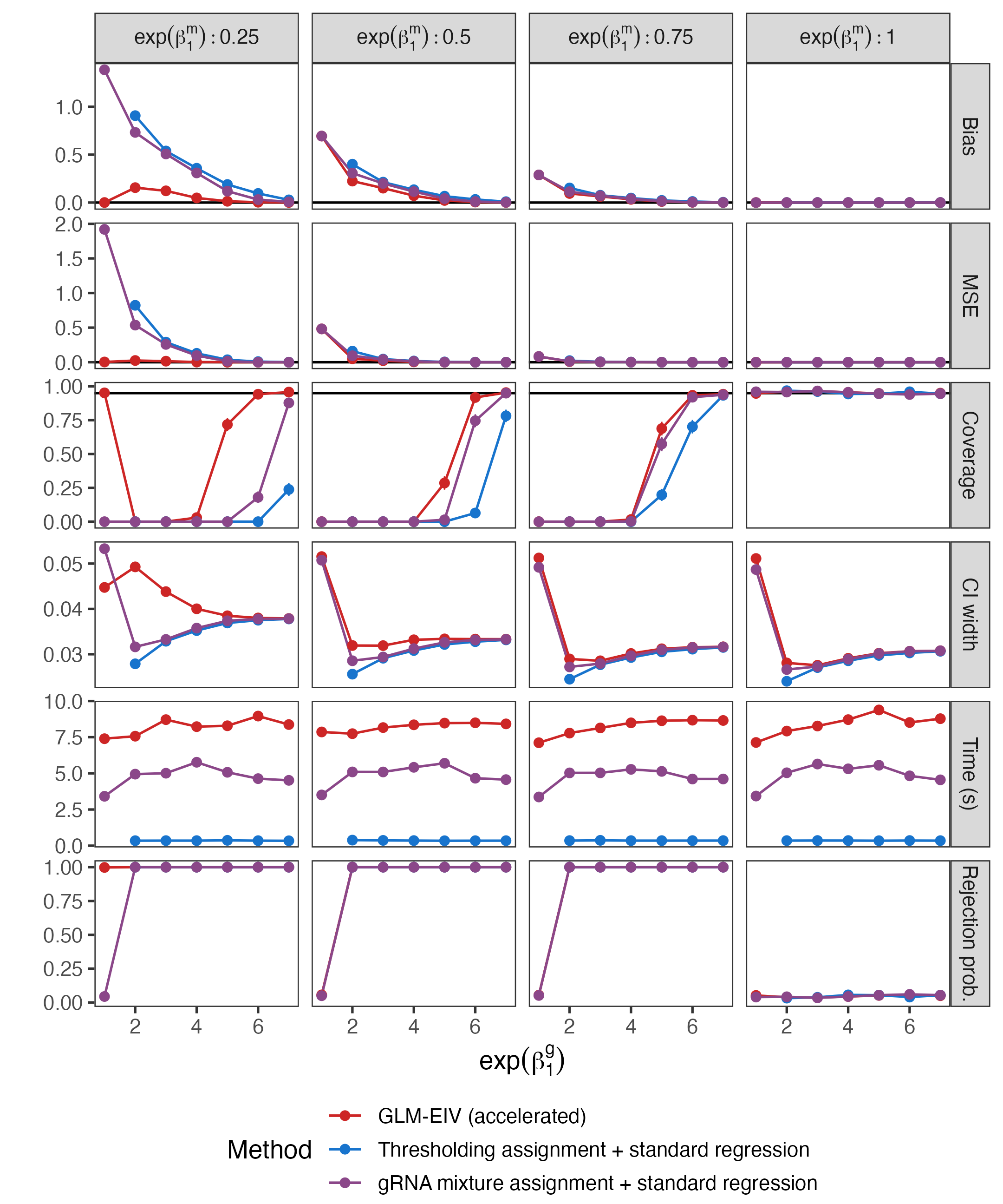
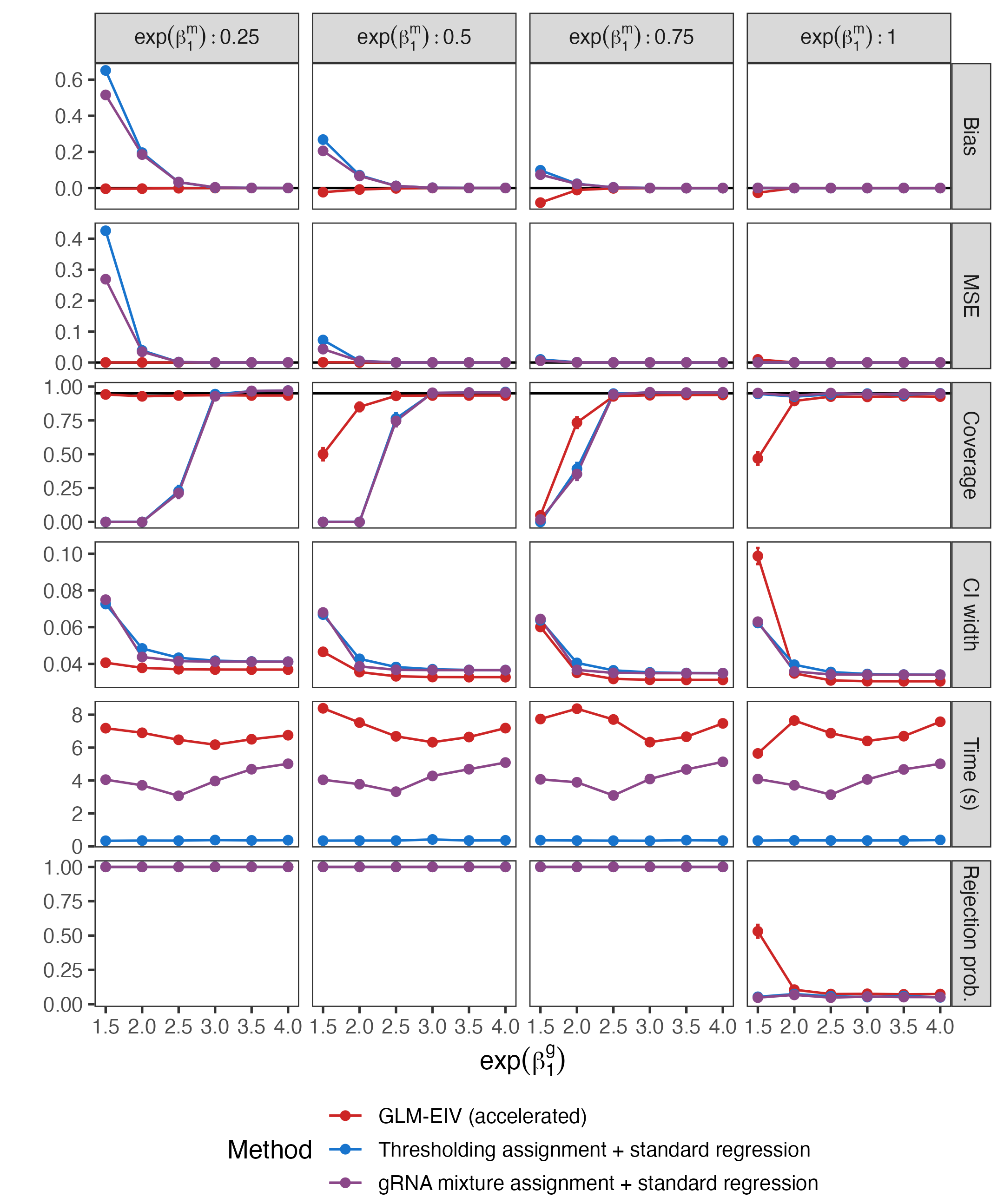
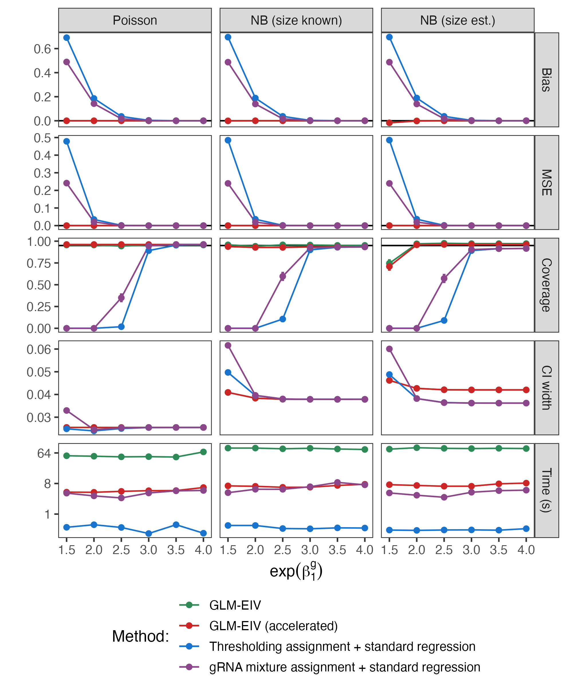
We conducted a comprehensive suite of six simulation studies to compare the empirical performance of GLM-EIV, the thresholding method, and the gRNA mixture assignment method. (We coupled the latter method to standard regression on the imputed perturbation assignments to estimate the perturbation effect size.) We describe one simulation study here and defer the remaining simulation studies to the Appendix H. We generated data on cells from the GLM-EIV model, setting the target of inference to and the probability of perturbation to . represents a decrease in gene expression by a factor of , which is a fairly large effect size on the order of what we might observe for a positive control pair. We included “sequencing batch” (modeled as a Bernoulli-distributed variable) as a covariate and sequencing depth (modeled as a Poisson-distributed variable) as an offset. We varied the log-fold change in gRNA expression, over a grid on the interval controls problem difficulty, with higher values corresponding to easier problem settings. We generated the gene expression count data from two response distributions: Poisson and negative binomial (size parameter fixed at for the latter; see simulation study 3 for an exploration of different values of ). We generated the gRNA count data from a Poisson distribution. For each parameter setting (defined by a -distribution pair), we synthesized i.i.d. datasets. Appendix H compares the parameter values used in the simulation study to those estimated from real data.
We applied four methods to the simulated data: “vanilla” GLM-EIV, accelerated GLM-EIV, thresholded regression, and the gRNA mixture assignment method. We used the Bayes-optimal decision boundary for classification as the threshold for the thresholding method (as derived in Section A.12). We ran all methods on the negative binomial data twice: once treating the size parameter as a known constant and once treating as unknown. In the latter case we used the glm.nb function from the MASS package to estimate before applying the methods (Ripley and others, 2013). We note that none of the methods accounts for the error in estimating when computing coefficient standard errors. We display the results of the simulation study in Figure 3. Columns correspond to distributions (i.e., Poisson, NB with known , and NB with unknown ), and rows correspond to performance metrics (i.e., bias, mean squared error, CI coverage rate (nominal rate ), CI width, and method run time). The parameter is plotted on the horizontal axis, and the methods are depicted in different colors. (GLM-EIV is masked by accelerated GLM-EIV in several panels).
We found that GLM-EIV outperformed the gRNA mixture method and that the gRNA mixture method outperformed thresholded regression across the metrics of bias, mean squaured error, and confidence interval coverage. We reasoned that GLM-EIV outperformed the gRNA mixture method because (i) GLM-EIV leveraged information from both modalities (rather than the gRNA modality alone) to assign perturbation identities to cells, and (ii) GLM-EIV produced soft rather than hard assignments, capturing the inherent uncertainty in whether a perturbation occurred. We additionally reasoned that the gRNA mixture method outperformed thresholded regression because the gRNA mixture method better accounted for heterogeneity across cells due to the covariates. Notably, accelerated GLM-EIV performed as well as vanilla GLM-EIV on all statistical metrics (rows 1-4) despite having substantially lower computational cost (bottom row). In fact, the running time of accelerated GLM-EIV was almost within an order of magnitude of that of the thresholding method. As expected, the confidence interval coverage of the methods degraded somewhat in the negative binomial case under estimated s as opposed to known s, but this difference was not substantial. Appendix H presents additional simulation studies in which we generate data from a Gaussian model, vary and , and assess the performance of the methods on data containing unmeasured covariates and outliers.
7 Real data application I: estimating perturbation effects in high MOI
Leveraging our computational infrastructure, we applied GLM-EIV and the thresholding method to analyze the entire Gasperini and Xie datasets. GLM-EIV ran in under two days on both datasets, using no more than 250 processors and two gigabytes of memory per process. We report only the most important aspects of the analysis and results in the main text; full details are available in Appendix F. We set the threshold in the thresholding method to the approximate Bayes-optimal decision boundary, as our theoretical analyses and simulation studies indicated that the Bayes-optimal decision boundary is a good choice for the threshold when the gRNA count distribution is well-separated. Operating under the assumption that the effect of the perturbation on gRNA expression is similar across pairs, we leveraged the fitted GLM-EIV models to approximate the Bayes boundary in the following way: we (i) sampled several hundred gene-perturbation pairs, (ii) extracted the fitted values and from the GLM-EIV models fitted to these pairs, (iii) computed the median and across the s and s, and (iv) used and to estimate a dataset-wide Bayes-optimal decision boundary (Section A.12). We repeated this procedure on both datasets, yielding a threshold of for Gasperini and for Xie.
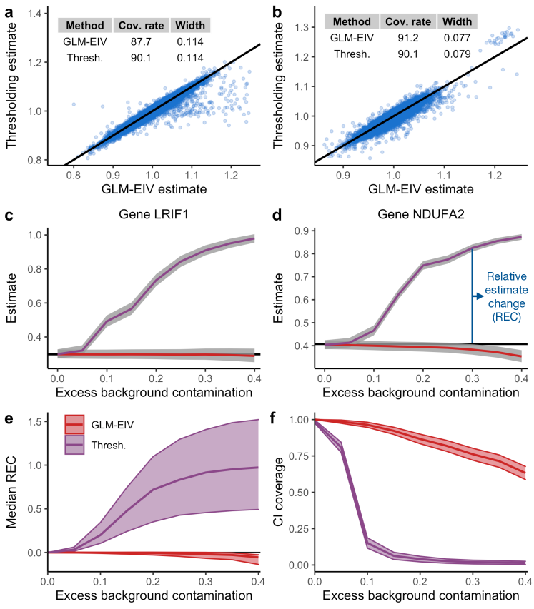
We compared GLM-EIV to thresholded regression on the real data, focusing specifically on the negative control pairs (i.e., gene-perturbation pairs for which the ground truth fold change is known to be ; Appendix F). We found that GLM-EIV and the thresholding method produced similar results (Figure 4a-b): estimates, CI coverage rates, and CI widths were concordant. CI coverage rates, which ranged from 87.7%-91.2%, were slightly below the nominal rate of 95%, likely due to mild model misspecification. The estimated effect of the perturbation on gene expression was unexpectedly large: the 95% CI for this parameter was and on the Gasperini and Xie data, respectively. We reasoned that the datasets lay in a region of the parameter space in which thresholding is a tenable strategy (provided the threshold is selected well). However, this was not obvious a priori and may not be the case for other datasets. We note that GLM-EIV produced outlier estimates (defined as estimated fold change or ) on a small ( on Gasperini, on Xie) number of pairs consisting of a handful of genes, likely due to non-global EM convergence. These outliers are not plotted in Figures 4a-b but were used to compute the CI coverage reported in the inset tables.
To evaluate performance of GLM-EIV versus thresholding in more challenging settings, we increased the difficulty of the perturbation assignment problem by generating partially-synthetic datasets. First, for a given pair, we sampled gRNA counts directly from the fitted GLM-EIV model. Next, to simulate elevated background contamination, we sampled gRNA counts from a slightly modified version of the fitted model in which we increased the mean gRNA expression of unperturbed cells while holding constant the mean gRNA expression of perturbed cells. We defined a parameter called “excess background contamination” (normed to take values in ) to quantify the relative distance between the unperturbed and perturbed gRNA count distributions. We held fixed the real-data gene expressions, library sizes, covariates, and fitted perturbation probabilities in all settings.
We generated partially-synthetic data in the above manner for each of the 322 positive control pairs in the Gasperini dataset, varying excess background contamination over the interval We then applied GLM-EIV and the thresholding method to analyze the data. We present results on two example pairs (the pair containing gene LRIF1 and the pair containing gene NDUFA2) in Figures 4c-d. We observed that the estimate produced by the methods on the raw data (depicted as a horizontal black line) coincided almost exactly with the estimate produced by the methods on the partially-synthetic data generated by setting excess background contamination to zero (This result replicated across nearly all pairs; average relative difference .) We additionally observed that as excess background contamination increased, the performance of thresholded regression degraded considerably while that of GLM-EIV remained stable.
We generalized the above analysis to the entire set of positive control pairs. First, for each pair we computed the “relative estimate change” (REC) as a function of excess background contamination, defined as the relative difference between the estimate at a given level of excess contamination and zero excess contamination (Figure 4d). Next, we computed the median REC across all positive control pairs (Figure 4e; upper and lower bands indicate the pointwise interquartile range of the REC). As excess background contamination increased, thresholded regression exhibited severe attenuation bias (as reflected by large median REC values); GLM-EIV, by contrast, remained mostly stable. Finally, letting denote the estimate obtained on the raw data, we computed the CI coverage of as a function of excess contamination. Under the assumption that is close to the true parameter , the CI coverage of the former is similar to that of the latter. We computed the CI coverage of by calculating each individual pair’s coverage of (across the Monte Carlo replicates) and then averaging this quantity across all pairs. GLM-EIV exhibited significantly higher CI coverage than thresholded regression as the data became increasingly contaminated (Figure 4f; bands indicate pointwise CIs). Coverage rates were slightly above the nominal level of in some settings because we covered an estimate of rather than itself, leading to mild “overfitting.” Nonetheless, this experiment was meaningful to assess the stability of both methods to elevated background contamination.
8 Real data application II: assigning perturbations to cells on low MOI data
Although our main focus in this work is on GLM-EIV, we sought to explore whether the gRNA mixture assignment method that we proposed in Section 5.3 might be an independently useful tool for assigning gRNAs to cells on real single-cell CRISPR screen data. The EM algorithm underlying our gRNA mixture assignment method is nearly identical to that of GLM-EIV; this algorithm is highly customized for speed and numerical stability on single-cell CRISPR screen data. We applied the gRNA mixture assignment method to assign gRNAs to cells on a low multiplicity-of-infection (or MOI) single-cell CRISPR screen of immune cells (Papalexi and others, 2021). We elected to assess the performance of the gRNA mixture assignment method on low MOI data because the “ground truth” gRNA-to-cell mapping is easier to ascertain in low MOI than in high MOI. The vast majority of cells in a low MOI screen contains a single perturbation, while a handful of cells contains zero or two perturbations and a negligible fraction of cells contains three or more perturbations. Thus, if a given gRNA constitutes a large fraction (say, ) of the gRNA reads in a given cell, we can confidently map that gRNA to that cell. Though not foolproof, this strategy yields a reasonable approximation to the ground truth in low MOI. (There is no analogous strategy for obtaining ground truth gRNA assignments in high MOI, as each cell in high MOI contains many gRNAs, and the number of gRNAs per cell is unknown and highly variable.)
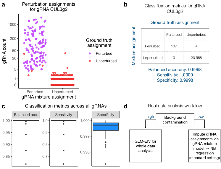
We used our proposed gRNA mixture assignment method to obtain gRNA-to-cell assignments for each gRNA in the low MOI dataset (after restricting our attention to the most highly expressed gRNAs). We included the standard technical factors as covariates, including biological replicate. We compared the mixture-model-based gRNA assignments to the ground truth assignments; the latter were obtained in the manner described above. Encouragingly, we found that these two methods produced near-identical results. For example, the mixture model determined that gRNA “CUL3g2” was present in 141 cells (and absent in the rest), while the ground truth method indicated that “CUL3g2” was present in 137 cells (Figure 5a). Treating the ground truth assignments as a reference, we constructed a confusion matrix to assess the classification accuracy of the mixture method assignments on CUL3g2 (Figure 5b). The sensitivity, specificity, and balanced accuracy of the mixture method assignments were very high (1.000, 0.9998, and 0.9998, respectively).
We replicated this analysis across the entire set of gRNAs, finding that the mixture method assignments exhibited consistently high concordance with the ground truth assignments as measured by sensitivity, specificity, and balanced accuracy (although there were a few outliers; Figure 5c). We concluded that the mixture assignment method was a statistically principled, fast, and numerically stable strategy for the recapitulating the ground truth assignments with near-optimal fidelity. We sought to compare our gRNA mixture assignment method against the Nat. Biotech. 2020 Poisson-Gaussian mixture method. Unfortunately, as discussed elsewhere (Section 5.3 and Appendix E), we were unable to get the Nat. Biotech. 2020 method (or approximations thereof written in R) working. We note that, in contrast to the Nat. Biotech. 2020 method, the proposed method allows for the inclusion of covariates (e.g., library size and batch) and models the gRNA counts directly.
9 Discussion
In this work we studied the problem of estimating the effect sizes of perturbations on changes in gene expression in high MOI single-cell CRISPR screens, focusing specifically on the challenge that the perturbation is unobserved. We showed through empirical, theoretical, and simulation analyses that the commonly-used thresholding method poses several difficulties: there exist settings (i.e., high background contamination settings) in which thresholding is not a tenable strategy, and in settings in which thresholding is a tenable strategy (i.e., low background contamination settings), selecting the optimal threshold is challenging and highly consequential. Next, we developed GLM-EIV, a method that jointly models the gene and gRNA modalities to implicitly assign perturbation identities to cells and estimate perturbation effect sizes, thereby overcoming limitations of the thresholding method. GLM-EIV demonstrated significantly improved performance relative to the thresholding method in high background contamination settings on both synthetic and realistic semi-synthetic data.
However, GLM-EIV and the thresholding method demonstrated roughly similar performance on the two real high-MOI datasets that we examined, as the real data exhibited lower background contamination than anticipated. We believe that this is an interesting finding in itself; moreover, future datasets may demonstrate higher levels of background contamination, in which case GLM-EIV will serve as an immediately usable and useful analytic tool. Finally, the gRNA mixture assignment method, which under the hood exploits the estimation machinery of GLM-EIV, is a statistically principled, numerically stable, fast, and accurate strategy for obtaining gRNA-to-cell assignments on real data; these assignments can used as input to downstream methods (e.g., negative binomial regression or SCEPTRE; Figure 5d).
We anticipate that GLM-EIV could be applied to other types of multi-modal single-cell data, such as single-cell chromatin accessibility assays. A question of interest in such experiments is whether chromatin state (i.e., closed or open) is associated with the expression of a gene or abundance of a protein (Mimitou and others, 2021). We do not directly observe the chromatin state of a cell; instead, we observe tagged DNA fragments that serve as count-based proxies for whether a given region of chromatin is open or closed. GLM-EIV might be applied in such experiments to aid in the selection of thresholds or to analyze whole datasets. The full GLM-EIV model potentially could be applied to analyze low-MOI single-cell CRISPR screen data, but we anticipate that the relative ease of assigning gRNAs to cells in low MOI (as described in section 8) may obviate the need for GLM-EIV in that setting.
The closest parallels to GLM-EIV in the statistical methodology literature are Grün and Leisch (2008) and Ibrahim (1990). Grün and Leisch derived a method for estimation and inference in a -component mixture of GLMs. While we prefer to view GLM-EIV as a generalized errors-in-variables method, the GLM-EIV model is equivalent to a two-component mixture of products of GLM densities. Ibrahim proposed a procedure for fitting GLMs in the presence of missing-at-random covariates. Our method, by contrast, involves fitting two conditionally independent GLMs in the presence of a totally latent covariate. Thus, while Ibrahim and Grün & Leisch are helpful references, our estimation and inference tasks are more complex than theirs. Next, Aigner (1973) and Savoca (2000) proposed measurement error models that consist of unobserved binary rather than continuous predictors; the latter are more commonly used in measurement error models. GLM-EIV likewise consists of a latent binary predictor, but unlike Aigner and Savoca, GLM-EIV handles a much broader class of exponential family-generated data. Finally, GLM-EIV accounts for a common source of measurement error between the predictor and response, a property not shared by classical measurement error models (Carroll and others, 2006). Additional related work is relayed in Appendix G.
GLM-EIV might be applied to areas beyond genomics, such as psychology. Many psychological constructs (e.g., presence or absence of a social media addiction) are latent and can be assessed only through an imperfect proxy (e.g., the number of times one has checked social media). Researchers might use GLM-EIV to regress an outcome variable (e.g., self-reported well-being) onto the latent construct via the imperfect proxy, potentially resolving challenges related to attenuation bias and threshold selection. Applications to psychology and other areas are a topic of future investigation.
Code and results
Results are deposited at upenn.box.com/v/glmeiv-files-v1. Github repositories containing manuscript replication code, the glmeiv R package, and the cloud/HPC-scale GLM-EIV pipeline are available at github.com/timothy-barry/glmeiv-manuscript, github.com/timothy-barry/glmeiv, and github.com/timothy-barry/glmeiv-pipeline, respectively. Detailed replication instructions are available in the first repository.
Acknowledgements
We thank Eric Tchetgen Tchetgen for helpful conversations, Xuran Wang for helping to process the Xie dataset, and Songcheng Dai for helping to deploy the GLM-EIV pipeline on Azure. This work used the Extreme Science and Engineering Discovery Environment (XSEDE; NSF grant ACI-1548562) and the Bridges-2 system (NSF grant ACI-1928147) at the Pittsburgh Supercomputing Center. This work is funded by National Institute of Mental Health (NIMH) grant R01MH123184 and NSF grant DMS-2113072.
References
- Aigner (1973) Aigner, Dennis J. (1973). Regression with a binary independent variable subject to errors of observation. Journal of Econometrics 1(1), 49–59.
- Barry and others (2021) Barry, Timothy and others. (2021). SCEPTRE improves calibration and sensitivity in single-cell CRISPR screen analysis. Genome Biology, 1–19.
- Candès and others (2018) Candès, Emmanuel and others. (2018). Panning for gold: ‘model-X’ knockoffs for high dimensional controlled variable selection. Journal of the Royal Statistical Society. Series B: Statistical Methodology 80(3), 551–577.
- Carroll and others (2006) Carroll, Raymond J and others. (2006). Measurement error in nonlinear models: a modern perspective. Chapman and Hall/CRC.
- Choudhary and Satija (2022) Choudhary, Saket and Satija, Rahul. (2022). Comparison and evaluation of statistical error models for scrna-seq. Genome biology 23(1), 1–20.
- Datlinger and others (2017) Datlinger, Paul and others. (2017). Pooled CRISPR screening with single-cell transcriptome readout. Nature Methods 14(3), 297–301.
- Fitzpatrick (2009) Fitzpatrick, Patrick. (2009). Advanced calculus, Volume 5. American Mathematical Soc.
- Gallagher and Chen-Plotkin (2018) Gallagher, Michael D. and Chen-Plotkin, Alice S. (2018). The Post-GWAS Era: From Association to Function. American Journal of Human Genetics 102(5), 717–730.
- Gasperini and others (2019) Gasperini, Molly and others. (2019). A Genome-wide Framework for Mapping Gene Regulation via Cellular Genetic Screens. Cell 176(1-2), 377–390.e19.
- Grün and Leisch (2008) Grün, Bettina and Leisch, Friedrich. (2008). Finite Mixtures of Generalized Linear Regression Models. Heidelberg: Physica-Verlag HD, pp. 205–230.
- Hafemeister and Satija (2019) Hafemeister, Christoph and Satija, Rahul. (2019). Normalization and variance stabilization of single-cell RNA-seq data using regularized negative binomial regression. Genome Biology 20(1), 1–15.
- Hill and others (2018) Hill, Andrew J. and others. (2018). On the design of CRISPR-based single-cell molecular screens. Nature Methods 15(4), 271–274.
- Ibrahim (1990) Ibrahim, Joseph G. (1990). Incomplete Data in Generalized Linear Models. Journal of the American Statistical Association 85(411), 765–769.
- Lin and others (2021) Lin, Kevin Z., Lei, Jing and Roeder, Kathryn. (2021). Exponential-Family Embedding With Application to Cell Developmental Trajectories for Single-Cell RNA-Seq Data. Journal of the American Statistical Association 0(0), 1–32.
- Liu and others (2021) Liu, Molei and others. (2021). Fast and Powerful Conditional Randomization Testing via Distillation. Biometrika, 1–25.
- Louis (1982) Louis, By Thomas A. (1982). Finding the Observed Information Matrix when Using the EM Algorithm. Society 44(2), 226–233.
- McCullagh and Nelder (1990) McCullagh, P. and Nelder, J. A. (1990). Generalized Linear Models, 2nd Edn.
- Mimitou and others (2021) Mimitou, Eleni P. and others. (2021). Scalable, multimodal profiling of chromatin accessibility, gene expression and protein levels in single cells, Volume 39. Springer US.
- Morris and others (2023) Morris, John A, Caragine, Christina, Daniloski, Zharko, Domingo, Júlia, Barry, Timothy, Lu, Lu, Davis, Kyrie, Ziosi, Marcello, Glinos, Dafni A, Hao, Stephanie and others. (2023). Discovery of target genes and pathways at gwas loci by pooled single-cell crispr screens. Science 380(6646), eadh7699.
- Musunuru and others (2021) Musunuru, Kiran and others. (2021). In vivo CRISPR base editing of PCSK9 durably lowers cholesterol in primates. Nature 593(7859), 429–434.
- Papalexi and others (2021) Papalexi, Efthymia, Mimitou, Eleni P, Butler, Andrew W, Foster, Samantha, Bracken, Bernadette, Mauck III, William M, Wessels, Hans-Hermann, Hao, Yuhan, Yeung, Bertrand Z, Smibert, Peter and others. (2021). Characterizing the molecular regulation of inhibitory immune checkpoints with multimodal single-cell screens. Nature genetics 53(3), 322–331.
- Przybyla and Gilbert (2021) Przybyla, Laralynne and Gilbert, Luke A. (2021). A new era in functional genomics screens. Nature Reviews Genetics.
- Replogle and others (2020) Replogle, Joseph M. and others. (2020). Combinatorial single-cell CRISPR screens by direct guide RNA capture and targeted sequencing. Nature Biotechnology.
- Ripley and others (2013) Ripley, Brian and others. (2013). Package ‘mass’. Cran r 538, 113–120.
- Sarkar and Stephens (2021) Sarkar, Abhishek and Stephens, Matthew. (2021). Separating measurement and expression models clarifies confusion in single-cell RNA sequencing analysis. Nature Genetics 53(6), 770–777.
- Savoca (2000) Savoca, E. (2000). Measurement errors in binary regressors: An application to measuring the effects of specific psychiatric diseases on earnings. Health Services and Outcomes Research Methodology 1(2), 149–164.
- Stefanski (2000) Stefanski, L. A. (2000). Measurement Error Models. Journal of the American Statistical Association 95(452), 1353–1358.
- Townes and others (2019) Townes, F. William and others. (2019). Feature selection and dimension reduction for single-cell RNA-Seq based on a multinomial model. Genome Biology 20(1), 1–16.
- Trapnell and others (2014) Trapnell, Cole and others. (2014). The dynamics and regulators of cell fate decisions are revealed by pseudotemporal ordering of single cells. Nature Biotechnology 32(4), 381–386.
- Xie and others (2019) Xie, Shiqi and others. (2019). Global Analysis of Enhancer Targets Reveals Convergent Enhancer-Driven Regulatory Modules. Cell Reports 29(9), 2570–2578.e5.
Appendices
Appendix A Theoretical details for thresholding estimator
We study the thresholding method from a theoretical perspective, recovering in a simplified Gaussian setting phenomena revealed in the empirical analysis. Suppose we observe gRNA expression and gene expression data on cells from the following linear model:
| (7) |
where and are independent. For a given threshold , the imputed perturbation assignment is The thresholding estimator is the OLS solution, i.e. We derive the almost sure limit of :
Proposition 1.
The almost sure limit (as ) of is
| (8) |
where , , and
The function does not depend on the gene expression parameters or . The asymptotic relative bias of is given by
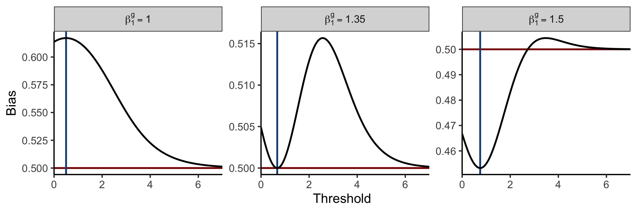
Having derived an exact expression for the asymptotic relative bias of , we can prove several results about this quantity. We fix to for simplicity. (In reality, is smaller, but the relevant statistical phenomena emerge for .) We start with informal proposition statements; we follow up with formal proposition statements below. First, the thresholding estimator strictly underestimates (in absolute value) the true value of over all choices of the threshold and over all values of the regression coefficients and . This phenomenon, called attenuation bias, is a common attribute of estimators that ignore measurement error in errors-in-variables models (Stefanski, 2000). Second, the magnitude of the bias decreases monotonically in , comporting with the intuition that the problem becomes easier as the gRNA mixture distribution becomes increasingly well-separated. Third, the Bayes-optimal decision boundary (i.e., the most accurate decision boundary for classifying cells) is a critical value of the bias function. Finally, and most subtly, there is no universally applicable rule for selecting a threshold that yields minimal bias: when is small, setting the threshold to an arbitrarily large number yields smaller bias than setting the threshold to the Bayes decision boundary; when is large, the reverse is true.
We state five propositions labeled 2 – 6 corresponding to the informal claims above; these propositions are depicted visually in Figure 6.
Proposition 2.
Fix . For all , the asymptotic relative bias is positive, i.e.
Proposition 3.
Fix . The asymptotic relative bias decreases monotonically in , i.e.
Let denote the Bayes-optimal decision boundary for classifying cells as perturbed or unperturbed, i.e. for . We have that is a critical value of the bias function:
Proposition 4.
For and given , the Bayes-optimal decision boundary is a critical value of the bias function , i.e.
Furthermore, as the threshold tends to infinity, the asymptotic relative bias tends to :
Proposition 5.
Assume without loss of generality that . As the threshold tends to infinity, the asymptotic relative bias tends to i.e.
As a corollary, when , asymptotic relative bias tends to as tends to infinity. Finally, we compare two threshold selection strategies head-to-head: setting the threshold to an arbitrarily large number, and setting the threshold to the Bayes-optimal decision boundary:
Proposition 6.
Assume without loss of generality that . For , we have that
For , we have that
Finally, for , we have that
In other words, setting the threshold to a large number yields a smaller bias when is small (i.e., ; Figure 7a, left); setting the threshold to the Bayes-optimal decision boundary yields a smaller bias when is large (i.e., ; Figure 7a, right); and the two approaches coincide when is intermediate (i.e., ; Figure 7a, middle).
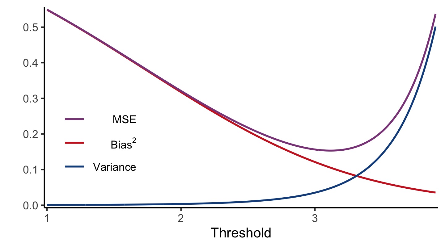
Next, we study the variance of the thresholding estimator, considering a slightly simpler model for this purpose. Suppose the intercepts in (7) are fixed at (i.e., = = 0). For notational simplicity we write and The thresholding estimator is the no-intercept OLS solution The following proposition derives the scaled, asymptotic distribution of
Proposition 7.
The limiting distribution of is
where
This proposition yields an asymptotically exact bias-variance decomposition for : as the threshold tends to infinity, the bias decreases and the variance increases. Figure 7 plots the bias-variance decomposition as a function of the threshold.
A.1 Organization
The following subsections prove all propositions. Section A.2 introduces some notation. Section A.3 establishes almost sure convergence of the thresholding estimator in the model (7), proving Proposition 1. Section A.4 simplifies the expression for the attenuation function , and section A.5 computes derivatives of to be used throughout the proofs. Section A.6 establishes the limit in of , proving Proposition 5. Section A.7 establishes that the Bayes-optimal decision boundary is a critical value of , proving Proposition 4, and section A.8 compares the competing threshold selection strategies head-to-head, proving Proposition 6. Section A.9 demonstrates that is monotone in , proving Proposition 3, and Section A.10 establishes attenuation bias of the thresholding estimator, proving Proposition 2. Finally, Section A.11 derives the bias-variance decomposition of the thresholding estimator in the no-intercept version of 7, proving Proposition 7.
A.2 Notation
All notation introduced in this subsection (i.e., A.2) pertains to the Gaussian model with intercepts (7). Recall that the attenuation function is defined by
where
Additionally, recall that the asymptotic relative bias function is Next, we define the functions and by
| (9) |
and
| (10) |
We use to denote the density, and we denote the right-tail probability probability of by , i.e.,
The parameter is a given, fixed constant throughout the proofs. Therefore, to minimize notation, we typically use (resp., ) to refer to the function (resp., ) evaluated at . Finally, for a given function , point , and index , we use the symbol to refer to the derivative of the th argument of evaluated at (sensu Fitzpatrick (2009)). For example, is the derivative of the first argument of (the argument corresponding to ) evaluated at . Likewise, is the derivative of the second argument of (the argument corresponding to ) evaluated at
A.3 Almost sure limit of
We derive the limit in probability of for the Gaussian model with intercepts (7). Dividing by in (8), we can express as
By weak LLN, To compute this quantity, we first compute several simpler quantities:
-
1.
Expectation of :
-
2.
Expectation of :
-
3.
Expectation of :
-
4.
Expectation of :
-
5.
Variance of : Because is binary, we have that
-
6.
Covariance of :
Combining these expressions, we have that
A.4 Re-expressing in a simpler form
We rewrite the attenuation fraction in a way that makes it more amenable to theoretical analysis. We leverage the fact that integrates to unity and is even. We have that
| (11) |
and so
| (12) |
Next,
| (13) |
and so
| (14) |
Combining (11, 12, 13, 14), we find that
| (15) |
As a corollary, when ,
| (16) |
Recalling the definitions of (9) and (10), we can write as
The special case (16) is identical to
| (17) |
i.e., the numerator and denominator of (17) coincide with those of (16). We sometimes will use the notation and to refer to the numerator and denominator of (16), respectively.
A.5 Derivatives of and in
We compute the derivatives of and in , which we will need to prove subsequent results. First, by the FTC (fundamental theorem of calculus) and the evenness of , we have that
| (18) |
Second, we have that
| (19) |
A.6 Limit of in
Assume (without loss of generality) that . We compute . Observe that
Therefore, we can apply L’Hôpital’s rule. We have by (18) and (19) that
| (20) |
We evaluate the two terms in the product (20) separately. Dividing by , we see that
| (21) |
To evaluate the limit of (21), we first evaluate the limit of
| (22) |
Taking the limit in (22), we obtain
for . We now can evaluate the limit of (21):
Next, we compute the limit of the other term in the product (20):
| (23) |
Combining (21) and (23), the limit (20) evaluates to
It follows that the limit in of the asymptotic relative bias is
A corollary is that
A.7 Bayes-optimal decision boundary as a critical value of
A.8 Comparing Bayes-optimal decision boundary and large threshold
We compare the bias produced by setting the threshold to a large number to the bias produced by setting the threshold to the Bayes-optimal decision boundary. Let be the value of attenuation function evaluated at the Bayes-optimal decision boundary , i.e.
We set to and solve for :
Because is a strictly increasing function, it follows that for and for Next, because
we have that for and for . Recall that the bias induced by sending the threshold to infinity (as stated in Proposition 5 and proven in Section A.6) is , i.e.
We conclude that on ; for ; and on .
A.9 Monotonicity in
We show that is monotonically increasing in for and given threshold . We begin by stating and proving two lemmas. The first lemma establishes an inequality that will serve as the basis for the proof.
Lemma A.1.
The following inequality holds:
| (27) |
Proof: We take cases on the sign on .
Case 1: . Then implying or Moreover, is positive. Therefore, the right-hand side of (27) is negative.
Turning our attention of the left-hand side of (27), we see that
| (28) |
Additionally, and . Combining these facts with (28), we find that
Finally, because the entire left-hand side of (27) is positive. The inequality holds for .
Case 2: We will show that the first term on the LHS of (27) is greater than the first term on the RHS of (27), and likewise that the second term on the LHS is greater than the second term on the RHS, implying the truth of the inequality. Focusing on the first term, the positivity of implies that and so
Next, focusing on the second term, implies that
| (29) |
Adding to both sides of (29) yields
The inequality holds for . Combining the cases, the inequality holds for all .
The second lemma establishes the derivatives of the functions and in .
Lemma A.2.
The derivatives in of and are
| (30) |
| (31) |
Proof: Apply FTC and product rule.
We are ready to prove the monotonicity of in . Subtracting
from both sides of (27) and multiplying by yields
| (32) |
Next, recall that
| (33) |
and
| (34) |
Substituting (30, 31, 33, 34) into (32) produces
or
| (35) |
The quotient rule implies that
| (36) |
We conclude by (35) and (36) that is monotonically increasing in . Finally, is monotonically decreasing in .
A.10 Strict attenuation bias
A.11 Bias-variance decomposition in no-intercept model
We prove the bias-variance decomposition for the no-intercept version of (7). Define (for “limit”) by
where
We have that
Therefore,
| (37) |
Next, we compute the expectation and variance of . To do so, we first compute several simpler quantities:
-
1.
Expectation of :
-
2.
Expectation of :
-
3.
Expectation of :
-
4.
Expectation of :
A.12 Bayes-optimal decision boundary for non-Gaussian mixture distributions and GLMs
We report the Bayes-optimal decision boundary for gRNA count distributions that are non-Gaussian. First, consider a simple two-component Poisson mixture model with means and and mixing probability :
where is a Poisson density. Suppose we draw an observation from this distribution. The Bayes-optimal threshold for classifying the observation as having been drawn from the first or second component is
| (42) |
Next, consider the slightly more complex Poisson mixture GLM:
where is unobserved. Conditional on the covariates and offset, the mean of the unperturbed component is and that of the perturbed component is The Bayes-optimal threshold is obtained by plugging in for and for in (42). To obtain a fixed gRNA assignment threshold across cells, we compute the Bayes-optimal decision boundary for each cell and then take the average across cells. The situation is similar for the negative binomial (with known size ) distribution; the Bayes-optimal decision boundary in this case is
Appendix B Estimation and inference in the GLM-EIV model
B.1 Detailed specification of the model
We provide a more precise and technical specification of the GLM-EIV model than provided in the main text. Let be the vector of covariates (including an intercept term) for the th cell. (We use the tilde as a reminder that the vector is partially unobserved.) Let and be the unknown coefficient vectors corresponding to the gene and gRNA expression models, respectively. Finally, let and be the (possibly zero) offset terms for the gene and gRNA models; in practice, we typically set and to the log-transformed library sizes (i.e., and , respectively).
We use a pair of GLMs to model the gene and gRNA expressions. Considering first the gene expression model, let the th linear component of the model be Next, let the mean of the th observation be where is a strictly increasing, differentiable link function. Let be the differentiable, cumulant-generating function of the selected exponential family distribution. We can express the canonical parameter in terms of and by Finally, let be the carrying density of the selected exponential family distribution. The density of conditional on the the canonical parameter is We implicitly set the “scale” term (i.e., the term in McCullagh and Nelder (1990), Eqn. 2.4, p. 28) to unity; this slightly simplified model encompasses the most important distributions for our purposes, including the Poisson, negative binomial, and Gaussian (with unit variance) distributions.
Let the terms and be defined in an analogous way for the gRNA model, i.e. , , and The density of given the canonical parameter is Finally, the unobserved variable is assumed to follow a Bernoulli distribution with mean . Its marginal density is given by The unknown parameters in the model are
B.2 Notation
We briefly introduce notation that we will use throughout. For , let denote the value of that results from setting to . Next, let , and be the values of , , and , respectively, that result from setting to , i.e., , , and Let the corresponding gRNA quantities , , and be defined analogously. Next, let be the observed design matrix, and let be the augmented design matrix that results from concatenating the column of (unobserved) s to , i.e.
Furthermore, for , let be the matrix that results from setting to for all in , and let denote the matrix that results from vertically concatenating and . Furthermore, define , and let , , , and be defined analogously. Finally, let be the vector that results from concatenating to itself, i.e. and let , , and be defined similarly.
B.3 Log likelihood and estimation
We conduct estimation and inference conditional on the library sizes and technical factors and ; therefore, we treat these quantities as fixed constants. We assume that the gene expression and gRNA expression are conditionally independent given the perturbation . The model log-likelihood is
| (43) |
We see from (43) that the GLM-EIV model is equivalent to a two-component mixture of products of GLM densities. We estimate the parameters of the GLM-EIV model using an EM algorithm.
E step
The E step entails computing the membership probability of each cell. Let be the parameter estimate at the -th iteration of the algorithm. For , let be the th canonical parameter at the -th iteration of the algorithm of the gene expression distribution that results from setting to , i.e. Similarly, let be defined by Next, for define by
Finally, let and . The th membership probability is
| (44) |
where we set
| (45) |
Next, we have that
We therefore conclude that which is easily computable.
M step
The complete-data log-likelihood of the GLM-EIV model is
| (46) |
Define We have that
| (47) |
The three terms of (47) are functions of different parameters: the first is a function of the second is a function of and the third is a function of . Therefore, to find the maximizer of (47), we maximize the three terms separately. Differentiating the first term with respect to , we find that
Setting the derivative equal to and solving for ,
Thus, the maximizer of (47) in is . Next, define . We can view the second term of (47) as the log-likelihood of a GLM – call it – that has exponential family density , link function , responses , offsets , weights , and design matrix Therefore, the maximizer of the second term of (47) is the maximizer of , which we can compute using the iteratively reweighted least squares (IRLS) procedure, as implemented in R’s GLM function. Similarly, the maximizer of the third term of (47) is the maximizer of the GLM with exponential family density , link function , responses , offsets , weights , and design matrix
B.4 Inference
We derive the asymptotic observed information matrix of the GLM-EIV log likelihood, enabling us to perform inference on the parameters. First, we define some notation. For , , and let be defined by
Let the matrix be given by Next, define the diagonal matrices , , , and by
Define the matrices and analogously. These matrices are unobserved, as they depend on . Next, for , let the diagonal matrices and be given by
Define the matrices , , and analogously. Finally, define the vectors by
and let the vectors and be defined analogously. The quantities and are all observed.
The observed information matrix evaluated at is the negative Hessian of the log likelihood (43) evaluated at , i.e. This quantity, unfortunately, is hard to compute, as the log likelihood (43) is a complicated mixture. Louis (1982) showed that is equivalent to the following quantity:
| (48) |
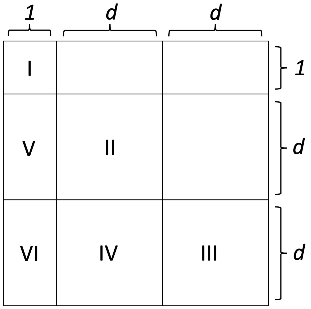
The observed information matrix has dimension Recall that the complete-data log-likelihood (46) is the sum of three terms. The first term depends only on , the second on , and the third on . Therefore, the observed information matrix can be viewed as block matrix consisting of nine submatrices (Figure 8; only six submatrices labelled). Submatrix I depends on , submatrix II on , submatrix III on , submatrix IV on and , submatrix V on and , and submatrix VI on and . We only need to compute these six submatrices to compute the entire matrix, as the matrix is symmetric. The following sections derive formulas for submatrices I-VI. All expectations are understood to be conditional on and . The notation and represent the gradient and Hessian, respectively, with respect to the vector .
Submatrix I
Denote submatrix I by The formula for is
| (49) |
We begin by calculating the first and second derivatives of the log-likelihood with respect to . The first derivative is
| (50) |
The second derivative is
We compute the expectation of the first term of (49):
| (51) |
Next, we compute the difference of the second two pieces of (49). To this end, define and We have that
Next,
Therefore,
| (52) |
Stringing (49), (51) and (52) together, we obtain
| (53) |
Submatrix II
Denote submatrix II by The formula for is
| (54) |
Standard GLM results imply that and We compute the first term of (54). The th entry of this matrix is
We therefore have that
| (55) |
Next, we compute the difference of the last two terms of (54). The th entry is
The sum of the last two terms on the right-hand side of (54) is therefore
| (56) |
Combining (54), (55), (56), we find that
| (57) |
Submatrix III
Denote submatrix III by The formula for sub-matrix III is similar to that of sub-matrix II (57). Substituting for in this equation yields
| (58) |
Submatrix IV
Denote sub-matrix IV by . The formula for is
| (59) |
First, we have that
| (60) |
as differentiating with respect to yields a vector that is a function of , and differentiating this vector with respect to yields . Next, recall from GLM theory that and The th entry of the last two terms of (59) is
| (61) |
Combining (59), (60), and (61) produces
| (62) |
Submatrix V
Submatrix VI
Denote submatrix VI by Calculations similar to those for submatrix V show that
| (67) |
Combining submatrices
To summarize, the formulas for submatrices I-VI are as follows:
-
I
-
II
-
III
-
IV
-
V
-
VI
We stitch these pieces together and transpose submatrices IV, V, and VI to produce the whole information matrix . Evaluating this matrix at the EM estimate and inverting yields the asymptotic covariance matrix, which we can use to compute standard errors.
B.5 Implementation
To evaluate the observed information matrix, we need to compute the matrices and and the vectors and for . We likewise need to compute the analogous gRNA quantities. The procedure that we propose for this purpose is general, but for concreteness, we describe how to implement this procedure using the glm function in R by extending base family objects. We implicitly condition on , , and .
An R family object contains several functions, including linkinv, variance, and mu.eta. linkinv is the inverse link function . variance takes as an argument the mean of the th example and returns its variance . mu.eta is the derivative of the inverse link function . We extend the R family object by adding two additional functions: skewness and mu.eta.prime. skewness returns the skewness of the distribution as a function of the mean , i.e.
Finally, mu.eta.prime is the second derivative of the inverse link function Algorithm 2 computes the matrices , , , and and vector for given and given family object. (The vector can be computed in terms of and .) We use (resp. ) to refer to the standard deviation (resp. skewness) of the gene expression distribution the th cell when the perturbation is set to .
All steps of the algorithm are obvious except the calculation of (line 6), (line 9), and (line 12). We omit the notation for compactness. First, we prove the correctness of the expression for . Recall the basic GLM identities
| (68) |
and, for all ,
| (69) |
Differentiating (69) in , we find that
| (70) |
Finally, plugging in for ,
Next, we prove the correctness for the expression for . Recall the exponential family identity
| (71) |
Differentiating (70) in , we obtain
Plugging in for , we find that
Finally, the expression for follows from (68). We can apply a similar algorithm to compute the analogous matrices for the gRNA modality. Table 1 shows the linkinv, variance, mu.eta, skewness, and mu.eta.prime functions for several common family objects (which are defined by a distribution and link function).
| Gaussian response, identity link | Poisson response, log link | NB response ( fixed), log link | |
|---|---|---|---|
| linkinv | |||
| variance | |||
| mu.eta | |||
| skewness | |||
| mu.eta.prime |
Appendix C Zero-inflated model
In this section we introduce the “zero-inflated” GLM-EIV model. The zero-inflated GLM-EIV model is appropriate to use when the unperturbed cells do not transcribe any gRNA molecules (i.e., when there are no background reads). Let be the vector of observed covariates, including an intercept term. ( is the same as , but with the perturbation indicator removed.) Let be an unknown coefficient vector. ( is the same as , but with the perturbation effect removed). Let the linear component , mean , and canonical parameter of gRNA count distribution of the th cell be given by
The density of gRNA counts in the zero-inflated model is as follows:
In other words, when the cell is perturbed (i.e., ), the zero-inflated density coincides with the background-read density ; by contrast, when the cell is unperturbed (i.e., ), the zero-inflated density is a point mass at zero. The gene expression density and perturbation indicator density are the same across the background read and zero-inflated models. We assume that the gene expression and gRNA count are conditionally independent given the perturbation indicator . The joint density of is
The complete-data log-likelihood is
where is the vector of unknown parameters. Integrating over the unobserved variable , the marginal of is
Finally, the log-likelihood is
C.1 Estimation
To estimate the parameters of the zero-inflated GLM-EIV model, we use an EM algorithm similar to Algorithm 1 but with two changes. First, we use a different formula for the th membership probability at the -th step of the algorithm . (We use to denote the th membership probability in both the background read and zero inflated cases; the difference should be clear from context.) Let be the parameter estimate at the -th iteration of the algorithm. Arguing in a manner similar to the background read case, we have that
where
The expression for is
where Notice that if , then This comports with our intuition that a nonzero gRNA count indicates the presence of a perturbation.
Next, we consider the M step of the EM algorithm, which is similar to the background read case. Define We have that
| (72) |
The three terms of (72) are functions of , , and , respectively. The maximizer and of the first and second term are the same as in the background read case. The maximizer of the third term is the maximizer of the GLM with exponential family density , link function , responses , weights , design matrix , offsets .
C.2 Inference
Next, we derive the asymptotic observed information matrix for the zero-inflated model, allowing us to perform inference. Again, let but note that is computed differently than in the background read case. Define the matrices and by
Also, define the vectors and by
and
These quantities are computable, as they do not depend on the unobserved variables . Finally, let the unobserved, matrix be defined by .
The observed information matrix is given by Louis’s theorem implies that
The matrix has dimension and consists of nine submatrices (Figure 9). Three of these submatrices (i.e., I, II, and V) are the same as the corresponding submatrices in the background read case. We therefore must compute the remaining submatrices (i.e., III, IV, and VI) to compute the entire matrix . Again, in the following, all expectations are understood to be conditional on and .
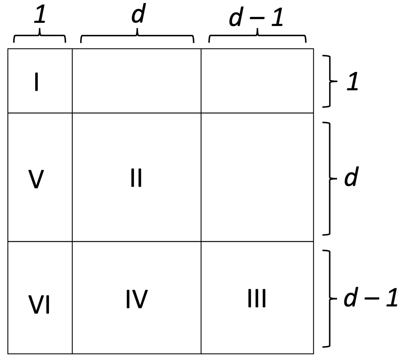
Submatrix III (zero-inflated)
Denote submatrix III by The formula for is
| (73) |
GLM theory indicates that and We begin by computing the first term of (73). The only random matrix among , , , and is . Therefore, by the linearity of expectation,
| (74) |
Next, we compute the difference of the last two terms of (73). The th entry of this matrix is
Therefore, we have that
| (75) |
Combining (73), (74), and (75), we conclude that
| (76) |
Submatrix IV (zero-inflated)
Denote submatrix IV by . The formula for submatrix IV is
| (77) |
First, we have that
| (78) |
as the derivative in of is a function of , and the derivative in of this term is . Next, we compute the difference of the last two terms of (77). Entry of this matrix is
| (79) |
Combining (73), (74), and (75) yields
| (80) |
Submatrix VI (zero-inflated)
Denote submatrix VI by The formula for is
| (81) |
Recall that and where and We have that
| (82) |
as the derivative in of is a function of , and the derivative in of this term is . Next, we compute the difference of the second two terms of (81). The th entry of this vector is
| (83) |
Combining (81), (82), and (83), we conclude that
| (84) |
Appendix D Statistical accelerations and computing
D.1 Statistical accelerations
We describe in detail the procedure for obtaining the pilot parameter estimates . This procedure consists of two subroutines, which we label Algorithm 3 and Algorithm 4. The first step (Algorithm 3) is to obtain good parameter estimates for and via regression. Recall that the underlying gene expression parameter vector is , where is the intercept, is the effect of the perturbation, and is the effect of the technical factors. To produce estimates and , we regress the gene expressions onto the technical factors . The intuition for this procedure is as follows: the probability of perturbation is very small. Therefore, the true log likelihood is approximately equal to the log likelihood that results from omitting from the model:
We similarly can obtain pilot estimates and by regressing the gRNA counts onto the technical factors . We extract the fitted values (on the scale of the linear component) for use in a subsequent step: for .
| Fit a GLM with responses , offsets , design matrix , distribution , and link function . |
Next, we obtain estimates and for , , and by fitting a “reduced” GLM-EIV (Algorithm 4). The log likelihood of the no-intercept, univariate GLM with predictor and offset is approximately equal to the true log likelihood:
| Fit no-intercept, univariate GLM with predictors , responses , offsets and weights . |
| Compute log likelihood currLik using ,, and |
Therefore, to estimate , , and , we fit a GLM-EIV model with gene expressions , gRNA counts , gene offsets , gRNA offsets , and no intercept or covariate terms. Intuitively, we “encode” all information about technical factors, library sizes, and baseline expression levels into and . We run the algorithm times over randomly-selected starting values for , , and and select the solution with greatest the log likelihood.
The M step of the reduced GLM-EIV algorithm requires fitting two no-intercept, univariate GLMs with offsets. We derive analytic formulas for the MLEs of these GLMs in the three most important cases: Gaussian response with identity link, Poisson response with log link, and negative binomial response with log link (see section D.2; the latter formula is asymptotically exact). Consequently, we do not need to run the relatively slow IRLS procedure to carry out the M step of the reduced GLM-EIV algorithm. Overall, the proposed method for obtaining the full set of pilot parameter estimates requires fitting only two GLMs (via IRLS).
D.2 Intercept-plus-offset models
A key step in the algorithm for computing the pilot parameter estimates (Algorithm 4) is to fit a weighted, no-intercept, univariate GLM with nonzero offset terms and a binary predictor variable. We derive an analytic formula for the MLE of this GLM for three important pairs of response distributions and link functions: Gaussian response with identity link, Poisson response with log link, and negative binomial response with log link. The GLM that we seek to estimate has responses , predictors , offsets and weights Throughout, denotes a universal constant. The log likelihood of this GLM is
| (85) |
Thus, finding the MLE is equivalent to estimating a GLM with intercept , offsets , weights , and no covariate terms. We term such a GLM a intercept-plus-offset model. Below, we study intercept-plus-offset models in generality.
General formulation
Let be an unknown constant. Let , where is a distribution. Let be exponential family-distributed random variables with identity sufficient statistic. Suppose the mean of is given by where is a strictly increasing, differentiable link function. We call this model the intercept-plus-offset model.
We derive the (weighted) log likelihood of this model. Let be weights, where is a distribution bounded above by and below by . (A special case, which corresponds to no weights, is for all .) Throughout, we assume that and have finite first moment. Suppose the cumulant-generating function and carrying density of the exponential family distribution are and , respectively. The canonical parameter of the th observation is
| (86) |
and the density of is The weighted log likelihood is
| (87) |
Our goal is to find the weighted MLE of . We consider three important choices for the exponential family distribution and link function. In the first two cases – Gaussian distribution with identity link and Poisson distribution with log link – we find the finite-sample maximizer of (87); by contrast, in the third case – negative binomial distribution with log link – we find an asymptotically exact maximizer.
Gaussian
Poisson
Negative binomial
Finally, we consider a negative binomial response distribution (with fixed size parameter ) and log link function . The cumulant-generating function is The derivative of is
Define the function by We see that
implying By (86), we have that
Therefore,
| (89) |
and
| (90) |
Plugging (89) and (90) into (87), the log-likelihood (up to a constant) is
The derivative of in is
Setting the derivative to zero, the equation defining the MLE is
| (91) |
We cannot solve for in (91) analytically. However, we can derive an asymptotically exact solution. By the law of total expectation,
the second equality holds because Dividing by on both sides of (91) and rearranging,
| (92) |
By weak LLN, the limit (in probability) of the MLE is
| (93) |
But the Poisson MLE (88) converges in probability to the same limit:
Therefore, for large , we can approximate by .
Application to GLM-EIV
The GLM that we seek to estimate (85) is an approximate intercept-plus-offset model: are the weights , and are the offsets . Of course, are in general dependent random variables, as are depends on and , as well as the final parameter estimate which itself is a function of and ; the situation is similar for the s. In practice, we find that the intercept-plus-offset model is very good approximation to the GLM (85), especially when the number of cells is large. Additionally, we note that the GLM (85) is fitted as a subroutine of the algorithm for producing pilot parameter estimates (Algorithm 4). The quality of the pilot parameter estimates does not affect the validity of the estimation and inference procedures (Algorithm 1), barring issues related to convergence to local optima.
D.3 Computing
We describe in detail the at-scale GLM-EIV pipeline. First, we run a round of “precomputations” on all genes and perturbations. The precomputations involve regressing the gene expressions (or gRNA counts) onto the technical factors, thereby “factoring out” Algorithm 3. Next, we run differential expression analyses on the full set of gene-perturbation pairs; for a given pair, this amounts to obtaining the complete set of pilot parameters (by running a reduced GLM-EIV), fitting the GLM-EIV model (Algorithm 1), and performing inference. The three loops in Algorithm 5 are embarrassingly parallel and therefore can be massively parallelized.
Appendix E The Nat. Biotech. 2020 method
As described in the main text, the Nat. Biotech. 2020 method (of Replogle and others (2020)) fits a Poisson-Gaussian mixture model to the log-2 transformed gRNA counts and then assigns gRNAs to cells based on the posterior perturbation probabilities. If a given cell has a posterior perturbation probability greater than 1/2, then the gRNA is assigned to that cell; otherwise, the gRNA is not assigned to that cell. Covariates (including gRNA library size, gene library size, batch, etc.) are not included in the model. It is believed that the Nat. Biotech. 2020 method is used the within the 10X single-cell software CellRanger, but this is unclear because CellRanger is closed source.
As mentioned in the main text, the Nat. Biotech. 2020 method poses several conceptual and practical challenges. First, the log-2 transformed gRNA counts are not integer-valued. Thus, it is unclear how the Poisson component of the mixture distribution is fitted to the data. Second, the authors of the Nat. Biotech. 2020 method used the Python package Pomegranate (github.com/jmschrei/pomegranate; version 0.14.8) to implement their method. Unfortunately, due to recent updates to the Pomegranate package, we and others have been unable to install version 0.14.8 (relevant Github issues: github.com/jmschrei/pomegranate/issues/1052, github.com/jmschrei/pomegranate/issues/1057).
Thus, we attempted to implement the Nat. Biotech. 2020 method ourselves in R using the flexmix package, a popular package for mixture modeling. We found that flexmix throws an error when one attempts to fit a Poisson distribution to non-integer data. We therefore considered a modification to the Nat. Biotech. 2020 method in which we fitted a two-component Gaussian mixture to the log-transformed gRNA counts (aftter adding a pseudocount of one to avoid taking the log of zero). Unfortunately, this modified version of the Nat. Biotech. 2020 method did not work well in practice: it categorized all cells as unperturbed on both the simulated gRNA data (Figure 3) and the low MOI gRNA data (Figure 5). Our aim is to compare against the original Nat. Biotech. 2020 method (likely in a followup work) once the bug in Pomegranate is resolved.
Appendix F Data analysis details
First, we performed quality control and basic pre-processing on both datasets. As is standard in single-cell analysis, we removed cells with a high fraction () of mitochondrial reads (Choudhary and Satija, 2022). We additionally excluded genes that were expressed in fewer than of cells or that had a mean expression level of less than . We excluded cells in the Gasperini dataset with gene transcript UMI or gRNA counts below the 5th percentile or above the 95th percentile to reduce the effect of outliers. We did not repeat this latter quality control step on the Xie data because the Xie data appeared to be less noisy. The quality-controlled Gasperini and Xie datasets contained (resp. ) cells, (resp. ) genes, and (resp. ) distinct perturbations.
The Gasperini dataset came with candidate cis pairs, negative control pairs, and positive control pairs. The cis pairs consisted of genes paired to nearby enhancers with unknown regulatory effects. The negative control pairs consisted of non-targeting gRNAs paired to genes. The positive control pairs are described in the main text. The Xie data did not come with either cis, negative control, or positive control pairs. Therefore, we constructed a set of candidate cis pairs by pairing perturbations to nearby genes, and we constructed a set of in silico negative control by pairing perturbations to genes on different chromosomes. See the Methods section of Barry and others (2021) for details on the construction of cis and in silico negative control pairs on the Xie data. Because the negative control pairs are not expected to exhibit a regulatory relationship, the ground truth fold change in gene expression for these pairs is taken to be unity.
We modeled the gene expression counts using a negative binomial distribution with unknown size parameter ; we estimated using the glm.nb package. Choudhary and Satija (2022) report that Poisson models accurately capture highly sparse single-cell data. Although Choudhary and Satija did not investigate the application of Poisson models gRNA data specifically, we modeled the gRNA counts using Poisson distributions, as the gRNA modality exhibited greater sparsity than the gene modality.
We applied GLM-EIV and the thresholding method to analyze the entire set of pairs in both datasets. We did not report results on the candidate cis pairs in the text because we do not know the ground truth for these pairs, making them less useful for method assessment. We focused our attention instead on the negative control pairs in both datasets and the positive control pairs in the Gasperini dataset.
We describe in more detail how we conducted the “excess background contamination” analysis. For each positive control pair, we varied excess background contamination over the grid For a given level of excess background contamination, we generated synthetic gRNA datasets, holding fixed the raw gene expressions, covariates, library sizes, and fitted perturbation probabilities. We fitted GLM-EIV and the thresholding method to the data, yielding estimates . Next, we averaged over the s to obtain the mean estimate for a given pair and level of background contamination, and we calculated the REC using these mean estimates.
Appendix G Additional related work
Several authors working on statistical methods for single-cell data recently have extended models that (implicitly or explicitly) assume Gaussianity and homoscedasticity to a broader class of exponential family distributions. For example, Lin and others (2021) and Townes and others (2019) (separately) developed eSVD and GLM-PCA, generalizations of SVD and PCA, respectively, to exponential family response distributions. Unlike their vanilla counterparts, eSVD and GLM-PCA can model gene expression counts directly, improving performance on dimension reduction tasks. We see our work (in part) as a continuation of this broad effort to “port” common statistical methods and models to single-cell count data. Our focus, however, is on regression rather than dimension reduction: we extend the classical errors-in-variables model in several key directions (see above), enabling its direct and natural application to multimodal single-cell data.
Appendix H Simulation study details and additional simulation studies
H.1 Main text simulation study parameter values
We constructed a table (Table 2) that maps each model parameter to its (i) main text simulation study value and (ii) estimated value on real data. We obtained the real-data parameter estimates by applying GLM-EIV to analyze a representative gRNA-gene pair from the Gasperini and others (2019) data (namely, gene “ENSG00000213931” paired to positive control gRNA “pos_control_Klannchr1_HS4”). The main difference between the simulation parameter values and real-data parameter values is that the perturbation effect size on gRNA expression (i.e., ) is smaller in the simulation study than on the real data. This difference has the effect of placing the simulation study into a more challenging region of the problem space.
| Parameter | Simulation value | Estimated real data value | Meaning |
|---|---|---|---|
| 0.01 | 0.02 | Gene model intercept | |
| 0.25 | 0.68 | Gene perturbation effect | |
| 0.9 | 1.0 | Gene batch effect | |
| gRNA model intercept | |||
| gRNA perturbation effect | |||
| gRNA batch effect | |||
| Perturbation probability |
H.2 Additional simulation studies
We report the results of five additional simulation studies. Study 2 considers Gaussian (as opposed to negative binomial or Poisson) data; study 3 varies the negative binomial size parameter ; study 4 varies the effect size of the perturbation on gene expression ; and study five (resp., six) considers gRNA (resp., gene) expression data that are contaminated by doublets and an unmeasured covariate. In all simulation studies we deployed the accelerated version of GLM-EIV.
Simulation study 2. In simulation study 2 we modeled the gene and gRNA expressions using a Gaussian distribution with an identity link. We generated data on cells, fixing the target of inference to and the probability of perturbation to . We included “sequencing batch” (modeled as a Bernoulli-distributed variable) and “sequencing depth” (modeled as a Poisson-distributed variable) as covariates in the model. We did not include sequencing depth as an offset because use of the identity link renders offsets meaningless. We varied over a grid on the interval We applied GLM-EIV, thresholded regression, and the gRNA mixture assignment method (coupled to linear regression) to analyze the simulated data. The ranking of the methods was as follows: GLM-EIV (best), gRNA mixture assignment method (intermediate), and thresholding method (worst) (Figure 10).
Simulation study 3. Simulation study 3 was similar to the main text simulation study. The difference is that in simulation study 3, we held fixed while varying the negative binomial size parameter over the grid We applied the three methods twice: once assuming known and once under unknown . All methods demonstrated roughly uniform bias over the grid of values: the bias of GLM-EIV was near zero, while that of the thresholding method and the gRNA mixture method was about 0.02. As increased, the CI width of all methods decreased (as the gene expression data became more Poisson-like, causing standard errors to shrink). The confidence interval coverage of the thresholding method and the gRNA mixture method degraded, while that of GLM-EIV remained at the roughly nominal level. The former two methods likely lost coverage because their biased estimates caused the increasingly-narrow confidence intervals to be centered at the wrong location. The results were broadly similar across known and unknown (though slightly better under known ).
Simulation study 4. Simulation study 4 was similar to the main text simulation study. The difference is that in simulation study 4, we held fixed the perturbation effect size on gRNA expression () and varied the perturbation effect size on gene expression over the grid . We applied the three methods to analyze data generated from Poisson, negative binomial (with known ), and negative binomial (with unknown ) gene expression distributions. We observed that as the magnitude of the effect size increased (i.e., as decreased from 1.0 to 0.2), GLM-EIV remained roughly unbiased, while the thresholding method and the gRNA mixture assignment method exhibited increasingly severe attenuation bias. Furthermore, GLM-EIV maintained coverage at the nominal level, while the coverage of the thresholding method and the gRNA mixture assignment method degraded due to the aforementioned attenuation bias. Results were broadly similar (albeit slightly worse) under estimated than known .
We additionally plotted the rejection probability, i.e. the probability of rejecting the null hypothesis of at level 0.05. When (i.e., when we are under the null hypothesis), the rejection probability (which corresponds to type-I error) should be 0.05, the nominal level. When (i.e., when we are under the alternative hypothesis), the rejection probability (which corresponds to power) should be as large as possible (with a value of 1.0 being optimal). We observed that all methods exhibited a rejection probability of roughly 0.05 under the null hypothesis of and a rejection probability of 1.0 under the alternative hypotheses of . In other words, over the grid of values that we examined, each method performed optimally with respect to testing the hypothesis . (We note that our goal in the simulation studies was to explore discrepancies in estimation accuracy and confidence interval coverage across methods, but we present type-I error control and power results for completeness.)
Simulation study 5. In simulation study 5 we applied the methods to analyze data drawn from a distribution that lay outside the GLM-EIV family of distributions. First, we simulated gRNA count data from a poisson GLM with two covariates: batch (modeled as a Bernoulli random variable with probability 1/2) and cell cycle (modeled as a uniform random variable on the interval [0,1]). We treated cell cycle as an unmeasured covariate, i.e. we did not give any of the methods access to cell cycle. Next, we randomly selected 1 of cells and doubled the gRNA count in these cells, thereby simulating the presence of doublets (i.e., droplets that contain two cells) in the data. We simulated the gene expression data from the same negative binomial model that we used in the main text simulation (and so the gene expression model was correctly specified.) For simplicity we assumed that the size parameter was known. We varied the perturbation effect size on gRNA expression over the grid and the perturbation effect size on gene expression over the grid .
We applied GLM-EIV, thresholded regression, and the gRNA mixture assignment method to analyze the data. GLM-EIV exhibited generally lower bias, lower mean squared error, and better confidence interval coverage than the other methods. The rightmost panel (i.e, ) corresponds to the null hypothesis of no perturbation effect on gene expression; the left panels (i.e., ), by contrast, correspond to alternative hypotheses of varying strength. All methods controlled type-I error at the nominal level of 0.05. GLM-EIV demonstrated equal or greater power than the competing methods.
Simulation study 6. Simulation study 6 was similar to simulation study 5, the difference being that simulation study 6 considered a misspecified gene expression model (while simulation study 5 considered a misspecified gRNA count model). We generated the gene expression data from a negative binomial GLM containing the unmeasured covariate of cell cycle, and we doubled the gene expression count in 1 of randomly selected cells to simulate doublets. We generated gRNA counts from the same gRNA model that we used in the main text simulation (and so the gRNA count model was correctly specified.) Again, we varied over the grid and over the grid . We found that GLM-EIV generally performed best: GLM-EIV exhibited lower bias, lower mean squared error, and better confidence interval coverage than the other methods. There was one setting for (namely, ) for which GLM-EIV did not control type-I error under the null hypothesis of However, this was an extreme value for , and GLM-EIV controlled type-I error under all other values of .