Graph Neural Networks for Double-Strand DNA Breaks Prediction

Abstract

Double-strand DNA breaks (DSBs) are a form of DNA damage that can cause abnormal chromosomal rearrangements. Recent technologies based on high-throughput experiments have obvious high costs and technical challenges. Therefore, we design a graph neural network based method to predict DSBs (GraphDSB), using DNA sequence features and chromosome structure information. In order to improve the expression ability of the model, we introduce Jumping Knowledge architecture and several effective structural encoding methods. The contribution of structural information to the prediction of DSBs is verified by the experiments on datasets from normal human epidermal keratinocytes (NHEK) and chronic myeloid leukemia cell line (K562), and the ablation studies further demonstrate the effectiveness of the designed components in the proposed GraphDSB framework. Finally, we use GNNExplainer to analyze the contribution of node features and topology to DSBs prediction, and proved the high contribution of 5-mer DNA sequence features and two chromatin interaction modes.

Introduction

Double-strand DNA breaks (DSBs) refer to the situation where both DNA strands of the double helix structures are broken, as shown in the left part of Figure 1. DSBs are usually caused by the attack of reactive oxygen species and other electrophilic molecules on deoxyribose and DNA bases (McKinnon and Caldecott 2007). Because the processing and repair of DSBs can lead to mutations, loss of heterozygosity, and chromosomal rearrangement, which can lead to cell death or cancer (Mehta and Haber 2014). At present, several high-throughput sequencing technologies generally rely on some potential nucleases or sequencing based methods to map human endogenous DSBs with high resolution (Lensing et al. 2016).

However, due to high sequencing costs and experimental difficulties, DSBs have only been localized with high resolution in a few cell lines, which has prevented the comprehensive study of the DSB landscape in the human genome across diverse cell lines and tissues (Mourad et al. 2018). At the same time, machine learning plays an increasingly important role in accelerating genomic studies, including integrating gene expression data (Chereda et al. 2019; Rhee, Seo, and Kim 2017), characterizing non-coding interactions (Zhang et al. 2019; Wu et al. 2020) and classifying diseases across the genome (Zhao et al. 2020), etc.

Since chromosome structure has been proven to contribute to DSBs prediction (Mourad et al. 2018), considering the ability of graph neural network (GNN) (Battaglia et al. 2018) to capture structural information, in this work, we propose a novel GNN framework to predict DSBs (denoted as GraphDSB). GraphDSB combines the strength of interaction in the calculation of attention coefficients, and introduces Jumping Knowledge (JK) network (Xu et al. 2018b), centrality encoding (Ying et al. 2021) and positional encoding (Vaswani et al. 2017) to further improve the expression ability of the model, whose effectiveness are verified in our experiments on two real-world datasets, i.e., the normal cell line NHEK and the cancer cell line K562. Furthermore, to analysis the results of GraphDSB, we use GNNExplainer (Ying et al. 2019) to analyze the contribution of DNA sequence characteristics and chromosome topology to the prediction of DSBs, which proves the importance of 5-mer DNA sequence features and two chromatin interaction modes for DSBs prediction.

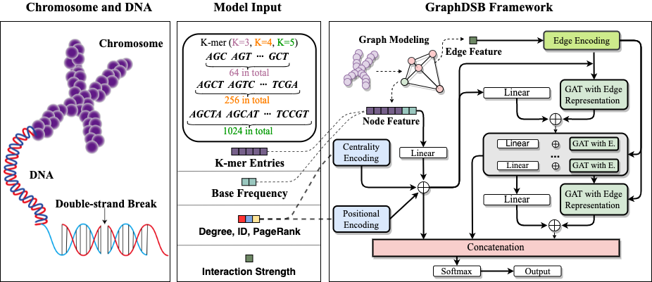
Figure 1: The overall architecture of the proposed GraphDSB, including the illustration of double-strand DNA break and K-mer entries, graph modeling of chromosomes, the composition of node features, and the network architecture. The $\bigoplus$ represents the addition operation between matrices.

The Proposed Framework

In this section, we introduce the proposed GraphDSB in detail, which includes graph modeling of chromosomes, a GNN framework based on self-attention (Veličković et al. 2017) with edge representation and JK-Network (Xu et al. 2018b), the centrality encoding which includes degree and PageRank (Page et al. 1999), and the positional encoding which uses node IDs. The overall framework is shown in the right part of Figure 1.

Graph Modeling of Chromosomes

First, in order to use the information provided by chromosome structure and DNA shape, we model the chromosome as a graph structure $G=(V,E)$, in which node $v_{i}\in V$ represents a 5-kb genome bin. The label of each node is represented by $y_{i}\in\{0,1\}$, where $1$ means a double-strand break has occurred, and $0$ means normal. The edges $E$ reflect the interaction strength between these bins, i.e., the contact frequency of corresponding entry in Hi-C contact map we collected, which reflects the chromosome structural information. The intention of our model is to fit the mapping relationship between chromosome structure, DNA sequencing results and DSBs, so we define DSBs prediction as a node-level binary classification problem.

In order to save the computing resources, we extract K-mer entries as shown in Figure 1, where K-mer represents the DNA sequence with length K, and K-mer entries is the frequency of these sequences, which are widely used in the analysis of genome sequence (Chor et al. 2009), and calculate their frequency distribution to replace the one-hot coding of AGCT sequence (Kurtz et al. 2008). Furthermore, we introduce base frequency, which refers to the frequency of each bases, i.e., $A,G,C,T$, in the whole genome bin to enrich node features.

The GraphDSB Framework

After modeling the chromosome into a graph, we then design a GNN architecture to aggregate structural information of the graph. Let the feature vector of node $v_{i}$ be $\bm{x}_{i}$, for the representation of nodes, modern GNN framework is generally expressed as two steps: aggregation of neighbor messages and update of representation. Specifically, denote $\bm{h}_{i}^{(l)}$ as the representaiton of $v_{i}$ in the $l$-th layer and define $\bm{h}_{i}^{(0)}=\bm{x}_{i}$. The computation of neighborhood aggregation and update in the $l$-th layer is in the following:

$$\bm{m}_{i}^{(l)}=\text{AGG}^{(l)}\left(\left\{\bm{h}_{j}^{(l-1)}:j\in N(v_{i})\right\}\right),$$ (1)

$$\bm{h}_{i}^{(l)}=\text{UPDATE}^{(l)}\left(\bm{h}_{i}^{(l-1)},\bm{m}_{i}^{(l)}\right)\text{,}$$

where $\bm{m}_{i}^{(l)}$ represents the message aggregated from the neighbors of $v_{i}$ in the $l$-th layer, and $N(v_{i})$ is the set of first-order neighbors of $v_{i}$.

Graph attention with edge representation. Tbe original GAT (Veličković et al. 2017) does not introduce edge features into the calculation of attention coefficient, which is not sufficient to predict DSBs, since edge features contain important structural information of chromosomes. Therefore, we introduce edge features as follows:

$$\bm{\alpha}_{ij}=\frac{\text{exp}(\text{LeakyReLU}\big{(}\bm{a}^{T}[\bm{W}_{N}\bm{h}_{i}||\bm{W}_{N}\bm{h}_{j}||\bm{W}_{E}\bm{h}_{(i,j)}])\big{)}}{\sum_{k\in N(v_{i})}\text{exp}\big{(}\text{LeakyReLU}(\bm{a}^{T}[\bm{W}_{N}\bm{h}_{i}||\bm{W}_{N}\bm{h}_{k}||\bm{W}_{E}\bm{h}_{(i,k)}])\big{)}},$$ (2)

where $\bm{a}$ is a learnable weight vector, $\bm{W}_{N}$ and $\bm{W}_{E}$ denote two trainable weight matrix, respectively, and $||$ dentoes the concatenation operation. The edge feature $\bm{h}_{(i,j)}$ is obtained from the interaction strength $\bm{e}_{(i,j)}$ between two genome bins through a linear layer, which is defined as edge encoding. The purpose of edge encoding is to keep the edge feature and the node feature dimension consistent.

To further improve the expression ability of the model, we introduce the JK-Network architecture here, as shown in Figure 1. Because the final representation of nodes can be adaptively integrated the information of different layers, we can build a deeper network, so as to achieve better results in DSBs prediction, which is verified in our experiments.

Centrality encoding and positional encoding. Following Graphormer (Ying et al. 2021), we define a centrality encoding, which not only considers the degree of nodes, but also introduces PageRank. At the same time, considering the sequence of chromosome structure, we also introduce the positional encoding in Transformer (Vaswani et al. 2017) as a supplement to node features. Instead of the absolute position of words, we use the ID of the genome bin in the chromosome. Finally, we multiply them by different learnable matrices $\bm{W}_{deg}$, $\bm{W}_{pr}$ and $\bm{W}_{pos}$, to achieve the same dimension as the node features, and initialize the node representation in a summation way: $\bm{h}_{i}^{(0)}=\bm{x}_{i}+\bm{z}_{deg(v_{i})}+\bm{z}_{pr(v_{i})}+\bm{z}_{pos(v_{i})}$. By adding the centrality encoding and the positional encoding to the input, the model can capture both the semantic correlation and the node importance in the attention mechanism.

Since the task is to identify DSBs on chromosomes (node-level binary classification), we use cross-entropy as loss function.

Table 1: Statistics of the two datasets in the experiments.

Dataset	Avg. #Nodes	Avg. #Edges	Density(%)	Avg. P/N ratio
NHEK	24,123	1,126,839	0.489	6.26
K562	24,079	3,743,946	1.784	107.35

Experiments

Settings. We utilize the chromosomes in two human cells, respectively normal human epidermal keratinocytes (NHEK) and chronic myeloid leukemia cell line (K562) datasets. Among them, NHEK is a normal cell line, which is available from the epidermis, it is the major cell type in the epidermis (making up about 90%). K562 is a cancer cell line. Specifically, K562 cells were established as the first human immortalized myelogenous leukemia line. These two cell lines are often used as representatives for erythroleukemic normal and tumour cell respectively. Each of dataset contains 22 autosomes and X chromosome (we do not consider Y chromosome).

For each cell line, we gathered its (1) DSB dataset as well as (2) the Hi-C dataset which reflects the chromosome structural information. The DNA sequence is derived from the human reference genome. Because DSBs are more common in cancer cells, there is also a large gap in the positive-negative ratio (P/N ratio), as shown in Table 1.

For each dataset, we use 21 chromosomes as training, 1 as validation, and the remaining one as test, which is presented in the form of inductive learning. For the evaluation metric, we use Area Under Curve (AUC).

All models are implemented with Pytorch (version 1.7.0) (Paszke et al. 2019) on a GPU 2080Ti. In addition, in order to facilitate the implementation of various GNN variants, we use the popular GNN library: Deep Graph Library (DGL) (version 0.6.0) (Wang et al. 2019).

Table 2: Comparisons among different models in terms of average AUC with STDs. The best performance is in bold.

Method	NHEK	K562
LightGBM	$0.7507\pm 0.0299$	$0.7397\pm 0.0525$
MLP	$0.7623\pm 0.0291$	$0.7237\pm 0.0528$
GraphDSB	$\bm{0.7902\pm 0.0233}$	$0.7564\pm 0.0443$

Performance. In order to evaluate the contribution of the graph structure to the identification of DSBs, we select two effective models, LightGBM (Ke et al. 2017) and Multilyaer Perceptron (MLP), which do not depend on the graph structure, as the baselines. Our GNN model includes 1 input layer $(d=256)$, 4 GNN layers $(d=256)$, 1 full connection layer $(d=256\times 5)$ and 1 output layer$(d=1)$. The number of attention heads is set to 4. The MLP architecture is also five-layered, and the dimensions are consistent with GraphDSB. For LightGBM, we set reasonable parameter search field for each hyperparameter, and use Hyperopt (Bergstra et al. 2013) for automatic search, the number of serach iterations is setted to 100. For all NN method, We use Adam as the optimizer, the learning rate is set to 0.003, the exponential decay strategy is adopted and the rate is 0.99. The results are shown in Table 2.

In terms of average AUC, GraphDSB performs better than the other two methods that do not leverage on graph structure, which demonstrates the effectiveness of the graph modeling, i.e., chromosomes structures, on the prediction of DSBs.

Table 3: Ablation studies on the proposed GraphDSB.

Method	NHEK	K562
w/o JK	$0.7799\pm 0.0027$	$0.7451\pm 0.0044$
w/o E.R.	$0.7831\pm 0.0026$	$0.7472\pm 0.0045$
w/o C.E.	$0.7886\pm 0.0026$	$0.7428\pm 0.0045$
w/o P.E.	$0.7893\pm 0.0028$	$0.7531\pm 0.0047$
GCN	$0.7699\pm 0.0027$	$0.7353\pm 0.0046$
GAT	$0.7805\pm 0.0027$	$0.7448\pm 0.0044$
GIN	$0.7361\pm 0.0029$	$0.7361\pm 0.0046$
GraphDSB	$0.7902\pm 0.0023$	$0.7564\pm 0.0044$

Ablation study. The ablation study results are given in Table 3, including whether JK is included, whether interaction strength are introduced, whether centrality encoding and positional encoding is introduced, and the comparison with popular GNN variants, including GCN (Kipf and Welling 2016), GAT (Veličković et al. 2017) and GIN (Xu et al. 2018a). It can be seen that GAT performs better than the other two GNN methods, which proves the role of the attention mechanism from the side. While GraphDSB is better than these three GNN methods, it is also better than the four variants of GraphDSB, which verifies our original intention of designing the network framework, centrality encoding and positional encoding.

Explaining the results of GraphDSB. In order to analyze the contribution of node features and topologies to DSBs prediction, we introduce GNNExplainer, its core idea is to use the mutual information $MI(Y,(G_{s},X_{s}))$ between input substructures $G_{s}$ and sub features $X_{s}$ to measure the importance of node features and edges.

For all chromosomes, we first calculate the feature importance of all nodes and take the average value, and final count the TOP 20 feature numbers with the largest average value of importance. As shown in Figure 2(a), we found that 5-mer DNA sequence features(the index is between 321-1344) are more important than 3-mer or 4-mer DNA sequence features, suggesting the complex DNA sequence preference of DSBs.

Beyond important genomic features, we extract the importance of edges which provides a set of crucial chromatin interactions that are most influential to predict whether DSB occurs at a given genome site of interest. These interactions form a functional module that corresponds to a series of genome regions that have pair-wise interactions nearby the prediction site. We referred to this module as DSB associated chromatin interaction module (DaCIM) for that prediction site. We limit the edge importance calculation to 2-hop neighbor, and found a group of motifs: recurring and significant patterns of chromatin interactions in DaCIM. The most frequent motifs tend to have a mode termed ’forward chain’ and ’binary-parallel’ Figure 2(b). These motifs suggests DaCIM may contain the universal build block at interaction level for chromatin organization. Similar discoveries have also been made in (Falk, Lukasova, and Kozubek 2010), which discussed the role of higher-order chromatin structure in DSB induction and repair.

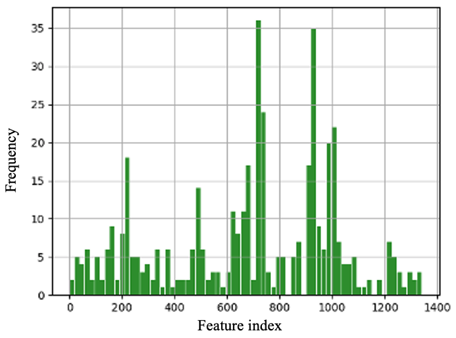
(a) Node features importance

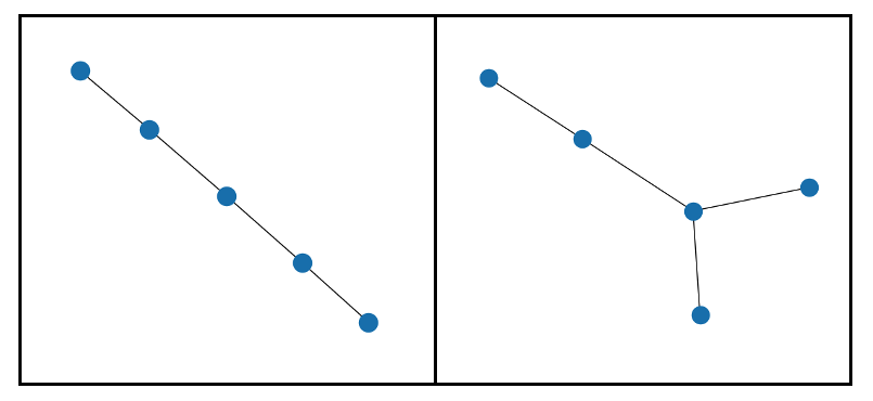
(b) The most frequent motifs

Figure 2: The results of GNNExplainer application on GraphDSB. (a) The distribution of the importance of the node feature. The TOP20 feature ID is counted and recorded on each chromosome. The vertical axis indicates the frequency of the feature ID in the TOP20. In order to facilitate the display, the 1344-dimensional features are grouped into 70 bins. (b) The most frequent motifs, the left is the ’forward chain’ and the right is the ’binary-parallel’.

Related Work

DSB is generally detected based on high-throughput experiments. For example, (Crosetto et al. 2013) proposed a method of direct in situ break labeling, streptavidin enrichment and next-generation sequencing to draw DSBs with nucleotide resolution. There are other methods, such as (Biernacka et al. 2018; Keimling et al. 2008). Although high-throughput technology allows genome-wide mapping of DSBs with high resolution, high cost and high technical difficulty are still unavoidable problems. Recently, more and more studies have focused on low-cost, high-efficiency DSBs prediciton. (Mourad et al. 2018) demonstrate, that endogenous DSBs can be computationally predicted using the epigenomic and chromatin context, and it used Random Forest as a model for predicting DSBs. However, compared to the proposed GraphDSB, this method does not use the structural information of chromosomes when predicting DSBs, and some studies have shown that the shape of DNA has a certain correlation with DSBs (Taverna et al. 2007; Zhou and Troyanskaya 2015; Mathelier et al. 2016).

Recent years have witnessed the effectiveness of graph neural network on graph-structured data. Representative GNNs, including graph convolutional network (GCN) (Kipf and Welling 2016), GraphSAGE (Hamilton, Ying, and Leskovec 2017), graph attention network (GAT) (Veličković et al. 2017), graph isomorphsim network (GIN) (Xu et al. 2018a), have been widely used for different graph-based tasks. For GNN, graph structured inputs offer representational flexibility, which can naturally model proteins, moleclues and so on. Therefore, GNN has also made significant development in biology and genomics in recent years (Ingraham et al. 2019; Fout 2017; Nguyen et al. 2021; Wang et al. 2021). However, to the best of our knowledge, in this work, we make the first attempt to explore the ability of GNN on the prediction of DSBs by modeling the chromosome structure.

Conclusion

In this work, we explore the GraphDSB to DSBs prediction, which uses DNA sequence features and chromosome structure information as input. GraphDSB performes better than other GNN variants on the two datasets of the normal cell line NHEK and the cancer cell line K562, which verifies the effectiveness of the proposed framework and several structural encodings methods. We also used GNNExplainer to prove the effectiveness of 5-mer DNA sequence features and found two important interaction modes for DSBs prediction. In the future, we will explore the neural architecture search method and apply the existing work to the field of biomedicine(Zhang, Wang, and Zhu 2021; Huan, Quanming, and Weiwei 2021; Wei et al. 2021; Wei, Zhao, and He 2021).

References

- Battaglia et al. (2018) Battaglia, P. W.; Hamrick, J. B.; Bapst, V.; Sanchez-Gonzalez, A.; Zambaldi, V.; Malinowski, M.; Tacchetti, A.; Raposo, D.; Santoro, A.; Faulkner, R.; et al. 2018. Relational inductive biases, deep learning, and graph networks. arXiv preprint arXiv:1806.01261.
- Bergstra et al. (2013) Bergstra, J.; Yamins, D.; Cox, D. D.; et al. 2013. Hyperopt: A python library for optimizing the hyperparameters of machine learning algorithms. In Proceedings of the 12th Python in science conference, volume 13, 20. Citeseer.
- Biernacka et al. (2018) Biernacka, A.; Zhu, Y.; Skrzypczak, M.; Forey, R.; Pardo, B.; Grzelak, M.; Nde, J.; Mitra, A.; Kudlicki, A.; Crosetto, N.; et al. 2018. i-BLESS is an ultra-sensitive method for detection of DNA double-strand breaks. Communications biology, 1(1): 1–9.
- Chereda et al. (2019) Chereda, H.; Bleckmann, A.; Kramer, F.; Leha, A.; and Beissbarth, T. 2019. Utilizing Molecular Network Information via Graph Convolutional Neural Networks to Predict Metastatic Event in Breast Cancer. In GMDS, 181–186.
- Chor et al. (2009) Chor, B.; Horn, D.; Goldman, N.; Levy, Y.; and Massingham, T. 2009. Genomic DNA k-mer spectra: models and modalities. Genome biology, 10(10): 1–10.
- Crosetto et al. (2013) Crosetto, N.; Mitra, A.; Silva, M. J.; Bienko, M.; Dojer, N.; Wang, Q.; Karaca, E.; Chiarle, R.; Skrzypczak, M.; Ginalski, K.; et al. 2013. Nucleotide-resolution DNA double-strand break mapping by next-generation sequencing. Nature methods, 10(4): 361–365.
- Falk, Lukasova, and Kozubek (2010) Falk, M.; Lukasova, E.; and Kozubek, S. 2010. Higher-order chromatin structure in DSB induction, repair and misrepair. Mutation Research/Reviews in Mutation Research, 704(1-3): 88–100.
- Fout (2017) Fout, A. M. 2017. Protein interface prediction using graph convolutional networks. Ph.D. thesis, Colorado State University.
- Hamilton, Ying, and Leskovec (2017) Hamilton, W. L.; Ying, R.; and Leskovec, J. 2017. Inductive representation learning on large graphs. In Proceedings of the 31st International Conference on Neural Information Processing Systems, 1025–1035.
- Huan, Quanming, and Weiwei (2021) Huan, Z.; Quanming, Y.; and Weiwei, T. 2021. Search to aggregate neighborhood for graph neural network. In 2021 IEEE 37th International Conference on Data Engineering (ICDE), 552–563. IEEE.
- Ingraham et al. (2019) Ingraham, J.; Garg, V. K.; Barzilay, R.; and Jaakkola, T. 2019. Generative models for graph-based protein design.
- Ke et al. (2017) Ke, G.; Meng, Q.; Finley, T.; Wang, T.; Chen, W.; Ma, W.; Ye, Q.; and Liu, T.-Y. 2017. Lightgbm: A highly efficient gradient boosting decision tree. Advances in neural information processing systems, 30: 3146–3154.
- Keimling et al. (2008) Keimling, M.; Kaur, J.; Bagadi, S. A. R.; Kreienberg, R.; Wiesmüller, L.; and Ralhan, R. 2008. A sensitive test for the detection of specific DSB repair defects in primary cells from breast cancer specimens. International journal of cancer, 123(3): 730–736.
- Kipf and Welling (2016) Kipf, T. N.; and Welling, M. 2016. Semi-supervised classification with graph convolutional networks. arXiv preprint arXiv:1609.02907.
- Kurtz et al. (2008) Kurtz, S.; Narechania, A.; Stein, J. C.; and Ware, D. 2008. A new method to compute K-mer frequencies and its application to annotate large repetitive plant genomes. BMC genomics, 9(1): 1–18.
- Lensing et al. (2016) Lensing, S. V.; Marsico, G.; Hänsel-Hertsch, R.; Lam, E. Y.; Tannahill, D.; and Balasubramanian, S. 2016. DSBCapture: in situ capture and sequencing of DNA breaks. Nature methods, 13(10): 855–857.
- Mathelier et al. (2016) Mathelier, A.; Xin, B.; Chiu, T.-P.; Yang, L.; Rohs, R.; and Wasserman, W. W. 2016. DNA shape features improve transcription factor binding site predictions in vivo. Cell systems, 3(3): 278–286.
- McKinnon and Caldecott (2007) McKinnon, P. J.; and Caldecott, K. W. 2007. DNA strand break repair and human genetic disease. Annu. Rev. Genomics Hum. Genet., 8: 37–55.
- Mehta and Haber (2014) Mehta, A.; and Haber, J. E. 2014. Sources of DNA double-strand breaks and models of recombinational DNA repair. Cold Spring Harbor perspectives in biology, 6(9): a016428.
- Mourad et al. (2018) Mourad, R.; Ginalski, K.; Legube, G.; and Cuvier, O. 2018. Predicting double-strand DNA breaks using epigenome marks or DNA at kilobase resolution. Genome biology, 19(1): 1–14.
- Nguyen et al. (2021) Nguyen, T.; Le, H.; Quinn, T. P.; Nguyen, T.; Le, T. D.; and Venkatesh, S. 2021. GraphDTA: Predicting drug–target binding affinity with graph neural networks. Bioinformatics, 37(8): 1140–1147.
- Page et al. (1999) Page, L.; Brin, S.; Motwani, R.; and Winograd, T. 1999. The PageRank citation ranking: Bringing order to the web. Technical report, Stanford InfoLab.
- Paszke et al. (2019) Paszke, A.; Gross, S.; Massa, F.; Lerer, A.; Bradbury, J.; Chanan, G.; Killeen, T.; Lin, Z.; Gimelshein, N.; Antiga, L.; et al. 2019. Pytorch: An imperative style, high-performance deep learning library. Advances in neural information processing systems, 32: 8026–8037.
- Rhee, Seo, and Kim (2017) Rhee, S.; Seo, S.; and Kim, S. 2017. Hybrid approach of relation network and localized graph convolutional filtering for breast cancer subtype classification. arXiv preprint arXiv:1711.05859.
- Taverna et al. (2007) Taverna, S. D.; Li, H.; Ruthenburg, A. J.; Allis, C. D.; and Patel, D. J. 2007. How chromatin-binding modules interpret histone modifications: lessons from professional pocket pickers. Nature structural & molecular biology, 14(11): 1025–1040.
- Vaswani et al. (2017) Vaswani, A.; Shazeer, N.; Parmar, N.; Uszkoreit, J.; Jones, L.; Gomez, A. N.; Kaiser, Ł.; and Polosukhin, I. 2017. Attention is all you need. In Advances in neural information processing systems, 5998–6008.
- Veličković et al. (2017) Veličković, P.; Cucurull, G.; Casanova, A.; Romero, A.; Lio, P.; and Bengio, Y. 2017. Graph attention networks. arXiv preprint arXiv:1710.10903.
- Wang et al. (2019) Wang, M.; Yu, L.; Zheng, D.; Gan, Q.; Gai, Y.; Ye, Z.; Li, M.; Zhou, J.; Huang, Q.; Ma, C.; et al. 2019. Deep Graph Library: Towards Efficient and Scalable Deep Learning on Graphs.
- Wang et al. (2021) Wang, Y.; Abuduweili, A.; Yao, Q.; and Dou, D. 2021. Property-aware relation networks for few-shot molecular property prediction. Advances in Neural Information Processing Systems, 34.
- Wei, Zhao, and He (2021) Wei, L.; Zhao, H.; and He, Z. 2021. Designing the Topology of Graph Neural Networks: A Novel Feature Fusion Perspective. arXiv:2112.14531.
- Wei et al. (2021) Wei, L.; Zhao, H.; Yao, Q.; and He, Z. 2021. Pooling architecture search for graph classification. In Proceedings of the 30th ACM International Conference on Information & Knowledge Management, 2091–2100.
- Wu et al. (2020) Wu, X.; Lan, W.; Chen, Q.; Dong, Y.; Liu, J.; and Peng, W. 2020. Inferring lncRNA-disease associations based on graph autoencoder matrix completion. Computational biology and chemistry, 87: 107282.
- Xu et al. (2018a) Xu, K.; Hu, W.; Leskovec, J.; and Jegelka, S. 2018a. How powerful are graph neural networks? arXiv preprint arXiv:1810.00826.
- Xu et al. (2018b) Xu, K.; Li, C.; Tian, Y.; Sonobe, T.; Kawarabayashi, K.-i.; and Jegelka, S. 2018b. Representation learning on graphs with jumping knowledge networks. In International Conference on Machine Learning, 5453–5462. PMLR.
- Ying et al. (2021) Ying, C.; Cai, T.; Luo, S.; Zheng, S.; Ke, G.; He, D.; Shen, Y.; and Liu, T.-Y. 2021. Do Transformers Really Perform Bad for Graph Representation? arXiv preprint arXiv:2106.05234.
- Ying et al. (2019) Ying, R.; Bourgeois, D.; You, J.; Zitnik, M.; and Leskovec, J. 2019. Gnnexplainer: Generating explanations for graph neural networks. Advances in neural information processing systems, 32: 9240.
- Zhang et al. (2019) Zhang, H.; Liang, Y.; Peng, C.; Han, S.; Du, W.; and Li, Y. 2019. Predicting lncRNA-disease associations using network topological similarity based on deep mining heterogeneous networks. Mathematical biosciences, 315: 108229.
- Zhang, Wang, and Zhu (2021) Zhang, Z.; Wang, X.; and Zhu, W. 2021. Automated Machine Learning on Graphs: A Survey. arXiv preprint arXiv:2103.00742.
- Zhao et al. (2020) Zhao, T.; Hu, Y.; Peng, J.; and Cheng, L. 2020. DeepLGP: a novel deep learning method for prioritizing lncRNA target genes. Bioinformatics, 36(16): 4466–4472.
- Zhou and Troyanskaya (2015) Zhou, J.; and Troyanskaya, O. G. 2015. Predicting effects of noncoding variants with deep learning–based sequence model. Nature methods, 12(10): 931–934.