Approximation Algorithms for Maximum Matchings in Geometric Intersection Graphs

Abstract

We present a $(1-{\varepsilon})$-approximation algorithms for maximum cardinality matchings in disk intersection graphs – all with near linear running time. We also present an estimation algorithm that returns $(1\pm{\varepsilon})$-approximation to the size of such matchings – this algorithm runs in linear time for unit disks, and $O(n\log n)$ for general disks (as long as the density is relatively small).

1 Introduction

Geometric intersection graphs

Given a set of $n$ objects $\mathsf{U}$, its intersection graph, $\mathcal{I}_{\mathsf{U}}$, is the graph where the vertices correspond to objects in $\mathsf{U}$ and there is an edge between two vertices if their corresponding objects intersect. Such graphs can be dense (i.e., have $\Theta(n^{2})$ edges), but they have a linear size representation. It is natural to ask if one can solve problems on such graphs more efficiently than explicitly represented graphs.

Maximum matchings

Computing maximum cardinality matchings is one of the classical problems on graphs (surprisingly, the algorithm to solve the bipartite case goes back to work by Jacobi in the mid 19th century). The fastest combinatorial algorithm (ignoring polylog factors) seems to be the work by Gabow and Tarjan [GT91], running in $O(m\sqrt{n})$ time where $m$ is the number of edges in the graph. Harvey [Har09] and Mucha and Sankowski [MS04] provided algorithms based on algebraic approach that runs in $O(n^{\omega})$ time, where $O(n^{\omega})$ is the fastest time known for multiplying two $n\times n$ matrices. Currently, the fastest known algorithm for matrix multiplication has $\omega\approx 2.3728596$, but it is far from being practical.

Matchings for planar graphs and disk intersection graphs

Mucha and Sankowski [MS06] adapted their algebraic technique for planar graphs (specifically using separators), getting running time $O(n^{\omega/2})\approx O(n^{1.17})$. Yuster and Zwick [YZ07] adapted this algorithm for graphs with excluded minors.

Maximum matchings in geometric intersection graphs

Bonnet et al. [BCM20] studied the problem for geometric intersection graphs. For simplicity of exposition, we describe their results in the context of disk intersection graphs. Given a set $n$ disks with maximum density $\rho$ (i.e., roughly the maximum number of disks covering a point in the plane), they presented an algorithm for computing maximum matchings with running time $O(\rho^{3\omega/2}n^{\omega/2})\approx O(\rho^{3.5}n^{1.17})$. This compares favorably with the naive algorithm of just plugging such graphs into the algorithm of Gabow and Tarjan, which yields running time $O(m\sqrt{n})=O(\rho n^{3/2})$. If the ratio between the smallest disk and largest disk is at most $\Phi$, they presented an algorithm with running time $O(\Phi^{12\omega}n^{\omega/2})$. Note that the running time of all these algorithms is super linear in $n$.

Approximate maximum matchings

It is well known that it is enough to augment along paths of length up to $O(1/{\varepsilon})$ if one wants $(1-{\varepsilon})$-approximate matchings. For bipartite graphs this implies that one need to run $O(1/{\varepsilon})$ rounds of paths finding stage of the bipartite matching algorithm of Hopcroft and Karp [HK73]. Since such a round takes $O(m)$ time, this readily leads to an $(1-{\varepsilon})$-approximate bipartite matching algorithm in this case. The non-bipartite case is significantly more complicated, and the weighted case is even more difficult. Nevertheless, Duan and Pettie [DP14] presented an algorithm with running time $O(m{\varepsilon}^{-1}\log{{\varepsilon}^{-1}})$ which provides $(1-{\varepsilon})$-approximation to the maximum weight matching in non-bipartite graph.

Density and approximate matchings

For a set of objects $\mathsf{U}$ in $\mathbb{R}^{d}$, the density of an object is the number of bigger objects in the set intersecting it. The density of the set of objects is the maximum density of the objects. The density is denoted by $\rho$, and the premise is that for real world inputs it would be small. The intersection graph of such objects when $\rho$ is a constant are known as low density graphs, have some nice properties, such as having separators. See [HQ17] and references therein. In particular, for a set of fat objects, the density and the maximum depth (i.e., the maximum number of object covering any point) are roughly the same. It is well known that low density graphs are sparse and have $O(\rho n)$ edges, where $n$ is the number of objects in the set. Since one can compute the intersection graph in $O(n\log n+\rho n)$ time, and plug it into the algorithm of Duan and Pettie [DP14], it follows that an approximation algorithm with running time $O\bigl{(}n\log n+(\rho n/{\varepsilon})\log(1/{\varepsilon})\bigr{)}$. See Section 4.2 for details. Thus, the challenge is to get better running times than this baseline.

1.1 Our results

Our purpose here is to develop near linear time algorithms for approximate matchings for the unit disk graph and the general disk graph cases. Our results are summarized in Table 1.1. Note, in this paper, we assume the input to our algorithms to be a set of disks.

1. Unit disk graph.

   1. Greedy matching. We show in Section 3.1 a linear time algorithm for the case of unit disks graph – this readily provides a $1/2$-approximation to the maximum matching. The algorithm uses a simple grid to “capture’ intersections, and then use the locality of the grid to find intersection with the remaining set of disks.

   2. $(1-{\varepsilon})$-approximation. In Section 3.2 we show how to get a $(1-{\varepsilon})$-approximation. The running time can be bounded by $O\bigl{(}(n/{\varepsilon}^{2})\log(1/{\varepsilon})\bigr{)}$. If the diameter of union of disks is at most $\Delta$, then the running time is $O\bigl{(}n+(\Delta^{2}/{\varepsilon}^{2})\log(1/{\varepsilon})\bigr{)}$.

   3. $(1-{\varepsilon})$-estimation. Surprisingly, one can do even better – we show in Section 3.3 how to use importance sampling to get $(1\pm{\varepsilon})$-approximation (in expectation) to the size of the maximum matching in time $O(n+\textrm{poly}(\log n,1/{\varepsilon}))$.

2. Disk graph. The general disk graph case is more challenging.

   1. Greedy matching. The greedy matching algorithm can be implemented in $O(n\log n)$ time using sweeping, see Lemma 4.1 (this algorithm works for any nicely behaved shapes).

   2. Approximate bipartite case. Here, we are given two sets of disks, and consider only intersections across the sets as edges. This case can be solved using range searching data-structures as was done by Efrat et al. [EIK01] – they showed how to implement a round of the bipartite matching algorithm of Hopcroft and Karp [HK73] using $O(n)$ queries. It is folklore that running $O(1/{\varepsilon})$ rounds of this algorithm leads to a $(1-{\varepsilon})$-approximation algorithm. Coupling this with the data-structure of Kaplan et al. [KMR+20] readily leads to a near linear approximation algorithm in this case, see Section 4.3.

   3. $(1-{\varepsilon})$-approximation algorithm. Surprisingly, approximate general matchings can be reduced to bipartite matchings via random coloring. Specifically, one can compute $(1-{\varepsilon})$-approximate matchings using $2^{O(1/{\varepsilon})}\log n$ invocations of approximate bipartite matchings algorithm mentioned above. This rather neat idea is due to Lotker et al. [LPP15] who used in the context of parallel matching algorithms. This leads to a near linear time algorithm for $(1-{\varepsilon})$-approximate matchings for disk intersection graphs, see Section 4.4 for details. The running time of the resulting algorithm is $2^{O(1/{\varepsilon})}n\log^{O(1)}n$.

      We emphasize that this algorithm assumes nothing about the density of the input disks.

   4. $(1-{\varepsilon})$-estimation. One can get an $O(n\log n)$ time estimation algorithm in this case, but one needs to assume that the input disks have “small” density $\rho$. Specifically, one computes a separator hierarchy and then use importance sampling on the patches, as to estimate the sampling size. The details require some care, see Section 4.6. The resulting algorithm has running time $O(n\log n)$ if the density is $o(n^{1/9})$.

3. General shapes. Somewhat surprisingly, almost all our results extends in a verbatim fashion to intersection graphs of general shapes. We need some standard assumptions about the shapes:

   1. the boundary of any pair of shapes intersects only a constant number of times,

   2. these intersections can be computed in constant time,

   3. one can compute the $x$-extreme and $y$-extreme points in a shape in constant time,

   4. one can decide in constant time if a point is inside a shape, and

   5. the boundary of a shape intersects any line a constant number of times, and they can be computed in constant time.

   For fat shapes of similar size, we also assume the diameters of all the shapes are the same up to a constant factor, and any object $o$ contains a disk of radius $\Omega(\text{diam}\left({o}\right))$.

   Since the modification needed to make the algorithms work for the more general cases are straightforward, we describe the algorithms for disks.

The full version of the paper is available on the [HY22].

Shape	Quality	Running time	Ref	Comment
Unit disks Fat shapes of similar size	$1/2$	$O(n)$	Lemma 3.1	Greedy
	$1-{\varepsilon}$	$O\bigl{(}\frac{n}{{\varepsilon}}\log\frac{1}{{\varepsilon}}\bigr{)}\Bigr{.}$	Lemma 3.3
		$O\bigl{(}n+(\Delta^{2}/{{\varepsilon}^{2}})\log\frac{1}{{\varepsilon}}\bigr{)}\Bigr{.}$	Remark 3.4	$\Delta$ = Diam. disks
	$1\pm{\varepsilon}$	$O(n+{\varepsilon}^{-6}\log^{2}n)\Bigr{.}$	Theorem 3.5	Estimation
Unit disks	$1-{\varepsilon}$	$O\bigl{(}\frac{n}{{\varepsilon}}\log\frac{1}{{\varepsilon}}\bigr{)}\Bigr{.}$	Lemma 3.3	Approximate
Disks	$1-{\varepsilon}$	$O\bigl{(}(n/{\varepsilon})\log^{11}n\bigr{)}\Bigr{.}$	Lemma 4.4 ($\star$)	Bipartite
	$1-{\varepsilon}$	$O(2^{O(1/{\varepsilon})}n\log^{12}n)\Bigr{.}$	Theorem 4.6 ($\star$)	General
Shapes	$1/2$	$O(n\log n)$	Lemma 4.1	Greedy
	$1-{\varepsilon}$	$O(n\log n+\frac{m}{{\varepsilon}}\log\frac{1}{{\varepsilon}})\Bigr{.}$	Lemma 4.2	$m:$ # edges
	$1-{\varepsilon}$	$O(n\log n+\frac{n\rho}{{\varepsilon}}\log\frac{1}{{\varepsilon}})\Bigr{.}$	Lemma 4.3	$\rho$: Density
	Exact	$O(n\log n)$	Lemma 4.8	Matching size $O(n^{1/8})\Bigr{.}$
	$1\pm{\varepsilon}$	$O(n\log n+\rho^{9}{\varepsilon}^{-19}\log^{2}n)\Bigr{.}$	Theorem 4.13	Estimation

Table 1.1: Results. The ($\star$) indicates the result works only for disks.

2 Preliminaries

2.1 Notations

For a graph $G$, let $\mathcal{M}^{\star}_{G}$ denote the maximum cardinality matching in $G$. Its size is denoted by $\mathcalb{m}^{\star}=\mathcalb{m}^{\star}\left({G}\right)=\left|{\mathcal{M}^{\star}_{G}}\right|$. For a graph $G=(\mathsf{V},\mathsf{E})$, and a set $X\subseteq\mathsf{V}$ the induced subgraph of $G$ over $X$ is $G_{|{X}}=\bigl{(}X,\left\{uv\in\mathsf{E}\;\middle|\;u,v\in X\right\}\bigr{)}$. For a set $Z$, let $G-Z$ denote the graph resulting from $G$ after deleting from it all the vertices of $Z$. Formally, $G-Z$ is the graph $G_{|{\mathsf{V}\setminus Z}}$.

Definition 2.1.

For a set of objects $\mathsf{U}$, the intersection graph of $\mathsf{U}$, denoted by $\mathcal{I}_{\mathsf{U}}$, is the graph having $\mathsf{U}$ as its set of vertices, and there is an edge between two objects $o,g\in\mathsf{U}$ if they intersect. Formally,

$$\mathcal{I}_{\mathsf{U}}=\left({\bigl{.}\mathsf{U},\left\{\bigl{.}og\;\middle|\;o,g\in\mathsf{U}\text{ and }o\cap g\neq\emptyset\right\}}\right).$$

For a point $p\in\mathbb{R}^{2}$, and a set of disks $\mathcal{D}$, let

$$\mathcal{D}\sqcap p=\left\{\Circle\in\mathcal{D}\;\middle|\;p\in\Circle\right\}$$

be the set of disks of $\mathcal{D}$ that contain $p$. Note, that the intersection graph $\mathcal{I}_{p}=\mathcal{I}_{\mathcal{D}\cap p}$ is a clique.

Definition 2.2.

Consider a set of disks $\mathcal{D}$. A set $\mathcal{D}^{\prime}\subseteq\mathcal{D}$ is an independent set (or simply independent) if no pair of disks of $\mathcal{D}^{\prime}$ intersects.

2.2 Low density and separators

The following is standard by now, see Har-Peled and Quanrud [HQ17] and references therein.

Definition 2.3.

A set of objects $\mathsf{U}$ in $\mathbb{R}^{d}$ (not necessarily convex or connected) has density $\rho$ if any object $o$ (not necessarily in $\mathsf{U}$) intersects at most $\rho$ objects in $\mathsf{U}$ with diameter equal or larger than the diameter of $o$. The minimum such quantity is denoted by $\mathop{\mathrm{density}}\left({\mathsf{U}}\right)$. A graph that can be realized as the intersection graph of a set of objects $\mathsf{U}$ in $\mathbb{R}^{d}$ with density $\rho$ is $\rho$-dense. The set $\mathsf{U}$ is low density if $\rho=O(1)$.

Definition 2.4.

Let $G=(\mathsf{V},\mathsf{E})$ be an undirected graph. Two sets $X,Y\subseteq\mathsf{V}$ are separate in $G$ if

1. $X$ and $Y$ are disjoint, and

2. there is no edge between the vertices of $X$ and the vertices of $Y$ in $G$.

For a constant $\zeta\in(0,1)$, a set $Z\subseteq\mathsf{V}$ is a $\zeta$-separator for a set $U\subseteq\mathsf{V}$, if $U\setminus Z$ can be partitioned into two separate sets $X$ and $Y$, with $\left|{X}\right|\leq\zeta\left|{U}\right|$ and $\left|{Y}\right|\leq\zeta\left|{U}\right|.$

Lemma 2.5 ([HQ17]).

Let $\mathsf{U}$ be a set of $n$ objects in $\mathbb{R}^{d}$ with density $\rho$. One can compute, in expected linear time, a sphere ${\mathbb{{S}}}$ that intersects in expectation $\tau=O\left({\rho+\rho^{1/d}n^{1-1/d}}\right)$ objects of $\mathsf{U}$. The sphere is computed by picking uniformly its radius from some range of the form $[\alpha,2\alpha]$. Furthermore, the total number of objects of $\mathsf{U}$ strictly inside/outside ${\mathbb{{S}}}$ is at most $\zeta n$, where $\zeta$ is a constant that depends only on $d$. Namely, the intersection graph $\mathcal{I}_{\mathsf{U}}$ has a separator of size $\tau$ formed by all the objects of $\mathsf{U}$ intersecting ${\mathbb{{S}}}$.

2.3 Importance sampling

Importance sampling is a standard technique for estimating a sum of terms. Assume that for each term in the summation, one can quickly get a coarse estimate of its value. Furthermore, assume that better estimates are possible but expensive. Importance sampling shows how to sample terms in the summation, then acquire a better estimate only for the sampled terms, to get a good estimate for the full summation. In particular, the number of samples is bounded independently of the original number of terms, depending instead on the coarseness of the initial estimates, the probability of success, and the quality of the final output estimate.

Lemma 2.6 ([BHR+20]).

Let $(\mathcal{H}_{1},w_{1},e_{1}),\ldots,(\mathcal{H}_{r},w_{r},e_{r})$ be given, where $\mathcal{H}_{i}$’s are some structures, and $w_{i}$ and $e_{i}$ are numbers, for $i=1,\ldots,r$. Every structure $\mathcal{H}_{i}$ has an associated weight $\overline{\mathsf{w}}\left({\mathcal{H}_{i}}\right)\geq 0$ (the exact value of $\overline{\mathsf{w}}\left({\mathcal{H}_{i}}\right)$ is not given to us). In addition, let $\xi>0$, $\gamma$, $b$, and $M$ be parameters, such that:

1. $\forall i\quad w_{i},e_{i}\geq 1$,

2. $\forall i\quad e_{i}/b\leq\overline{\mathsf{w}}\left({\mathcal{H}_{i}}\right)\leq e_{i}b$, and

3. $\Gamma=\sum_{i}w_{i}\cdot\overline{\mathsf{w}}\left({\mathcal{H}_{i}}\right)\leq M$.

Then, one can compute a new sequence of triples $(\mathcal{H}_{1}^{\prime},w_{1}^{\prime},e_{1}^{\prime}),\ldots,(\mathcal{H}_{t}^{\prime},w_{t}^{\prime},e_{t}^{\prime})$, that also complies with the above conditions, such that the estimate $Y=\sum_{i=1}^{t}w_{i}^{\prime}\overline{\mathsf{w}}\left({\mathcal{H}_{i}^{\prime}}\right)$ is a multiplicative $(1\pm\xi)$-approximation to $\Gamma$, with probability $\geq 1-\gamma$. The running time of the algorithm is $O(r)$, and size of the output sequence is $t=O\left({b^{4}\xi^{-2}(\log\log M+\log\gamma^{-1})\log M}\right).$

Remark 2.7.

The algorithm of Lemma 2.6 does not use the entities $\mathcal{H}_{i}$ directly at all. In particular, the $\mathcal{H}_{i}^{\prime}$s are just (reweighed) copies of some original structures. The only thing that the above lemma uses is the estimates $e_{1},\ldots,e_{r}$ and the weights $w_{1},\ldots,w_{r}$.

(B) We are going to use Lemma 2.6, with $\xi=O({\varepsilon})$, $\gamma=1/n^{O(1)}$, $b=2$, and $M=n$. As such, the size of the output list is $L_{\mathrm{len}}=O({\varepsilon}^{-2}\log^{2}n)$

2.4 Background on matchings

For a graph $G$, a matching is a set $\mathcal{C}\subseteq E\left({G}\right)$ of edges, such that no pair of them not share an endpoint. A matching that has the largest cardinality possible for a graph $G$, is a maximum matching. Given a graph $G$ and a matching $\mathcal{C}$ on $G$, an alternating path is a path with edges that alternate between matched edges (i.e., edges that are in $\mathcal{C}$) and unmatched edges (i.e., edges in $E\left({G}\right)\setminus\mathcal{C}$). If both endpoints of an alternating path are unmatched (i.e., free), then it is an augmenting path. In the following, let $\mathcal{M}^{\star}$ denote a maximum cardinality matching in $G$, and let $\mathcalb{m}^{\star}=\mathcalb{m}^{\star}\left({G}\right)=|\mathcal{M}^{\star}|$ denote its size. For $\beta\in[0,1]$, a matching $\mathcal{B}\subseteq E\left({G}\right)$ is an $\beta$-matching (or $\beta$-approximate matching) if $\left|{\mathcal{B}}\right|\geq\beta\mathcalb{m}^{\star}$. The set of vertices covered by the matching $\mathcal{B}$ is denoted by $\mathsf{V}\left({\mathcal{B}}\right)=\displaystyle\bigcup_{uv\in\mathcal{B}}\{u,v\}$.

The length of a path is the number of its edges.

Lemma 2.8.

For any ${\varepsilon}\in(0,1)$, if $|\mathcal{C}|<(1-{\varepsilon})|\mathcal{M}^{\star}|$, then there are at least $({\varepsilon}/2)|\mathcal{M}^{\star}|$ disjoint augmenting paths of $\mathcal{C}$, each of length at most $4/{\varepsilon}$.

Proof:

This is well known, and we include a proof for the sake of completeness. Suppose we are given the current matching $\mathcal{C}$ and the optimal matching $O$. Let $k=|O|$. Consider the symmetric difference $\mathcal{X}=\mathcal{C}\oplus\mathcal{M}^{\star}=(\mathcal{C}\setminus\mathcal{M}^{\star})\cup(\mathcal{M}^{\star}\setminus\mathcal{C})$ – it is a collection of alternating paths and cycles. For a path $\pi\in\mathcal{X}$, its contribution is $\beta(\pi)=|\mathcal{M}^{\star}\cap\pi|-|\mathcal{C}\cap\pi|\in\{-1,0,+1\}$. Let $\Pi$ be the set of all the augmenting paths in $\mathcal{X}$ (an augmenting path has contribution of $+1$). Observe that

$$|\Pi|\geq\sum_{\pi\in\mathcal{X}}\beta(\pi)\geq|\mathcal{M}^{\star}|-|\mathcal{C}|>|\mathcal{M}^{\star}|-(1-{\varepsilon})|\mathcal{M}^{\star}|={\varepsilon}k.$$ (2.1)

We have that $|\mathcal{X}|\leq|\mathcal{C}|+|\mathcal{M}^{\star}|\leq 2k$, and as such, the average length of an augmenting path in $\Pi$ is at most $2k/({\varepsilon}k)=2/{\varepsilon}$. By Markov’s inequality, at most half of them can be twice larger than the average, which implies the claim.  

3 Approximate matchings for unit disk graph

3.1 Greedy maximal matching

In a graph $G$, the greedy maximal matching can be computed by repeatedly picking an edge of $G$, adding it to the matching,and removing the two vertices of the edges from $G$. We do this repeatedly until no edges remain. The resulting greedy matching is a maximal matching, and every maximal matching is a $1/2$-approximation to the maximum matching. To avoid the maximum/maximal confusion, we refer to such a matching as a greedy matching.

Lemma 3.1.

Let $\mathcal{D}$ be a set of $n$ unit disks in the plane, where a unit disk has radius one. One can compute, in $O(n)$ time, a $(1/2)$-approximate matching for $\mathcal{I}_{\mathcal{D}}$, where $\mathcal{I}_{\mathcal{D}}$ is the intersection graph of the disks of $\mathcal{D}$.

Proof:

For every disk, compute all the integral grid points that it covers. Every disk covers at least one, and at most five grid points. We use hashing to compute for every grid point the disks that covers it. These lists can be computed in $O(n)$ time overall. Next, for every grid point that stores more than one disk, scan it, and break it into pairs, where every pair is reported as a matching edge, and the two disks involved are removed.

By the end of this process, we computed a partial matching $\mathcal{C}$, and we have a set $\mathcal{D}^{\prime}$ of leftover disks that are not matched yet. The disks of $\mathcal{D}^{\prime}$ cover every integral grid point at most once. Using the hash table one can look for intersections – for every grid point that is active (i.e., has one disk of $\mathcal{D}^{\prime}$ covering it), the algorithm lookup in the hash table any disk that covers any of the $8$ neighboring grid points. Each such neighboring point offers one disk that might intersect the current disk. If we find an intersecting pair, the algorithm outputs it (removing the two disks involved). This requires $O(1)$ time per active grid point, and linear time overall. At the end of this process, all the remaining disks are disjoint, implying that the computed matching is maximal and thus a $(1/2)$-approximation to the maximum matching.  

3.2 $(1-{\varepsilon})$-approximation

Lemma 3.2.

Let $\mathcal{D}$ be a set of $n$ unit disks, and let ${\varepsilon}\in(0,1)$ be a parameter. Then, one can compute, in $O\bigl{(}(n/{\varepsilon}^{2})\log(1/{\varepsilon})\bigr{)}$ time, an $(1-{\varepsilon})$-matching in $\mathcal{I}_{\mathcal{D}}$, where $\mathcal{I}_{\mathcal{D}}$ is the intersection graph of $\mathcal{D}$.

If the diameter of $\cup\mathcal{D}$ is $\Delta$, then the running time is $O\bigl{(}n+(\Delta^{2}/{\varepsilon}^{3})\log(1/{\varepsilon})\bigr{)}$.

Proof:

Using a unit grid, the algorithm computes for each disk in $\mathcal{D}$ a grid point that it contains, and register the disk with this point. Using hashing this can be done in $O(n)$ time overall. For a grid point $p$, let $\ell\left({p}\right)$ be the list of disks that are registered with it. Let $p_{1},\ldots p_{\tau}$ be the points with non-empty lists.

For a point $p_{i}$, the graph $\mathcal{I}_{\mathcal{D}\cap p_{i}}$ is the tower of $p_{i}$. Consider a maximum matching $\mathcal{M}^{\star}$ of $\mathcal{I}_{\mathcal{D}}$. An edge $uv\in\mathcal{M}^{\star}$ is a cross edge if $u$ and $v$ belong to two different towers. Observe that if there are two cross edges between two towers in a matching, then we can exchange them by two edges internals to the two towers, preserving the size of the matching – this observation is due to Bonnet et al. [BCM20]. As such, we can assume that there is at most one cross edge between any two towers in the maximum matching $\mathcal{M}^{\star}$. In addition, any tower can have edges only with towers in its neighborhood – specifically, two towers might have an edge between them, if the distance between their centers is at most $4$. As such, the number of cross edges in $\mathcal{M}^{\star}$ is at most $24\tau=48\tau/2$, as each tower interacts with at most $48$ other towers, see Figure 3.1.

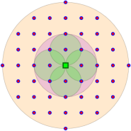
Figure 3.1: A tower can interact with at most 48 other towers.

If a tower has more than (say) $200/{\varepsilon}$ disks in it, then we add the greedy matching in the tower to the output, and remove all the disks in the tower. This yields a matching of size at least $100/{\varepsilon}$, that destroys at most $48$ additional edges from the optimal matching. Thus, it is sufficient to compute the approximate matching in the residual graph. We repeat this process till all the remaining towers have at most $O(1/{\varepsilon})$ disks in them. Let $\mathcal{D}^{\prime}$ be the remaining set of disks – by the bounded depth, each disk intersects at most $O(1/{\varepsilon})$ other disks, and the intersection graph of $G=\mathcal{I}_{\mathcal{D}^{\prime}}$ has $|E\left({G}\right)|=O(n/{\varepsilon})$ edges, and can be computed in $O(n/{\varepsilon})$ time. Using the algorithm of Duan and Pettie [DP14] on $\mathcal{I}_{\mathcal{D}^{\prime}}$, computing a $(1-{\varepsilon}/2)$-approximate matching takes $O(|E\left({G}\right)|{\varepsilon}^{-1}\log{\varepsilon}^{-1})=O(n{\varepsilon}^{-2}\log{\varepsilon}^{-1})$ time. It is straightforward to verify that this matching, together with the greedy matching of the “tall” towers yields that desired $(1-{\varepsilon})$-approximation.

As for the running for the case that the diameter $\Delta$ is relatively small – observe that after the cleanup step, there are at most $O(\Delta^{2})$ towers, and each tower contains $O(1/{\varepsilon})$ disks (each disk intersects $O(1/{\varepsilon})$ disks). As such, the residual graph has at most $O(\Delta^{2}/{\varepsilon}^{2})$ edges, and the running time of the Duan and Pettie [DP14] algorithm is $O\bigl{(}(\Delta^{2}/{\varepsilon}^{3})\log(1/{\varepsilon})\bigr{)}$.  

Using a reduction of Bonnet et al. [BCM20], we can reduce the residual graph even further, resulting in a slightly faster algorithm.

Lemma 3.3.

Let $\mathcal{D}$ be a set of $n$ unit disks, and let ${\varepsilon}\in(0,1)$ be a parameter. One can compute, in $O\bigl{(}(n/{\varepsilon})\log(1/{\varepsilon})\bigr{)}$ time, an $(1-{\varepsilon})$-matching in $\mathcal{I}_{\mathcal{D}}$.

Proof:

The algorithm works as follows:

1. It performs tower reduction and computes a greedy matching $\mathcal{C}_{1}$, as in Lemma 3.2, by doing greedy matching on each tower, till each tower contains $O(1/{\varepsilon})$ disks. Let $\mathcal{D}^{\prime}$ be the set of remaining disks.

2. Computes the intersection graph $G$ of $\mathcal{D}^{\prime}$.

3. Extracts a subgraph $H$ of $G$ by keeping only a few vertices from each tower. More precisely, the algorithm performs the following for each pair of adjacent towers.

   The algorithm computes a greedy matching $\mathcal{W}$ between two adjacent towers, keeping at most $\lambda+1$ edges in this matching. All the edges in $\mathcal{W}$ are marked. Next, the algorithm marks up to $\lambda+1$ edges (not in the partial matching) from each node in $\mathcal{W}$, to vertices in the adjacent tower.

   In the end, a disk is kept if it is contained in a marked edge. Let $\mathcal{D}^{\prime\prime}$ be the resulting set of disks. The surplus of a tower, defined by a point $p$, is the difference between the number of disks in $\mathcal{D}^{\prime}$ that contains it, and the number of disks in $\mathcal{D}^{\prime\prime}$ that contains it (i.e., the number of disks the tower lost). If the surplus is odd, the algorithm adds an arbitrary vertex from the surplus to $\mathcal{D}^{\prime\prime}$ (reducing the surplus by one, and making it even). Let $H$ be the intersection graph of $\mathcal{D}^{\prime\prime}$.

4. $(1-{\varepsilon}/8)$-approximates a maximum matching $\mathcal{C}_{2}$ in $H$ using the algorithm of Duan and Pettie [DP14].

5. Computes a greedy matching $\mathcal{C}_{3}$ in $G-\mathsf{V}\left({\mathcal{C}_{2}}\right)$, by computing a greedy matching for each tower.

6. Returns the matching $\mathcal{C}_{1}\cup\mathcal{C}_{2}\cup\mathcal{C}_{3}$.

Recall that every tower intersects at most $\lambda=O(1)$ other towers, see Figure 3.1. A matching in $G$, where there is at most one edge between two towers, is a tower matching.

The key observation (due to Bonnet et al. [BCM20]) is that for a maximum tower matching in $G$, for each tower, the number of internal (to the tower) matching edges is at least half of the surplus value (i.e., all the surplus edges are “used” by internal matching edges). Thus, given such a tower matching in $G$, one can perform an exchange argument, to get a maximum matching of the same size in $H$ (after adjusting for the surplus matching). Indeed, one argues that any matching strictly between towers in $G$ can be realized in $H$, and then it can be supplemented to a maximum matching back in $G$ by adding matching of surplus edges. See Bonnet et al. [BCM20] for details. Thus, it is enough to compute a maximum matching in $H$ (or approximate it), and then do a greedy matching to get the desired approximation.

The graph $H$ has $O(n\lambda^{2})=O(n)$ edges. Thus, running the approximation algorithm of Duan and Pettie [DP14] on $H$ takes $O\bigl{(}(n/{\varepsilon})\log(1/{\varepsilon})\bigr{)}$ time.  

Remark 3.4.

If the set of disks of $\mathcal{D}$ has diameter $\Delta$, then the cleanup stage reduces the number of disks to $O(\Delta^{2}/{\varepsilon})$. Then one can involve the algorithm of Lemma 3.3. The resulting algorithm has running time $O\bigl{(}n+(\Delta^{2}/{\varepsilon}^{2})\log(1/{\varepsilon})\bigr{)}$.

Remark.

The above algorithm can be modified to work in similar time for shapes of similar size – the only non-trivial step is computing the intersection graph $H$. This involves taking all the shapes in a tower, and its neighboring towers, computing their arrangement, and extracting the intersection pairs. If this involves $\nu$ shapes, then this takes $O(\nu^{2})$ time. Each shape would be charged $O(\nu^{2}/\nu)$ amortized time, which results in $O(n/{\varepsilon})$ time, as $\nu=O(1/{\varepsilon})$. The rest of the algorithm remains the same.

3.3 Matching size estimation

Theorem 3.5.

Let $\mathcal{D}$ be a set of $n$ unit disks, and let ${\varepsilon}\in(0,1)$ be a parameter. One can output a number $Z$, such that $(1-{\varepsilon})\mathcalb{m}^{\star}\leq\mathop{\mathbb{E}}\!\left[{Z}\right]$ and $\mathop{\mathbb{P}}\!\left[{Z<(1+{\varepsilon})\mathcalb{m}^{\star}}\right]\geq 1-1/n^{O(1)}$, where $\mathcalb{m}^{\star}$ is the size of the maximum matching in $\mathcal{I}_{\mathcal{D}}$, where $\mathcal{I}_{\mathcal{D}}$ is the intersection graph of $\mathcal{D}$. The running time of the algorithm is $O(n+{\varepsilon}^{-6}\log{\varepsilon}^{-1}\log^{2}n)$.

Proof:

We randomly shift a grid of size length $\psi=\left\lceil{32/{\varepsilon}}\right\rceil$ over the plane, by choosing a random point $p\in[0,\psi]^{2}$. Formally, the $(i,j)$th cell in this grid is $p+(i\psi,j\psi)+[0,\psi]^{2}$, where $i,j$ are integers. For a pair of unit disks that intersect, with probability $\geq 1-{\varepsilon}/2$ they both fall into the interior of a single grid cell. As such, throwing away all the disks that intersect the boundaries of the shifted grid, the remaining set of disks $\mathcal{D}^{\prime}$, in expectation, has a matching of size at least $(1-{\varepsilon}/8)\mathcalb{m}^{\star}$.

For a grid cell $\Box$ in this shifted grid, let $\mathcal{D}_{\Box}$ be the set of disks of $\mathcal{D}$ that are fully contained in $\Box$. A grid cell $\Box$ is active if $\mathcal{D}_{\Box}$ is not empty. Let $\mathcal{B}$ be the set of active grid cells. For a cell $\Box\in\mathcal{B}$, let $\mathcalb{m}^{\star}_{\Box}$ be the size of the maximum matching in $\mathcal{I}_{\mathcal{D}_{\Box}}$. Using the algorithm of Lemma 3.1, compute in $O(n)$ time overall, for all $\Box\in\mathcal{B}$, a number $e_{\Box}$ such that $\mathcalb{m}^{\star}_{\Box}/2\leq e_{\Box}\leq\mathcalb{m}^{\star}_{\Box}$.

The task at hand is to estimate the sum $\sigma=\sum_{\Box\in\mathcal{B}}\mathcalb{m}^{\star}_{\Box}$, where $\sigma\leq\mathcalb{m}^{\star}$ and $\mathop{\mathbb{E}}\!\left[{\sigma}\right]\geq(1-{\varepsilon}/8)\mathcalb{m}^{\star}$. To this end, we use importance sampling to reduce the number of terms in the summation of $\sigma$ that need to be evaluated. Each term $\mathcalb{m}^{\star}_{\Box}$ is $1/2$-approximated by $e_{\Box}$, and thus applying the algorithm of Lemma 2.6, to these approximation, with $\xi={\varepsilon}/32$, $b=2$, $M=n$, and $\gamma=1/n^{10}$, we get that

$$t=O\left({b^{4}\xi^{-2}(\log\log M+\log\gamma^{-1})\log M}\right)=O({\varepsilon}^{-2}\log^{2}n)$$

terms need to be evaluated (exactly if possible, but a $(1-{\varepsilon}/16)$-approximation is sufficient) to get $1\pm{\varepsilon}/8$ estimate for $\sigma$. For each such cell, we apply the algorithm of Remark 3.4, to get $(1-{\varepsilon}/16)$-approximation. For a cell $\Box$ this takes $O\bigl{(}|\mathcal{D}_{\Box}|+(1/{\varepsilon}^{4})\log(1/{\varepsilon})\bigr{)}$ time. Summing over all these $t$ cells, the running time is $O\bigl{(}n+(t/{\varepsilon}^{4})\log(1/{\varepsilon})\bigr{)}$.  

4 Approximate maximum matching for general disks

4.1 The greedy algorithm

The following $1/2$-approximation algorithm works (with the same running time) for any simply connected shapes that are well-behaved.

Lemma 4.1.

Let $\mathcal{D}$ be a set of $n$ disks in the plane. One can compute a greedy matching $\mathcal{C}$ for $\mathcal{I}_{\mathcal{D}}$ in $O(n\log n)$ time. This matching $\mathcal{C}$ is a $1/2$-approximation – that is, $\left|{\mathcal{C}}\right|\geq\mathcalb{m}^{\star}/2$, where $\mathcalb{m}^{\star}$ is the size of the maximum cardinality matching in $\mathcal{I}_{\mathcal{D}}$.

Proof:

The greedy algorithm repeatedly discovers a pair of disks that intersect, add them to the matching, and delete them from $\mathcal{D}$. Naively implemented, this requires quadratic time. Instead, we use the standard sweeping algorithm for computing the arrangement of circles (i.e., the boundaries of the disks). The algorithm performs the sweeping of the plane by a vertical line from left to right. Here, as soon as the sweeping algorithm discovers an intersection, it deletes the two disks involved in the intersection, and reports this pair as an edge in the matching. Naturally, the algorithm deletes the disks from the $y$-structure and the sweeping queue. An intersection takes $O(\log n)$ time to handle, and there can be at most $O(n)$ intersections before the algorithm terminates. All other events takes $O(n\log n)$ time to handle overall.  

4.2 Approximation algorithm when the graph is sparse

Lemma 4.2.

Let $\mathcal{D}$ be a set of $n$ disks in the plane such that the intersection graph $\mathcal{I}_{\mathcal{D}}$ has $m$ edges. For a parameter ${\varepsilon}\in(0,1)$, one can compute, in $O\bigl{(}n\log n+(m/{\varepsilon})\log(1/{\varepsilon})\bigr{)}$ time, an $(1-{\varepsilon})$-matching in $\mathcal{I}_{\mathcal{D}}$.

Proof:

Computing the vertical decomposition of the arrangement $\mathcal{A}\left({\mathcal{D}}\right)$ can be done in $O(n\log n+m)$ randomized time, using randomized incremental construction [BCKO08], as the complexity of $\mathcal{A}\left({\mathcal{D}}\right)$ is $O(n+m)$. This readily generates all the edges that arise out of pairs of disks with intersecting boundaries.

The remaining edges are created by one disk being enclosed completely inside another disk. One can perform a DFS on the dual graph of this arrangement, such that whenever visiting a trapezoid, the traversal maintains the set of disks that contains it. This takes time linear in the size of the arrangement, since the list of disks containing a point changes by at most one element between two adjacent faces. Now, whenever visiting a vertical trapezoid that on its non-empty vertical wall on the left contains an extreme right endpoint of a disk $\Circle$, the algorithm reports all the disks that contains this face, as having an edge with $\Circle$. Since every edge is generated at most $O(1)$ times by this algorithm, it follows that its overall running time is $O(n\log n+m)$.

Now that we computed the intersection graph, we apply the algorithm of Duan and Pettie [DP14]. This takes $O\bigl{(}(m/{\varepsilon})\log(1/{\varepsilon})\bigr{)}$ time, and computes the desired matchings.  

The above is sufficient if the intersection graph is sparse, as is the case if the graph is low density.

Lemma 4.3.

Let $\mathcal{D}$ be a set of $n$ disks in the plane with density $\rho$. For a parameter ${\varepsilon}\in(0,1)$, one can $(1-{\varepsilon})$-approximate the maximum matching in $\mathcal{I}_{\mathcal{D}}$ in $O\bigl{(}n\log n+\frac{n\rho}{{\varepsilon}}\log\frac{1}{{\varepsilon}}\bigr{)}$ time.

Proof:

The smallest disk in $\mathcal{D}$ intersects at most $\rho$ other disks of $\mathcal{D}$. Removing this disk and repeating this argument, implies that $\mathcal{I}_{\mathcal{D}}$ has at most $\rho n$ edges. The result now readily follows from Lemma 4.2.  

4.3 The bipartite case

Consider computing maximum matching when given two sets of disks $\mathcal{D}_{1},\mathcal{D}_{2}$, where one considers only intersections between disks that belong to different sets – that is the bipartite case. Efrat et al. [EIK01] showed how to implement one round of Hopcroft-Karp algorithm using $O(n)$ dynamic range searching operations on a set of disks. Using the (recent) data-structure of Kaplan et al. [KMR+20], one can implement this algorithm. Each operation on the dynamic disks data-structure takes $O(\log^{11}n)$ time. If our purpose is to get an $(1-{\varepsilon})$-approximation, we need to run this algorithm $O(1/{\varepsilon})$ times, so that all paths of length $O(1/{\varepsilon})$ get augmented, resulting in the following.

Lemma 4.4.

Given sets $\mathcal{D}_{1},\mathcal{D}_{2}$ at most $n$ disks in he plane, one can $(1-{\varepsilon})$-approximate the maximum matching in the bipartite graph

$$\mathcal{I}_{\mathcal{D}_{1},\mathcal{D}_{2}}=(\mathcal{D}_{1}\cup\mathcal{D}_{2},\left\{\Circle_{1}\Circle_{2}\;\middle|\;\Circle_{1}\in\mathcal{D}_{1},\Circle_{2}\in\mathcal{D}_{2},\text{ and }\Circle_{1}\cap\Circle_{2}\neq\emptyset\right\}).$$

in $O\bigl{(}(n/{\varepsilon})\log^{11}n\bigr{)}$ time. Any augmenting path for this matching has length at least $4/{\varepsilon}$.

4.4 Approximate matching via reduction to the bipartite case

We use a reduction, due to Lotker et al. [LPP15], of approximate general matchings to the bipartite case.

4.4.1 The Algorithm

The input is a set $\mathcal{D}$ of $n$ disks, and a parameter ${\varepsilon}\in(0,1)$. The algorithm maintains a matching $\mathcal{C}$ in $\mathcal{I}_{\mathcal{D}}$. Initially, this matching can be the greedy matching. Now, the algorithm repeats the following $O(c_{\varepsilon}\log n)$ times, where $c_{\varepsilon}=2^{8/{\varepsilon}}$:

$i$th iteration: Randomly color the disks of $\mathcal{D}$ by two colors (say $1$ and $2$), and let $\mathcal{D}_{1},\mathcal{D}_{2}$ be the resulting partition. Remove from $\mathcal{D}_{1}$ any pair of disks $\Circle_{1},\Circle_{2}$ such that $\Circle_{1}\Circle_{2}$ is in the current matching $\mathcal{C}$. Do the same to $\mathcal{D}_{2}$. Let $\mathcal{C}_{i}^{\prime}$ be edges of $\mathcal{C}$ that appear in $H_{i}=\mathcal{I}_{\mathcal{D}_{1},\mathcal{D}_{2}}$. Using Lemma 4.4, find an $(1-{\varepsilon}/16)$-approximate maximum matching in $H_{i}$, and let $\mathcal{C}_{i}^{\prime\prime}$ be this matching. Augment $\mathcal{C}$ with the augmenting paths in $\mathcal{C}_{i}^{\prime}\oplus\mathcal{C}_{i}^{\prime\prime}$.

The intuition behind this algorithm is that this process would compute all the augmenting paths of $\mathcal{C}$ of length (say) $\leq 4/{\varepsilon}$, which implies that the resulting matching is the desired approximation.

4.4.2 Analysis

Lemma 4.5.

The above algorithm outputs a matching of size $\geq(1-{\varepsilon})\mathcalb{m}^{\star}$, with probability $\geq 1-1/n^{O(1)}$.

Proof:

Let $\mathcal{M}^{\star}$ denote the maximum cardinality matching in $\mathcal{I}_{\mathcal{D}}$ (thus, $\mathcalb{m}^{\star}=|\mathcal{M}^{\star}|$). We group the iterations of the algorithm into epochs. An epoch is a consecutive blocks of $\gamma=4\cdot 2^{4/{\varepsilon}}$ iterations. Let $\mathcal{C}_{i}$ be the matching computed by the algorithm in the beginning of the $i$th epoch. Let $d_{i}=\mathcalb{m}^{\star}-|\mathcal{C}_{i}|$ be the deficit from the optimal solution in the beginning of the $i$th epoch. Initially $d_{1}\leq\mathcalb{m}^{\star}/2$. Let $T_{i}$ be a maximum cardinality set of augmenting paths for $\mathcal{C}_{i}$, such that each path is of length at most

$$\tau=4/{\varepsilon}.$$

By Lemma 2.8, we have $|T_{i}|\geq({\varepsilon}/2)\mathcalb{m}^{\star}$.

Fix a specific path $\pi\in T_{i}$. A random coloring by two colors, has probability $p\geq 1/2^{\tau}$ to color $\pi$ such that the colors of the disks are alternating. The path $\pi$ is destroyed in an iteration during the epoch, if the algorithm augments along a path that intersects $\pi$. If $\pi$ is colored in alternating colors in, then it must have been destroyed (in this or earlier iteration) by the algorithm of Lemma 4.4 as it extracts a set of augmenting paths, and after it is applied, all remaining augmenting paths have length (say) $\geq 8/{\varepsilon}$ (which is longer then $\pi$).

It follows that after $\gamma$ iterations in the epoch, the probability of a path of $T_{i}$ to survive is at most $(1-p)^{\gamma}=(1-p)^{4/p}\leq\exp(-4)\leq 1/50$. Let $Z_{i}$ be the number of paths of $T_{i}$ that survive the $i$th epoch. We have that $\mathop{\mathbb{E}}\!\left[{Z_{i}}\right]\leq|T_{i}|/50$. The $i$th epoch is successful if at least half the paths of $T_{i}$ are destroyed in this epoch. By Markov’s inequality, we have

$$\mathop{\mathbb{P}}\!\left[{i\text{th epoch is a failure}}\right]=\mathop{\mathbb{P}}\!\left[{Z_{i}>|T_{i}|/2}\right]<\frac{\mathop{\mathbb{E}}\!\left[{Z_{i}}\right]}{|T_{i}|/2}=\frac{1}{25}.$$

If the $i$th epoch is successful, then it computes at least $|T_{i}|/(2\tau)\geq({\varepsilon}^{2}/10)\mathcalb{m}^{\star}$ augmenting paths, which implies that $d_{i+1}\leq d_{i}-({\varepsilon}^{2}/10)\mathcalb{m}^{\star}$. In particular, the algorithm must reach the desired approximation after $10/{\varepsilon}^{2}$ successful epochs. Since the success of the epochs are independent events, it follows, with high probability, that the algorithm must collect the desired number of successful epochs, after $O({\varepsilon}^{-2}+\log n)$ epochs – this follows readily from Chernoff’s inequality, see Lemma A.2.

Finally, observe that $O(4\cdot 2^{4/{\varepsilon}}/{\varepsilon}^{2})=2^{8/{\varepsilon}}$.  

4.4.3 The result

Theorem 4.6.

Let $\mathcal{D}$ be a set of $n$ disks in the plane, and ${\varepsilon}\in(0,1)$ be a parameter. One can compute a matching in $\mathcal{I}_{\mathcal{D}}$ of size $\geq(1-{\varepsilon})\mathcalb{m}^{\star}$, in $O(2^{8/{\varepsilon}}n\log^{12}n)$ time, where $\mathcalb{m}^{\star}$ is the cardinality of the maximum matching in $\mathcal{I}_{\mathcal{D}}$. The algorithm succeeds with high probability.

Remark.

Note, that the above algorithm does not work for fat shapes (even of similar size), since the range searching data-structure of Kaplan et al. [KMR+20] can not to be used for such shapes.

4.5 Algorithm for the case the maximum matching is small

If $n_{\mathcal{C}}=\left|{\mathcal{C}}\right|$ is small (say, polylogarithmic), it turns out that one can compute the maximum matching exactly in near linear time.

Lemma 4.7.

For a set $X$ of $n$ disks, and any constant $\delta\in(0,1)$, one can preprocess $X$, in $O(n^{3+\delta}\log n)$ time, such that given a query disk $\Circle$, the algorithm outputs, in $O(\log n)$ time, a pointer to a (unique) list containing all the disks intersecting the query disk.

Proof:

Map a disk centered at $(x,y)$ and radius $r$ in $X$ to the $45^{\circ}$ cone in three dimensions with axis parallel to the $z$-axis and with an apex at $(x,y,-r)$. Observe that this cone intersects the $xy$-plane at a circle that forms the boundary of the original disk. A new disk centered at $(x^{\prime},y^{\prime})$ of radius $r^{\prime}$ intersects the original disk $\iff$ $(x^{\prime},y^{\prime},r^{\prime})$ lies above this cone. Thus, every set in $\mathcal{R}$ is a face in the arrangement of $n$ cones induced by the disks of $X$. This arrangement has $O(n^{3})$ faces/vertices/edges. The second result follows by preprocessing this arrangement to point location [AM00] - this takes $O(n^{3+\delta})$ time, and a point-location query takes $O(\log n)$ time, where $\delta\in(0,1)$ is an arbitrary fixed constant.  

Lemma 4.8.

Let $\mathcal{D}$ be a set of $n$ disks in the plane. Then, in $O(n\log n)$ time, one can decide if $\mathcalb{m}^{\star}\left({\mathcal{D}}\right)=O(n^{1/8})$, and if so compute and output this maximum matching.

Proof:

Let $N=cn^{1/8}$, where $c$ is some sufficiently large constant. Compute a greedy matching $\mathcal{C}$ in $\mathcal{I}_{\mathcal{D}}$ using the algorithm of Lemma 4.1. If $\left|{\mathcal{C}}\right|>N$, then the maximum matching is larger than desired, and the algorithm is done.

Otherwise, let $F=\mathcal{D}\setminus\mathsf{V}_{\mathcal{C}}$, where $\mathsf{V}_{\mathcal{C}}$ is the set of vertices of $\mathcal{C}$. The set $F$ is independent, as $\mathcal{C}$ is a greedy matching. Preprocessing the elements of $\mathsf{V}_{\mathcal{C}}$ using the data-structure of Lemma 4.7, we can partition the disks of $F$ into $O(N^{3})$ classes, where all the disks in the same class intersects exactly the same subset of disks of $\mathcal{C}$. Furthermore, doing point location query for the lifted point, corresponding to each disk of $F$, one can decide identify its class in $O(\log n)$ time. Observe that all the vertices in the same class have exactly the same neighbors in $\mathcal{I}_{\mathcal{D}}$. This takes $O(N^{3+\delta}+n\log n)=O(n\log n)$ time.

Observe that the maximum matching can use at most $2N$ vertices that belongs to the same class. Thus, classes that exceed this size can be trimmed to this size. Let $\mathcal{D}^{\prime}$ be the resulting set of disks, and observe that $\left|{\mathcal{D}^{\prime}}\right|=O(N^{3}\cdot N)=O(N^{4})$. Observe that $\mathcal{D}^{\prime}$ has the same cardinality maximum matching as $\mathcal{D}$. Furthermore, the graph $G^{\prime}=\mathcal{I}_{\mathcal{D}^{\prime}}$ has at most $m=O(N^{5})$ edges.

Using the maximum cardinality matching algorithm of Gabow and Tarjan on $G^{\prime}$, takes $O(\sqrt{m}|\mathcal{D}^{\prime}|)=O(N^{5/2+4})=o(n)$. We return this as the desired maximum matching.  

4.6 Estimation of matching size using separators

The input is a set $\mathcal{D}$ of $n$ disks in the plane with density $\rho$ (if the value of $\rho$ is not given, it can be approximated in near linear time [AH08]). Our purpose here is to $(1-{\varepsilon})$-estimate the size of the maximum matching in $\mathcal{D}$ in near linear time. Since we can check (and compute it) if the maximum matching is smaller than $n^{1/8}$ by Lemma 4.8, in $O(n\log n)$ time, assume that the matching is bigger than that.

4.6.1 Preliminaries

Lemma 4.9 ([Har13]).

Let $p$ be a point in the plane, and let $r$ be a random number picked uniformly in an interval $[\alpha,2\alpha]$. Let $\mathcal{H}$ be a set of interior disjoint disks in the plane. Then, the expected number of disks of $\mathcal{H}$ that intersects the circle $\Circle=\Circle(p,r)$, that is centered at $p$ and has radius $r$, is $O(\sqrt{\left|{\mathcal{H}}\right|})$.

Proof:

We include the proof for the sake of completeness. For simplicity of exposition, translate and scale the plane so that $p$ is in the origin, and $\alpha=1$. Next, cover the square $S=[-3,3]^{2}$ by a grid of sidelength $\ell=1/10$, and let $P$ be the set of points formed by the vertices of this grid. We have $|P|=O(1/\ell^{2})=O(1)$. The number of disks of $\mathcal{H}$ that contains points of $P$ is bounded by $|P|$. Any other disk of $\mathcal{H}$ that intersects $\Circle$, must be of radius $\leq 1/2$, and is fully contained inside $S$. In particular, let $D_{1},\ldots,D_{m}$ be these disks, with $r_{1},\ldots r_{m}$ being their radii, respectively. Observe that $\sum_{i}\pi r_{i}^{2}\leq\mathrm{area}(S)=36.$ and the probability of the $i$th disk to intersect $\Circle$ is at most $2r_{i}/\alpha=2r_{i}$. As such, the expected number of disks of $\mathcal{H}$ intersecting $\Circle$ is bounded by $|P|+\sum_{i=1}^{m}2r_{i}.$ However, by the Cauchy-Schwarz inequality, we have $\sum_{i=1}^{m}r_{i}\leq\sqrt{\sum_{i=1}^{m}1^{2}}\sqrt{\sum_{i=1}^{m}r_{i}^{2}}\leq\sqrt{m}\sqrt{36/\pi}=O(\sqrt{\left|{\mathcal{H}}\right|}),$ as $m\leq\left|{\mathcal{H}}\right|$.  

4.6.2 Algorithm idea and divisions

A natural approach to our problem is to break the input set of disks into small sets, and then estimate the maximum matching size in each one of them. The problem is that for this to work, we need to partition the disks participating in the optimal matching, as this matching can be significantly smaller than the number of input disks. Since we do not have the optimal matchings, we would use a proxy to this end – the greedy matching. The algorithm recursively partitions it using a random cycle separator provided by Lemma 2.5. We then partition the disks into three sets – inside the cycle, intersecting the cycle (i.e., the separator), and outside the cycle. The algorithm continues this partition recursively on the in/out sets, forming a partition hierarchy.

Remark 4.10.

For a set generated by this partition, its boundary is the set of all disks that intersect it and are not in the set. The algorithm maintains the property that for such a set with $t$ disks, the number of its boundary vertices is bounded by $O(\rho+\sqrt{\rho t})$. This can be ensured by alternately separating for cardinality of the set, and for the cardinality of the boundary vertices, see [HQ17] and references therein for details. For simplicity of exposition we assume this property holds, without going into the low level details required to ensure this.

4.6.3 The algorithm

The input is a set $\mathcal{D}$ of $n$ disks in the plane with density $\rho$, and parameters ${\varepsilon}\in(0,1)$. The algorithm computes the greedy matching, denoted by $\mathcal{C}$, using Lemma 4.1. If this matching is smaller than $O(n^{1/8})$, then the algorithm computes the maximum matching using Lemma 4.8, and returns it.

Otherwise, the algorithm partitions the disks of $\mathcal{H}=\mathsf{V}\left({\mathcal{C}}\right)$ recursively using separators, creating a separator hierarchy as described above. Conceptually, a subproblem here is a region $R$ in the plane formed by the union of some faces in an arrangement of circles (i.e., the separators used in higher level of the recursion). Assume the algorithm has the sets of disks $\mathcal{H}_{\subseteq R}=\left\{\Circle\in\mathcal{H}\;\middle|\;\Circle\subseteq R\right\}$ and $\mathcal{D}_{\subseteq R}=\left\{\Circle\in\mathcal{D}\;\middle|\;\Circle\subseteq R\right\}$ at hand. The algorithm computes a separator of $\mathcal{H}_{\subseteq R}$, computes the relevant sets for the children, and continues recursively on the children. Thus, for a node $u$ in this recursion tree, there is a corresponding region $R(u)$, a set of active disks $\mathcal{H}_{u}=\mathcal{H}_{\subseteq R(u)}$, and $\mathcal{D}_{u}=\mathcal{D}_{\subseteq R(u)}$.

The recursion stops the construction in node $u$ if $|\mathcal{H}_{u}|\leq b$, where

$$b=\mathsf{c}_{3}\rho/{\varepsilon}^{2},$$

and $\mathsf{c}_{3}$ is some sufficiently large constant. This implies that this recursion tree has $U=O(\mathcalb{m}^{\star}/b)$ leafs.

If a disk of $\mathcal{D}$ intersects some separator cycles then it is added to the set of “lost” disks $\mathcal{L}$. The hierarchy maps every disk of $\mathcal{D}\setminus\mathcal{L}$ to a leaf. As such, for every leaf $u$ of the separator tree, there is an associated set $\mathcal{D}_{u}$ of disks stored there. All these leaf sets, together with $\mathcal{L}$, form a disjoint partition of $\mathcal{D}$.

The algorithm now computes for every leaf set a greedy matching, using Lemma 4.1. Let $e_{v}$ be the size of this matching. Let $\Xi$ be the set of all leaf nodes. The algorithm next $(1\pm{\varepsilon}/4)$-estimates $\sum_{v\in\Xi}\mathcalb{m}^{\star}\left({\mathcal{D}_{v}}\right)$, using importance sampling, with the estimates $e_{v}\leq\mathcalb{m}^{\star}\left({\mathcal{D}_{v}}\right)\leq 2e_{v}$, for all $v$. Using, Lemma 2.6, this requires computing $(1-{\varepsilon}/8)$-approximate maximum matching for

$$t=O\left({2^{4}{\varepsilon}^{-2}(\log\log n+\log n)\log n}\right)=O({\varepsilon}^{-2}\log^{2}n)$$

leafs, this is done using the algorithm of Lemma 4.8 if the maximum matching is small compared to the number of disks in this subproblem, and the algorithm of Lemma 4.3 otherwise. The algorithm now returns the estimate returned by the algorithm of Lemma 2.6.

4.6.4 Analysis

Lemma 4.11.

We have $\mathop{\mathbb{E}}\!\left[{\sum_{v\in L}\mathcalb{m}^{\star}\left({\mathcal{D}_{v}}\right)}\right]\geq(1-{\varepsilon}/4)\mathcalb{m}^{\star}\left({\mathcal{D}}\right)$.

Proof:

Let $\zeta\in(0,1)$ be the constant (that does not depend on the density) from Lemma 2.5 – in two dimensions $\zeta\approx 9/10$ [Har13]. The depth of the recursion of the above algorithm is $h=O\bigl{(}1+\log_{1/\zeta}({2\left|{\mathcal{C}}\right|}/{b})\bigr{)}=O(\log\tfrac{\mathcalb{m}^{\star}}{{\varepsilon}^{2}}).$

The expected number of disks of $\mathcal{H}$ (and thus edges of $\mathcal{C}$) destroyed by this process is

$$\sum_{i=0}^{h}2^{i}O\left({\rho+\rho^{1/2}(2\mathcalb{m}^{\star}\zeta^{i})^{1/2}}\right).$$

This is a geometric summation dominated by the last term – that is, the total loss is bounded by the loss in the parents of the leafs of the recursion multiplied by (say) eight. Let $N=O(\mathcalb{m}^{\star}/b)$ be the number of leafs in the recursion tree. The loss in the leafs is bounded by

$$\lambda=N\cdot O\left({\rho+\sqrt{\rho b}}\right)=O\left({\frac{2|\mathcal{H}|\sqrt{\rho b}}{b}}\right)=O\left({\frac{\mathcalb{m}^{\star}\sqrt{\rho}}{\sqrt{\mathsf{c}_{3}\rho/{\varepsilon}^{2}}}}\right)=O\left({\frac{{\varepsilon}}{\sqrt{\mathsf{c}_{3}}}\mathcalb{m}^{\star}}\right)<\frac{{\varepsilon}}{64}\mathcalb{m}^{\star},$$

by making $\mathsf{c}_{3}$ sufficiently large. Specifically, let $\mathcal{H}^{\prime}$ be the disks of $\mathcal{H}$ that do not intersect any of the circles in the separator hierarchy – we have that the expected loss is $\ell=\mathop{\mathbb{E}}\!\left[{\left|{\mathcal{H}\setminus\mathcal{H}^{\prime}}\right|}\right]\leq 8\lambda\leq{\varepsilon}\mathcalb{m}^{\star}/8$.

Let $\mathsf{V}^{\star}=\mathsf{V}\left({\mathcal{M}^{\star}}\right)$, and let $F=\mathcal{D}\setminus\mathcal{H}$. As the disks in $\mathcal{H}$ are the vertices of a maximum matching, it follows that $F$ is an independent set. The number of vertices of $F$ that intersects the separating circles of the separation hierarchy can be arbitrarily larger than $\mathcalb{m}^{\star}$. But fortunately, for our purposes, we care only about bounding the number of disks of $\mathsf{V}^{\star}$ intersecting these cycles. To this end, observe that the expected loss in $\mathsf{V}^{\star}\cap\mathcal{H}$ is bounded by $\ell$. As such, we remain with the task of bounding the loss in $\mathsf{V}^{\star}\cap F$. So consider the separator in the top of the hierarchy. By Lemma 4.9, the expected number of vertices of $\mathsf{V}^{\star}\cap F$ that intersect it, is bounded by $O\bigl{(}\sqrt{\left|{\mathsf{V}^{\star}\cap F}\right|}\bigr{)}=O(\sqrt{\mathcalb{m}^{\star}})$. However, this quantity is smaller than the number of disks of $\mathcal{H}$ being cut by this separator. Repeating (essentially) the same calculations as above, we get that the total expected number of disks of $\mathsf{V}^{\star}\cap F$ cut by the cycles of the separator hierarchy is also bounded by $\ell$.

The above claim requires some care – a subproblem at a node $u$ has the set of vertices from the greedy matching $k_{u}=|\mathcal{H}_{u}|$. Importantly, the boundary set for $u$ has size $t=O(\sqrt{k_{u}})$, see Remark 4.10. As such, a maximal matching in this subproblem (even if we include all the disks intersecting the boundary) is of size at most $k_{u}+t$. Indeed, every one of the boundary disks of the greedy matching might now be free to be engaged to a different disk in this subproblem (we use here the property that all the disks not in the greedy matching are independent). The maximum matching can be at most twice the size of the greedy matching, which imply that the maximum matching size for $\mathcal{D}_{u}$ is bounded by (say) $2(k_{u}+t)\leq 3k_{u}$, which implies that the above bounding argument indeed works.

Combining the two expected bounds on the size of $\mathcal{L}\cap\mathsf{V}^{\star}\cap F$ and $\mathcal{L}\cap\mathsf{V}^{\star}\cap\mathcal{H}$ implies that in expectation, summed over all the leafs, the maximum matching, has at least $\mathcalb{m}^{\star}-2\ell$ edges, which in expectation is $\geq(1-{\varepsilon}/4)\mathcalb{m}^{\star}$. This implies that the “surviving” maximum matching in the leafs is a good approximation to the maximum matching.  

Lemma 4.12.

The running time of the above algorithm is $O(n\log n+\rho^{9}{\varepsilon}^{-19}\log^{2}n)$.

Proof:

The separator hierarchy takes $O(n\log n)$ time to build. So, consider the $t=O({\varepsilon}^{-2}\log^{2}n)$ subproblems. If the $i$th subproblem has $n_{i}$ disks, and $n_{i}\geq b^{8}$, then computing the maximum matching for this subproblem takes $O(n_{i}\log n_{i})$ time. Otherwise, it takes $O(n_{i}\log n_{i}+n_{i}\rho/{\varepsilon})=O(n_{i}\log n_{i}+b^{8}\rho/{\varepsilon})=O(n_{i}\log n_{i}+\rho^{9}/{\varepsilon}^{17}).$ Summing over all $t$ subproblems, this takes $O(n\log n+t\rho^{9}/{\varepsilon}^{17})=O(n\log n+\rho^{9}{\varepsilon}^{-19}\log^{2}n)$.  

Theorem 4.13.

Given a set $\mathcal{D}$ of $n$ disks in the plane with density $\rho$, and a parameter ${\varepsilon}\in(0,1)$, one can compute in $O(n\log n+\rho^{9}{\varepsilon}^{-19}\log^{2}n)$ time, a number $Z$, such that $(1-{\varepsilon})\mathcalb{m}^{\star}\leq\mathop{\mathbb{E}}\!\left[{Z}\right]$ and $\mathop{\mathbb{P}}\!\left[{Z>(1+{\varepsilon})\mathcalb{m}^{\star}}\right]<1/n^{O(1)},$ where $\mathcalb{m}^{\star}=\mathcalb{m}^{\star}\left({\mathcal{D}}\right)$ is the size of the maximum matching in $\mathcal{I}_{\mathcal{D}}$.

Proof:

The result follows from the above, adding in the guaranties provided by the importance sampling.  

Appendix A Chernoff inequality

The following is a standard version of Chernoff inequality.

Theorem A.1.

Let $X_{1},\ldots,X_{n}$ be $n$ independent coin flips, such that $\mathop{\mathbb{P}}\!\left[{X_{i}=0}\right]=\mathop{\mathbb{P}}\!\left[{X_{i}=1}\right]=\frac{1}{2}$, for $i=1,\ldots,n$. Let $Y=\sum_{i=1}^{n}X_{i}$. Then, for any $\Delta>0$, we have $\mathop{\mathbb{P}}\!\left[{Y\leq{n}/{2}-\Delta}\right]\leq\exp\left({-2\Delta^{2}/n}\right).$

Lemma A.2.

Let $M>0$ and $n$ be positive integer parameters. Consider performing $u=2c\left\lceil{\ln n}\right\rceil+4M$ independent experiments, where each experiments succeeds with probability $\geq 1/2$. Then, with probability $\geq 1/n^{c}$, at least $M$ of these experiments succeeded.

Proof:

Let $X_{i}$ be one of the $i$th experiment succeeded, and let $Y=\sum_{i}X_{i}$ – we assume here that $X_{i}$ has exactly probability $1/2$ to success, and $c>2$ is a prespecified constant. By Theorem A.1, we have that the probability of failure is

$$\mathop{\mathbb{P}}\!\left[{Y<M}\right] =\mathop{\mathbb{P}}\!\left[{Y<M}\right]=\mathop{\mathbb{P}}\!\left[{Y\leq(c\left\lceil{\ln n}\right\rceil+2M)-c\left\lceil{\ln n}\right\rceil-M}\right]\leq\exp\left({-2\frac{(c\left\lceil{\ln n}\right\rceil+M)^{2}}{2c\left\lceil{\ln n}\right\rceil+4M}}\right)$$

$$\leq\exp\left({-2\frac{(c\left\lceil{\ln n}\right\rceil+M)^{2}}{4\left({c\left\lceil{\ln n}\right\rceil+M}\right)}}\right)\leq\frac{1}{n^{c}}.$$

References

- [AH08] Boris Aronov and Sariel Har-Peled “On Approximating the Depth and Related Problems” In SIAM J. Comput. 38.3 SIAM, 2008, pp. 899–921 DOI: 10.1137/060669474
- [AM00] P.. Agarwal and M. “Arrangements and their applications” In Handbook of Computational Geometry Amsterdam: North-Holland Publishing Co., 2000, pp. 49–119 URL: http://www.cs.duke.edu/~pankaj/papers/arrangement-survey.ps.gz
- [BCKO08] Mark Berg, Otfried Cheong, Marc J. Kreveld and Mark H. Overmars “Computational Geometry: Algorithms and Applications” Santa Clara, CA, USA: Springer, 2008 DOI: 10.1007/978-3-540-77974-2
- [BCM20] Édouard Bonnet, Sergio Cabello and Wolfgang Mulzer “Maximum Matchings in Geometric Intersection Graphs” In Proc. 37th Internat. Sympos. Theoret. Asp. Comp. Sci. (STACS) 154, LIPIcs Schloss Dagstuhl - Leibniz-Zentrum für Informatik, 2020, pp. 31:1–31:17 DOI: 10.4230/LIPIcs.STACS.2020.31
- [BHR+20] Paul Beame et al. “Edge Estimation with Independent Set Oracles” In ACM Trans. Algo. 16.4 New York, NY, USA: Association for Computing Machinery, 2020 DOI: 10.1145/3404867
- [DP14] Ran Duan and Seth Pettie “Linear-Time Approximation for Maximum Weight Matching” In J. ACM 61.1 New York, NY, USA: Association for Computing Machinery, 2014 DOI: 10.1145/2529989
- [EIK01] Alon Efrat, Alon Itai and Matthew J. Katz “Geometry Helps in Bottleneck Matching and Related Problems” In Algorithmica 31.1, 2001, pp. 1–28 DOI: 10.1007/s00453-001-0016-8
- [GT91] Harold N. Gabow and Robert Endre Tarjan “Faster Scaling Algorithms for General Graph-Matching Problems” In J. Assoc. Comput. Mach. 38.4, 1991, pp. 815–853 DOI: 10.1145/115234.115366
- [Har09] Nicholas J.. Harvey “Algebraic Algorithms for Matching and Matroid Problems” In SIAM J. Comput. 39.2, 2009, pp. 679–702 DOI: 10.1137/070684008
- [Har13] Sariel Har-Peled “A Simple Proof of the Existence of a Planar Separator” In ArXiv e-prints, 2013 arXiv:1105.0103 [cs.CG]
- [HK73] John E. Hopcroft and Richard M. Karp “An Algorithm for Maximum Matchings in Bipartite Graphs” In SIAM J. Comput. 2.4, 1973, pp. 225–231 DOI: 10.1137/0202019
- [HQ17] Sariel Har-Peled and Kent Quanrud “Approximation Algorithms for Polynomial-Expansion and Low-Density Graphs” In SIAM J. Comput. 46.6, 2017, pp. 1712–1744 DOI: 10.1137/16M1079336
- [HY22] Sariel Har-Peled and Everett Yang “Approximation Algorithms for Maximum Matchings in Geometric Intersection Graphs” In CoRR abs/2201.01849, 2022 arXiv: https://arxiv.org/abs/2201.01849
- [KMR+20] Haim Kaplan et al. “Dynamic Planar Voronoi Diagrams for General Distance Functions and Their Algorithmic Applications” In Discrete Comput. Geom. 64.3 Springer ScienceBusiness Media LLC, 2020, pp. 838–904 DOI: 10.1007/s00454-020-00243-7
- [LPP15] Zvi Lotker, Boaz Patt-Shamir and Seth Pettie “Improved Distributed Approximate Matching” In J. Assoc. Comput. Mach. 62.5, 2015, pp. 38:1–38:17 DOI: 10.1145/2786753
- [MS04] Marcin Mucha and Piotr Sankowski “Maximum Matchings via Gaussian Elimination” In Proc. 45th Annu. IEEE Sympos. Found. Comput. Sci. (FOCS) IEEE Computer Society, 2004, pp. 248–255 DOI: 10.1109/FOCS.2004.40
- [MS06] Marcin Mucha and Piotr Sankowski “Maximum Matchings in Planar Graphs via Gaussian Elimination” In Algorithmica 45.1, 2006, pp. 3–20 DOI: 10.1007/s00453-005-1187-5
- [YZ07] Raphael Yuster and Uri Zwick “Maximum matching in graphs with an excluded minor” In Proc. 18th ACM-SIAM Sympos. Discrete Algs. (SODA) SIAM, 2007, pp. 108–117 URL: http://dl.acm.org/citation.cfm?id=1283383.1283396