Non-destructive mapping of stress, strain and stiffness of thin elastically deformed materials
Abstract
Knowing the stress within a soft material is of fundamental interest to basic research and practical applications, such as soft matter devices, biomaterial engineering, and medical sciences. However, it is challenging to measure stress fields in situ in a non-invasive way. It becomes even more difficult if the mechanical properties of the material are unknown or altered by the stress. Here we present a robust non-destructive technique capable of measuring in situ stress and strain in elastically deformed thin films without the need to know their material properties. The technique is based on measuring elastic wave speeds, and then using a universal dispersion curve we derived for Lamb wave to predict the local stress and strain. Using optical coherence tomography, we experimentally verified the method for a rubber sheet, a cling film, and the leather skin of a musical instrument.
keywords: Mechanical stress Lamb wave Acoustoelasticity Optical coherence elastography Soft matter
Introduction
Soft thin films hanging in the air or confined in fluids are ubiquitous in our daily lives as well as in natural and engineering systems. Examples include cling film packaging food, the eardrum and the diaphragm in our body, and various elastic sheets, membranes, vesicles and bands holding structures together. They are typically under external and internal stress, and it is often desirable to know the stress level to be able to understand the environment they are exposed to or interacting with, or to monitor the changes in and health of the materials. However, in situ non-invasive measurements of the stress are challenging. This is even more challenging if the mechanical properties of the material are unknown and, furthermore, if the original configuration of the material is unknown, which precludes straightforward measurement of strain [1, 2].
Various techniques have been devised to measure in-plane stresses [3]. The choice of technique depends on the material type (solid/liquid/type of molecules) and also on the length scale. Essentially all techniques so far rely on the knowledge of the elastic moduli of the material or some specific expected behaviour of the material, which limits their application to known or specific materials and structures. For example, in the Langmuir–Blodgett trough [4], a workhorse of membrane biophysics, surface tension is estimated by measuring the amount of force required to insert a Wilhelmy plate into a given membrane. However, this force depends on the nature of the surface tension and its accuracy has been questioned for solid-like membranes [5]. Conventional ultrasound methods also require the elastic moduli and acousto-elastic parameters of the materials to predict the stress [6, 12].
Here we describe a technique that allows the stress field to be determined in soft thin films even without a priori knowledge of the material properties or applied strain. The technique uses Lamb elastic waves propagating in the film [7, 8] followed by a simple algorithm to determine the stress from measured wave speeds. In this work, we use optical coherence tomography (OCT) to visualise the elastic waves and measure their propagation speeds in an audible frequency range. This range (1-20 kHz) is well suited for soft materials with thickness ranging from sub-micron to a few hundreds of micrometers.
Results
Theoretical foundation
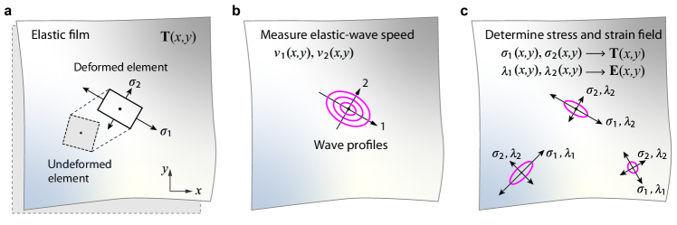
Figure 1 illustrates the general principle for a film under an arbitrary stress field T which deformed it elastically. The local wave speed is affected not only by the stiffness of the material but also by the direction and magnitude of the local stress (Fig. 1b) [9]. The two principal stresses and and stretch ratios and , at a location are related to the in-plane stress (Cauchy stress) and strain (Green-Lagrange strain) at the location (Fig. 1c). Mathematically, and are obtained by diagonalising the stress tensor.
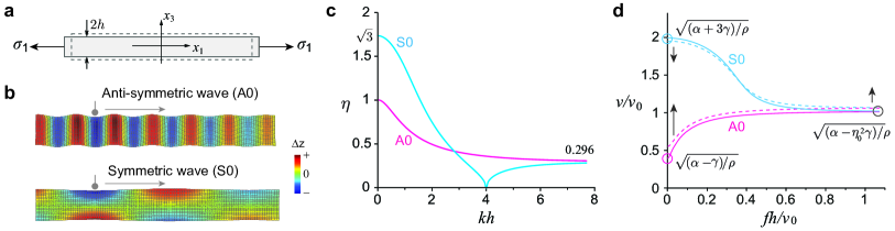
To develop our algorithm, we consider a deformed element (Fig. 2a) with local coordinates , where , being the thickness. The film is subject to the in-plane stresses and along the and axes, respectively, and the out-of-plane stress along the axis ( in thin films). An infinitesimal elastic wave polarised in the plane and propagating along the axis ( = 1 or 2) is described with the mechanical displacement field , where is the amplitude vector, is the wavenumber, is the attenuation factor, is time, and is the speed. The governing wave equation is [10] . Here is the Eulerian elasticity tensor, which contains the effect of the stress via the strain energy, and the second term denotes the increment of the Lagrange multiplier , due to the constraint of incompressibility, and is the mass density. Eliminating with incompressibility (, ), the wave equation is then reduced to [11]: , where , , and . The stress-free boundary condition ( at ) of the thin film structure gives the complete dispersion equation of the Lamb waves (see Methods).
The instantaneous elastic moduli, and in elastically deformed materials are directly related to the principal stresses and stretches through the identities (see Methods)
| (1) |
For isotropic materials, with up to third-order elasticity [13], we have that . This identity simplifies the dispersion equation to:
| (2) |
for the anti-symmetric (A) modes, and for the symmetric (S) modes, where . The fundamental A0 mode is a flexural bending wave, and the fundamental S0 mode has a dilatational, out-of-plane displacement () profile (Fig. 2b).
Our algorithm to determine the in-plane stress and strain is as follows. First, note that is uniquely related to via the dispersion equation, so that . This relationship for the two modes is displayed in Fig. 2c. Second, we experimentally measure or at certain frequencies . Note that . Then, is determined using the dispersion relationship. When is measured at two different ’s, we can determine and from the two values of . Although two frequency data are sufficient in principle, measurements over multiple frequencies, followed by a least square fit, lead to a more accurate predict of and . Finally, the principal stress, , is determined from the first equation in Eq. (1). The principal strain, , is determined from the second equation in Eq. (1). With the stress and strain, the Young’s modulus (for small strain) can be determined as .
For insight, let us consider an intrinsically isotropic nonlinear material under uni-axial tension. Figure 2d shows the dispersion curves of the wave speeds normalized to the bulk shear wave speed, of the material in the undeformed state, where is the shear modulus (unknown a priori in experiments), are plotted as a function of normalized frequency, for two different extension values of 5% (full lines) and 10% (dashed lines), respectively. For small deformation ( close to 1), the A0 and S0 wave speeds along the axis in the limit of low frequency are and (see Methods). In this case (), the A0 wave speed has much higher sensitivity than the S0 wave to the principal stress along the propagation direction. A more rigorous sensitivity analysis (Supplementary note 1) supports this conclusion for larger deformations. In our experiments, we exclusively used A0 waves.
Although our algorithm does not require the knowledge of to measure stress, the knowledge of thickness makes the algorithm more robust in determining the stretch and is needed to measure the elastic modulus of the material at the deformed state. The thickness information may be obtained by imaging. For most elastomers and biological tissues, 0.9 - 1.1 g/cm3 and is in a range of 1 kPa to 1 GPa. Then, 1 to 1000 m/s. Measurement over an audible range, = 1 - 20 kHz, allows us to measure samples with 1 to 500 m.
Experimental validation
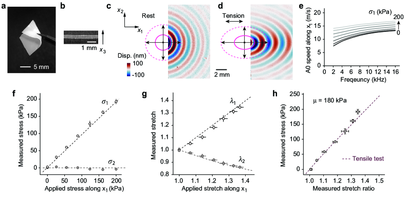
To validate the method, we devised an experimental setup (Supplementary Fig. S3) based on a home-built, swept-source OCT system [14]. The first sample used was a rubber sheet (Fig. 3a). We applied uniaxial tension to the sample using weights (see Methods). The thickness of the film measured by OCT (Fig. 3b) decreased from 500 to 430 m (Supplementary Fig. S4). Figures 3c,d show the wave profiles in the unstressed and fully stressed states (0 and 6 20-g weights, respectively) at = 6 kHz (see Supplementary Movies 1 and 2). In the unstressed state the wave propagates at the same speed in all directions, and creates a circular profile with . The applied stress, on the other hand, induces anisotropy for the speed, which creates an elliptical profile, with the speed along the tensile axis being larger than the speed along the compressive axis. Figure 3e shows the dispersion curves of the A0 mode at different stress levels from 0 to 200 kPa. We also measured the dispersion of the A0 wave along the axis (Supplementary Fig. S7).
The measured wave speeds and fit very well into the dispersion relation written in terms of (Supplementary Fig. S6), from which we determined and , and and . Using Eq. (1), we then obtained the stress and strain along the and axis. Figure 3f shows the measured and actual values of the two principal stresses with a good agreement, with errors around 5%. Figure 3g shows the measured and actual stretch ratios again in a good agreement with errors less than 3%. The measured stress-strain curve (Fig. 3h) gives a value of kPa, which agrees well with that obtained by an independent standard tensile test (Supplementary Fig. S8).
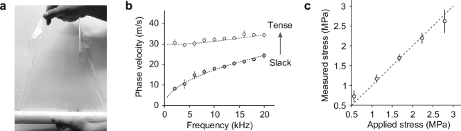
Next, we tested the technique for a stretched plastic wrap, a.k.a. cling film (Fig. 4a) made of polyethylene with a thickness of m. Using a similar experimental setup, we applied a uniaxial stress to the cling film and measured the dispersion relations at the unstressed and stressed states (Fig. 4b). For the ultra-thin structure, the asymptotic speed in the low frequency limit provides directly. We measured the low-frequency wave speed in the stretched condition to be m/s. Using = 930 kg/m3 we obtain MPa. By Taylor expansion of Eq. (2), we find , where is the Young’s modulus in the stretched condition. By curve fitting the measured dispersion curve (Fig. 4b), we find MPa. This is slightly lower than the Young’s modulus of MPa in the unstressed condition. Experiments performed at different stretching force showed good agreements between the measured and applied stress values (Fig. 4c).
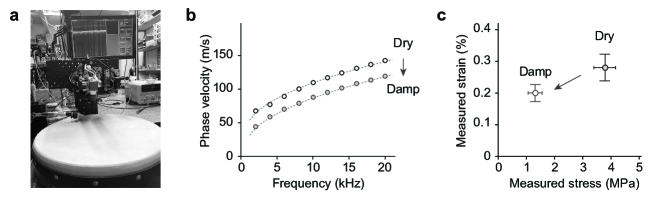
Finally we applied our technique to measure the stress in the drumhead of a musical instrument called the bodhrán drum, a traditional Irish drum made with goat skin. If the skin is too taut, the pitch is higher than expected, so players are advised to sprinkle and spread some water on the skin from the inside just before performance. Conversely, if the skin is too loose, bodhrán players rub their palm on the outside of the skin to make it dry and tighten the skin to correct the pitch.
The thickness of the skin was measured to be m. We performed in situ measurements on the drumhead (Fig. 5a) at normal (dry) and hydrated conditions of the skin. In the dry condition, the fundamental resonance frequency of the instrument was 84 Hz, and it was decreased to 36 Hz after hydration (Supplementary Fig. S9). The goat skin is intrinsically anisotropic, but our experiments revealed almost circular wave profiles (Supplementary Movies 3 and 4). This is well explained by the large radial stress in the drum, which stretches collagen fibres along the stress field [15]. The applied strain is transversely isotropic (equi-biaxial in the radial/circumferential directions) and thus, for all intends and purposes, acoustic wave propagation is isotropic in the drum plane. Figure 5b shows the dispersion relations of the skin in the dry and damp states, obtained at a region in the drum head. We determined from the experimental data that the amount of radial stretch in the dry skin is 0.28% and that humidification relaxed it to 0.20% (Fig. 5c). The corresponding stress is changed from 3.79 MPa (dry) to 1.31 MPa (damp). Noting that the strain is small, we find the Young’s modulus of the skin to be 680 MPa for dry skin and 330 MPa for the moisturized skin.
The result reveals how much the humidification changed the stiffness and consequently the tension of the skin. Hydration alters the resonance frequencies or pitch of the instrument, which is proportional to . The 65% reduction in tension (and an increase of density) predicts 46% decrease in resonance frequency. This is comparable to the actual 57% decrease of the resonance frequency. The discrepancy is probably due to spatially nonuniform hydration across the large drum head (18-inch diameter).
Discussion
The technique we present is nearly model-free in the sense that it is independent of and does not require the material’s mechanical properties. Although our method assumes the material is incompressible, extending the method to accommodate compressibility adds a relative small error in the order of , where is the first Lamé constant (Supplementary Note S2 and Fig. S2). The plastic cling film we tested is actually a compressible material with an initial Poisson’s ratio of and had significant plastic deformation. The technique is primarily for elastic materials, but it can be applied to weakly viscoelastic materials [16]. However, highly viscoelastic materials with frequency-dependent mechanical properties call for more involved curve fitting with parameters including the viscosity [17].
Although we have validated the technique for relatively uniform stress, it is easily applicable to more complex structures with spatially varying stress and strain fields by measuring local velocity profiles, as illustrated in Fig. 1c. The spatial resolution of the mapping is approximately in the order of one wavelength. When = 10 m/s, for example, the resolution is 5 mm for = 2-10 kHz. It is relatively straightforward to extend our method to thin structures in contact with fluids or gel-like matters either one side or both sides, such as dura mater of the brain after craniotomy [18] and the cornea [14] as well as blood vessel walls [19]. Our work is expected to pave the way to practical applications.
References
- [1] Gómez-González, M., Latorre, E., Arroyo, M. & Trepat, X. Measuring mechanical stress in living tissues. \JournalTitleNature Reviews Physics 2, 300–317, DOI: 10.1038/S42254-020-0184-6 (2020).
- [2] Schajer, G. S. Advances in hole-drilling residual stress measurements. \JournalTitleExperimental Mechanics 50, 159–168, DOI: 10.1007/S11340-009-9228-7 (2009).
- [3] Butt, H.-J., Graf, K. & Kappl, M. Physics and Chemistry of Interfaces (John Wiley & Sons, 2013).
- [4] Erbil, H. Y. et al. Surface Chemistry of Solid and Liquid Interfaces (Blackwell Pub. Oxford^ eMAMalden MA, 2006).
- [5] Aumaitre, E., Vella, D. & Cicuta, P. On the measurement of the surface pressure in Langmuir films with finite shear elasticity. \JournalTitleSoft Matter 7, 2530–2537, DOI: 10.1039/C0SM01213K (2011).
- [6] Shi, F., Michaels, J. E. & Lee, S. J. In situ estimation of applied biaxial loads with Lamb waves. \JournalTitleThe Journal of the Acoustical Society of America 133, 677, DOI: 10.1121/1.4773867 (2013).
- [7] Lanoy, M., Lemoult, F., Eddi, A. & Prada, C. Dirac cones and chiral selection of elastic waves in a soft strip. \JournalTitleProceedings of the National Academy of Sciences 117, 30186–30190, DOI: 10.1073/PNAS.2010812117 (2020).
- [8] Thelen, M., Bochud, N., Brinker, M., Prada, C. & Huber, P. Laser-excited elastic guided waves reveal the complex mechanics of nanoporous silicon. \JournalTitleNature Communications 12, 1–10, DOI: 10.1038/s41467-021-23398-0 (2021).
- [9] Hughes, D. S. & Kelly, J. L. Second-order elastic deformation of solids. \JournalTitlePhysical Review 92, 1145–1149, DOI: 10.1103/PhysRev.92.1145 (1953).
- [10] Ogden, R. W. Incremental statics and dynamics of pre-stressed elastic materials. In Destrade, M. & Saccomandi, G. (eds.) Waves in Nonlinear Pre-Stressed Materials, 1–26, DOI: 10.1007/978-3-211-73572-5_1 (Springer Vienna, Vienna, 2007).
- [11] Ogden, R. & Roxburgh, D. The effect of pre-stress on the vibration and stability of elastic plates. \JournalTitleInternational Journal of Engineering Science 31, 1611–1639, DOI: https://doi.org/10.1016/0020-7225(93)90079-A (1993).
- [12] Li, Guo-Yang, Gower, Artur L & Destrade, M. An ultrasonic method to measure stress without calibration: The angled shear wave method. \JournalTitleThe Journal of the Acoustical Society of America 127, 2759, DOI: https://doi.org/10.1121/10.0002959 (2020).
- [13] Destrade, M., Gilchrist, M. D. & Saccomandi, G. Third- and fourth-order constants of incompressible soft solids and the acousto-elastic effect. \JournalTitleJournal of the Acoustical Society of America 127, 2759, DOI: 10.1121/1.3372624 (2010).
- [14] Ramier, A., Tavakol, B. & Yun, S.-H. Measuring mechanical wave speed, dispersion, and viscoelastic modulus of the cornea using optical coherence elastography. \JournalTitleOptics Express 27, 16635–16649, DOI: 10.1364/OE.27.016635 (2019).
- [15] Deroy, C., Destrade, M., Mc Alinden, A. & Ní Annaidh, A. Non-invasive evaluation of skin tension lines with elastic waves. \JournalTitleSkin Research and Technology 23, 326–335, DOI: https://doi.org/10.1111/srt.12339 (2017). https://onlinelibrary.wiley.com/doi/pdf/10.1111/srt.12339.
- [16] Bercoff, J., Tanter, M. & Fink, M. Supersonic shear imaging: A new technique for soft tissue elasticity mapping. \JournalTitleIEEE Transactions on Ultrasonics, Ferroelectrics, and Frequency Control 51, 396–409, DOI: 10.1109/TUFFC.2004.1295425 (2004).
- [17] de Rooij, R. & Kuhl, E. Constitutive modeling of brain tissue: Current perspectives. \JournalTitleApplied Mechanics Reviews 68, DOI: 10.1115/1.4032436 (2016).
- [18] Hartmann, K., Stein, K. P., Neyazi, B. & Sandalcioglu, I. E. Optical coherence tomography of cranial dura mater: Microstructural visualization in vivo. \JournalTitleClinical Neurology and Neurosurgery 200, 106370, DOI: 10.1016/J.CLINEURO.2020.106370 (2021).
- [19] Li, G.-Y. et al. Guided waves in pre-stressed hyperelastic plates and tubes: Application to the ultrasound elastography of thin-walled soft materials. \JournalTitleJournal of the Mechanics and Physics of Solids 102, DOI: 10.1016/j.jmps.2017.02.008 (2017).
- [20] Scarcelli, G. et al. Noncontact three-dimensional mapping of intracellular hydromechanical properties by Brillouin microscopy. \JournalTitleNature Methods 12, 1132–1134, DOI: 10.1038/nmeth.3616 (2015).
Methods
Theoretical model
We consider an elastic wave polarised in the plane, propagating along the axis ( or ), with attenuation along the axis: . Inserting into and eliminating with the incompressibility , we get the secular equation
| (3) |
where , , and . With the stress-free boundary condition at , we arrive at the dispersion equation for the Lamb wave [11]
| (4) |
where the exponent is for symmetric modes and for anti-symmetric modes, and , are the roots of Eq. (3).
To capture the acousto-elastic effect induced by a moderate strain, we consider the strain energy of isotropic incompressible third-order elasticity [12, 13]. The elastic moduli are given by Equation (9) in Li et al [12], which result in . Substituting into Eq. (3) we get and , and the dispersion equation Eq. (4) becomes Eq. (2).
The basic idea of our acousto-elastic imaging technique is to deduce the stress and strain with and from the exact formulas
| (5) |
To show these formulas, it suffices to recall that, in general [10],
| (6) |
Making use of Eq. (6), we get , and , which leads to Eq. (5) by taking (thin membrane).
Expanding (4) in the low frequency limit of (or ), we get and for the A0 and S0 modes, respectively. On the other hand, in the high frequency limit of (or ), we get for both A0 and S0 modes, where is the real root of the cubic (Rayleigh surface wave limit). The three limits are shown in Fig. 2d.
As a simple example, suppose an initially isotropic material is subject to a small stress. In the limit of small deformation (, using Taylor expansion the three limits can be explicitly expressed as functions of the principal stresses
| (7) |
For thin structures, . If two of these three limiting wave speeds are measured, the in-plane stresses () can be calculated from this equation with . In practice, the limit cannot be measured accurately because it corresponds to an extremely thick slab. Similarly it is difficult to express the mode for ultra-thin films; in that case, the first equation for the mode nonetheless gives access to directly.
Experimental setup
Our experimental setup (Supplementary Fig. S3) is based on a home-built, swept-source optical coherence tomography (OCT) system [14]. This system offers an A-line rate of 43.2 kHz, axial resolution of m (in the air) and transverse resolution of m, using a polygon swept laser with a tuning range of 80 nm and a centre wavelength of 1,280 nm. The optical beam is scanned using a two-axis galvanometer scanner. To excite Lamb waves in the film we used a contact probe driven by a vibrating PZT piezoelectric transducer (Thorlabs, PA4CEW). The plastic probe was 3D-printed with a spherical tip of mm in diameter. A small force ( mN) was applied to the probe to keep it in contact with the sample. The optical beam scan was synchronized with the probe vibration to operate in an M-B scan mode (see Supplementary Note 3 and Fig. S10). Their scanner axes were aligned to the principal transverse axes (). The frequency of the vibration was step-tuned from 2 to 20 kHz with an interval of 2 kHz. At each frequency, the amplitudes and phases of the vibrations were acquired at 96 transverse locations. The vertical displacement near the probe contact point at the sample was in the order of 100 nm in the frequency range. To measure this small vibration, we used the phase change in the interference signal of the OCT [14].
To measure the wavenumber and thus the wave speed for a given frequency, the surface displacement was Fourier-transformed from the spatial domain to the wavenumber domain. The wavenumber was obtained by identifying the peak that corresponds to the A0 mode (Supplementary Fig. S5). The standard deviation error in the wavenumber measurement is estimated to be about (Supplementary Note 4).
For the experiments of the rubber sheet and cling film, the sample was clamped along its two short edges and one clamp was pulled horizontally by a cord connected to 1 to 6 weights (20 g each) to apply a uniaxial tension with varying magnitudes. The Cauchy stress applied to the film is , where and are the initial width and half-thickness of the sample, respectively, m/s2 is the acceleration of gravity and is the number of the weights. When changing the stress state, the results obtained during loading and unloading were averaged to minimise the effect of hysteresis.
For each stress state, the current thickness of the rubber film was measured from the OCT image. The uniaxial stretch ratio was then determined by . The measured stretch ratio agreed well with that obtained by the deformation of the grids drew on the surface of the rubber film.
Materials
The rubber sheet has mass density 1,070 kg/m3 and refractive index . The initial dimension was mm, mm, and mm. The lateral size was large enough to avoid wave reflections at the edges. The rubber sample was prepared from Ecoflex 5 material (Smooth-On Inc) by mixing the Ecoflex 1A and 1B at 1:1 ratio by weight. The mixture was poured into a mold and cured at room temperature overnight. Then the material was post-cured in an oven at 80∘C for 2 hours. For mechanical testing, we cut out a small piece ( mm3) and performed a tensile test with a uniaxial tensile testing machine (eXpert 4000 Micro Tester, Admet, Norwood, USA). Figure 3e shows the resulting stress-stretch curve. Applying a linear fitting to the initial stage of the curve (stretch ratio < 1.07) we find that the initial shear modulus (one third of the Young modulus) is approximately 180 kPa.
We used a common home-use cling film (plastic wrap) made of polyethylene with kg/m3. The typical thickness of cling films ranges from 8 to 13 m. Here we used Brillouin microscopy [20] to measure the thickness of our film to be m. This is close to the axial resolution of the OCT system, and so we could not track with the deformation.
The bodhrán instrument was purchased from Hobgoblin Music, MN, USA. The OCT measurement was performed on the intact instrument. On separate direct measurements after removing the skin from the frame, we found m and kg/m3 in the dry condition. After hydration, the density is expected to increase to 1000 kg/m3. To characterise the fundamental resonance frequencies of the instrument in the dry and damp conditions, the centre of the drumhead was beaten every 10 seconds while recording the sound with a cellphone 10 cm away from the drumhead, using the Google Science Journal App.
Acknowledgements
This study was supported by grants P41-EB015903, R01-EB027653, DP1-EB024242 from the National Institutes of Health (USA) for G.Y.L and S.H.Y, and by the 111 Project for International Collaboration No. B21034 (Chinese Government, PR China), a grant from the Seagull Program (Zhejiang Province, PR China) for M.D and a grant from the European Commission - Horizon 2020 / H2020 - Shift2Rail for A.L.G. The authors thank Drs Amira Eltony and Xu Feng for help with the measurements, and Pasquale Ciarletta, Niall Colgan and Giuseppe Zurlo for valuable feedback.
Author contributions statement
G.Y.L., A.G., and M.D. designed the study. G.Y.L., A.G., and M.D. developed the theoretical model. G.Y.L. conducted the experiments. G.Y.L. and S.H.Y. analyzed the results. All authors wrote and reviewed the manuscript.