Cyber-Physical-Systems and Secrecy Outage Probability: Revisited

Abstract

This paper technically explores the secrecy rate $\Lambda$ and a maximisation problem over the concave version of the secrecy outage probability (SOP) as $\mathop{{\rm\mathbb{M}ax}}\limits_{\Delta}{\rm\;}\mathbb{P}\mathscr{r}\big{(}\Lambda\geq\lambda\big{)}$. We do this from a generic viewpoint even though we use a traditional Wyner’s wiretap channel for our system model $-$ something that can be extended to every kind of secrecy modeling and analysis. We consider a Riemannian mani-fold for it and we mathematically define a volume for it as $\mathbb{V}\mathscr{ol}\big{\{}\Lambda\big{\}}$. Through achieving a new bound for the Riemannian mani-fold and its volume, we subsequently relate it to the number of eigen-values existing in the relative probabilistic closure. We prove in-between some novel lemmas with the aid of some useful inequalities such as the Finsler’s lemma, the generalised Young’s inequality, the generalised Brunn-Minkowski inequality, the Talagrand’s concentration inequality. We additionally propose a novel Markov decision process based reinforcement learning algorithm in order to find the optimal policy in relation to the eigenvalue distributions $-$ something that is extended to a possibilisitically semi-Markov decision process for the case of periodic attacks.

I Introduction

Physical-layer security inevitably plays a vital role in 5/6 G and beyond. This widely supported concept [1, 2, 3, 4, 5, 6, 7, 8, 9, 10, 11, 12] is emerged in parallel with traditional cryptography techniques while information-theoretic perspectives are promising.

In order to simultaneously enhance the fairness and the quality of service among all the users, the physical characteristics of the wireless channel are of an absolutely inconsistent nature, which originally comes from the channel’s broadcast behaviour $-$ something that should be essentially managed.

The concept of secrecy outage probability (SOP) in telecommunication still shows up an open research field in the literature. This concept is useful e.g. for: free-space optical communications [1], vehicular communications [2], reflecting intelligent surfaces [3]-[4], cognitive networks [5], cooperative communications [6], power-line communications [7], the internet of Things [8], terrestrial networks [9], mobile edge computing networks [10], molecular communications [11] and under-water networks [12].

In [1]-[12] and in totally various types of system models, some novel and closed-form mathematical expressions have been newly derived and proposed $-$ some of them are optimisation based, some of them are statistical oriented and some of them are even jointly theoretical-practical.

I-A Motivations and contributions

In this paper, we are interested in responding to the following question: How can we guarantee highly adequate relaxations over the principle of SOP? With regard to the non-complete version of the literature, the expressed question strongly motivate us to find an interesting solution, according to which our contributions are fundamentally described as follows.

• (i) A new bound in relation to the maximisation problem over the SOP’s concave version is derived. We, in addition, theoretically discuss about a totally novel interpretation over the aforementioned maximisation problem from a duality point of view. We consider a Riemannian mani-fold for the SOP’s concave version and we mathematically define a volume for it for which we derive a new bound. We use some insightful principles such as Keyhole contour.

• (ii) We subsequently relate the Riemannian mani-fold and its bounded volume expressed above to the number of eigen-values. We use in-between some useful lemmas and inequalities such as the Finsler’s lemma, the generalised Young’s inequality, the generalised Brunn-Minkowski inequality, the Talagrand’s concentration inequality.

• (iii) We additionally go over further discussions in terms of the projection method technically relating it to the former parts. We also take into account the case of relaxing the non-contractibility and how to decrease the relative non-contractibility radius from a topological point of view. In this context, we propose a novel Markov decision process based reinforcement learning algorithm in order to find the optimal policy in relation to the eigenvalue distributions $-$ something that was subsequently extended to a semi-Markov decision one for the case of periodic attacks and with regard to the possibility-theory.

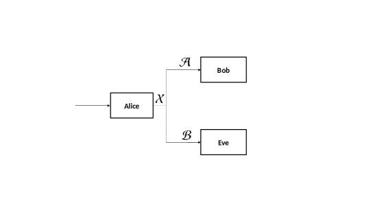
(a)

Figure 1: A traditional Wyner’s wiretap channel: System diagram of a communication which suffers from insecurity while $\mathcal{X}$, $\mathcal{A}$ and $\mathcal{B}$ are random states relating to respectively Alice, Bob and Eve.

I-B General notation

The notations widely used throughout the paper is given in Table I.

TABLE I: List of notations.

Notation	Definition	Notation	Definition
$\mathbb{M}in$	Minimisation	$\mathbb{M}ax$	Maximisation
$\mathbb{E}$	Expected-value	$\mathcal{I}(\cdot)$	Mutual-information
$\stackrel{{\scriptstyle def}}{{=}}$	Is defined as	$\approx$	Is approximated to
$\mathbb{V}\mathscr{ol}$	Volume	$\mathbb{P}\mathscr{r}$	Probability
$det(\cdot)$	Matrix determinant	$(\cdot)^{T}$	Transpose
$Tr[\cdot]$	Trace of matrix	$(\cdot)^{-1}$	Inverse of matrix
$\Lambda$	Secrecy rate	$\mathbb{P}\mathscr{r}\big{(}\Lambda\geq\lambda\big{)}$	SOP’s Concave Version
$\mathscr{t}$	Time	$\mathscr{H}$	Entropy
$\mathcal{M}$	Riemannian-manifold	$\partial\mathcal{M}$	Boundary
$\zeta$	Eigen-value	$Tr[\cdot]$	Trace

I-C Organisation

The rest of the paper is organised as follows. The system set-up and our main results are given in Sections II and III. Subsequently, the evaluation of the framework and conclusions are given in Sections IV and V. In Fig. 2, the flow of the main problem and the solution to that is deppicted.

II System model and problem formulation

In this section, we describe the system model, subsequently, we formulate the basis of our problem.

II-A System description: A traditional Wyner’s wiretap channel $-$ without loss of generality

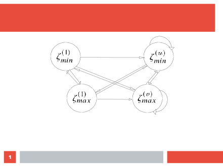
(a)

Figure 4: The Markov model in relation to our scheme and $\big{\{}\zeta^{(1)}_{max},\cdots,\zeta^{(\mathscr{v})}_{max}\big{\}}$ as well as the $\big{\{}\zeta^{(1)}_{min},\cdots,\zeta^{(\mathscr{u})}_{min}\big{\}}$ .

A traditional Wyner’s wiretap channel based communication scenario includes a transmitter named Alice and a legitimate reciever named Bob and an un-authorised one as an eavesdropper named Eve, as shown in Fig. 4. The information capacity of the communication system is theoretically expressed by the general formula from Shannon. The secrecy capacity is interpreted as a bound of the security performance of the communication system. We now have the following inequality for the secrecy capacity from an information-theoretic point of view

$$\begin{split}\;C_{s}\stackrel{{\scriptstyle def}}{{=}}\mathop{{\rm\mathbb{M}ax}}\limits_{f_{\mathcal{X}}(x)}{\rm\;}\mathcal{I}\big{(}\mathcal{X},\mathcal{A}\big{)}-\mathcal{I}\big{(}\mathcal{X},\mathcal{B}\big{)}\;\;\;\;\;\;\;\;\;\\ \geq\mathop{{\rm\mathbb{M}ax}}\limits_{f_{\mathcal{X}}(x)}{\rm\;}\mathcal{I}\big{(}\mathcal{X},\mathcal{A}\big{)}-\mathop{{\rm\mathbb{M}ax}}\limits_{f_{\mathcal{X}}(x)}{\rm\;}\mathcal{I}\big{(}\mathcal{X},\mathcal{B}\big{)},\end{split}$$ (1)

while $\mathcal{X}$, $\mathcal{A}$ and $\mathcal{B}$ are random states relating to respectively Alice, Bob and Eve, where the maximisation takes place over the encoding function $f_{\mathcal{X}}(x)$ $-$ and consequently input distributions $-$ , that is, $f_{\mathcal{X}}(x)$ $-$ the input distributions $-$ should be optimally found by Alice in the sense that the overall performance can be technically guaranteed with regard to the metric of the secrecy capacity $C_{s}$. Hereinafter, we r-call $C_{s}$ as $\Lambda$.

II-B Main problem

The main problem w.r.t. the secrecy rate $\Lambda$ is about the maximisation problem over the SOP’s concave version $\mathbb{P}\mathscr{r}\big{(}\Lambda\geq\lambda\big{)}$, that is, $\mathop{{\rm\mathbb{M}ax}}\limits_{\Delta=\big{\{}\lambda_{1},\cdots,\lambda_{n}\big{\}}}{\rm\;}\mathbb{P}\mathscr{r}\big{(}\Lambda\geq\lambda\big{)}$ where the parameters are defined in the next section. Furthermore, we discuss how to reach out the relative eigen-values.

Assumption 1. We consider that the dynamical system

$$\begin{split}\;\mathcal{X}^{(t+1)}=a_{1}\mathcal{X}^{(t)}+\mathscr{w}_{0}^{(t+1)},\;\;\;\;\;\;\;\;\;\;\;\;\;\;\;\;\;\;\;\;\;\;\;\;\;\;\\ \big{(}\mathcal{A}^{(t)},\mathcal{B}^{(t)}\big{)}=\big{(}a_{2},a_{3},\big{)}\mathcal{X}^{(t)}+\big{(}\mathscr{w}_{1}^{(t)},\mathscr{w}_{2}^{(t)}\big{)},\end{split}$$ (2)

is satisfied while $(a_{1},a_{2},a_{3})$ and $(\mathscr{w}_{0},\mathscr{w}_{1},\mathscr{w}_{3})$ are respectively the control parameter tuple and the noise one. is unstable, that is, its spectral radius is

$$\begin{split}\;\varphi(a_{1})=\mathop{{\rm\mathbb{M}ax}}\limits_{i}{\rm\;}|\zeta(a_{1})|>1,\end{split}$$ (3)

is satisfied.

III Main results

In this section, our main results are theoretically provided in details.

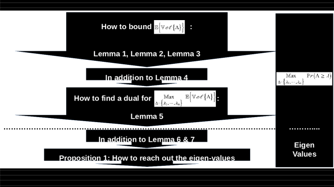
(a)

Figure 2: Flow of problem-and-solution.

Definition 1. Let us theoretically assign a random variable $\Lambda(\mathscr{t})\stackrel{{\scriptstyle def}}{{=}}\big{\{}\lambda_{1},\cdots,\lambda_{n}\big{\}}$ for the secrecy rate according to which the SOP’s concave version can be defined as $\mathbb{P}\mathscr{r}\big{(}\Lambda\geq\lambda\big{)}$ as well.

Lemma 1

For the random variable $\Lambda(\mathscr{t})\stackrel{{\scriptstyle def}}{{=}}\big{\{}\lambda_{1}(\mathscr{t}),\cdots,\lambda_{n}(\mathscr{t})\big{\}}$ over the time horizon $-$ for which the term $(\mathscr{t})$ is neglected hereinafter for the ease of notation $-$, the expression

$$\begin{split}\;\mathbb{E}\big{\{}\Lambda\big{\}}\leq\frac{\mathbb{E}\big{\{}e^{\mathscr{t}\Lambda}\big{\}}-1}{\mathscr{t}},\end{split}$$ (4)

is satisfied.

Proof: The proof is convenient to follow according to the Taylor-expansion theorem, however, see Appendix A for more detailed justifications.$\;\;\;\blacksquare$

In the following, roughly speaking, we consider the secrecy rate as a Riemannian mani-fold for which a volume is technically defined.

Remark 1: The reason why we consider a vloume can be theoretically justified as follows. Unhesitatingly, since we consider the relative parameters as Riemannian mani-folds, one can justify a volume over them from a generic point of view. In particular and as obvious e.g. from [15, 16] and in the context of the Asymptotic Equipartition Property, one can interpret the volume of a random variable $-$ only for the secrecy rate $\Lambda$ but not the SOP’s concave version $\mathbb{P}\mathscr{r}\big{(}\Lambda\geq\lambda\big{)}$ $-$ as the exponential of Shannon’s entropy of it. Indeed, this property can be elaborated via the Cramer’s large deviation theorem. Meanwhile, in relation to the volume of the random variable, please do not misunderstand it with the standard deviation as we are generalising it.

Definition 2. Let us, for more generalisations, consider the secrecy rate as the Riemannian mani-fold $\mathcal{M}$ for which the volume $\mathbb{V}\mathscr{ol}\big{\{}\Lambda\big{\}}$ is valid. Undoubtedly, $\mathcal{M}$ can be contractible if its Euler characteristics gets $\mathscr{X}(\mathcal{M})=1$, that is, if $\mathcal{M}$ is homotopically equivalent to a single-point, that is, when and if $\mathcal{M}$ is continously shrunk and topologically deformed into a sigle-point. In other words, a space is contractible iff the identity map from it to itself $-$ which is always a homotopy equivalence $-$ is null-homotopic [17, 18, 19, 20].

In order to further justify Definition 2, re-call Assumption 1. Indeed, when a system is unstable, the more uncertainty is amplified originating from the noise. Thus, Eve cannot always predict the system close to an equilibrium [21]. Or in other words, if: (i) $(a_{1},a_{2})$ is observable; and (ii) $(a_{1},\sqrt{a_{2}})$ is controllable, the error covariance matrix at Eve converges exponentionally to a unique fixed-point [22]. We have consequently to consider inverse.

Definition 3 $-$ Tangent Cone. The term tangent cone is defined as $\omega_{\mathcal{M}}(x)\stackrel{{\scriptstyle def}}{{=}}\lim_{h\to 0}inf\frac{dist\big{(}x+h\omega,\mathcal{M}\big{)}}{h}=0$ while $dist(\cdot,\cdot)$ stands literally for the information theoretic distance(s).

Definition 4 $-$ Inward-pointing. If $f(\cdot)$ is a vector-field relating to $\mathcal{M}$ and the boundary $\partial\mathcal{M}$ exists, $f(\cdot)$ is said to be oint inward to $\mathcal{M}$ at a point $x\in\mathcal{M}$ if $f(x)\in\omega_{\mathcal{M}}(x)-\big{\{}\omega_{\partial\mathcal{M}}(x)\big{\}}$ holds.

Corollary 1. Any compact and convex set is contractible, but not vise versa. Meamwhile, every contractible set, even non-convex, has a concave volume. Finally, every vector field that is inward-point to $\mathcal{M}$ has an equilibrium [27, 28] as there exists at least one contractible interior within the boundary $\partial\mathcal{M}$, if $\partial\mathcal{M}$ exists.

Objective. Our aim is to increase the contractibility radius as much as possible.

III-A How to define a maximisation problem over the SOP’s concave version as $\mathop{{\rm\mathbb{M}ax}}\limits_{\Delta=\big{\{}\lambda_{1},\cdots,\lambda_{n}\big{\}}}{\rm\;}\mathbb{P}\mathscr{r}\big{(}\Lambda\geq\lambda\big{)}$ w.r.t. the secrecy rate $\Lambda$

Lemma 2

Vitale’s random Brunn-Minkowski inequality $-$ The expression

$$\begin{split}\;\mathbb{V}\mathscr{ol}\Big{\{}\mathbb{E}\big{\{}\Lambda\big{\}}\Big{\}}\geq\mathbb{E}\Big{\{}\mathbb{V}\mathscr{ol}\big{\{}\Lambda\big{\}}\Big{\}},\end{split}$$ (5)

holds.

Lemma 3

The expression

$$\begin{split}\;\mathbb{V}\mathscr{ol}\Big{\{}\frac{\mathbb{E}\big{\{}e^{\mathscr{t}\Lambda}\big{\}}-1}{\mathscr{t}}\Big{\}}\geq\mathbb{E}\Big{\{}\mathbb{V}\mathscr{ol}\big{\{}\Lambda\big{\}}\Big{\}},\end{split}$$ (6)

holds.

Proof: The proof is easy to follow by an integration of Lemma 1 and Lemma 2. This is due to the fact that $\mathbb{E}\Big{\{}\mathbb{V}\mathscr{ol}\big{\{}\Lambda\big{\}}\Big{\}}\leq\mathbb{V}\mathscr{ol}\Big{\{}\underbrace{\mathbb{E}\big{\{}\Lambda\big{\}}}_{\leq\frac{\mathbb{E}\big{\{}e^{\mathscr{t}\Lambda}\big{\}}-1}{\mathscr{t}}}\Big{\}}$ holds.$\;\;\;\blacksquare$

Lemma 4

The expression

$$\begin{split}\;\mathbb{E}\big{\{}e^{\mathscr{t}\Lambda}\big{\}}=e^{\mathscr{t}\lambda}\mathbb{P}\mathscr{r}\big{(}\Lambda\geq\lambda\big{)},\end{split}$$ (7)

strongly holds.

Proof: See Appendix B.$\;\;\;\blacksquare$

Lemma 5

The problem

$$\begin{split}\;\mathop{{\rm\mathbb{M}ax}}\limits_{\Delta=\big{\{}\lambda_{1},\cdots,\lambda_{n}\big{\}}}{\rm\;}\mathbb{V}\mathscr{ol}\Big{\{}e^{\mathscr{t}\lambda}\Big{\}}\mathbb{V}\mathscr{ol}\Big{\{}\mathbb{P}\mathscr{r}\big{(}\Lambda\geq\lambda\big{)}\Big{\}},\end{split}$$ (8)

can be a dual one for the problem

$$\begin{split}\;\mathop{{\rm\mathbb{M}ax}}\limits_{\Delta=\big{\{}\lambda_{1},\cdots,\lambda_{n}\big{\}}}{\rm\;}\mathbb{E}\Big{\{}\mathbb{V}\mathscr{ol}\big{\{}\Lambda\big{\}}\Big{\}}.\end{split}$$ (9)

Proof: See Appendix C.$\;\;\;\blacksquare$

Algorithm 1 A greedy algorithm to $\Lambda$.

  Initialisation. while $\mathbb{TRUE}$ do           Find the solution to $\Delta\in\Bigg{\{}\mathop{{\rm\mathbb{M}ax}}\limits_{\Delta=\big{\{}\lambda_{1},\cdots,\lambda_{n}\big{\}}}{\rm\;}\mathbb{E}\Big{\{}\mathbb{V}\mathscr{ol}\big{\{}\Lambda\big{\}}\Big{\}},\mathop{{\rm\mathbb{M}ax}}\limits_{\Delta=\big{\{}\lambda_{1},\cdots,\lambda_{n}\big{\}}}{\rm\;}\mathbb{V}\mathscr{ol}\Big{\{}\mathbb{P}\mathscr{r}\big{(}\Lambda\geq\lambda\big{)}\Big{\}}\Bigg{\}}$. endwhile end Output: $\Lambda$

Remark 2:

• (i) $\mathbb{V}\mathscr{ol}\Big{\{}e^{\mathscr{t}\lambda}\Big{\}}.$ Whether $\mathop{{\rm\mathbb{M}ax}}\limits_{\Delta=\big{\{}\lambda_{1},\cdots,\lambda_{n}\big{\}}}{\rm\;}\mathbb{V}\mathscr{ol}\Big{\{}e^{\mathscr{t}\lambda}\Big{\}}$ is of a partially useless nature here for our main problem or not, we use it as a trick which is of a purely useful nature in the next lemma.

• (ii) $\mathbb{V}\mathscr{ol}\Big{\{}\mathbb{P}\mathscr{r}\big{(}\Lambda\geq\lambda\big{)}\Big{\}}$. First of all, we have nothing to do with its maximum version, i.e., $1$. Additionally, recalling Definition 2 as well as Remark 1 in connection with $\mathbb{V}\mathscr{ol}\big{\{}\cdot\big{\}}$, we see that the aforementioned value is not by-default equated with $1$.

• (iii) Recaptulation. So far, we have indeed recasted the problem $\mathop{{\rm\mathbb{M}ax}}\limits_{\Delta=\big{\{}\lambda_{1},\cdots,\lambda_{n}\big{\}}}{\rm\;}\mathbb{P}\mathscr{r}\big{(}\Lambda\geq\lambda\big{)}$ into two parts, i.e., $\mathop{{\rm\mathbb{M}ax}}\limits_{\Delta=\big{\{}\lambda_{1},\cdots,\lambda_{n}\big{\}}}{\rm\;}\mathbb{V}\mathscr{ol}\Big{\{}e^{\mathscr{t}\lambda}\Big{\}}$ and $\mathop{{\rm\mathbb{M}ax}}\limits_{\Delta=\big{\{}\lambda_{1},\cdots,\lambda_{n}\big{\}}}{\rm\;}\mathbb{V}\mathscr{ol}\Big{\{}\mathbb{P}\mathscr{r}\big{(}\Lambda\geq\lambda\big{)}\Big{\}}$ which are deterministic ones.

Lemma 6

The problem

$$\begin{split}\;\mathop{{\rm\mathbb{M}ax}}\limits_{\Delta=\big{\{}\lambda_{1},\cdots,\lambda_{n}\big{\}}}{\rm\;}\int\mathbb{V}\mathscr{ol}\Big{\{}e^{\mathscr{t}\lambda}\Big{\}}+\int\mathbb{V}\mathscr{ol}\Big{\{}\mathbb{P}\mathscr{r}\big{(}\Lambda\geq\lambda\big{)}\Big{\}},\end{split}$$ (10)

can be a dual for the problem

$$\begin{split}\;\mathop{{\rm\mathbb{M}ax}}\limits_{\Delta=\big{\{}\lambda_{1},\cdots,\lambda_{n}\big{\}}}{\rm\;}\mathbb{V}\mathscr{ol}\Big{\{}e^{\mathscr{t}\lambda}\Big{\}}\mathbb{V}\mathscr{ol}\Big{\{}\mathbb{P}\mathscr{r}\big{(}\Lambda\geq\lambda\big{)}\Big{\}},\end{split}$$ (11)

as its bound.

Proof: The proof is easy to follow with the aid of the generalised Yong’s ineqality which says that

$$\begin{split}\;f^{\prime}(x)g^{\prime}(x)\leq f(x)+g(x),\end{split}$$ (12)

holds for the arbitary functions $f(\cdot)$ and $g(\cdot)$, while $(\cdot)^{\prime}$ stands for the drivative.$\;\;\;\blacksquare$

III-B How to reach out the eigen-values

Remark 3: Regarding to the fact that mainly most of the secrecy rate problems can be discussed in the context of semi-definite algebra [4]-[12], that is the format $\mathcal{B}^{T}\mathcal{A}\mathcal{B}$, we jump in terms of the following to the next steps.

Lemma 7

Finsler’s lemma $-$ The problem

$$\begin{split}\;\exists\mathcal{X},\mathcal{X}^{T}\mathcal{A}\mathcal{X}=\xi,\mathcal{X}^{T}\mathcal{B}\mathcal{X}\leq\xi\Longrightarrow\exists z:\mathcal{B}-z\mathcal{A}<\xi,\end{split}$$ (13)

holds for the arbitary matrices $\mathcal{A}$ and $\mathcal{B}$ while $\xi$ and $T$ stand respectively for an arbitary threshold and the transpose operand.

Proposition 1

Let us assume the descriptor system $\big{(}\mathcal{B},\mathcal{A}\big{)}$, so, the characteristic polynomial is given as

$$\begin{split}\;\mathscr{P}(z)=det\big{(}\mathcal{B}-z\mathcal{A}\big{)},\end{split}$$ (14)

while $det(\cdot)$ stands for the matrix determinant. The number of eigenvalues in the region associated with the polynomial $\mathscr{P}(z)$ over the Riemannian $\mathbb{V}\mathscr{ol}\Big{\{}\mathbb{P}\mathscr{r}\big{(}\Lambda\geq\lambda\big{)}\Big{\}}$ is related to $\big{(}\mathcal{B}-z\mathcal{A}\big{)}^{-1}$ and $det\big{(}\mathcal{B}-z\mathcal{A}\big{)}$ while $(\cdot)^{-1}$ stands for the inverse matrix.

Proof: See Appendix D.$\;\;\;\blacksquare$

III-C Futher discussion

Proposition 2

Let the random $k-$dimensional subspace $\mathbb{P}\mathscr{r}\big{\{}\Lambda\geq\lambda\big{\}}$ be valid and let $v^{\prime}_{i}$ be the projection of the point $v_{i}\in\Lambda$ into $\mathbb{P}\mathscr{r}\big{\{}\Lambda\geq\lambda\big{\}}$. Now, calling $L=||v^{\prime}_{i}-v^{\prime}_{j}||^{2}$ and $\tau_{1}=k||v_{i}-v_{j}||^{2}$. The value of $\mathbb{P}\mathscr{r}\big{(}L\leq(1-\tau_{2})\tau_{1}\big{)}$ is bounded from above by $\leq exp\big{(}-\frac{k\tau^{2}_{2}}{4}\big{)},\forall\;0<k<\infty$.

Proof: See Appendix E.$\;\;\;\blacksquare$

Proposition 3

Consider $\Theta\in\mathbb{R}^{r\times m}$ and $\theta\in\mathbb{R}^{r\times m}$. The element-wise projection operator $Proj(\cdot):\in\mathbb{R}\times\mathbb{R}\rightarrow\mathbb{R}$ which is a convex and continuously differentiable function is defined as [41]

$$\begin{split}\;Proj(\theta_{ij},\Theta_{ij})=\;\;\;\;\;\;\;\;\;\;\;\;\;\;\;\;\;\;\;\;\;\;\;\;\;\;\;\;\;\;\;\;\;\;\;\;\;\;\;\;\;\;\;\;\;\;\;\;\;\;\;\;\;\;\;\;\;\;\;\;\;\\ \begin{cases}\Theta_{ij}-\Theta_{ij}f(\theta_{ij}),\;if\;f(\theta_{ij})>0\;\&\;\Theta_{ij}(\frac{df(\theta_{ij})}{d\theta_{ij}})>0,\\ \Theta_{ij},o.w.,\end{cases}\end{split}$$ (15)

where the index $(\cdot)_{ij}$ refers to the element in the $i^{th}$ row and the $j^{th}$ column and the convex and continuously differentiable function $f(\theta_{ij})$ is defined as

$$\begin{split}\;f(\theta_{ij})=\frac{(\theta_{ij}-\theta^{min}_{ij}-\eta_{ij})(\theta_{ij}-\theta^{max}_{ij}+\eta_{ij})}{(\theta^{max}\eta_{ij}-\theta^{min}_{ij}-\eta_{ij})\eta_{ij}},\end{split}$$ (16)

where $\eta_{ij}\in\mathbb{R}^{+}$ is the projection tolerance of $\theta_{ij}$ while $\eta_{ij}<\frac{\theta^{max}_{ij}-\theta^{min}_{ij}}{2}$ and $\eta_{ij}<\theta^{max}_{ij}\;\&\;|\theta^{min}_{ij}|$ hold, and while $\theta^{max}_{ij}>0$ and $\theta^{min}_{ij}<0$ are respectively the upper-bound and the lower-bound of $\theta_{ij}$. Now $Proj(\theta_{ij},\Theta_{ij})$ is a calculable function of our eigen-values discussed in the previous parts, that is, $\mathbb{P}\mathscr{r}\big{\{}\Lambda\geq\lambda\big{\}}$.

Proof: See Appendix F.$\;\;\;\blacksquare$

Proposition 4

Even if the secrecy rate $\Lambda$ is not convex and compact, or for more generality, it is not contractible, that can still be relaxed and an equilibrium can be consequently found in relation to the eigenvalues discussed above.

Proof: See Appendix G.$\;\;\;\blacksquare$

Proposition 5

For the case of periodic attacks, an extension over our Markov decision process and with regard to the possibility-theory is satisfied in term of a possibilisitically semi-Markov decision process.

Proof: See Appendix H.$\;\;\;\blacksquare$

IV Numerical results

Initially opening, we have done our simulations w.r.t. the Bernoulli-distributed data-sets using GNU Octave of version $4.2.2$ on Ubuntu $16.04$.

Consider a three-dimensional coordinate network setup consisting of Alice located at $(-50,0,0)$, Bob located at $(0,50\sqrt{3},0)$ and Eve located at $(0,-d,0)$ while $d$ is given unkown. Indeed, the distance between Alice and Bob is $D_{AB}=100\;m$ and the distance between Alice and Eve is $D_{AE}=\sqrt{50^{2}+d^{2}}\;m$. The channel matrices are modeled as $H=D_{AB}^{-\epsilon/2}\hat{H}$ and $G=D_{AE}^{-\epsilon/2}\hat{G}$ for respectively Alice-Bob link and Alice-Eve one while $\hat{H}$ and $\hat{G}$ are small-scale Rayleigh fading modeled matrices with i.i.d. complex Gaussian entries with the zero-mean and the variance of $\frac{1}{size}$ where $size$ is the size of the relative matrices, and $\epsilon$ stands for the path-loss exponent $-$ something that is chosen $3$. Consequently, the signal-to-noise-ratio (SNR) values at Bob and Eve are respectively deriven as $SNR_{B}=\frac{P_{a}}{D_{AB}^{\epsilon}\partial^{2}_{b}}$ and $SNR_{E}=\frac{P_{a}}{D_{AE}^{\epsilon}\partial^{2}_{e}}$ where $P_{a}$ stands literally for the transmition power of Alice, while $\partial^{2}_{b}$ and $\partial^{2}_{e}$ are the noise variances at Bob and Eve, respectively.

Table II shows the SOP’s convex version vs. $\mathcal{I}\big{(}\mathcal{X},\mathcal{A}\big{)}$ while changing $\rho$ $-$ something that is perfect for the evaluation here. We indeed use $\frac{e^{-\rho^{2}}}{\mathbb{P}\mathscr{r}\big{(}\Lambda\big{)}}$, something that can be in connection with another lower-bound from a traditional point of view, that is, $\mathbb{P}\mathscr{r}\big{(}\frac{SNR_{B}}{SNR_{E}}<2^{R_{s}}\big{)}$ while $R_{s}$ is our arbitary secrecy rate threshold. A comparison is also made with the Algorithm 2 given below.

Algorithm 2 A Projection method based algorithm.

  Initialisation.      while $\mathbb{TRUE}$ do           Compute $f(\theta_{ij})$,           Compute $\nabla f(\theta_{ij})$,           if $f(\theta_{ij})>0\;\&\;\Theta_{ij}(\nabla f(\theta_{ij}))>0,$             Update $Proj(\theta_{ij},\Theta_{ij})\leftarrow\Theta_{ij}-f(\theta_{ij})\Theta_{ij}$ according to the Eqn. 15.           elseif             Update $Proj(\theta_{ij},\Theta_{ij})\leftarrow\Theta_{ij}$ according to the Eqn. 15.      endif      endwhile Output: $Proj(\theta_{ij},\Theta_{ij})$ end

Table III and Table IV also show the complexity/accuracy comparison for the possible greedy algorithm 1 to find $\mathop{{\rm\mathbb{M}ax}}\limits_{\Delta=\big{\{}\lambda_{1},\cdots,\lambda_{n}\big{\}}}{\rm\;}\mathbb{E}\Big{\{}\mathbb{V}\mathscr{ol}\big{\{}\Lambda\big{\}}\Big{\}}$ and $\mathop{{\rm\mathbb{M}ax}}\limits_{\Delta=\big{\{}\lambda_{1},\cdots,\lambda_{n}\big{\}}}{\rm\;}\mathbb{V}\mathscr{ol}\Big{\{}\mathbb{P}\mathscr{r}\big{(}\Lambda\geq\lambda\big{)}\Big{\}}$. As obvious, it is proven that our derived bound is more acceptable.

TABLE II: Simulations: SOP’s convex version vs. $\mathcal{I}\big{(}\mathcal{X},\mathcal{A}\big{)}$ while changing $\rho$.

$\mathcal{I}\big{(}\mathcal{X},\mathcal{A}\big{)}$	SOP’s convex version	$\mathcal{I}\big{(}\mathcal{X},\mathcal{A}\big{)}$	SOP’s convex version	$\mathcal{I}\big{(}\mathcal{X},\mathcal{A}\big{)}$	SOP’s convex version
$0$	$Our=0.005,\rho=0.1$	$0.5$	$Our=0.0026,\rho=0.1$	$1$	$Our=0.0001,\rho=0.1$
$0$	$Our=0.005,\rho=0.2$	$0.5$	$Our=0.0027,\rho=0.2$	$1$	$Our=0.0002,\rho=0.2$
$0$	$Proj=0.005,\rho=0.1$	$0.5$	$Proj=0.0027,\rho=0.1$	$1$	$Proj=0.00011,\rho=0.1$
$0$	$Proj=0.005,\rho=0.2$	$0.5$	$Proj=0.00274,\rho=0.2$	$1$	$Proj=0.0002,\rho=0.2$

TABLE III: Simulations: Complexity vs. Iterations derived from $\Delta=\mathop{{\rm\mathbb{M}ax}}\limits_{\Delta=\big{\{}\lambda_{1},\cdots,\lambda_{n}\big{\}}}{\rm\;}\mathbb{V}\mathscr{ol}\Big{\{}\mathbb{P}\mathscr{r}\big{(}\Lambda\geq\lambda\big{)}\Big{\}}$ divided by the derived one from $\Delta=\mathop{{\rm\mathbb{M}ax}}\limits_{\Delta=\big{\{}\lambda_{1},\cdots,\lambda_{n}\big{\}}}{\rm\;}\mathbb{E}\Big{\{}\mathbb{V}\mathscr{ol}\big{\{}\Lambda\big{\}}\Big{\}}$.

Iterations	Complexity	Iterations	Complexity	Iterations	Complexity
$0$	$0.99$	$50$	$0.94$	$100$	$0.93$

TABLE IV: Simulations: Accuracy vs. Iterations derived from $\Delta=\mathop{{\rm\mathbb{M}ax}}\limits_{\Delta=\big{\{}\lambda_{1},\cdots,\lambda_{n}\big{\}}}{\rm\;}\mathbb{V}\mathscr{ol}\Big{\{}\mathbb{P}\mathscr{r}\big{(}\Lambda\geq\lambda\big{)}\Big{\}}$ divided by the derived one from $\Delta=\mathop{{\rm\mathbb{M}ax}}\limits_{\Delta=\big{\{}\lambda_{1},\cdots,\lambda_{n}\big{\}}}{\rm\;}\mathbb{E}\Big{\{}\mathbb{V}\mathscr{ol}\big{\{}\Lambda\big{\}}\Big{\}}$.

Iterations	Accuracy	Iterations	Accuracy	Iterations	Accuracy
$0$	$1.01$	$50$	$1.1$	$100$	$1.12$

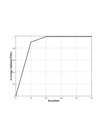
(a) Average optimal policy $\pi_{t}(a|s)$

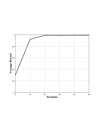
(b) Average reward $\mathcal{R}\big{(}\mathcal{S}_{t},\mathcal{A}_{t}\big{)}$

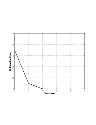
(c) Error for Q-function $\mathcal{Q}_{t}(s,a)$

Figure 3: Reward, policy and Q-function error versus the iteration regime, while $|\mathcal{S}|=\mathscr{U}_{0}+\mathscr{V}_{0}=5+7=12$, $|\mathcal{A}|=max\{\mathscr{U}_{0},\mathscr{V}_{0}\}=7$, $\mathcal{V}_{ensembel}(\zeta)=\zeta^{2}$.

Finally speaking, in Fig. 3, and the subfigures a, b and c the average reward $\mathcal{R}\big{(}\mathcal{S}_{t},\mathcal{A}_{t}\big{)}$, the error in relation to the Q-function $\mathcal{Q}_{t}(s,a)$, i.e., $\frac{\mathcal{Q}_{t}-\mathcal{Q}^{\star}}{\mathcal{Q}^{\star}}$ and the average optimal policy $\pi_{t}(a|s)$ $-$ while $(\cdot)^{\star}$ stands for the optimum-value $-$ are respectively depicted versus the iteration regime while $|\mathcal{S}|=\mathscr{U}_{0}+\mathscr{V}_{0}=5+7=12$, $|\mathcal{A}|=max\{\mathscr{U}_{0},\mathscr{V}_{0}\}=7$, $\mathcal{V}_{ensembel}(\zeta)=\zeta^{2}$ are basically selected.

V conclusion

A new bound and the relating interpretations over the concave version of the SOP maximisation problem were fundamentally explored in this paper. We technically considered a Riemannian mani-fold for the SOP’s concave version and a volume for it. Towards such end, some highly professional and insightful principles such as Keyhole contour, Finsler’s lemma, the generalised Brunn-Minkowski inequality etc were used. In order to find the optimal policy in relation to the eigenvalue distributions, a novel Markov decision process based reinforcement learning algorithm was also essentially proposed $-$ something that was subsequently extended to a possibilisitically semi-Markov decision process for the case of periodic attacks and with regard to the possibility-theory.

Appendix A Proof of Lemma 1

The proof is performed according to the Taylor expansion of

$$\begin{split}\;e^{\mathscr{t}\Lambda}{\color[rgb]{0,0,0}\;=\;}1+\mathscr{t}\Lambda{\color[rgb]{0,0,0}\;+\;\mathscr{O}\{\cdot\}},\end{split}$$ (17)

while $\mathscr{O}\{\cdot\}$ is the Big-O notation. Now, by applying an expected-value operand, we consequently reach out

$$\begin{split}\;\mathbb{E}\big{\{}\Lambda\big{\}}{\color[rgb]{0,0,0}\;\leq\;}\frac{\mathbb{E}\big{\{}e^{\mathscr{t}\Lambda}\big{\}}-1}{\mathscr{t}}.\end{split}$$ (18)

The proof is now completed.$\;\;\;\blacksquare$

Appendix B Proof of Lemma 4

The cumulative distribution function (CDF)

$$\begin{split}\;\mathscr{F}_{\Lambda}(\lambda)=\mathbb{P}\mathscr{r}\big{(}\Lambda\leq\lambda\big{)}\;\;\;\;\;\;\;\;\;\\ =1-\mathbb{P}\mathscr{r}\big{(}\Lambda\geq\lambda\big{)}\;\;\;\\ =1-e^{-\mathscr{t}\Lambda}\mu_{\Lambda}(\mathscr{t})\;\;,\end{split}$$ (19)

holds while $\mu_{\Lambda}(\mathscr{t})$ is the moment-generating function (MGF), so, we have

$$\begin{split}\;\mathbb{E}\big{\{}e^{\mathscr{t}\Lambda}\big{\}}=e^{\mathscr{t}\lambda}\mathbb{P}\mathscr{r}\big{(}\Lambda\geq\lambda\big{)},\end{split}$$ (20)

holds.

The proof is now completed.$\;\;\;\blacksquare$

Appendix C Proof of Lemma 5

Let us assume that we have the optimisation problem of $\mathop{{\rm\mathbb{M}ax}}\limits_{\Delta=\big{\{}\lambda_{1},\cdots,\lambda_{n}\big{\}}}{\rm\;}\mathbb{E}\Big{\{}\mathbb{V}\mathscr{ol}\big{\{}\Lambda\big{\}}\Big{\}}$, something that is equivalent to the maximisation over its supremum as in

$$\begin{split}\;\mathop{{\rm\mathbb{M}ax}}\limits_{\Delta=\big{\{}\lambda_{1},\cdots,\lambda_{n}\big{\}}}{\rm\;}\mathbb{V}\mathscr{ol}\Big{\{}\frac{\mathbb{E}\big{\{}e^{\mathscr{t}\Lambda}\big{\}}-1}{\mathscr{t}}\Big{\}},\end{split}$$ (21)

or with the aid of Lemma 4 $-$ the Eqn. 7 $-$ , as in

$$\begin{split}\;\mathop{{\rm\mathbb{M}ax}}\limits_{\Delta=\big{\{}\lambda_{1},\cdots,\lambda_{n}\big{\}}}{\rm\;}\mathbb{V}\mathscr{ol}\Big{\{}\frac{e^{\mathscr{t}\lambda}\mathbb{P}\mathscr{r}\big{(}\Lambda\geq\lambda\big{)}-1}{\mathscr{t}}\Big{\}},\end{split}$$ (22)

or

$$\begin{split}\;\mathop{{\rm\mathbb{M}ax}}\limits_{\Delta=\big{\{}\lambda_{1},\cdots,\lambda_{n}\big{\}}}{\rm\;}\mathbb{V}\mathscr{ol}\Big{\{}e^{\mathscr{t}\lambda}\mathbb{P}\mathscr{r}\big{(}\Lambda\geq\lambda\big{)}\Big{\}},\end{split}$$ (23)

or finally

$$\begin{split}\;\mathop{{\rm\mathbb{M}ax}}\limits_{\Delta=\big{\{}\lambda_{1},\cdots,\lambda_{n}\big{\}}}{\rm\;}\mathbb{V}\mathscr{ol}\Big{\{}e^{\mathscr{t}\lambda}\Big{\}}\mathbb{V}\mathscr{ol}\Big{\{}\mathbb{P}\mathscr{r}\big{(}\Lambda\geq\lambda\big{)}\Big{\}}.\end{split}$$ (24)

The proof is now completed.$\;\;\;\blacksquare$

Algorithm 3 A two-time-scale natural actor-critic $\epsilon-$greedy algorithm.

  Input.

• $\mathcal{S}_{0}\sim$ arbitary; $\;\;\;\;\;//$ Initial state

• $\mathcal{A}_{0}\sim\pi_{o}(\cdot|s_{0})$; $\;\;\;\;\;//$ Initial action

• $\pi_{o}(a|s)=\hat{\pi}_{o}(a|s)=\frac{1}{|\mathcal{A}|}$; $\;\;\;\;\;//$ Initial ploicy to be learnt, as the probability distribution of taking the relative action at the given state

• $T>0$; $\;\;\;\;\;//$ Iteration number

• $\alpha_{t}>0$; $\;\;\;\;\;//$ Step size

• $\beta_{t}>0$; $\;\;\;\;\;//$ Step size

• $\epsilon_{t}>0$; $\;\;\;\;\;//$ Greedy factor

• $\psi>0$; $\;\;\;\;\;//$ Discount factor

• $\mathcal{Q}_{0}(s,a)\in\mathbb{R}^{|\mathcal{S}||\mathcal{A}|}$. $\;\;\;\;\;//$ Initial Q-function corresponding to the initial policy $\pi_{o}(a|s)$

     for $t=0,1,\cdots,T$ do           Sample $\mathcal{S}_{t+1}\sim\mathcal{P}\big{(}\cdot|\mathcal{S}_{t},\mathcal{A}_{t}\big{)}$; $\;\;\;\;\;//$ According to the set of the transition probability matrices $\mathcal{P}$           Sample $\mathcal{A}_{t+1}\sim\hat{\pi}_{t}\big{(}\cdot|\mathcal{S}_{t+1}\big{)}$;           $\alpha_{t}(s,a)\leftarrow\alpha_{t}\mathbbm{1}\big{\{}\mathcal{S}_{t}=s,\mathcal{A}_{t}=a,\forall s,a\big{\}}$;           $\mathcal{Q}_{t+1}(s,a)\leftarrow\mathcal{Q}_{t}(s,a)+\alpha_{t}(s,a)\Big{[}\mathcal{R}\big{(}\mathcal{S}_{t},\mathcal{A}_{t}\big{)}+\psi\mathcal{Q}_{t}\big{(}\mathcal{S}_{t+1},\mathcal{A}_{t+1}\big{)}-\mathcal{Q}_{t}\big{(}\mathcal{S}_{t},\mathcal{A}_{t}\big{)}\Big{]},\forall s,a$; $\;\;\;\;\;//$ With regard to the Reward-function $\mathcal{R}(\cdot,\cdot)\propto f\Big{(}\frac{1}{\mathcal{P}\big{(}\zeta^{(\cdot)}_{max},\zeta^{(\cdot)}_{min}\big{)}}\Big{)}$ while $\mathcal{P}\big{(}\zeta^{(\cdot)}_{max},\zeta^{(\cdot)}_{min}\big{)}$ to be chosen           $\pi_{t+1}(a|s)\leftarrow\pi_{t}(a|s)\frac{exp\big{(}\beta_{t}\mathcal{Q}_{t+1}(s,a)\big{)}}{\sum_{a^{\prime}}\pi_{t}(a^{\prime}|s)exp\big{(}\beta_{t}\mathcal{Q}_{t+1}(s,a^{\prime})\big{)}},\forall s,a$;           $\hat{\pi}_{t+1}\leftarrow\frac{\epsilon_{t}}{|\mathcal{A}|}+(1-\epsilon_{t})\pi_{t+1}$.      endfor Sample $\hat{T}$ from $\{0,1,\cdots,T\}$ by distribution $\mathcal{P}\big{(}\hat{T}=i\big{)}=\frac{\beta_{i}}{\sum_{j=0}^{T}\beta_{j}}$. Output: $\hat{\pi}_{\hat{T}}$ end

Appendix D Proof of Proposition 1

The proof is provided here in terms of the following solution.

Where $K$ is a constant scaling factor, one can re-write the polynomial as

$$\begin{split}\;\mathscr{P}(z)=K\prod_{i=1}^{n}(z-\zeta_{i}),\end{split}$$ (25)

while $\zeta_{i},i\in\{1,\cdots,n\}$ stands literally for the $i-$th eigen-value.

Now, recall the term $\mathbb{V}\mathscr{ol}\Big{\{}\mathbb{P}\mathscr{r}\big{(}\Lambda\geq\lambda\big{)}\Big{\}}$ versus $\int\mathbb{V}\mathscr{ol}\Big{\{}\mathbb{P}\mathscr{r}\big{(}\Lambda\geq\lambda\big{)}\Big{\}}$. By differentiating $\mathscr{P}(z)$ with respect to $z$ as $\mathscr{P}^{\prime}(z)$, $\frac{\mathscr{P}^{\prime}(z)}{\mathscr{P}(z)}$ is obtained as

$$\begin{split}\;\frac{\mathscr{P}^{\prime}(z)}{\mathscr{P}(z)}=\sum_{i=1}^{n}\frac{1}{z-\zeta_{i}}.\end{split}$$ (26)

For the above equation, where $j=\sqrt{-1}$ is the imaginary unit, $\mathscr{L}\supseteq\mathbb{V}\mathscr{ol}\Big{\{}\mathbb{P}\mathscr{r}\big{(}\Lambda\geq\lambda\big{)}\Big{\}}$ is a closed anti-clockwise curve on the complex plane, and $\mathscr{C}\supseteq\int\mathbb{V}\mathscr{ol}\Big{\{}\mathbb{P}\mathscr{r}\big{(}\Lambda\geq\lambda\big{)}\Big{\}}$ is the region enclosed by $\mathscr{L}$, it is achieved as

$$\begin{split}\;\oint_{\mathscr{L}}\sum_{i=1}^{n}\frac{1}{z-\zeta_{i}}dz=\begin{cases}2\pi j,\;\;\;\;\mathsf{if}\;\zeta_{i}\in\mathscr{C},\\ 0,\;\;\;\;\;\;\;\;\mathsf{if}\;\zeta_{i}\notin\mathscr{C},\end{cases}\end{split}$$ (27)

accoring to which one can say that the number of the eigen-values in the region $\mathscr{C}$ is

$$\begin{split}\;N=\frac{1}{2\pi j}\oint_{\mathscr{L}}\frac{\mathscr{P}^{\prime}(z)}{\mathscr{P}(z)}dz\;\;\;\;\;\;\\ =\frac{1}{2\pi j}\sum_{i=1}^{n}\oint_{\mathscr{L}}\frac{1}{z-\zeta_{i}}dz.\end{split}$$ (28)

On the other hand, $\mathscr{P}^{\prime}(z)$ is obtained as [35]

$$\begin{split}\;\mathscr{P}^{\prime}(z)=det(\mathcal{B}-z\mathcal{A})Tr\Big{[}(\mathcal{B}-z\mathcal{A})^{-1}\underbrace{\frac{\partial(\mathcal{B}-z\mathcal{A})}{\partial z}}_{-\mathcal{A}}\Big{]},\end{split}$$ (29)

while $Tr[\cdot]$ stands for the trace of the matrix, something that is equivalent to

$$\begin{split}\;\mathscr{P}^{\prime}(z)=\mathscr{P}(z)Tr\Big{[}(\mathcal{B}-z\mathcal{A})^{-1}(-\mathcal{A})\Big{]},\end{split}$$ (30)

according to which one can say

$$\begin{split}\;N=\frac{1}{2\pi j}\oint_{\mathscr{L}}Tr\Big{[}(\mathcal{B}-z\mathcal{A})^{-1}(-\mathcal{A})\Big{]}dz.\end{split}$$ (31)

The last integral, i.e., the equation appeared above can be efficiently solved by some digitised methods such as the Rayleigh-Ritz method [36, 37, 38].

In order to conclude the proof, let us ultimately go over the essential relevance between the number of eigen-values and $\mathbb{V}\mathscr{ol}\Big{\{}\mathbb{P}\mathscr{r}\big{(}\Lambda\geq\lambda\big{)}\Big{\}}$ in the context of the following lemma.

Lemma 8

The number of eigen-values discussed above relies fundamentally upon $\mathbb{P}\mathscr{r}\big{(}\Lambda\big{)}$.

Proof. In relation to the term $\mathbb{V}\mathscr{ol}\Big{\{}\mathbb{P}\mathscr{r}\big{(}\Lambda\geq\lambda\big{)}\Big{\}}$, we get in hands

$$\begin{split}\;\mathbb{P}\mathscr{r}\Big{(}\big{(}\Lambda\geq\lambda\big{)}\geq\rho\Big{)}\leq 1-\frac{e^{-\rho^{2}}}{\mathbb{P}\mathscr{r}\big{(}\Lambda\big{)}}\end{split}$$ (32)

according to the Talagrand’s Concentration inequality, while $\rho$ is an arbitary threshold. This means that $\mathbb{V}\mathscr{ol}\Big{\{}\mathbb{P}\mathscr{r}\big{(}\Lambda\geq\lambda\big{)}\Big{\}}$, $\mathscr{C}$ and $\mathscr{L}$ are functions of $\Big{(}\rho;\mathbb{P}\mathscr{r}\big{(}\Lambda\big{)}\Big{)}$ $-$ something that proves Lemma 8.

Remark 4. The accuracy of evaluating the eigen-values expressed here can be fully able to be controlled by $\rho$.

The proof is now completed.$\;\;\;\blacksquare$

Appendix E Proof of Proposition 2

The sketch of the proof is given here which is similar to [40].

We know [40]

$$\begin{split}\;\mathbb{P}\mathscr{r}\big{(}L\leq(1-\tau_{2})\tau_{1}\big{)}\;\;\;\;\;\;\;\;\;\;\;\;\;\;\;\;\;\;\;\;\;\;\;\;\;\;\;\;\;\;\;\;\;\;\;\;\;\;\;\;\\ \leq exp\big{(}\frac{k}{2}(1-(1-\tau_{2})+ln(1-\tau_{2})\big{)},\end{split}$$ (33)

which can be re-casted to

$$\begin{split}\;\mathbb{P}\mathscr{r}\big{(}L\leq(1-\tau_{2})\tau_{1}\big{)}\;\;\;\;\;\;\;\;\;\;\;\;\;\;\;\;\;\;\;\;\;\;\;\;\;\;\;\;\;\;\;\;\;\;\;\;\;\;\;\;\\ \leq exp\bigg{(}\frac{k}{2}\Big{(}\tau_{2}-\big{(}\tau_{2}+\frac{\tau^{2}_{2}}{2}\big{)}\Big{)}\bigg{)},\end{split}$$ (34)

since $ln(1-x)\leq-x-\frac{x^{2}}{2},\forall\;0\leq x<1$ holds $-$ something that can conclude the proof.$\;\;\;\blacksquare$

Appendix F Proof of Proposition 3

The proof is given as the following.

We know [41]

$$\begin{split}\;tr\Big{(}(\theta^{T}-\theta^{*T})\big{(}-\Theta+Proj(\theta,\Theta)\big{)}\Big{)}<0,\end{split}$$ (35)

holds for $\theta^{*}\in[\theta^{min}_{ij}+\eta_{ij},\theta^{max}_{ij}-\eta_{ij}]$ while the trace operator $tr(\cdot)$ is a function of $-$ sum of $-$ the eigen-values related to $\theta$, that is, $\Lambda$ in our scheme and analysis.

We furthermore know that Sizes of random projections of sets, i.e., Thereom $7.7.1$ in [42] may help us to prove that if we have a bounded set $\theta\in\mathbb{R}^{r_{1}},r_{1}<r$ while $r$ was defined in Proposition 2, with a projected set $\Theta\in\mathbb{R}^{r_{2}},r_{2}<r$, with a probability of at least $1-2e^{-r_{2}}$ we have

$$\begin{split}\;diam\big{(}\Theta\theta\big{)}\leq C_{0}\Big{(}w_{s}\big{(}\theta\big{)}+\sqrt{\frac{r_{2}}{r_{1}}}diam\big{(}\theta\big{)}\Big{)},\end{split}$$ (36)

while $C_{0}$ is a constant, $diam(\cdot)$ stands for the diameter, and $w_{s}(\theta)$ denotes the Gaussian width as $\mathbb{E}\mathop{{\rm\mathbb{S}up}}\limits_{x\in\theta}{\rm\;}\langle x,\mathscr{g}\rangle,\mathscr{g}\sim\mathscr{N}(0,I_{r_{1}})$.

The proof is now completed.$\;\;\;\blacksquare$

Appendix G Proof of Proposition 4

Let us start the proof with the Gauss-Bonnet-Theorem. It says that for a manifold $\mathcal{M}$ with the boundary $\partial\mathcal{M}$, with the Euler characterisitcs $\mathcal{X}\big{(}\mathcal{M}\big{)}$ and the Gaussian Curvature $\mathcal{K}$ and the Geodesic Curvature $\mathcal{K}_{g}$ relating to $\partial\mathcal{M}$, the following is satidfied

$$\begin{split}\;\int_{\mathcal{M}}\mathcal{K}d\mathcal{S}_{area}+\int_{\partial\mathcal{M}}\mathcal{K}_{g}ds=2\pi\mathcal{X}\big{(}\mathcal{M}\big{)},\end{split}$$ (37)

while $\mathcal{S}_{area}$ stands theoretically for the area of $\mathcal{M}$ and $s\subset\mathcal{S}_{area}$.

Now, we initially see that the contractibility radius as well as the equilibrium we are supposed to go over rely deeply upon the principal curvatures, i.e., the eigen-vectors.

Additionally, Pu-1952 inquality says that the Systol of a manifold $\mathcal{M}$ as $\mathcal{SYS}\big{(}\mathcal{M}\big{)}$ as the least lenght of a non-contractible loop of the homeomorphic manifold $\mathcal{M}$ $-$ to the real projective plan $-$ , i.e., the lowerbound of the lenghts of non-contractible closed curves over $\mathcal{M}$ satisfies

$$\begin{split}\;\mathcal{S}_{area}\geq\frac{2}{\pi}\mathcal{SYS}^{2}\big{(}\mathcal{M}\big{)},\end{split}$$ (38)

while the equlity holds for the constant Gaussian curvatures, i.e., when $\mathcal{M}$ is locally isometric. Or correspondingly,

$$\begin{split}\;\mathcal{C}_{n}\Big{(}\mathbb{V}\mathscr{ol}\big{(}\mathcal{M}\big{)}\Big{)}^{\frac{1}{n}}\geq\mathcal{SYS}\big{(}\mathcal{M}\big{)},\exists\mathcal{C}_{n}\in\mathbb{R}^{n}.\end{split}$$ (39)

Thus, it has so far been proven that, in order to work on the contractibility radius as well as the equilibrium discussed above, it is necessary and sufficient for us to only focus on the eigen-vectors.

Now, in every kind of manifold and space, there may exist multiple maximum-eigenvalues or/and minimum-eigenvalues, for example, a hemisphere has $3$ maximum-eigenvalues and only $1$ minimum-eigenvalue. However, the distribution of the eigenvlaues may be totally different in every case. Thus, there may exist a Markov-Decision-Process $-$ something that technically enforces us to propose the following Reinforcement-learning based algorithm to find the perfect policy according to the eigenvalues’ distributions.

In relation to Algorithm 3, the reward function $\mathcal{R}(\cdot,\cdot)$ plays a vital role. Regarding the fact that we aim at finding an equilibrium as discussed above, and due to the fact that in equilibria, the maximum-eigenvalues and the minimum ones tend to get closer to each other as much as possible, one may select the reward function $\mathcal{R}(\cdot,\cdot)$ as $f\Big{(}\frac{1}{\mathcal{P}\big{(}\zeta^{(\cdot)}_{max},\zeta^{(\cdot)}_{min}\big{)}}\Big{)}$ while $\mathcal{P}\big{(}\zeta^{(\cdot)}_{max},\zeta^{(\cdot)}_{min}\big{)}$ stands fundamentally for the joint probability distribution for the maximum-eigenvalues and the minimum ones $-$ something that is writen as $\mathcal{P}\big{(}\zeta^{(\cdot)}_{max},\zeta^{(\cdot)}_{min}\big{)}\stackrel{{\scriptstyle def}}{{=}}\prod_{\mathscr{u}}\prod_{\mathscr{v}}|\zeta^{(\mathscr{v})}_{max}-\zeta^{(\mathscr{u})}_{min}|^{\beta}\prod_{\mathscr{u}+\mathscr{v}}e^{-\beta\frac{\mathscr{U}_{0}+\mathscr{V}_{0}}{2}}\mathcal{V}_{ensembel}(\zeta),\mathscr{u}\in\{1,\cdots,\mathscr{U}_{0}\},\mathscr{v}\in\{1,\cdots,\mathscr{V}_{0}\}$ while $\beta$ is the Dyson index and $\mathcal{V}_{ensembel}(\zeta)$ is theoretically the variant ensemble which is e.g. for Gaussian case $\zeta^{2}$.

Corollary 2 $-$ Example 1. In case of $\mathcal{X}\big{(}\mathcal{M}\big{)}=1$, the principal eigenvalues and the term $\int_{\mathcal{M}}\mathcal{K}d\mathcal{S}_{area}+\int_{\partial\mathcal{M}}\mathcal{K}_{g}ds$ expressed before have a structure such as $\oint\frac{2}{1+x^{2}}dx$ $-$ something that is well-routine for information-theoretic schemes such as the dirty-paper-coding-principle. According to what we have gone over in Definition 2, this case guarantees the convexity over the secrecy rate.

Corollary 3 $-$ Example 2. In case of $\mathcal{X}\big{(}\mathcal{M}\big{)}=0$ e.g. for Torus or Kelin-Bottle, regarding the inequality $\mathcal{S}_{area}\geq\frac{2}{\pi}\mathcal{SYS}^{2}\big{(}\mathcal{M}\big{)}$, it is proven that one should send little amount of information in the sense that a less amount of information leaked by Eve can be guaranteed, aimed at reducing the amount of non-contractibility and tits relative radius. This case and interpretation can be proven as follows according to the Excision-Theorem. This theorem says that if $\mathcal{M}_{0}\subset\mathcal{M}_{1}\subset\mathcal{M}$, we say $\mathcal{M}_{0}$ can be excised if the inclusion map $\big{(}\mathcal{M}\setminus\mathcal{M}_{0},\mathcal{M}_{1}\setminus\mathcal{M}_{0}\big{)}$ has an isomorphism relationship with $\big{(}\mathcal{M},\mathcal{M}_{1}\big{)}$. This kind of interpretation can also be proven by the concept of symplectic capacity as described in the following remark.

Remark 5 $-$ Symplectic capacity. The principle of Symplectic capacity falls in finding a contractible periodic orbit whose period bounds the Hofer-Zehnder capacity on the energy level which is related to the cylindrical capacity as follows. It says for $\mathcal{M}_{0}\subset\mathcal{M}_{1}\subset\mathcal{M}$, the following capacity inequality holds while $\mathcal{C}_{apacity}$ denotes the capacity: $\frac{\mathcal{C}_{apacity}\big{(}\mathcal{M}_{1}\big{)}}{\mathcal{C}_{apacity}\big{(}\mathcal{M}_{0}\big{)}}\leq\Big{(}\frac{\mathbb{V}\mathscr{ol}\big{(}\mathcal{M}\big{)}}{\mathbb{V}\mathscr{ol}\big{(}\mathcal{M}_{0}\big{)}}\Big{)}^{\frac{1}{n}}$.

Corollary 4 $-$ Example 3. In case of complex or/and imaginary values such as $\mathcal{X}\big{(}\mathcal{M}\big{)}=i$, the principal eigenvalues and the term $\int_{\mathcal{M}}\mathcal{K}d\mathcal{S}_{area}+\int_{\partial\mathcal{M}}\mathcal{K}_{g}ds$ expressed before have a structure such as $\oint\frac{1}{x}dx$ $-$ something that may result in creation of bifurcations in eigenvalues.

Remark 6 $-$ Conformal equivalence for curvatures. Two metrics $\mathscr{g}_{0}$ and $\mathscr{g}_{\phi}$ are conformally equivalent if $\mathscr{g}_{\phi}=e^{2\phi}\mathscr{g}_{0}$ holds while $e^{2\phi}$ is called the conformal factor. Now, the following is satisfied for the relative curvatures [60]: $\mathcal{K}_{\phi}=e^{2\phi}\big{(}\mathcal{K}_{0}-\Delta\phi\big{)}$ while $\Delta\phi$ is the Laplacian on the relative surface.

Remark 7 $-$ Davis-Kahan-Theorem. Assume $\mathcal{M}_{0}\subset\mathcal{M}$ and $\mathcal{M}_{1}\subset\mathcal{M}$ while $\mathcal{M}_{0}$ and $\mathcal{M}_{1}$ are not necessarily equal nor subsets of each other. There exists the following in relation to the eigen-vectors $\mathscr{v}$ of $\mathcal{M}_{0}$ and $\mathcal{M}_{1}$

$$\begin{split}\;sin\measuredangle\big{(}\mathscr{v}_{i}(\mathcal{M}_{0}),\mathscr{v}_{i}(\mathcal{M}_{1})\big{)}\leq\frac{2}{\gamma_{x}}||\mathcal{M}_{0}-\mathcal{M}_{1}||,\\ \gamma_{x}>0\;\stackrel{{\scriptstyle def}}{{=}}\mathop{{\rm\mathbb{M}in}}\limits_{j\neq i}{\rm\;}|\zeta_{i}(\mathcal{M}_{1})-\zeta_{j}(\mathcal{M}_{0})|,\;\;\;\;\;\;\;\;\;\;\end{split}$$ (40)

while $\gamma_{x}>0$ is defined as the least separation distance of the largest eigen-value(s) from the rest of the spectrum.

The proof is now completed.$\;\;\;\blacksquare$

Appendix H Proof of Proposition 5

If the attack is a denial-of-service one and if it is perodic, as fully discussed e.g. in [61], there consequently exist two totally i.i.d and separate scenraios in termf of two separately unstable and stable sub-systems between which there is a switching case. Now regarding the facts that:

• (i) the switching case theoretically entails a semi-Markov model; and

• (ii) the frequency of the occurrence in relation to our Markov model may be unavailable, that is, our knowledge of the information is somehow incomplete, the probability-theory is totally inappropriate here, we consequently need to extend the probability transitions to the possibilities ones $-$ where the transitions stand for the strength and casuality $-$ and from a possibility-theoretic point of view;

one can extend the Markov model discussed in the previous part as below.

Provisionally speaking, re-call $\mathcal{P}\big{(}\zeta^{(\cdot)}_{max},\zeta^{(\cdot)}_{min}\big{)}$ from Appendix G. Now, if we are supposed to extend the Markov process $\mathcal{F}\big{(}\zeta_{set}\big{)},\;(\cdot)_{set}\in\{min,max\}$ to a semi-Markov one, while the timing jumps are randomly distributed as well, that is, $\mathcal{F}\big{(}\zeta_{set}\big{)}$ is only valid as follows

$$\begin{split}\begin{cases}\mathcal{F}\big{(}\zeta_{set}(t)\big{)},\forall t_{s}\leq t<\forall t_{s+1},\\ \mathscr{p}_{ij}\stackrel{{\scriptstyle def}}{{=}}\mathbb{P}\mathscr{r}\big{(}\zeta^{(s+1)}_{set}=j,t_{s+1}-t_{s}\leq t|\zeta^{(s)}_{set}=i\big{)}=\\ \;\;\;\;\;\;\;\;\;\;\mathbb{P}\mathscr{r}\big{(}\zeta^{(s+1)}_{set}=j|\zeta^{(s)}_{set}=i\big{)},\end{cases}\end{split}$$ (41)

while $(\cdot)_{s}$ stands for the $s-$th state.

Remark 8 $-$ An overview over the possibility theory [63]-[67]. The following main rules hold in the possibility-theory: (i) the normality axiom indicates that $\upsilon(s)=1,\forall s\in\mathcal{S}$ holds; (ii) the non-negativity axiom indicates that $\upsilon(\varnothing)=0$; (iii) degree of possibility is derived by $\Upsilon(\mathcal{S})=\mathop{{\rm\mathbb{S}up}}\limits_{s\in\mathcal{S}}\upsilon(s)$; (iv) degree of possibility is derived by $\Upsilon^{(nec)}(\mathcal{S})=1-\mathop{{\rm\mathbb{I}nf}}\limits_{s\notin\mathcal{S}}\upsilon(s)$; (v) the maxitivity axiom says that $\Upsilon(\mathcal{S}_{1}\cup\mathcal{S}_{2})=max\big{\{}\Upsilon(\mathcal{S}_{1}),\Upsilon(\mathcal{S}_{2})\big{\}},\forall\mathcal{S}_{1},\mathcal{S}_{2}\subseteq\mathcal{S}$; (vi) the minitivity axiom says that $\Upsilon(\mathcal{S}_{1}\cap\mathcal{S}_{2})=min\big{\{}\Upsilon(\mathcal{S}_{1}),\Upsilon(\mathcal{S}_{2})\big{\}},\forall\mathcal{S}_{1},\mathcal{S}_{2}\subseteq\mathcal{S}$. Furthermore, the following conditional properties are information-theoretically satisfied [67]

$$\begin{split}\upsilon(s^{(i)}_{1},s^{(j)}_{2})=\upsilon(s^{(j)}_{2}|s^{(i)}_{1})\upsilon(s^{(i)}_{1}),\;\;\;\;\;\;\;\;\;\;\;\;\;\;\;\;\;\;\;\;\;\;\\ \upsilon(s^{(i)}_{1})=\frac{1}{\varpi_{1}(s^{(i)}_{1})}\mathop{{\rm\mathbb{M}ax}}\limits_{s^{(j)}_{2}}\upsilon(s^{(i)}_{1},s^{(j)}_{2}),\;\;\;\;\;\;\;\;\;\;\\ \upsilon(s^{(j)}_{2})=\frac{1}{\varpi_{2}(s^{(j)}_{2})}\mathop{{\rm\mathbb{M}ax}}\limits_{s^{(i)}_{1}}\upsilon(s^{(i)}_{1},s^{(j)}_{2}),\;\;\;\;\;\;\;\;\;\\ \varpi_{1}(s^{(i)}_{1})=\mathop{{\rm\mathbb{M}ax}}\limits_{s^{(j)}_{2}}\upsilon(s^{(j)}_{2}|s^{(i)}_{1})\leq 1,\;\;\;\;\;\;\;\;\;\;\;\;\;\;\;\;\;\;\\ \varpi_{2}(s^{(j)}_{2})=\mathop{{\rm\mathbb{M}ax}}\limits_{s^{(i)}_{1}}\upsilon(s^{(i)}_{1}|s^{(j)}_{2})\leq 1,\;\;\;\;\;\;\;\;\;\;\;\;\;\;\;\;\;\;\\ \upsilon(s^{(i)}_{1}|s^{(j)}_{2})=\frac{\upsilon(s^{(i)}_{1})\upsilon(s^{(j)}_{2}|s^{(i)}_{1})}{\upsilon(s^{(j)}_{2})}\;\;\;\;\;\;\;\;\;\;\;\;\;\;\;\;\;\;\;\;\;\\ =\frac{\varpi_{2}(s^{(j)}_{2})\upsilon(s^{(i)}_{1})\upsilon(s^{(j)}_{2}|s^{(i)}_{1})}{\mathop{{\rm\mathbb{M}ax}}\limits_{s^{(k)}_{1}}\big{\{}\upsilon(s^{(k)}_{1})\upsilon(s^{(j)}_{2}|s^{(k)}_{1})\big{\}}},\;\;\;\;\;\;\;\\ \end{split}$$ (42)

as well as [67]

$$\begin{split}\upsilon(s^{(k)}_{3}|s^{(i)}_{1})=\frac{1}{\varpi_{3}(s^{(i)}_{1})}\mathop{{\rm\mathbb{M}ax}}\limits_{s^{(j)}_{2}}\upsilon(s^{(k)}_{3}|s^{(j)}_{2})\upsilon(s^{(j)}_{2}|s^{(i)}_{1}),\\ \varpi_{3}(s^{(i)}_{1})=\mathop{{\rm\mathbb{M}ax}}\limits_{s^{(j)}_{2}}\upsilon(s^{(j)}_{2}|s^{(i)}_{1})\leq 1,\;\;\;\;\;\;\;\;\;\;\;\;\;\;\;\;\;\;\;\;\;\;\;\;\;\end{split}$$ (43)

and [67]

$$\begin{split}\mathop{{\rm\mathbb{M}ax}}\limits_{s^{(j)}_{2}}\upsilon(s^{(k)}_{3},s^{(j)}_{2}|s^{(i)}_{1})=\;\;\;\;\;\;\;\;\;\;\;\;\;\;\;\;\\ \mathop{{\rm\mathbb{M}ax}}\limits_{s^{(j)}_{2}}\upsilon(s^{(k)}_{3}|s^{(j)}_{2},s^{(i)}_{1})\upsilon(s^{(j)}_{2}|s^{(i)}_{1})=\\ \mathop{{\rm\mathbb{M}ax}}\limits_{s^{(j)}_{2}}\upsilon(s^{(k)}_{3}|s^{(j)}_{2})\upsilon(s^{(j)}_{2}|s^{(i)}_{1}),\end{split}$$ (44)

which is also equal to [67]

$$\begin{split}\mathop{{\rm\mathbb{M}ax}}\limits_{s^{(j)}_{2}}\upsilon(s^{(j)}_{2}|s^{(k)}_{3},s^{(i)}_{1})\upsilon(s^{(k)}_{3}|s^{(i)}_{1})=\\ \mathop{{\rm\mathbb{M}ax}}\limits_{s^{(j)}_{2}}\upsilon(s^{(j)}_{2}|s^{(i)}_{1})\upsilon(s^{(k)}_{3}|s^{(i)}_{1})=\\ \varpi_{3}(s^{(i)}_{1})\upsilon(s^{(k)}_{3}|s^{(i)}_{1}).\;\;\;\;\;\;\;\;\;\;\;\;\;\end{split}$$ (45)

In addition, the following equations are also added [68, 69]

$$\begin{split}\upsilon(s_{1}|s_{2}\cdots,s_{N})=\begin{cases}\frac{\upsilon(s_{1},\cdots,s_{N})}{\upsilon(s_{2},\cdots,s_{N})},\;\upsilon(s_{2},\cdots,s_{N})\neq 0,\\ 1,\;\;\;\;\;\;\;\;\;\;\;\;\;\;\;\upsilon(s_{2},\cdots,s_{N})=0,\end{cases}\end{split}$$ (46)

as well as

$$\begin{split}\upsilon(s_{1},\cdots,s_{N})=\prod_{i}\upsilon\big{(}s_{i}|\mathscr{Par}(s_{i})\big{)},\end{split}$$ (47)

while the parent elements $\mathscr{Par}(s_{i})$ are the ones defined by the Cartesian poruct of the main set’s domain, aacording to the following definition for the possibilistic graphs.

Definition 5: Possibilistic graph [68, 69]. A possibilistic casual network is defined in terms of the graph $\mathscr{G}_{\mathscr{poss}}\stackrel{{\scriptstyle def}}{{=}}\bigg{\{}\Big{(}s,\mathscr{Par}(s),\alpha_{\mathscr{poss}}\Big{)}:\upsilon\big{(}s|\mathscr{Par}(s)\big{)}=\alpha_{\mathscr{poss}}\neq 1\bigg{\}}$.

The proof is now completed.$\;\;\;\blacksquare$

References

• [1] Y. Ai, A. Mathur, L. Kong, ”Secure Outage Analysis of FSO Communications Over Arbitrarily Correlated Málaga Turbulence Channels,” IEEE Trans. Vehicular Technol., Vol. 70, no. 4, pp. 3961-3965, 2021.
• [2] Y. Ai, F. A. P. deFigueiredo, L. Kong, ”Secure Vehicular Communications Through Reconfigurable Intelligent Surfaces,” IEEE Trans. Vehicular Technol., Vol. 70, no. 4, pp. 7272-7276, 2021.
• [3] L. Yang, J. Yang, W. Xie, ”Secrecy Performance Analysis of RIS-Aided Wireless Communication Systems,” IEEE Trans. Vehicular Technol., Vol. 69, no. 10, pp. 12296-12300, 2020.
• [4] I. Trigui, W. Ajib, W. Zhu, ”Secrecy Outage Probability and Average Rate of RIS-Aided Communications Using Quantized Phases,” IEEE Commun. Letters, Vol. 25, no. 6, pp. 1820-1824, 2021.
• [5] S. Kavaiya, D. K. Patel, Z. Ding, Y. L. Guan, ”Physical Layer Security in Cognitive Vehicular Networks,” IEEE Trans. Commun., Vol. 69, no. 4, pp. 2557-2569, 2021.
• [6] K. Lee, J. Bang, H. Choi, ”Secrecy Outage Minimization for Wireless-Powered Relay Networks With Destination-Assisted Cooperative Jamming,” IEEE IoT. J., Vol. 8, no. 3, pp. 1467-1476, 2021.
• [7] R. K. Ahiadormey, P. Anokye, H. Jo, C. Song, ”Secrecy Outage Analysis in NOMA Power Line Communications,” IEEE Commun. Letters, Vol. 25, no. 5, pp. 1448-1452, 2021.
• [8] R. Ruby, Q. Pham, K. Wu, A. A. Heidari, H. Chen, ”Enhancing Secrecy Performance of Cooperative NOMA-based IoT Networks via Multi-Antenna Aided Artificial Noise,” IEEE IoT. J., Vol. pp, no. 99, pp. 1-1, 2022.
• [9] K. Guo, K. An, F. Zhou, T. A. Tsiftsis, G. Zheng, ”On the Secrecy Performance of NOMA-Based Integrated Satellite Multiple-Terrestrial Relay Networks With Hardware Impairments,” IEEE Trans. Vehicular Technol., Vol. 70, no. 4, pp. 3661-3676, 2021.
• [10] X. Lai, L. Fan, X. Lei, Y. Deng, G. K. Karagiannidis, ”Secure Mobile Edge Computing Networks in the Presence of Multiple Eavesdroppers,” IEEE Trans. Commun., Vol. pp, no. 99, pp. 1-1, 2022.
• [11] G. Sharma, N. Pandey, A. Singh, R. K. Mallik, ”Secrecy Optimization for Diffusion-Based Molecular Timing Channels, ” IEEE Trans. Molecular, Bio. Multi. Commun., Vol. 7, no. 4, pp. 253-261, 2021.
• [12] Y. Lou, R. Sun, J. Cheng, D. Nie, G. Qiao, ”Secrecy Outage Analysis of Two-Hop Decode-and-Forward Mixed RF/UWOC Systems,” IEEE Commun. Letters, Vol. pp, no. 9, pp. 1-1, 2022.
• [13] T. Lu, L. Chen, J. Zhang, K. Cao, ”Reconfigurable Intelligent Surface Assisted Secret Key Generation in Quasi-Static Environments,” IEEE Commun. Letters, Vol. 26, no. 2, pp. 244-248, 2022.
• [14] M. Zamanipour, "A Novelty in Blahut-Arimoto Type Algorithms: Optimal Control over Noisy Communication Channels," IEEE Trans. Vehicular Technol. Vol. 69, no. 6, pp. 6348-6358, 2020.
• [15] P. Algoet, T. Cover, ”A Sandwich Proof of the Shannon-McMillan-Breiman Theorem,” The Annals of Probability. Vol. 16, no. 2, pp. 899-909, 1988.
• [16] S. Verdu, T. Han, ”The Role of the Asymptotic Equipartition Property in Noiseless Source Coding,” IEEE Trans. Info. Theory, Vol. 43, no. 3, pp. 847-857, 1997.
• [17] J. Wang, Z. Xie, G. Yu, ”Decay of scalar curvature on uniformly contractible manifolds with finite asymptotic dimension,” https://arxiv.org/abs/2101.11584, 2021.
• [18] B. Tosun, ”Stein domains in $\mathbb{C}^{2}$ with prescribed boundary,” Adv. Geom., Vol. 22, no. 1, pp. 9-22, 2022.
• [19] J. M. Lee, ”Introduction to smooth manifolds,” G. Texts. Math., 2012.
• [20] G. Naber, ”Topological methods in Euclidean spaces,” Dover, 2000.
• [21] A. Tsiamis, K. Gatsis, G. J. Pappas, ”State-Secrecy Codes for Networked Linear Systems,” IEEE Trans. Auto. Control, Vol. 65, no. 5, pp. 2001-2015, 2020.
• [22] B. Anderson, J. Moore, ”Optimal filtering,” Prentice-Hall, 1979.
• [23] H. Sun, Z. Wang, ”Minimal Euler Characteristics of 4-manifolds with 3-manifold groups,” https://arxiv.org/abs/2103.10273, 2021.
• [24] R. Caniato, T. Riviere, ”The Unique Tangent Cone Property for Weakly Holomorphic Maps into Projective Algebraic Varieties,” https://arxiv.org/abs/2108.10371, 2021.
• [25] G. Olikier, P. Absil, ”On the continuity of the tangent cone to the determinantal variety,” https://arxiv.org/abs/2201.03979, 2022.
• [26] F. Fillastre, ”Gauss images of hyperbolic cusps with convex polyhedral boundary,” Trans. American Math., Vol. 363, no. 10, pp. 5481-5536, 2011.
• [27] B. Anderson, M. Ye, ”Exterma without convexity and stability without Lyapunov,” Com. Info. Sys., Vol. 20, no. 3, 2020.
• [28] C. Byrnes, ”On brockett’s necessary condition for stabilizability and the topology of Lyapunov functions on $\mathbb{R}^{n}$,” Com. Info. Sys., Vol. 8, no. 4, pp. 333-352, 2008.
• [29] R. A. Vitale, ”The Brunn-Minkowski inequality for random sets,” J. Multivariate Anal., Vol. 33, no. 2, pp. 286-293, 1990.
• [30] S. Boyd, S. P. Boyd, and L. Vandenberghe, ”Convex Optimization.” Cambridge University Press, 2004
• [31] W. Liu, ”Decay rates of energy of the 1D damped original nonlinear wave equation,” Nonlinear Anal. Real W. Apps., Vol. 63, pp. 103-412, 2022.
• [32] H. J. van Waarde, M. K. Camlibel, ”A Matrix Finsler’s Lemma with Applications to Data-Driven Control,” https://arxiv.org/abs/2103.13461, 2021.
• [33] T. S. Blyth, E. F. Robertson, Basic Linear Algebra, 2nd ed., Springer, 1998.
• [34] L. V. Ahlfors, Complex Analysis, 2nd ed., New York: McGraw-Hill, 1970.
• [35] K. Petersen, M. Pedersen, The Matrix Cookbook, http://matrixcookbook.com, 2012.
• [36] Y. Li, G. Geng, Q. Jiang, ”A Parallelized Contour Integral Rayleigh–Ritz Method for Computing Critical Eigenvalues of Large-Scale Power Systems,” IEEE Trans. Smart Grid, Vol. 9, no. 4, pp. 3573-3581, 2018.
• [37] T. Ikegami, T. Sakurai, “Contour Integral Eigensolver for Non-Hermitian Systems: a Rayleigh-Ritz-type Approach,” Taiwanese J. Math., vol. 14, no. 3A, pp. 825-837, 2010.
• [38] Y. Li, G. Geng, Q. Jiang, ”A Parallel Contour Integral Method for Eigenvalue Analysis of Power Systems,” IEEE Trans. Power Sys., Vol. 32, no. 1, pp. 624 - 632, 2017.
• [39] Alon, Noga, Spencer, Joel H. The Probabilistic Method 2nd ed. John Wiley & Sons, Inc., 2000.
• [40] S. Dasgupta, A. Gupta, ”An elementary proof of a theorem of Johnson and Lindenstrauss,” Random Structs. & Algs. 2002.
• [41] S. S. Tohidi, Y. Yildiz, ”Handling actuator magnitude and rate saturation in uncertain over-actuated systems: A modified projection algorithm approach,” https://arxiv.org/abs/2009.03024, 2020.
• [42] R. Vershynin, ”High-dimensional probability: An introduction with applications in data science,” Cambridge University Press, Vol. 47, 2018.
• [43] I Satake, ”The Gauss-Bonnet theorem for V-manifolds,” J. Math. S. Japan, 1957
• [44] C. Allendoerfer, A Weil, ”The gauss-bonnet theorem for riemannian polyhedra,” Trans. American Math., 1943.
• [45] M Gromov, ”Systoles and intersystolic inequalities,” Actes de la table ronde de geometrie differentielle, 1996.
• [46] K. Katz, M. Katz, ”Relative systoles of relative-essential $2-$complexes,” Alg. Geom. Topology, Vol. 11, pp. 101-999, 2011.
• [47] M. Bailey, ”Symplectic capacity and convexity”, Toronto Press, 2019.
• [48] U. Frauenfelder, ”Finitness of $\pi_{1}-$sensitive Hofer-Zehnder capacity and equivariant loop space homology,” J. F. P. Theory Apps., Vol. 19. pp. 3-15, 2017.
• [49] H. Inoue, T. Kamada, ”structural instability of friction-induced vibration by characteristics polynomial plane applied to break squeal,” J. A. Mech. Design. Sys. Man., Vol. 14, no. 1, 2020.
• [50] C Clark, ”The asymptotic distribution of eigenvalues and eigenfunctions for elliptic boundary value problems,” Siam Review, Vol. 9, no. 4, 1967.
• [51] A. Grabsch, ”General truncated linear statistics for the top eigenvalues of random matrices,” https://arxiv.org/abs/2111.09004, 2021.
• [52] E. Gundogdu, V. Constantin, S. Parashar, A. Seifoddini, M. Dang, M. Salzmann, P. Fua, ”GarNet++: Improving Fast and Accurate Static3D Cloth Draping by Curvature Loss,” IEEE Trans. Pattern Analysis Machine Intel. Vol. 44, no. 1, pp. 181-195, 2022.
• [53] S. Khodadadian, T. T. Doan, J. Romberg, S. T. Maguluri, ”Finite Sample Analysis of Two-Time-Scale Natural Actor-Critic Algorithm,” https://arxiv.org/abs/2101.10506, 2022.
• [54] M. Mehta, ”Random matrices,” Elsevier, New york, 2004.
• [55] J. Akemann, ”The Oxford handbook of random matrix theory,” Oxford University Press, 2011.
• [56] A. D. Wallace, ”The map excision theorem,” Duke Math. J. Vol. 19, no. 1, pp. 177-182, 1952.
• [57] D. Labardini-Fragoso, D. Velasco, ”On a family of Caldero-Chapoton algebras that have the Laurent phenomenon,” J. Algebra, Vol. 520, pp. 90-135,2019.
• [58] A. Blass, ”Seven trees in one,” J. P. A. Algebra, Vol. 103, pp. 1-21, 1995.
• [59] G. Cerulli Irelli, D. Labardini-Fragoso, J, Schroer, ”Caldero-Chapoton algebras,” Trans. Amer. Math. Soc. Vol. 367, pp. 2787-2822, 2015.
• [60] V. E. Coll, L. B. Whitt, ”The Flat Plane and a Constructive Proof of Minding’s Theorem,” https://arxiv.org/abs/1902.06089, 2019.
• [61] Y. Zhu, W. Zheng, ”Observer-Based Control for Cyber-Physical Systems With Periodic DoS Attacks via a Cyclic Switching Strategy,” IEEE Trans. Auto. Control, Vol. 65, no. 8, pp. 3714-3721, 2020.
• [62] S. Wang, J. Park, ”Modeling and analysis of multi-type failures in wireless body area networks with semi-Markov model,” IEEE Commun. Letters, Vol. 14, no. 1, pp. 6-8, 2010.
• [63] D. Dubois, H. Prade, ”Possibility Theory and Its Applications: Where Do We Stand?,” Springer Handbook. Comput. Intel., pp. 31-60, 2015.
• [64] L.A. Zadeh, ”Fuzzy sets as a basis for a theory of possibility,” Fuzzy Set. Syst. no. 1, pp. 3-28, 1978.
• [65] L.A. Zadeh, ”Fuzzy sets and information granularity,” Adv. Fuzzy Set Theory. Apps., pp. 3-18, 1979.
• [66] L.A. Zadeh, ”Possibility theory and soft data analysis,” Math. Fron. Social Policy Sc., pp. 69-129, 1982.
• [67] W. Mei, ”Formalization of Fuzzy Control in Possibility Theory via Rule Extraction,” IEEE Access, Vol. 7, pp. 90115-90124, 2019.
• [68] S. Benferhat, D. Dubois, L. Garcia, H. Prade, ”Possibilistic logic bases and possibilistic graphs,” https://arxiv.org/abs/1301.6679, 2013.
• [69] S. Benferhat, D. Dubois, S. Kaci, H. Prade, ”Graphical readings of possibilistic logic bases,” https://arxiv.org/abs/1301.2255, 2013.