FAST AND ACCURATE NUMERICAL SIMULATIONS FOR THE STUDY OF CORONARY ARTERY BYPASS GRAFTS BY ARTIFICIAL NEURAL NETWORK

ABBREVIATIONS

ANN	Artificial neural network
CABG	Coronary artery bypass graft
DEIM	Discrete empirical interpolation method
FE	Finite element
FFD	Free form deformation
FOM	Full order model
FV	Finite volume
LAD	Left anterior descending artery
LCx	Left circumflex artery
LITA	Left internal thoracic artery
LMCA	Left main coronary artery
NURBS	Non-uniform rational basis spline
POD	Proper orthogonal decomposition
RBF	Radial basis functions
ROM	Reduced order model
SV	Saphenous vein
WSS	Wall shear stress

1 INTRODUCTION

Coronary artery diseases represent one of the most common causes of mortality worldwide. When coronary arteries are completely or partially occluded for the presence of stenosis, the lack of blood to the cardiac tissue can lead to heart attack. Nowadays, the most successful surgical procedure consists of creating an alternative path to bypass the stenosis, the so-called CABG. In literature, different CABG configurations in presence of single or multiple stenosis are analysed in order to establish a good clinical treatment: see, e.g., d’Allonnes et al. (2002); Harling et al. (2012); Rosenblum et al. (2019); Scott et al. (2000); Gaudino et al. (2014). Since after some years from the surgical treatment blood supply fails again by causing the need of reintervention, computational investigation of haemodynamic patterns near stenosis and anastomosis regions is of remarkable clinical interest.

Our study focuses on the numerical simulation of the blood flow features in a patient-specific coronary system when an isolated stenosis of LMCA occurs. A CABG performed with the LITA on the LAD is analyzed. High fidelity simulations are able to provide accurate predictions of the blood flow. However in the clinical context repeated model evaluations at varying of physical and geometrical parameters are often required and this leads to very high computational cost when using standard discretization techniques, here referred to as FOMs, e.g. FE or FV techniques. ROMs have been proposed as an efficient tool to approximate FOM systems by significantly reducing the computational cost required to obtain numerical solutions in a parametric setting (see, e.g., Benner et al., 2015, Hesthaven et al., 2016). A non-intrusive data-driven ROM is used in this work in order to enable fast and reliable computations, involving POD for the computation of reduced basis space and ANNs for the evaluation of the modal coefficients (Chen et al., 2021; Hesthaven and Ubbiali, 2018; Shah et al., 2021; Pichi et al., 2021). Both primal variables (pressure and velocity) and derived quantities (wall shear stress) are considered. The introduction of machine learning techniques is appealing due to its development and diffusion in several areas including hemodynamic applications: see, e.g., Liang et al., 2020; Gharleghi et al., 2020; Su et al., 2020; Kissas et al., 2020. The FV method is employed due to its reliable application in some recent works (Girfoglio et al., 2020, 2021; Pandey et al., 2020; Marsden and Esmaily-Moghadam, 2015; Buoso et al., 2019) and its widespreading in commercial codes.

The chapter is organized as follows. The FOM is introduced and discussed in Section 2. Some relevant ROM studies related to similar problems to ours as well as the ROM approach here adopted are discussed in Section 3. The numerical results are shown in Section 4. Finally, conclusions and perspectives are provided in Section 5.

2 THE FULL ORDER MODEL

2.1 The Navier-Stokes equations

Let us refer to a patient-specific domain $\Omega\subset\mathbb{R}^{3}$ over a cardiac cycle $(0,T]$ when the transient effects are passed. In this work, the blood is considered as a Newtonian fluid. Then if $\mathbf{u}:\Omega\times(0,T]\mapsto\mathbb{R}^{3}$ and $P:\Omega\times(0,T]\mapsto\mathbb{R}$ are the velocity and the kinematic pressure of the fluid (i.e. the pressure divided by the density), and $\nu\in\mathbb{R}^{+}$ is the kinematic viscosity, the dynamics of the blood is described by the incompressible Navier-Stokes equations:

$$\begin{cases}\frac{\partial\bm{u}}{\partial t}+\nabla\cdot(\bm{u}\otimes\bm{u})-\nu\Delta\bm{u}+\nabla P=0&\quad\text{in}\quad\Omega\times(0,T],\\ \nabla\cdot\bm{u}=0&\quad\text{in}\quad\Omega\times(0,T].\end{cases}$$ (1)

We also introduce the WSS defined as follows:

$$\text{WSS}=\tau\cdot\mathbf{n},$$ (2)

where $\tau=\nu(\nabla\mathbf{u}+\nabla\mathbf{u}^{T})$ is the stress tensor and $\mathbf{n}$ is the unit normal outward vector.

Concerning boundary conditions, a realistic flow rate waveform was enforced on LITA and LMCA sections (see Figure LABEL:CB:a):

$$q_{i}(t)=f^{i}\bar{q}_{i}(t),\quad i=LMCA,LITA,$$ (3)

where the factor $f^{i}\in\left[\frac{2}{3},\frac{4}{3}\right]$ is adapted from Keegan et al. (2004); Ishida et al. (2001); Verim et al. (2015).

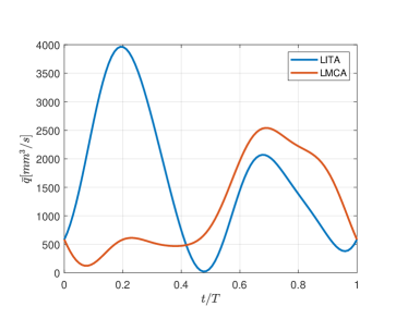
(a)

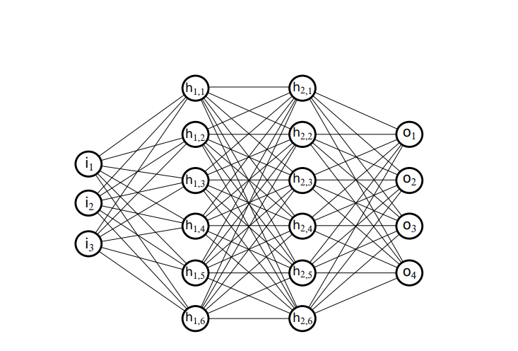
(b)

Figure 1: Time evolution over the cardiac cycle of $\bar{q}_{LMCA}$ and $\bar{q}_{LITA}$ (Keegan et al., 2004; Ishida et al., 2001) LABEL:sub@CB:a and topology of the feedforward neural network LABEL:sub@CB:b.

For the vessel wall, no slip condition is imposed and, for the outflow boundaries, LAD and LCx, homogeneous Neumann boundary conditions are prescribed (Ballarin et al., 2016, 2017).

2.2 Time and space discretization

Let us consider a time step $\Delta t\in\mathbb{R}^{+}$ such that $t^{n}=n\Delta t$, $n=0,\ldots,N_{T}$ and $T=N_{T}\Delta t$. Moreover, let $(\bm{u}^{n},P^{n})$ be the approximations of velocity and pressure at time $t^{n}$.

For the time discretization of Eqs. (1), we adopt a Backward Differentiation Formula of order 2:

$$\begin{split}\begin{cases}\frac{3}{2\Delta t}\bm{u}^{n+1}+\nabla\cdot(\bm{u}^{n}\otimes\bm{u}^{n+1})-\nu\Delta\bm{u}^{n+1}+\nabla P^{n+1}=\bm{b}^{n+1},&\\ \nabla\cdot\bm{u}^{n+1}=0.&\end{cases}\end{split}$$ (4)

where $\bm{b}^{n+1}=\frac{4\bm{u}^{n}-\bm{u}^{n-1}}{2\Delta t}$.

For the space discretization of problem (4) we adopt a FV method. The Gauss-divergence theorem allows to write the integral form of the momentum equation in each control volume $\Omega_{i}$ as follows:

$$\begin{split}\frac{3}{2\Delta t}\int_{\Omega_{i}}\bm{u}^{n+1}d\Omega+&\int_{\partial\Omega_{i}}(\bm{u}^{n}\otimes\bm{u}^{n+1})\cdot d\bm{A}-\nu\int_{\partial\Omega_{i}}\nabla\bm{u}^{n+1}\cdot d\bm{A}\\ &+\int_{\partial\Omega_{i}}P^{n+1}d\bm{A}=\int_{\Omega_{i}}\bm{b}^{n+1}d\Omega.\end{split}$$ (5)

The convective and diffusive terms are treated using a second order central scheme. If $\bm{u}_{i}^{n+1}$ and $\bm{b}_{i}^{n+1}$ indicate the average velocity and the source term in the control volume $\Omega_{i}$, $\bm{u}_{i,j}^{n+1}$ and $P_{i,j}^{n+1}$ the velocity and pressure associated to the centroid of face $j$ normalized by the volume of $\Omega_{i}$, the discretized form of the Eq. (5) can be written as:

$$\frac{3}{2\Delta t}\bm{u}_{i}^{n+1}+\sum_{j}\phi_{j}\bm{u}_{i,j}^{n+1}-\nu\sum_{j}(\nabla\bm{u}_{i}^{n+1})_{j}\cdot\bm{A}_{j}+\sum_{j}P_{i,j}^{n+1}\bm{A}_{j}=\bm{b}_{i}^{n+1},$$ (6)

where $\bm{A}_{j}$ is the surface vector of each face $j$ of the control volume and $\phi_{j}=\bm{u}_{j}^{n}\cdot\bm{A}_{j}$ is the convective flux associated to $\bm{u}^{n}$ through face $j$ of the control volume. Applying the divergence operator to Eq. (6) in semi-discretized form, i.e. with the pressure term in continuous form while all the other terms in discrete form, and introducing the continuity equation, the following Poisson equation for the pressure is derived:

$$\Delta P^{n+1}=\nabla\cdot\Big{(}-\sum_{j}\phi_{j}\bm{u}_{j}^{n+1}+\nu\sum_{j}(\nabla\bm{u}^{n+1})_{j}\cdot\bm{A}_{j}+\bm{b}^{n+1}\Big{)}.$$ (7)

Integrating Eq. (7) and applying the Gauss-divergence theorem, we obtain:

$$\sum_{j}(\nabla P^{n+1})_{j}\cdot\bm{A}_{j}=\sum_{j}\Big{(}-\sum_{j}\phi_{j}\bm{u}_{j}^{n+1}+\nu\sum_{j}(\nabla\bm{u}^{n+1})_{j}\cdot\bm{A}_{j}+\bm{b}^{n+1}\Big{)}_{j}\cdot\bm{A_{j}}.$$ (8)

We use the Pressure-Implicit with Splitting of Operators algorithm (Issa, 1986) available in OpenFOAM^® to deal with the coupled set of Eqs. (6) and (8).

2.3 The computational domain

Computed tomography images of a patient specific configuration were provided by Ospedale Luigi Sacco in Milan. The process to construct the virtual geometry (see Fig. LABEL:CABG1:a) was described in detail in Ballarin et al. (2016, 2017).

(a)

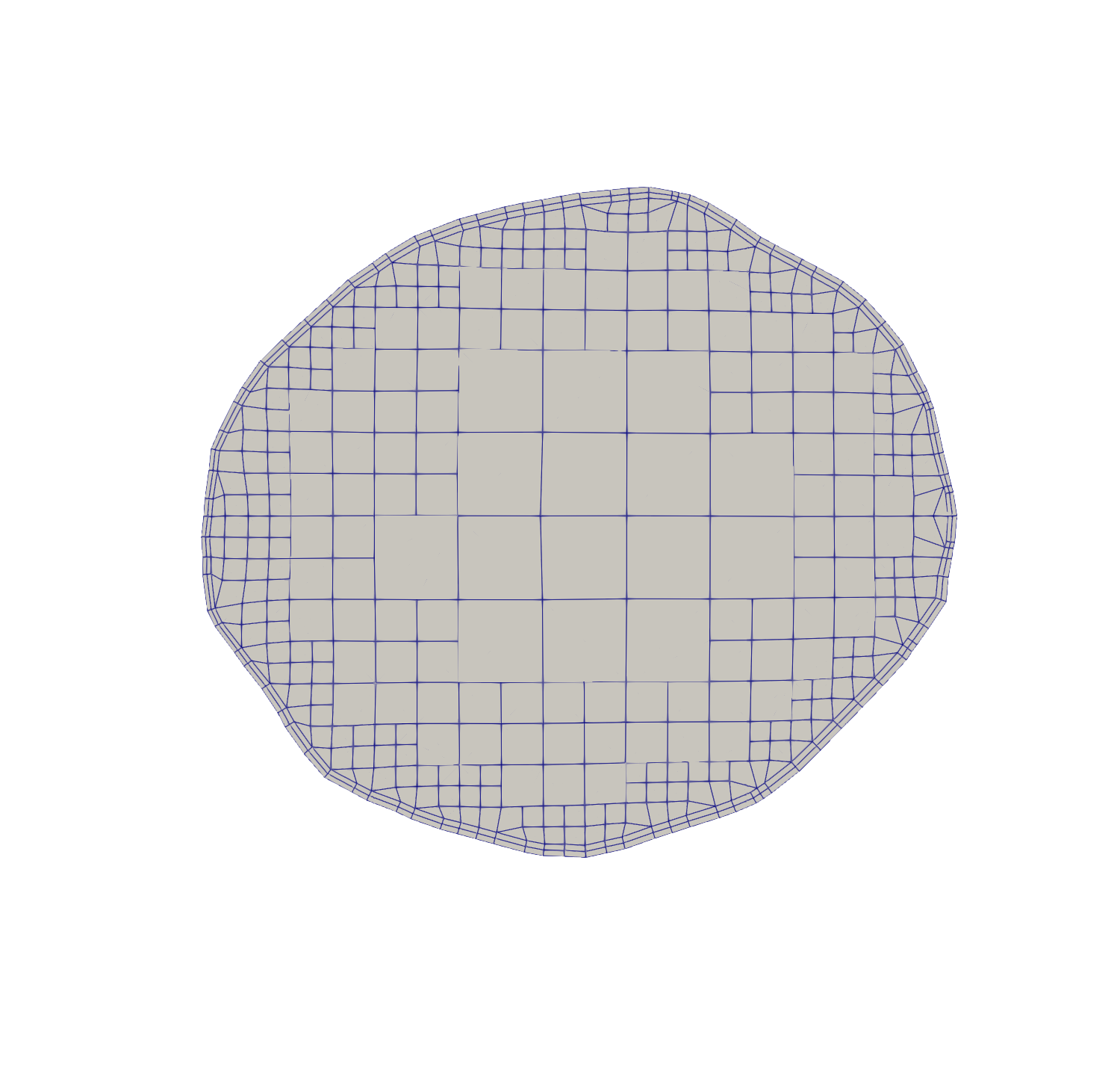
(b)

Figure 2: CABG geometry LABEL:sub@CABG1:a and view of the mesh on an internal section LABEL:sub@CABG1:b.

The mesh (Fig. LABEL:CABG1:b) is built using the mesh generation utility snappyHexMesh available in OpenFOAM^®. It has 986.278 cells and its minimum and maximum diameter are $h_{min}\simeq 3.0\cdot 10^{-5}m$ and $h_{max}\simeq 4.3\cdot 10^{-4}m$, respectively. The quality of the mesh is rather high: it has very low values of average non-orthogonality (13^∘), skewness ($\leq 3$), and aspect ratio ($\leq 16$).

In order to introduce the stenosis in the LMCA, FFD is performed by means of a NURBS volumetric parameterization (Brujic et al., 2002; Tezzele et al., 2021). The shape parametrization of the computational domain is deeply analysed in literature (Manzoni et al., 2012b; Lassila et al., 2011; Manzoni et al., 2012a; Lassila et al., 2013b, a; Manzoni et al., 2012c; Stabile et al., 2020; Burgos et al., 2015; Tezzele et al., 2018) using both FFD and RBF techniques. However, whilst the RBF approach deforms the grid as a whole and it does not preserve the original geometry, in the FFD method all the vertices remain on the initial surface.

The FFD method consists of three steps (Amoiralis and Nikolos, 2008; Lamousin and Waggenspack, 1994):

• A parametric lattice of control points is constructed generating a structured mesh around the region of the LMCA where the stenosis occurs. Then the control points are used to define a NURBS volume which contains the domain to be warped. Figure LABEL:mimmo:a displays the lattice in its initial configuration.

• The octree algorithm (Amoiralis and Nikolos, 2008) could be used to find a match between the control points of the lattice and the points of the computational domain.

• The coordinates of the control points are modified, so that the parametric volume and consequently the computational domain are deformed. Figure LABEL:mimmo:b shows the lattice in its deformed configuration where a $70\%$ stenosis is introduced.

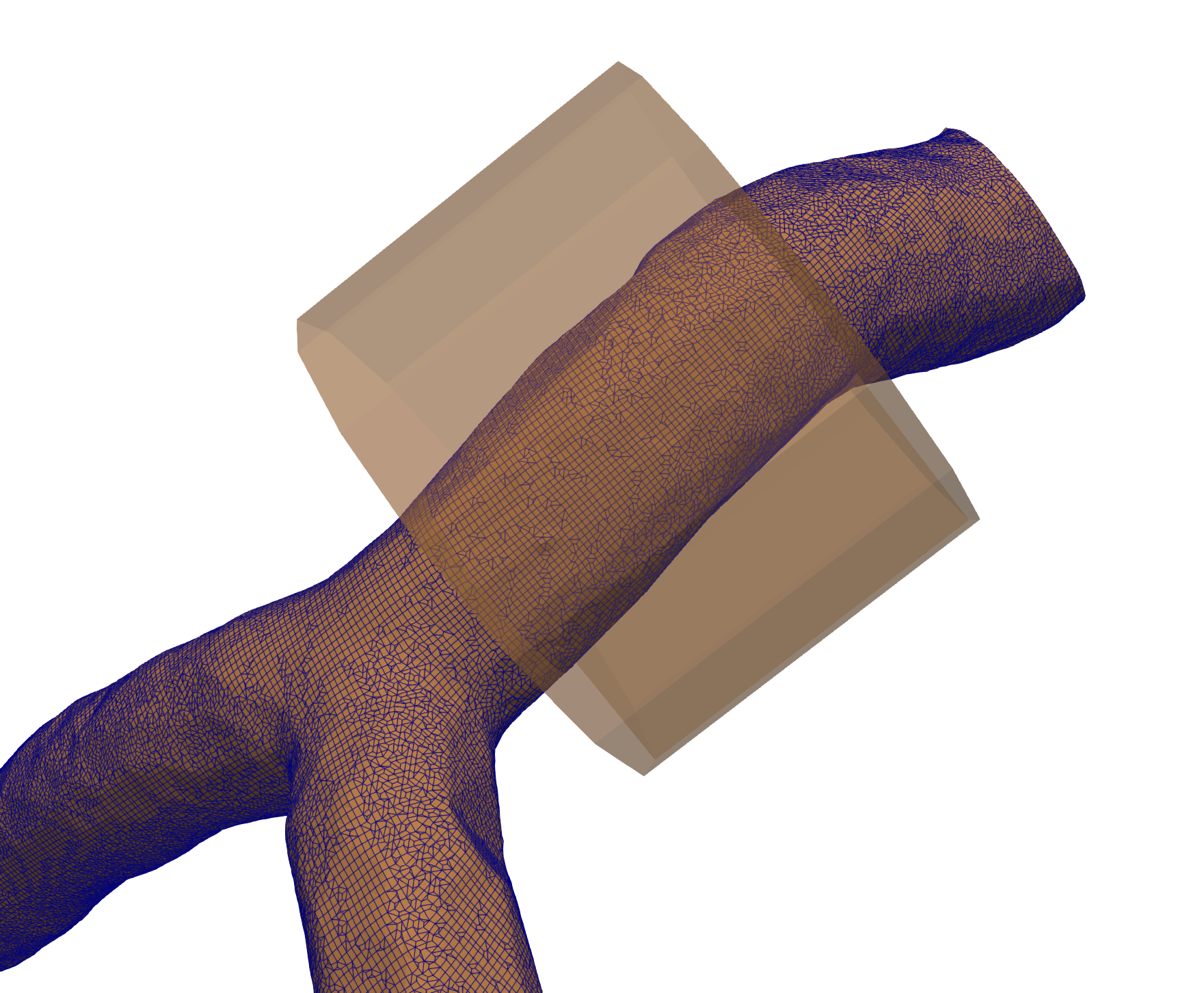
(a)

(b)

Figure 3: Introduction of $70\%$ stenosis in the LMCA using FFD technique: LABEL:sub@mimmo:a initial lattice, LABEL:sub@mimmo:b deformed lattice.

We highlight that the introduction of a $70\%$ stenosis in the LMCA does not affect the mesh quality.

3 REDUCED ORDER MODEL

3.1 POD-ANN approach

In this work we use the POD-ANN approach consisting of two main stages:

• Offline: a reduced basis space is built by applying POD to a database of high-fidelity solutions obtained by solving the FOM for different values of physical and/or geometrical parameters. Once the reduced basis space is computed, we project the original snapshots onto such a space by obtaining the corresponding parameter dependent modal coefficients. Then the training of the neural networks to approximate the map between parameters and modal coefficients is carried out. This stage is computationally expensive, however it only needs to be performed once.

• Online: for any new parameter value, we approximate the new coefficients by using the trained neural network and the reduced solution is obtained as a linear combination of the POD basis functions multiplied by modal coefficients. During this stage, it is possible to explore the parameter space at a significantly reduced cost.

Here we are going to test our ROM for the reconstruction of the time evolution of the system. So our parameter of interest coincides with the time. Other parametric studies, involving geometrical features such as the stenosis degree or physical properties such as the scaling factor $f^{i}$ (see Eq. (3)), will be addressed in a work in preparation (Siena et al., 2022).

3.1.1 Proper orthogonal decomposition and method of snapshots

We solve the FOM described in Section 2.2 for each time $t_{k}\in\{t_{1},\dots,t_{N}\}\subset(0,T]$. The high fidelity solution $\Phi_{h}=\{\mathbf{u},P,\text{WSS}\}$ can be stored into the matrix $\mathcal{S}_{\Phi}$ in a column-wise sense:

$$\mathcal{S}_{\Phi}=\{\Phi_{h}(t_{1})|\dots|\Phi_{h}(t_{N})\}\in\mathbb{R}^{N_{\phi_{h}}\times N},$$ (9)

where the subscript $h$ denotes a solution computed with the FOM and $N_{\phi_{h}}$ is the dimension of the space field $\Phi$ belong to in the FOM. If $R\leq min(N_{\phi_{h}},N)$ is the rank of $\mathcal{S}_{\Phi}$, the singular value decomposition enables to factorise $\mathcal{S}_{\Phi}$ as:

$$\mathcal{S}_{\Phi}=\mathcal{W}\mathcal{D}\mathcal{Z}^{T},$$ (10)

where $\mathcal{W}=\{\bm{w}_{1}|\dots|\bm{w}_{N_{\phi_{h}}}\}\in\mathbb{R}^{N_{\phi_{h}}\times N_{\phi_{h}}}$ and $\mathcal{Z}=\{\bm{z}_{1}|\dots|\bm{z}_{N}\}\in\mathbb{R}^{N\times N}$ are two orthogonal matrices composed of left singular vectors and right singular vectors respectively, and $\mathcal{D}\in\mathbb{R}^{N_{\phi_{h}}\times N}$ is a diagonal matrix with $R$ non-zero real singular values $\sigma_{1}\geq\sigma_{2}\geq\dots\geq\sigma_{R}>0$.
The purpose is to find $L<R$ suitable orthonormal vectors which approximate the columns of $\mathcal{S}_{\Phi}$. The Schmidt-Eckart-Young theorem states that the POD basis of rank $L$ consists of the first $L$ left singular vectors of $\mathcal{S}_{\Phi}$, also named modes (Eckart and Young, 1936). In this work, the extrapolated modes are resumed as columns in the matrix $\mathcal{V}$:

$$\mathcal{V}=\{\bm{w}_{1}|\dots|\bm{w}_{L}\}\in\mathbb{R}^{N_{\phi_{h}}\times L}.$$ (11)

It is well known the reduced basis is the set of vectors that minimizes the distance between the snapshots and their projection into the space spanned by the reduced basis. In addition, the error introduced by replacing the columns of $\mathcal{S}_{\Phi}$ with those of $\mathcal{V}$ is the sum of the squares of the neglected singular values; therefore, tuning $L$, it is possible to approximate $\mathcal{S}_{\Phi}$ with arbitrary accuracy (Quarteroni et al., 2015). A common choice is to set $L$ equal to the smallest integer such that:

$$\frac{\sum_{i=1}^{L}\sigma_{i}}{\sum_{i=1}^{R}\sigma_{i}}\geq\delta,$$ (12)

where $\delta$ is an user-provided treshold and the left hand side of Eq. (12) represents the percentage of energy retained by the first $L$ modes.

Once the POD basis is available, the reduced solution $\Phi_{rb}(t_{k})$ that approximates the full order solution $\Phi_{h}(t_{k})$ is:

$$\Phi_{h}(t_{k})\simeq\Phi_{rb}(t_{k})=\sum_{j=1}^{L}(\mathcal{V}^{T}\Phi_{h}(t_{k}))_{j}\mathbf{w}_{j},\quad t_{k}\in\{t_{1},\dots,t_{N}\}\subset(0,T],$$ (13)

where $(\mathcal{V}^{T}\Phi_{h}(t_{k}))_{j}$ is the modal coefficient associated to the $j$-th mode.

3.1.2 Interpolation with neural networks

An artificial neural network is a computational model composed of neurons and synapses. It can be represented with an oriented graph, with the neurons as nodes and the synapses as oriented edges. In this work we use feedforward network (also named perceptron), where input ($i$), hidden ($h$) and output ($o$) nodes are arranged into layers (Fig. LABEL:CB:b). A training process is carried out during the offline stage to adjust the synaptic weights and to configure the network: in particular, parameters such as the activation function, the number of layers, the number of neurons per layer and the learning rate are tuned to minimize the mean square loss function. Further details can be found in literature (Sharma and Sharma, 2017; Hesthaven and Ubbiali, 2018; Rumelhart et al., 1986; Montana et al., 1989; Goodfellow et al., 2016; Chen et al., 2021).

The aim is to train the neural network to find the approximation $\bm{\pi}$ of the function

$$\bm{\pi}:t_{k}\in\{t_{1},\dots,t_{N}\}\subset(0,T]\mapsto[\mathcal{V}^{T}\Phi_{h}(t_{k})]_{j=1}^{L}.$$ (14)

Once the networks are trained, the solution can be estimated for a new time value $t_{new}$ during the online stage as:

$$\Phi_{rb}(t_{new})=\sum_{j=1}^{L}{\pi}_{j}(t_{new})\mathbf{w}_{j}$$ (15)

For the creation and training of the neural networks, we employed the Python library PyTorch.

3.2 State of the art

In this section we are going to review some recent ROM works focusing on problems similar to ours by highlighting the main differences with respect to the framework here adopted. For a more general discussion about ROM including remarkable applications in several contexts, we refer to Benner et al. (2020).

In Buoso et al. (2019) an intrusive ROM based on POD-Galerkin strategy within a FV environment is developed in order to estimate pressure drop along blood vessels. On the other hand, here we adopt a non-intrusive data-driven ROM based on POD-ANN method. Another significant distinction with respect to our approach is the use of an idealized (i.e., non patient-specific) geometry. Moreover, while FFD is used in our work, in Buoso et al. (2019) DEIM is performed to introduce the stenosis.

In Zainib et al. (2020) patient-specific geometries of CABGs are considerd but, while in our work a FV approach is adopted, the FE method is employed in Zainib et al. (2020). Another difference is related to the mathematical approach: in Zainib et al. (2020) an optimal flow control model is presented to obtain meaningful boundary conditions. In order to optimize the shape of the bypass, the theory of optimal control based on the analysis of the wall shear stress is used also in Quarteroni and Rozza (2003); Rozza (2005). For recent works related to optimal control problems in several contexts, the reader is referred, e.g., to Fevola et al., 2021; Demo et al., 2021; Donadini et al., 2021.

A POD-Galerkin technique is adopted also in Ballarin et al. (2016, 2017) coupled with an efficient centerlines-based parametrization for the deformation of patient-specific configurations of CABGs. In addition to the differences associated with the ROM approach and the deformation technique, it should be noted that whilst in our work the FV method is adopted, in Ballarin et al. (2016, 2017) the FE method is employed.

In recent times, machine learning seems to support considerably cardiovascular medicine. In Su et al. (2020) machine learning is used as an alternative to computational fluid dynamics for generating hemodynamic parameters in real-time diagnosis during medical examinations. The approach is validated by considering the wall shear stress in coronary arteries. Anyway, reduced order models and neural networks can efficiently operate jointly as showed in this work and in Siena et al. (2022). Another relevant example is given in Fossan et al. (2021) where prior physics-based knowledge deriving from a reduced-order model is integrated into a neural network framework at the aim to predict pressure losses across coronary segments. In addition, a recent application for multiphase flows that could be enforced in the cardiovascular framework, is available in Papapicco et al. (2021).

4 NUMERICAL RESULTS

In this section, we present several numerical results for our ROM approach.

We consider the domain in Fig. LABEL:CABG1:a where a $70\%$ stenosis of the LMCA is introduced (Fig. 3). Trial and error process is employed to optimize the hyperparameters of the neural networks. For each variable, Table 2 shows hyperparameters which have provided the best performance. The training data are related to the 95% of the total data provided by the full order model whilst the remaining 5% is used to do the validation.

Table 2: Hyperparameters of the neural networks used to reconstruct the reduced coefficients of pressure, velocity and WSS.

	Neurons per layer	Activation function	Number of epochs	Learning rate	Hidden layers
p	500	ReLU	50.000	1.00e-6
U	850	Tanh	100.000	8.25e-6	3
WSS	900	Tanh	100.000	5.50e-6

With the aim to show the functionality of the networks, some reduced coefficients are displayed in Fig. 4, where one can observe that test points (orange) are consistent with training data (blue).

(a)

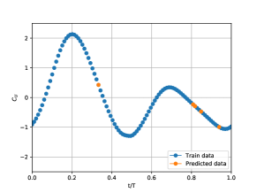
(b)

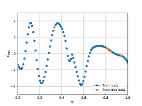
(c)

Figure 4: Time evolution of some reduced coefficients with training points (blue) and test points (orange).

We start to perform a convergence test as the number of snapshots increases. We collect 100, 200 and 400 full order snapshots, each every 0.008 s, 0.004 s and 0.002 s, respectively (i.e. we use an equispaced grid in time), over a cardiac cycle $T=0.8$ s. Fig. 5 shows $L^{2}$-norm relative error $\varepsilon$ for pressure, velocity and WSS fields over time for the three different sampling frequencies. We set $\delta=0.99$ based on the first 90 most energetic POD modes (3 modes for pressure, 15 modes for velocity and 16 modes for WSS). Fig. 5 shows that there is no substantial difference in the errors. Thus, to reduce the computational cost of the offline phase, we will consider 100 snapshots for the results presented from here on.

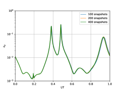
(a)

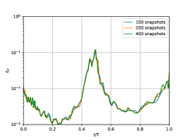
(b)

(c)

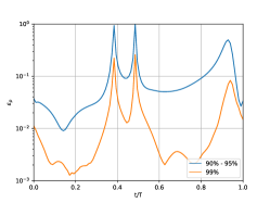
(d)

(e)

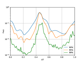
(f)

Figure 5: Time evolution of the relative error $\varepsilon$ varying the number of snapshots (first raw) for LABEL:sub@err_snap:a pressure, LABEL:sub@err_snap:b velocity and LABEL:sub@err_snap:c WSS, and varying the number of modes (second raw) for LABEL:sub@err_mod:d pressure, LABEL:sub@err_mod:e velocity and LABEL:sub@err_mod:f WSS.

Next, we carry out a convergence test as the number of modes increases. We consider three different energy thresholds: $\delta=0.90$ (1 mode for pressure, 3 modes for velocity and 3 modes for WSS), $0.95$ (1 mode for pressure, 5 modes for velocity and 5 modes for WSS), and $0.99$ (3 modes for pressure, 15 modes for velocity and 16 modes for WSS). Of course the pressure error is the same for $\delta=0.90,0.95$ because a single mode is enough to reach $95\%$ of the system energy. From Fig. 5, we observe that all the variables show a monotonic convergence as the number of the modes is increased. For $\delta=0.99$ we obtain time-averaged errors of about 1.7% for the pressure and less than 1% for velocity and WSS.

A qualitative comparison between FOM and ROM simulations is reported in Figs. 6 - 11 for $t/T=0.8$. We display the stenosis and the anastomosis regions that, from the medical viewpoint, are those of major interest because they are modifications with respect to the healthy configuration. As one can see from Figs. 6 - 11, our ROM is able to provide a good reconstruction of velocity and pressure fields, as well as WSS field. Figs. 6 and 7 show the normalized pressure drop $P^{*}=P/P_{max}$ which is a useful indicator in the clinical practice to detect the presence of a stenosis and to measure its severity.

\begin{overpic}[width=138.76157pt]{img/p_FOM_graft} \put(20.0,105.0){FOM} \end{overpic}

(a)

\begin{overpic}[width=138.76157pt]{img/p_ROM_0.99_graft} \put(20.0,105.0){ROM} \end{overpic}

(b)

Figure 6: Comparison between normalized pressure drop $P^{*}=P/P_{max}$ in the anastomosis region computed by the FOM and by the ROM for $t/T=0.8$. We set $\delta=0.99$.

\begin{overpic}[width=138.76157pt]{img/p_FOM_stenosi} \put(20.0,105.0){FOM} \end{overpic}

(a)

\begin{overpic}[width=138.76157pt]{img/p_ROM_0.99_stenosi} \put(20.0,105.0){ROM} \end{overpic}

(b)

Figure 7: Comparison between normalized pressure drop $P^{*}=P/P_{max}$ in the stenosis region computed by the FOM and by the ROM for $t/T=0.8$. We set $\delta=0.99$.

Figs. 8 and 9 report the WSS distribution. As expected, a region of locally high WSS is found near the anastomosis and across the stenosis. It can represent a significant indication for the restenosis process.

\begin{overpic}[width=138.76157pt]{img/WSS_FOM_graft} \put(20.0,105.0){FOM} \end{overpic}

(a)

\begin{overpic}[width=138.76157pt]{img/WSS_ROM_0.99_graft} \put(20.0,105.0){ROM} \end{overpic}

(b)

Figure 8: Comparison between WSS distribution (Pa) in the anastomosis region computed by the FOM and by the ROM for $t/T=0.8$. We set $\delta=0.99$.

\begin{overpic}[width=138.76157pt]{img/WSS_FOM_stenosi} \put(20.0,105.0){FOM} \end{overpic}

(a)

\begin{overpic}[width=138.76157pt]{img/WSS_ROM_0.99_stenosi} \put(20.0,105.0){ROM} \end{overpic}

(b)

Figure 9: Comparison between WSS distribution (Pa) in the stenosis region computed by the FOM and by the ROM for $t/T=0.8$. We set $\delta=0.99$.

Velocity streamlines are depicted in Figs. 10 and 11. The velocity is higher in the LITA because it supplies blood to the entire vessels network, oxygenating LAD and, going up this vessel, LCx too. In Fig. 11, we observe that the velocity is elevated in the stenosis region due to the decreasing diameter. In addition, it can be seen a flow recirculation zone downstream of the stenosis. This phenomenon could favour the deposit of fatty materials on the surface of the lumen, causing the extension of the stenosis.

\begin{overpic}[width=138.76157pt]{img/U_FOM_stream_graft} \put(20.0,105.0){FOM} \end{overpic}

(a)

\begin{overpic}[width=138.76157pt]{img/U_ROM_stream_graft_0.99} \put(20.0,105.0){ROM} \end{overpic}

(b)

Figure 10: Comparison between velocity streamlines (m/s) in the anastomosis region computed by the FOM and by the ROM for $t/T=0.8$. We set $\delta=0.99$.

\begin{overpic}[width=138.76157pt]{img/U_FOM_stream_stenosi} \put(20.0,105.0){FOM} \end{overpic}

(a)

\begin{overpic}[width=138.76157pt]{img/U_ROM_stream_stenosi_0.99} \put(20.0,105.0){ROM} \end{overpic}

(b)

Figure 11: Comparison between velocity streamlines (m/s) in the stenosis region computed by the FOM and by the ROM for $t/T=0.8$. We set $\delta=0.99$.

Finally, we comment on the computational costs. We ran the FOM simulations in parallel using 20 processor cores. The simulations are run on the SISSA HPC cluster Ulysses (200 TFLOPS, 2TB RAM, 7000 cores). Each FOM simulation takes roughly 41 h in terms of wall time, or 820 h in terms of total CPU time (i.e., wall time multiplied by the number of cores). On the other hand, the ROM has been run on an Intel(R) Core(TM) i5-8265U CPU @ 1.60GHz 8GB RAM by using one processor core only. Our ROM approach takes about 10 s for the computation of the reduced coefficients. So we obtain a speed-up of about $3\cdot 10^{5}$.

5 PERSPECTIVES AND CONCLUSIONS

In this work, a non-intrusive data-driven ROM based on POD-ANN approach is developed for fast and reliable numerical simulation of blood flow patterns occurring in a patient-specific coronary system when an isolated stenosis of the LMCA occurs. A CABG performed with the LITA on the LAD is analyzed. The introduction of a patient-specific configuration is an attracting element of this work because it allow to establish a personalized clinical treatment. In addition, it is used a FFD technique, which gives the opportunity to deform directly the mesh and not only the geometry. Furthermore, the combination of ROM, FV technique and neural networks makes this study mathematically appealing.

However, some insights are feasible. Parametric studies involving both physical and geometrical parameters will be performed in Siena et al., 2022. Moreover, one could introduce Windkessel models (Girfoglio et al., 2020, 2021; Fevola et al., 2021) in order to enforce more realistic outflow boundary conditions, which represent a crucial step to obtain meaningful outcomes. In addition, it could be interesting to investigate other ROM frameworks based on other deep learning approaches with the aim to furthermore improve both efficiency and accuracy of the method, such as physics-informed neural network (Chen et al., 2021; Kissas et al., 2020; Demo et al., 2021).

Another important aspect deals with the combination of the ROM framework developed with technological progress through a web interface that would allow real time data to be accessed in hospitals and operating rooms on portable devices. In this scenario, the web server ARGOS (https://argos.sissa.it) has been created, which has the task of proposing a platform to favor a more widespread exploitation of real time computing through a simple "click". ARGOS offers a wide variety of applications related to several problems, implemented by using boh intrusive (RBniCS, ITHACA-FV) and non intrusive (EZyRB, PyDMD) ROM-based softwares developed by SISSA mathLab (https://mathlab.sissa.it/cse-software), and in particular it contains the section ATLAS (https://argos.sissa.it/atlas, see Girfoglio et al. (2021) for further details) focused on the cardiovascular field.

References

- Amoiralis and Nikolos (2008) Amoiralis, E.I., Nikolos, I.K., 2008. Freeform deformation versus B-spline representation in inverse airfoil design. Journal of computing and information science in engineering 8, 024001.
- Ballarin et al. (2016) Ballarin, F., Faggiano, E., Ippolito, S., Manzoni, A., Quarteroni, A., Rozza, G., Scrofani, R., 2016. Fast simulations of patient-specific haemodynamics of coronary artery bypass grafts based on a POD–Galerkin method and a vascular shape parametrization. Journal of computational physics 315, 609–628.
- Ballarin et al. (2017) Ballarin, F., Faggiano, E., Manzoni, A., Quarteroni, A., Rozza, G., Ippolito, S., Antona, C., Scrofani, R., 2017. Numerical modeling of hemodynamics scenarios of patient-specific coronary artery bypass grafts. Biomechanics and modeling in mechanobiology 16, 1373–1399.
- Benner et al. (2015) Benner, P., Gugercin, S., Willcox, K., 2015. A survey of projection-based model reduction methods for parametric dynamical systems. Society for industrial and applied mathematics 57, 483–531.
- Benner et al. (2020) Benner, P., Schilders, W., Grivet-Talocia, S., Quarteroni, A., Rozza, G., Miguel Silveira, L., 2020. Model Order Reduction: Volume 3 Applications. volume 3. De Gruyter.
- Brujic et al. (2002) Brujic, D., Ristic, M., Ainsworth, I., 2002. Measurement-based modification of NURBS surfaces. Computer-aided design 34, 173–183.
- Buoso et al. (2019) Buoso, S., Manzoni, A., Alkadhi, H., Plass, A., Quarteroni, A., Kurtcuoglu, V., 2019. Reduced-order modeling of blood flow for noninvasive functional evaluation of coronary artery disease. Biomechanics and modeling in mechanobiology 18, 1867–1881.
- Burgos et al. (2015) Burgos, M., Lozano, C., Valero, E., 2015. NURBS-based geometry parameterization for aerodynamic shape optimization. Ph.D. thesis. Dissertation, PhD thesis, Universidad Politecnica de Madrid.
- Chen et al. (2021) Chen, W., Wang, Q., Hesthaven, J.S., Zhang, C., 2021. Physics-informed machine learning for reduced-order modeling of nonlinear problems. Journal of computational physics 446, 110666.
- d’Allonnes et al. (2002) d’Allonnes, F.R., Corbineau, H., Le Breton, H., Leclercq, C., Leguerrier, A., Daubert, C., 2002. Isolated left main coronary artery stenosis: long term follow up in 106 patients after surgery. Heart 87, 544–548.
- Demo et al. (2021) Demo, N., Strazzullo, M., Rozza, G., 2021. An extended physics informed neural network for preliminary analysis of parametric optimal control problems. arXiv preprint arXiv:2110.13530 .
- Donadini et al. (2021) Donadini, E., Strazzullo, M., Tezzele, M., Rozza, G., 2021. A data-driven partitioned approach for the resolution of time-dependent optimal control problems with dynamic mode decomposition. arXiv preprint arXiv:2111.13906 .
- Eckart and Young (1936) Eckart, C., Young, G., 1936. The approximation of one matrix by another of lower rank. Psychometrika 1, 211–218.
- Fevola et al. (2021) Fevola, E., Ballarin, F., Jiménez-Juan, L., Fremes, S., Grivet-Talocia, S., Rozza, G., Triverio, P., 2021. An optimal control approach to determine resistance-type boundary conditions from in-vivo data for cardiovascular simulations. arXiv preprint arXiv:2104.13284 .
- Fossan et al. (2021) Fossan, F.E., Müller, L.O., Sturdy, J., Bråten, A.T., Jørgensen, A., Wiseth, R., Hellevik, L.R., 2021. Machine learning augmented reduced-order models for FFR-prediction. Computer methods in applied mechanics and engineering 384, 113892.
- Gaudino et al. (2014) Gaudino, M., Massetti, M., Farina, P., Hanet, C., Etienne, P.Y., Mazza, A., Glineur, D., 2014. Chronic competitive flow from a patent arterial or venous graft to the circumflex system does not impair the long-term patency of internal thoracic artery to left anterior descending grafts in patients with isolated predivisional left main disease: long-term angiographic results of 2 different revascularization strategies. The journal of thoracic and cardiovascular surgery 148, 1856–1859.
- Gharleghi et al. (2020) Gharleghi, R., Samarasinghe, G., Sowmya, A., Beier, S., 2020. Deep learning for time averaged wall shear stress prediction in left main coronary bifurcations. 17th international symposium on biomedical imaging , 1–4.
- Girfoglio et al. (2020) Girfoglio, M., Ballarin, F., Infantino, G., Nicolò, F., Montalto, A., Rozza, G., Scrofani, R., Comisso, M., Musumeci, F., 2020. Non-intrusive PODI-ROM for patient-specific aortic blood flow in presence of a LVAD device. arXiv preprint arXiv:2007.03527 .
- Girfoglio et al. (2021) Girfoglio, M., Scandurra, L., Ballarin, F., Infantino, G., Nicolò, F., Montalto, A., Rozza, G., Scrofani, R., Comisso, M., Musumeci, F., 2021. Non-intrusive data-driven ROM framework for hemodynamics problems. Acta mechanica sinica 37, 1183–1191.
- Goodfellow et al. (2016) Goodfellow, I., Bengio, Y., Courville, A., 2016. Deep learning. Massachusetts institute of technology press.
- Harling et al. (2012) Harling, L., Sepehripour, A.H., Ashrafian, H., Lane, T., Jarral, O., Chikwe, J., Dion, R.A., Athanasiou, T., 2012. Surgical patch angioplasty of the left main coronary artery. European journal of cardio-thoracic surgery 42, 719–727.
- Hesthaven et al. (2016) Hesthaven, J.S., Rozza, G., Stamm, B., et al., 2016. Certified reduced basis methods for parametrized partial differential equations. volume 590. Springer.
- Hesthaven and Ubbiali (2018) Hesthaven, J.S., Ubbiali, S., 2018. Non-intrusive reduced order modeling of nonlinear problems using neural networks. Journal of computational physics 363, 55–78.
- Ishida et al. (2001) Ishida, N., Sakuma, H., Cruz, B.P., Shimono, T., Tokui, T., Yada, I., Takeda, K., Higgins, C.B., 2001. MR flow measurement in the internal mammary artery–to–coronary artery bypass graft: comparison with graft stenosis at radiographic angiography. Radiology 220, 441–447.
- Issa (1986) Issa, R.I., 1986. Solution of the implicitly discretised fluid flow equations by operator-splitting. Journal of computational physics 62, 40–65.
- Keegan et al. (2004) Keegan, J., Gatehouse, P.D., Yang, G.Z., Firmin, D.N., 2004. Spiral phase velocity mapping of left and right coronary artery blood flow: Correction for through-plane motion using selective fat-only excitation. Journal of magnetic resonance omaging 20, 953–960.
- Kissas et al. (2020) Kissas, G., Yang, Y., Hwuang, E., Witschey, W.R., Detre, J.A., Perdikaris, P., 2020. Machine learning in cardiovascular flows modeling: Predicting arterial blood pressure from non-invasive 4D flow MRI data using physics-informed neural networks. Computer methods in applied mechanics and engineering 358, 112623.
- Lamousin and Waggenspack (1994) Lamousin, H.J., Waggenspack, N., 1994. NURBS-based free-form deformations. Graphics and applications 14, 59–65.
- Lassila et al. (2013a) Lassila, T., Manzoni, A., Quarteroni, A., Rozza, G., 2013a. A reduced computational and geometrical framework for inverse problems in hemodynamics. International journal for numerical methods in biomedical engineering 29, 741–776.
- Lassila et al. (2013b) Lassila, T., Manzoni, A., Quarteroni, A., Rozza, G., 2013b. Boundary control and shape optimization for the robust design of bypass anastomoses under uncertainty. Mathematical modelling and numerical analysis 47, 1107–1131.
- Lassila et al. (2011) Lassila, T., Manzoni, A., Rozza, G., 2011. Reduction strategies for shape dependent inverse problems in haemodynamics, in: Conference on System Modeling and Optimization, Springer. pp. 397–406.
- Liang et al. (2020) Liang, L., Mao, W., Sun, W., 2020. A feasibility study of deep learning for predicting hemodynamics of human thoracic aorta. Journal of biomechanics 99, 109544.
- Manzoni et al. (2012a) Manzoni, A., Lassila, T., Quarteroni, A., Rozza, G., 2012a. A reduced-order strategy for solving inverse bayesian shape identification problems in physiological flows, in: Modeling, Simulation and Optimization of Complex Processes. Springer, pp. 145–155.
- Manzoni et al. (2012b) Manzoni, A., Quarteroni, A., Rozza, G., 2012b. Model reduction techniques for fast blood flow simulation in parametrized geometries. International journal for numerical methods in biomedical engineering 28, 604–625.
- Manzoni et al. (2012c) Manzoni, A., Quarteroni, A., Rozza, G., 2012c. Shape optimization for viscous flows by reduced basis methods and free-form deformation. International journal for numerical methods in fluids 70, 646–670.
- Marsden and Esmaily-Moghadam (2015) Marsden, A.L., Esmaily-Moghadam, M., 2015. Multiscale modeling of cardiovascular flows for clinical decision support. Applied mechanics reviews 67, 030804.
- Montana et al. (1989) Montana, D.J., Davis, L., et al., 1989. Training feedforward neural networks using genetic algorithms. International joint conference on artificial intelligence 89, 762–767.
- Pandey et al. (2020) Pandey, R., Kumar, M., Majdoubi, J., Rahimi-Gorji, M., Srivastav, V.K., 2020. A review study on blood in human coronary artery: Numerical approach. Computer methods and programs in biomedicine 187, 105243.
- Papapicco et al. (2021) Papapicco, D., Demo, N., Girfoglio, M., Stabile, G., Rozza, G., 2021. The Neural Network shifted-Proper Orthogonal Decomposition: a Machine Learning Approach for Non-linear Reduction of Hyperbolic Equations. arXiv preprint arXiv:2108.06558 .
- Pichi et al. (2021) Pichi, F., Ballarin, F., Rozza, G., Hesthaven, J.S., 2021. An artificial neural network approach to bifurcating phenomena in computational fluid dynamics. arXiv preprint arXiv:2109.10765 .
- Quarteroni et al. (2015) Quarteroni, A., Manzoni, A., Negri, F., 2015. Reduced basis methods for partial differential equations: an introduction. volume 92. Springer.
- Quarteroni and Rozza (2003) Quarteroni, A., Rozza, G., 2003. Optimal control and shape optimization of aorto-coronaric bypass anastomoses. Mathematical models and methods in applied sciences 13, 1801–1823.
- Rosenblum et al. (2019) Rosenblum, J.M., Binongo, J., Wei, J., Liu, Y., Leshnower, B.G., Chen, E.P., Miller, J.S., Macheers, S.K., Lattouf, O.M., Guyton, R.A., et al., 2019. Priorities in coronary artery bypass grafting: Is midterm survival more dependent on completeness of revascularization or multiple arterial grafts? The journal of thoracic and cardiovascular surgery 161, 2070–2078.
- Rozza (2005) Rozza, G., 2005. On optimization, control and shape design of an arterial bypass. International journal for numerical methods in fluids 47, 1411–1419.
- Rumelhart et al. (1986) Rumelhart, D.E., Hinton, G.E., Williams, R.J., 1986. Learning representations by back-propagating errors. Nature 323, 533–536.
- Scott et al. (2000) Scott, R., Blackstone, E.H., McCarthy, P.M., Lytle, B.W., Loop, F.D., White, J.A., Cosgrove, D.M., 2000. Isolated bypass grafting of the left internal thoracic artery to the left anterior descending coronary artery: late consequences of incomplete revascularization. The journal of thoracic and cardiovascular surgery 120, 173–184.
- Shah et al. (2021) Shah, N.V., Girfoglio, M., Quintela, P., Rozza, G., Lengomin, A., Ballarin, F., Barral, P., 2021. Finite element based model order reduction for parametrized one-way coupled steady state linear thermomechanical problems. arXiv preprint arXiv:2111.08534 .
- Sharma and Sharma (2017) Sharma, S., Sharma, S., 2017. Activation functions in neural networks. Towards data science 6, 310–316.
- Siena et al. (2022) Siena, P., Girfoglio, M., Rozza, G., 2022. Neural network reduced order modelling for patient-specific haemodynamics of coronary artery bypass grafts. In preparation .
- Stabile et al. (2020) Stabile, G., Zancanaro, M., Rozza, G., 2020. Efficient geometrical parametrization for finite-volume-based reduced order methods. International journal for numerical methods in engineering 121, 2655–2682.
- Su et al. (2020) Su, B., Zhang, J.M., Zou, H., Ghista, D., Le, T.T., Chin, C., 2020. Generating wall shear stress for coronary artery in real-time using neural networks: Feasibility and initial results based on idealized models. Computers in biology and medicine 126, 104038.
- Tezzele et al. (2018) Tezzele, M., Ballarin, F., Rozza, G., 2018. Combined parameter and model reduction of cardiovascular problems by means of active subspaces and POD-Galerkin methods, in: Mathematical and numerical modeling of the cardiovascular system and applications. Springer, pp. 185–207.
- Tezzele et al. (2021) Tezzele, M., Demo, N., Mola, A., Rozza, G., 2021. PyGeM: Python geometrical morphing. Software impacts 7, 100047.
- Verim et al. (2015) Verim, S., Öztürk, E., Küçük, U., Kara, K., Sağlam, M., Kardeşoğlu, E., 2015. Cross-sectional area measurement of the coronary arteries using CT angiography at the level of the bifurcation: is there a relationship? Diagnostic and interventional radiology 21, 454.
- Zainib et al. (2020) Zainib, Z., Ballarin, F., Fremes, S., Triverio, P., Jiménez-Juan, L., Rozza, G., 2020. Reduced order methods for parametric optimal flow control in coronary bypass grafts, toward patient-specific data assimilation. International journal for numerical methods in biomedical engineering , e3367.