A Robust Description of Hadronic Decays in Light Vector Mediator Models

Abstract

Abelian $U(1)$ gauge group extensions of the Standard Model represent one of the most minimal approaches to solve some of the most urgent particle physics questions and provide a rich phenomenology in various experimental searches. In this work, we focus on baryophilic vector mediator models in the MeV-to-GeV mass range and, in particular, present, for the first time, gauge vector field decays into almost arbitrary hadronic final states. Using only very little theoretical approximations, we rigorously follow the vector meson dominance theory in our calculations. We study the effect on the total and partial decay widths, the branching ratios, and not least on the present (future) experimental limits (reach) on (for) the mass and couplings of light vector particles in different models. We compare our results to current results in the literature. Our calculations are publicly available in a python package to compute various vector particle decay quantities in order to describe leptonic as well as hadronic decay signatures for experimental searches.

I Introduction

In recent years MeV-to-GeV scale neutral vector mediators have received a lot of attention being the focus of searches in several present and future experimental programs. In part this is because they can be involved in the solution of some unsolved conundrums we face today. They have been evoked in association with dark matter models Pospelov:2007mp ; Kamada:2018zxi ; Plehn:2019jeo ; Borah:2021jzu ; Singirala:2021gok ; Holst:2021lzm ; Batell:2021snh , with the muon anomalous magnetic dipole moment Baek:2001kca ; Pospelov:2008zw , with the MiniBooNE excess of electron like events Bertuzzo:2018itn ; Ballett:2018ynz and to alleviate the reported tension in the Hubble constant Escudero:2019gzq .

Theoretically, these vector bosons appear in connection to extensions of the Standard Model (SM) where the SM gauge group is supplemented by an Abelian $U(1)_{Q}$ symmetry. The new gauge coupling $g_{Q}$, charges ($Q$) and the mass of the vector boson $Z_{Q}$ depend on the particular model realization.

The vector mediator can be secluded, when only kinetic mixing with the photon is allowed, or can enjoy direct gauge couplings to SM fermions. In the former case, generally dubbed dark photon, the mediator couples universally to all SM charged fermions and ignores neutrinos. In the latter case, the gauge boson may not only interact with all SM fermions but additional particles, vector-like under the SM symmetry group but chiral-like under $U(1)_{Q}$. Besides, a judicious choice for the charges is generally required to enforce anomaly cancellation.

One can find many limits on the masses and couplings of these particles in the literature. In Refs. Ilten:2018crw ; Bauer:2018onh limits on a few $U(1)_{Q}$ models for a wide range of masses (from 2 MeV to 90 GeV) were derived or recasted from experimental searches for dark photons. Most of these searches rely on the mediator decays into leptons, either electrons, muons or neutrinos. In some models, the branching ratios into leptons indeed dominate. Nevertheless, for baryophilic vector bosons decays into hadronic final states might have a large share of the total decay width. Especially for a $Z_{Q}$ with a mass in the MeV-to-GeV range, these limits fall in the domain of nonperturbative QCD. Hence, it is important to make sure the hadronic resonances that play an important role in determining the experimental bounds in this region are well described. The main purpose of this paper is to improve this description and provide, for the first time, an almost complete set of $Z_{Q}$ decays into arbitrary leptonic and hadronic final states. This is of consequence as one can, misguided by an incomplete or incorrect theoretical description of the data, exclude regions that are still allowed and perhaps hinder the imminent discovery of a new weak force. Besides, present bounds and future predictions for vector mediator models could, in principle, be complemented by hadronic signature searches.

In order to obtain reliable predictions in this low mass region we use a data driven approach fitting $e^{+}e^{-}$ cross-section data using the meson dominance (VMD) model of chiral perturbation theory. Under this model assumptions we can calculate the decay widths and branching ratios of the new $Z_{Q}$ mediator into hadrons by considering its direct mixing to the dominant vector mesons $\rho$, $\omega$ and $\phi$. A similar approach was also used in Ilten:2018crw ; Bauer:2018onh , but here we improve their implementation in several ways.

We explicitly calculate the $Z_{Q}$ width to specific hadronic final states following the same procedure outlined in Plehn:2019jeo fitting the available $e^{+}e^{-}$ data using IMinuit hans_dembinski_2021_5561211 . Many of those fits are based on state-of-the-art hadronic current parametrizations of $e^{+}e^{-}$ annihilation processes Rodrigo:2001kf ; Czyz:2017veo , and all fits are updated to the most recent data. Once the hadronic currents for numerous mesonic final states are parametrized and the fit values are fixed, we can couple the weak force to all individual currents. We include several new hadronic channels with respect to Ilten:2018crw , especially in the region where there are excited states of the $\rho,\omega,$ and $\phi$ above 1 GeV. The results for the hadronic decays of the new $Z_{Q}$ mediator are provided in the python package DeLiVeR that is available for public use on GitHub at https://github.com/preimitz/DeLiVeR with a jupyter notebook tutorial.

This paper is organized as follows. In section II we introduce a class of baryophilic models that we use throughout the paper. The particular couplings to quarks determines the $Z_{Q}$ decays into light hadrons as described in section III. In section IV we discuss how the description of those decays can be improved compared to previous calculations by using the VMD approach with only very little theoretical assumptions. The impact this different approach has on the hadronic widths, the branching ratios, and on the reach of present and future experimental searches for $Z_{Q}$ vector particles is part of section V. Our conclusion and outlook is presented in section VI.

II General Theoretical Framework

We will consider extensions of the SM where a new vector boson $Z_{Q}$ acquires a mass $m_{Z_{Q}}$ after the spontaneous symmetry breaking of an extra gauged $U(1)_{Q}$ symmetry . As it is well known, even if not present at tree-level, kinetic mixing between two $U(1)$ field strength tensors can be generated at loop-level if there are particles charged under both gauge groups Holdom:1985ag . So we will consider the following renormalizable Lagrangian allowed by the $SU(2)_{L}\times U(1)_{Y}\times U(1)_{Q}$ gauge symmetry

$$\mathcal{L}_{\rm gauge}\supset-\frac{1}{4}\hat{F}_{\mu\nu}\hat{F}^{\mu\nu}-\frac{1}{4}\hat{Z}_{Q\mu\nu}\hat{Z}_{Q}^{\mu\nu}-\frac{\epsilon}{2\cos\theta_{W}}\hat{Z}_{Q\mu\nu}\hat{F}^{\mu\nu},$$ (1)

with a kinetic mixing of the hypercharge and the $Q$-charge field strength tensors, $\hat{F}_{\mu\nu}=\partial_{\mu}\hat{F}_{\nu}-\partial_{\mu}\hat{F}_{\mu}$ and $\hat{Z}_{Q\mu\nu}=\partial_{\mu}\hat{Z}_{Q\nu}-\partial_{\mu}\hat{Z}_{Q\mu}$, respectively. We parameterize this mixing by $\epsilon/(2\cos\theta_{W})$ for convenience.

Considering $\epsilon\ll 1$, we can rotate $\hat{F}$ and $\hat{Z}$ as (see appendix A for details)

$$\hat{F}_{\mu}\to F_{\mu}-\frac{\epsilon}{\cos\theta_{W}}Z_{Q\mu}\quad\quad{\rm and}\quad\quad\hat{Z}_{Q\mu}\to Z_{Q\mu}\,,$$

in order to define gauge bosons with canonical kinetic terms. This rotation will also impact the neutral bosons interaction Lagrangian so that the relevant terms involving the new physical $Z_{Q}$ boson are

$$\mathcal{L}_{\rm int}^{0}\supset e\epsilon J^{\mu}_{\rm em}Z_{Q\mu}-g_{Q}J_{Q}^{\mu}Z_{Q\mu}\,,$$ (2)

where $e=g\sin\theta_{W}$ is the electric charge, $g$ and $g_{Q}$ are, respectively, the $SU(2)_{L}$ and $U(1)_{Q}$ coupling constants and $\theta_{W}$ is the SM weak mixing angle. As usual

$$J^{\mu}_{\rm em}=\sum_{f}\bar{f}\gamma^{\mu}\,q^{f}_{\rm em}\,f\,,$$ (3)

is the SM electromagnetic current, $q^{f}_{\rm em}$ is the fermion $f$ electric charge in units of $e$, and

$$J^{\mu}_{Q}=\sum_{f}\bar{f}\gamma^{\mu}\,q^{f}_{Q}\,f\,,$$ (4)

is the new vector current, with $q^{f}_{Q}$ being the $Q$-charge of fermion $f$. If only the first term is present in eq. (2), i.e. if $q^{f}_{Q}=0$ for all fermions, the boson will couple universally to all charged fermions and we will refer to it as the dark photon $Z_{\gamma}$. We will assume $e\epsilon\ll g_{Q}$, so when charges are present we will neglect the kinetic mixing contribution.

Because our main focus here are the hadronic modes for a light $Z_{Q}$ with $m_{Z_{Q}}$ in the MeV-to-GeV range, we will consider a class of anomaly-free baryophylic models where only three right-handed neutrinos were introduced to the particle content of the SM Araki:2012ip . The symmetry generator for these models can be written as

$$Q=B-x_{e}L_{e}-x_{\mu}L_{\mu}-(3-x_{e}-x_{\mu})L_{\tau}\,,$$ (5)

where $B$ is the baryon number and $L_{e},L_{\mu}$ and $L_{\tau}$ are lepton family number operators. To compare with previous works, we will also present our results for the $B$ model. In table 1, we list the models we will use in this work.

$x_{e}$	$x_{\mu}$	$Q$	$q^{f}_{Q}$
			quarks	$e/\nu_{e}$	$\mu/\nu_{\mu}$	$\tau/\nu_{\tau}$
1	1	$B-L$	$\frac{1}{3}$	-1	-1	-1
3	0	$B-3L_{e}$	$\frac{1}{3}$	-3	0	0
0	3	$B-3L_{\mu}$	$\frac{1}{3}$	0	-3	0
0	0	$B-3L_{\tau}$	$\frac{1}{3}$	0	0	-3
1	0	$B-L_{e}-2L_{\tau}$	$\frac{1}{3}$	-1	0	-2
0	1	$B-L_{\mu}-2L_{\tau}$	$\frac{1}{3}$	0	-1	-2
–	–	$B$	$\frac{1}{3}$	0	0	0

Table 1: Symmetry generators and fermion charges for the models considered in this work.

III On the Decays of $Z_{Q}$

In the mass range of interest of this paper, a $Z_{Q}$ can decay into charged or neutral leptons as well as into light hadrons, if kinematically allowed. In the following, we describe its partial decay widths into these channels.

Leptonic Decays:

The $Z_{Q}$ partial decay width into a pair of leptons is given by

$$\Gamma(Z_{Q}\to\ell\bar{\ell})=\frac{C_{\ell}(g_{Q}q_{Q}^{\ell})^{2}}{12\pi}m_{Z_{Q}}\left(1+2\,\frac{m_{\ell}^{2}}{m_{Z_{Q}}^{2}}\right)\sqrt{1-4\frac{m_{\ell}^{2}}{m_{Z_{Q}}^{2}}}\,,$$ (6)

where $m_{\ell}$ is the lepton mass, $C_{\ell}=1\,(1/2)$ for $\ell=e,\mu$ ($\nu_{e},\nu_{\mu},\nu_{\tau}$), $g_{Q}$ is the $U(1)_{Q}$ gauge coupling and $q_{Q}^{\ell}$ the corresponding lepton charge of the model according to table 1. For the dark photon we have to replace $g_{Q}$ with $e\epsilon$ and $q_{Q}^{\ell}$ with $q_{\rm em}^{\ell}=-1$ for all charged leptons as neutrinos do not couple to $Z_{\gamma}$.

When $m_{Z_{Q}}<2\,m_{e}$, the new boson $Z_{Q}$ can also decay into three photons. The decay width for this process can be found in Seo:2020dtx . Nevertheless, the partial decay width for $Z_{Q}\to 3\gamma$ is negligibly small for the models and mass range of interest in this paper and hence, we refrain from including it into our calculations.

Hadronic Decays:

The region $0.5\lesssim m_{Z_{Q}}/{\rm GeV}\lesssim 2$ is plagued by hadronic resonances and perturbative QCD does not provide a reliable way to evaluate vector boson decays into hadrons, so here one has to, instead, turn to chiral perturbation theory Scherer:2002tk . We will use the so-called vector meson dominance model Sakurai:1960ju ; Kroll:1967it ; Lee:1967iv , which successfully describes $e^{+}e^{-}$ annihilations into hadrons and has been also applied more recently to BSM physics Tulin:2014tya ; Ilten:2018crw , to estimate $Z_{Q}\to\mathcal{H}$, where $\mathcal{H}$ is a hadronic final state made of light quarks, via mixing with QCD vector mesons.

Let’s explain briefly how VMD works to describe low-energy QCD. In a nutshell, in the context of SM interactions, VMD splits the electromagnetic light quarks current into three components, the isospin $I=0,I=1$ and the strange quark currents, and identifies them, respectively, with the vector mesons $\omega,\rho$ and $\phi$ OConnell:1995nse . The same result can be obtained by incorporating dynamical gauge fields $V_{\mu}$ of a local hidden symmetry $U(3)_{V}$ Bando:1984ej ; Fujiwara:1984mp ; Kramer:1984cy ; Bando:1985rf ; Bando:1987br into the chiral Lagrangian Fujiwara:1984mp ; Scherer:2002tk . Linear combinations of these gauge fields will then describe the vector mesons. The vector mesons subsequently interact with other vector mesons $V^{\prime}$ and pseudoscalar mesons $P$ through the anomalous Wess-Zumino-Witten (WZW) $VV^{\prime}P$ interactions Fujiwara:1984mp ; Kramer:1984cy ; Bando:1987br .

With the most prominent example being the SM photon, $U(1)$ gauge symmetric fields, such as $Z_{Q\mu}$, enter this pure QCD Lagrangian as external fields through the covariant derivative of the pseudoscalar Goldstone matrix of the chiral Lagrangian Scherer:2002tk . Additional WZW terms Wess:1971yu ; Witten:1983tw are constructed to fully describe the meson sector such as, for example, the $\pi^{0}\to\gamma\gamma$ decay. Whereas in the low-energy limit those U(1) gauge fields interact directly with the pseudoscalar mesons, they dominantly mix with vector mesons in the hadronic resonance region. Hence, we only have to specify the vector meson-gauge field mixing term. Its most general form is given by

$$\mathcal{L}_{VZ_{Q}}=2\,g_{Q}Z^{\mu}_{Q}{\rm Tr}\left[V_{\mu}Q^{f}\right]\,,$$ (7)

with $V^{\mu}=T^{a}V^{a,\mu}$, where $T^{a}$ are $U(3)$ generators. In our case $Q^{f}$ is a diagonal matrix with entries equal to the $U(1)_{Q}$ charges $q^{u,d,s}_{Q}$. For the dark photon $Z_{\gamma}$ one can simply take $g_{Q}\to e\epsilon$ and $q^{f}_{Q}\to q^{f}_{\rm em}$.

The observed vector mesons of the SM are given by

$$\rho:\;\rho^{\mu}T_{\rho}=\rho^{\mu}\frac{1}{2}{\rm diag}(1,-1,0)\,,$$

$$\omega:\;\omega^{\mu}T_{\omega}=\omega^{\mu}\frac{1}{2}{\rm diag}(1,1,0)\,,$$

$$\phi:\;\phi^{\mu}T_{\phi}=\phi^{\mu}\frac{1}{\sqrt{2}}{\rm diag}(0,0,1)~{}.$$ (8)

Once the vector mediator $Z_{Q}$ has converted into a SM vector meson, the $VV^{\prime}P$ interactions, e.g. the $\rho\omega\pi$ vertex, determine their decays. These interactions are encoded in QCD form-factors $F(q^{2})$. The low-energy limit of chiral perturbation theory is always recovered in the VMD model by making $F(q^{2})\to 1$ for $q^{2}\to 0$.

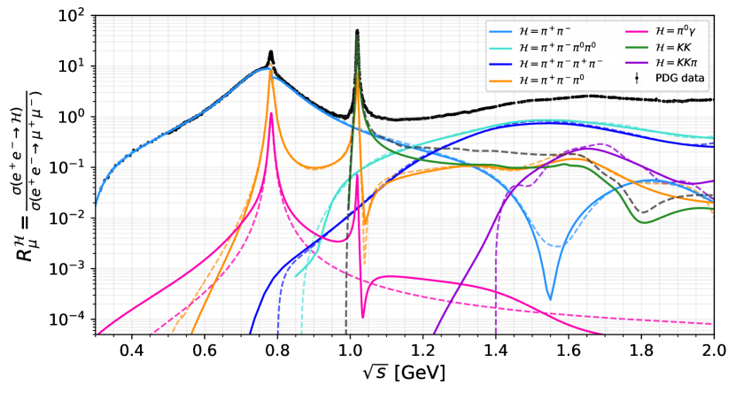
Figure 1: Cross-sections for the dominant $e^{+}e^{-}\to\mathcal{H}$ channels, normalized by the $e^{+}e^{-}\to\mu^{+}\mu^{-}$ cross-section. The solid (dashed) lines indicate results obtained in this work (taken from DarkCast Ilten:2018crw ). The data (black points) was taken from the Particle Data Group compilation (PDG) ParticleDataGroup:2020ssz . See text for discussions on the differences.

All form-factors can be obtained from fits to $e^{+}e^{-}\to\mathcal{H}$ data. The cross-section results are typically displayed as the ratio over the muonic annihilation channel as

$$R_{\mu}^{\mathcal{H}}\equiv\frac{\sigma(e^{+}e^{-}\to\mathcal{H})}{\sigma(e^{+}e^{-}\to\mu^{+}\mu^{-})}\,.$$ (9)

This common rescale of the results for vector portal models is justified since initial state dependencies cancel in the above ratio. As in the dark photon model, the coupling structure is inherited from the SM photon with a proportionality factor $\epsilon$, we can hence model the dark photon decay widths simply by directly rescaling the experimentally known ratios $R_{\mu}^{\mathcal{H}}[\text{\small exp}]\equiv\sigma(e^{+}e^{-}\to\mathcal{H})/\sigma(e^{+}e^{-}\to\mu^{+}\mu^{-})|_{\text{exp}}$ as

$$\Gamma_{Z_{\gamma}\to\mathcal{H}}=\Gamma_{Z_{\gamma}\to\mu^{+}\mu^{-}}R_{\mu}^{\mathcal{H}}[\text{\small exp}].$$ (10)

Although this strategy works well for the dark photon, it cannot be employed anymore when dealing with vector mediators with a coupling structure that is not proportional to the SM photon-quark one. In this scenario the couplings to SM vector mesons need to be determined by eq. (7). For instance, in all the models of interest in this paper, $Z_{Q}$ couples to $B$, so the quark $U(1)_{Q}$ charge matrix takes the form $Q^{f}={\rm diag}(1/3,1/3,1/3)$. In this case the trace for the $\rho$ meson will be zero and hence, only the $\omega$ and $\phi$ mesons will contribute to describe the $Z_{Q}$ decay into hadrons in $R_{\mu}^{\mathcal{H}}$.

Therefore, for generic $U(1)_{Q}$ models, an accurate division of the hadronic channels into their $\rho$, $\omega$ and $\phi$ contributions is of extreme importance in order to obtain the correct description of the hadronic decay widths. In previous studies the VMD approach has been employed with many simplifications and considering a limited number of hadronic channels Ilten:2018crw . These approximations propagate to the width and branching ratio calculations, and can even affect the final experimental bounds in the model parameter space. Next we present a more complete and robust evaluation of various hadronic contributions.

IV Improvements in the Hadronic Calculation

Here we describe the improvements we have implemented in the calculation of the widths and branching ratios of $Z_{\gamma,Q}$ into light hadrons and compare our results with what was used by ref. Ilten:2018crw and is included in the DarkCast code.

Calculation of $\sigma(e^{+}e^{-}\to\mathcal{H})$:

Instead of using the ratio of the total hadronic over muonic annihilations $R_{\mu}^{\mathcal{H}}$ in $e^{+}e^{-}$-processes to estimate the hadronic widths of $Z_{\gamma,Q}$, as in the above mentioned previous work, we have explicitly calculated the individual cross-sections $\sigma(e^{+}e^{-}\to\mathcal{H})$ which enter eq. (9), and contribute to the total hadronic cross-section for the energy range from the pion threshold up to slightly below 2 GeV, using the VMD effective method and experimental data to fit the parameters of the model.

In order to precisely determine the $\rho$-like, $\omega$-like and $\phi$-like contributions to a particular hadronic channel, we parametrize each individual channel playing a part in $e^{+}e^{-}\to{\rm hadrons}$ in terms of its underlying vector meson dominance.

The matrix-element for a given process $e^{+}e^{-}\to\mathcal{H}$ can be written as

$$\mathcal{M}_{e^{+}e^{-}\to\,\mathcal{H}}=\mathscr{L}_{\mu}J^{\mu}_{\mathcal{H}}\,,$$ (11)

where

$$\mathscr{L}_{\mu}=e^{2}\frac{g_{\mu\nu}}{s}\bar{v}(k_{e^{+}})\gamma^{\nu}u(k_{e^{-}})\,,$$

is the leptonic current, $J^{\mu}_{\mathcal{H}}$ is the hadronic current and $\mathcal{H}$ is one of the individual final state configurations $\mathcal{H}=2\pi,3\pi,K\bar{K},...$ we consider here. The hadronic current, which includes a form-factor $F_{\mathcal{H}}$, depending on $\mathcal{H}$, can be written as

$$J^{\mu}_{P_{1}P_{2}} =-(p_{1}-p_{2})^{\mu}F_{P_{1}P_{2}}(q^{2}), \quad J^{\mu}_{P\gamma} =\varepsilon^{\mu\nu\rho\sigma}q_{\nu}\varepsilon_{\gamma,\rho}p_{\gamma,\sigma}F_{P\gamma}(q^{2}),$$ (12)

$$J^{\mu}_{VP} =\varepsilon^{\mu\nu\rho\sigma}q_{\nu}\varepsilon_{V,\rho}p_{P,\sigma}F_{VP}(q^{2}), \quad J^{\mu}_{P_{1}P_{2}P_{3}} =\varepsilon^{\mu\nu\rho\sigma}p_{1,\nu}p_{2,\rho}p_{3,\sigma}F_{P_{1}P_{2}P_{3}}(p_{1},p_{2},p_{3})\,,$$ (13)

where $P_{(1,2,3)},V,\gamma$ indicate, respectively, the presence of a pseudoscalar meson, a vector meson, or a photon in the final state. The corresponding momenta are labeled accordingly. The photon and vector meson polarizations are given by $\varepsilon_{\gamma/V,\mu}$ and $\varepsilon^{\mu\nu\rho\sigma}$ is the antisymmetric Levi-Civita tensor. For the pseudoscalar-pseudoscalar current, the pseudoscalar-photon current and the pseudoscalar-vector current, we have $q=p_{1}+p_{2}$, $q=p_{P}+p_{\gamma}$ and $q=p_{P}+p_{V}$, respectively.

For channels with two pseudoscalars and one vector meson, as in the case of $\omega\pi\pi$ and $\phi\pi\pi$, we refrain from parametrizing the hadronic current in terms of intermediate substructures like $\omega f_{0}\to\omega\pi\pi$ due to dissenting data observations Aubert:2007ef ; Lees:2018dnv . Hence, we assume a point-like interaction and write the hadronic current as

$$J^{\mu}_{VP_{1}P_{2}}=\left(g^{\mu\nu}-\frac{q^{\mu}q^{\nu}}{q^{2}}\right)\varepsilon^{*}_{V,\nu}F_{VP_{1}P_{2}}(q^{2})\,,$$ (14)

with $q=p_{V}+p_{1}+p_{2}$. For channels with more than 3 final states, we directly take expressions from the literature as given in table 3.

In order to calculate the decay width of a vector mediator, we simply replace the leptonic current by the polarization vector of the mediator $L_{\mu}\to\varepsilon_{\mu}(Z_{Q})$ to obtain the matrix element for the decay, so

$$\mathcal{M}_{Z_{Q}\to\mathcal{H}}=\varepsilon_{\mu}(Z_{Q})\sum_{V}r(V)J^{\mu}_{\mathcal{H}}(V)\,,\quad\quad r(V)=\frac{g_{Q}{\rm Tr}\left[T_{V}Q^{f}\right]}{{\rm Tr}\left[T_{V}Q^{\rm em}\right]}\,,$$ (15)

with the factor $r(V)$ rescaling the photon-meson coupling to the mediator-meson coupling with the vector meson resonance $V$, in this case $V=\rho,\omega,\phi$ with generators $T_{V}$ as given in eq. (8).

The dependence on the vector meson resonances $\rho,\omega$ and $\phi$ will appear in the form-factors $F_{\mathcal{H}}$. The dominant vector mesons for a particular channel can be identified using isospin-symmetry assumptions and G-parity conservation. The particular form of these form-factors can be found in Plehn:2019jeo and in appendix B.

In this work, we include the cross-sections for the four most important hadronic contributions close to the $\rho,\omega,$ and $\phi$ masses as well as the $4\pi$ and $KK\pi$ channels that are already part of DarkCast (see table 4), but also consider several new hadronic channels (see table 3) using recent data for the parametrizations. Some of those additional new channels are taken from Plehn:2019jeo , and are complemented by new fits to other channels not considered before in the energy range closer to $\sim 2$ GeV. Table 3 summarizes all additional channels and specifies the vector resonances used in the fit as well as possible final state configurations.

Improvements on the Description of the Dominant Low-Energy Hadronic Modes:

For energy ranges around the ground state vector meson masses, the final states $\pi^{0}\gamma$, $\pi^{+}\pi^{-}$, $\pi^{+}\pi^{-}\pi^{0}$, $KK$ and $KK\pi$ dominate the cross-section. For higher energies we also include the contribution from $e^{+}e^{-}\to 4\pi$. Those channels are very precisely measured and have been also considered by DarkCast. In table 4, we list the assumptions for resonant contributions and its differences to DarkCast, the data used, and references for the parametrizations and fits.

In figure 1, we show our results (solid lines) for these modes and compare them to the state-of-the-art results from DarkCast (dashed lines). Whereas the results are similar around the $\rho$ and $\omega$ masses, channels including the $\phi$ meson give different results. Below, we summarize the main improvements and explain the differences for these channels introduced in our work:

• In the $\pi^{0}\gamma$ channel, besides the $\omega$-like components we include a $\phi$ and a small $\rho$ contribution. The $\phi$, in particular, accounts for a second peak around its mass near 1 GeV (see pink solid line in figure 1) and for the broadening of the $\omega$ peak. Especially in the low-energy limit, below $\simeq 0.6$ GeV, this might have some significant effect if no other hadronic states contribute to the overall decay width of the vector mediator. In the particular case of a $B$ vector boson model, this modification will visibly affect branching ratios, and hence, may modify model limits.

• Regarding the $KK$ channel, we fit both the charged $K^{+}K^{-}$ and neutral $\bar{K}^{0}K^{0}$ components separately, instead of taking $KK=2\;K^{+}K^{-}$ as in the DarkCast code. The latter calculation leads to the overestimation of the total $KK$ cross-section (see dashed green line in figure 1). We also consider the contributions from $\rho$-like, $\omega$-like and $\phi$-like mesons, and not only from $\phi$. The inclusion of these other mesons may have an important impact for models that do not couple to the $\rho$ current, such as the baryophilic $Z_{Q}$ models considered here.

• Finally, the $KK\pi$ channel can be decomposed into three components $\mathcal{H}=K^{0}K^{0}\pi^{0}$, $K^{+}K^{-}\pi^{0}$ and $K^{\pm}K^{0}\pi^{\mp}$. In DarkCast these components are not considered individually. Instead, only the isoscalar component of the $KK\pi$ channel has been taken into account. The isoscalar and isovector contributions can be extracted from the sub-process $e^{+}e^{-}\to{K^{*}(892)K}$, e.g. in the analysis of $e^{+}e^{-}\to K^{\pm}K^{0}\pi^{\mp}$ BaBar:2007ceh . However, this is a two-body process, and therefore has different kinematics compared to a three-body final state. So in order to correctly describe the kinematics of $KK\pi$ we need to make the decomposition into the three final states. Moreover, we take into account the $\rho$-like and $\phi$-like contributions, while DarkCast assigns the whole $[KK\pi]_{I=0}$ as a $\phi$-like channel. The difference between these calculations can be seen in figure 1 (purple lines).

channel	resonances	data	parametrization	fit	possible final states
$\pi\gamma$	$\bm{\rho},\omega,\bm{\omega^{\prime}},\bm{\omega^{\prime\prime}},\bm{\phi}$	SND:2016drm	SND:2016drm	SND:2016drm	$\pi\gamma$
$\pi\pi$	$\rho,\rho^{\prime},...$	KLOE:2008fmq ; BaBar:2009wpw ; BaBar:2012bdw	Czyz:2010hj	Czyz:2010hj	$\pi\pi$
$3\pi$	$\bm{\rho},\bm{\rho}^{\prime\prime},\omega,\omega^{\prime},\omega^{\prime\prime},\phi$	BaBar:2004ytv	Czyz:2005as	Czyz:2005as	$3\pi$
$4\pi$	$\rho,\rho^{\prime},\rho^{\prime\prime},\rho^{\prime\prime\prime}$	BaBar:2012sxt ; BaBar:2017zmc	Czyz:2008kw	Plehn:2019jeo	$4\pi$
$KK$	$\bm{\rho},...,\bm{\omega},...,\phi,...$	CLEO:2005tiu ; Achasov:2000am ; Achasov:2006bv ; Mane:1980ep ; CMD-3:2016nhy ; BaBar:2014uwz ; CMD-2:2008fsu ; BaBar:2013jqz ; BaBar:2015lgl ; Achasov:2016lbc	Czyz:2010hj	Plehn:2019jeo	$KK$
$KK\pi$	$\bm{\rho},\bm{\rho^{\prime}},\bm{\rho^{\prime\prime}},\phi,\phi^{\prime},\phi^{\prime\prime}$	BaBar:2007ceh ; BaBar:2017nrz ; Achasov:2017vaq ; Bisello:1991kd ; Mane:1982si	Plehn:2019jeo	Plehn:2019jeo	$KK\pi$

Table 2: Dominant hadronic processes included in this work as well as in the DarkCast code Ilten:2018crw . We specify the resonances included in the first but not in the latter in boldface  and denote channels where a tower of vector meson resonances was considered with ‘…’. As possible final states we consider low-energy pseudoscalar mesons, $\pi$ and $K$, as well as photons.

channel	resonances	data	parametrization	fit	possible final states
$\eta\gamma$	$\rho,\rho^{\prime},\omega,\phi$	Achasov:2006dv	Achasov:2006dv	Achasov:2006dv	$3\gamma$, $3\pi\gamma$,…
$\eta\pi\pi$	$\rho,\rho^{\prime},\rho^{\prime\prime}$	Achasov:2017kqm ; TheBABAR:2018vvb	Czyz:2013xga	Plehn:2019jeo	$2\pi 2\gamma,5\pi$,…
$\omega\pi\to\pi\pi\gamma$	$\rho,\rho^{\prime},\rho^{\prime\prime}$	Achasov:2016zvn	Achasov:2016zvn	Achasov:2016zvn	$2\pi\gamma$
$\omega\pi\pi$	$\omega^{\prime\prime}$	Akhmetshin:2000wv ; Aubert:2007ef ; Lees:2018dnv	new	new	$5\pi,3\pi\gamma$
$\phi\pi$	$\rho,\rho^{\prime}$	BaBar:2007ceh ; TheBABAR:2017vgl	Plehn:2019jeo	Plehn:2019jeo	$2K\pi$, $4\pi$,…
$\eta^{\prime}\pi\pi$	$\rho^{\prime\prime\prime}$	Aubert:2007ef	Czyz:2013xga	Plehn:2019jeo	$4\pi 2\gamma$,…
$\eta\omega$	$\omega^{\prime},\omega^{\prime\prime}$	Achasov:2016qvd	Plehn:2019jeo	Plehn:2019jeo	$2\pi 2\gamma,6\pi,...$
$\eta\phi$	$\phi^{\prime},\phi^{\prime\prime}$	BaBar:2007ceh ; Achasov:2018ygm	Plehn:2019jeo	Plehn:2019jeo	$KK2\gamma,KK3\pi,...$
$p\bar{p}/n\bar{n}$	$\rho,\rho^{\prime},...,\omega,\omega^{\prime}$,…	Lees:2013ebn ; Ablikim:2015vga ; Pedlar:2005sj ; Delcourt:1979ed ; Castellano:1973wh ; Antonelli:1998fv ; Armstrong:1992wq ; Ambrogiani:1999bh ; Andreotti:2003bt ; Punjabi:2005wq ; Puckett:2011xg ; Gayou:2001qt ; Puckett:2010ac ; Puckett:2017flj ; Pospischil:2001pp ; Plaster:2005cx ; Geis:2008aa ; Andivahis:1994rq	Czyz:2014sha	Plehn:2019jeo	$p\bar{p}/n\bar{n}$
$\phi\pi\pi$	$\phi^{\prime},\phi^{\prime\prime}$	BaBar:2011btv ; Belle:2008kuo	new	new	$KK\pi\pi$
$K^{*}(892)K\pi$	$\rho^{\prime\prime},\phi^{\prime}$	BaBar:2011btv ; BaBar:2017pkz	new	new	$KK\pi\pi$
$6\pi$	$\rho^{\prime\prime\prime}$	BaBar:2006vzy	BaBar:2006vzy	new	$6\pi$

Table 3: Additional processes included in this work that are not present in the DarkCast code Ilten:2018crw . We denoted channels where a tower of vector meson resonances was considered with ‘…’. For the cases where the parametrization and fit are marked as ‘new’, we provide details in appendix B.

Higher resonance effects:

The even more challenging energy region starts above the $\phi$ mass and includes processes involving excited states of the vector mesons $\rho^{\prime},\omega^{\prime},\phi^{\prime}$. The only channel that is rather straightforward to be implemented is the $\rho$ meson dominated $4\pi$ channel with form factors as given in ref. Czyz:2008kw (see navy blue and cyan lines in figure 1). Other processes, especially vector mediator decays to currents involving $\omega$ and $\phi$ contributions, are only poorly described in the literature. We introduce a large amount of new channels in order to accurately describe the region above $\gtrsim 1.5~{}{\mathrm{GeV}}$. To reduce the vast amount of possible final states, we identify common substructures of some channels. For example, the channel $\eta\omega$ can produce $2\pi 2\gamma$ and $6\pi$ final states, whereas $\omega\pi\pi$ can contribute to $5\pi$ and $3\pi\gamma$.

All considered channels and some of their possible final state configurations are listed in table 3. Including additional channels has a significant effect on the total $e^{+}e^{-}\to{\rm hadrons}$ cross-section. As seen in figure 2, the sum of the new contributions to the hadronic cross-section increases up to a level where it contributes as much as the so far considered channels at around $\sqrt{s}\lesssim 2~{}{\mathrm{GeV}}$ (purple line). For center-of-mass energies $\sqrt{s}\gtrsim 1.4~{}{\mathrm{GeV}}$, the $R_{\mu}^{\mathcal{H}}$ line continues to follow the PDG-data to higher energies and captures the effects of excited states of the $\rho,\omega,$ and $\phi$ mesons.

One can also see from figure 2 that the addition of the new channels $\omega\pi\pi$, $6\pi$, $\phi\pi\pi$ and $K^{*}K\pi$ are important especially in the region near $2$ GeV where they dominate. The $\omega\pi\pi$ ($\phi\pi\pi$) channel correspond to a neutral and a charged contribution, $\omega\pi^{0}\pi^{0}$ ($\phi\pi^{0}\pi^{0}$) and $\omega\pi^{+}\pi^{-}$ ($\phi\pi^{+}\pi^{-}$), respectively. The 6$\pi$ channel can also be split into two components, $3(\pi^{+}\pi^{-})$ and $2(\pi^{+}\pi^{-}\pi^{0})$, while the $K^{*}K\pi$ can be split into four components, $K^{*0}K^{\pm}\pi^{\mp}$, $K^{*\pm}K^{0}_{S}\pi^{\mp}$, $K^{*\pm}K^{\mp}\pi^{0}$ decaying into $K^{0}_{S}K^{\pm}\pi^{\mp}\pi^{0}$, and $K^{*0}K^{-}\pi^{+}$ decaying into $K^{+}K^{-}\pi^{+}\pi^{-}$. More details about these channels can be found in appendix B.

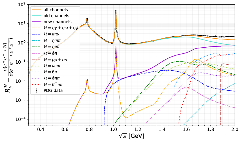
Figure 2: Same as figure 1 but for the new channels included in this work. The dot-dashed lines indicate the hadronic channels already considered in Plehn:2019jeo (but not in Ilten:2018crw ), while the dotted lines indicate channels we have fitted and included here for the first time. The solid lines indicate the total $R_{\mu}^{\mathcal{H}}$ (summed over all hadronic final states) considering: only the channels shown in figure 1 (cyan), only the new channels on table 3 (purple), the sum of all contributions we have calculated (orange).

Final $\rho,\omega$, $\phi$ decomposition

In order to calculate decay widths for arbitrary vector mediator models, it is useful to split up the hadronic current in its $\rho,\omega$ and $\phi$ contributions as given in eq. (7). The quark coupling matrix $Q^{f}$ determines if a certain vector meson contribution is present or absent (${\rm Tr}\left[T_{V}Q^{f}\right]=0$). We can clearly see in figure 3 that the different treatment of the $\pi^{0}\gamma$, $KK$, and $KK\pi$ channels translate into a different $\phi$ contribution above the $\phi$ mass threshold compared to DarkCast. Since we include a lot more channels in the range above $\geq 1.5$ GeV, we also get enhanced $\omega$ and $\rho$ contributions. For vector mediator models with only $\omega$ and $\phi$ couplings, like for example all the $B$-coupled models considered in this paper, this will result in different branching ratios into hadronic final states.

Due to the fact that in the SM the photon mixes with all vector mesons, in the ideal case we expect the $\gamma$-line to follow the PDG data ParticleDataGroup:2020ssz . As seen in figure 3, we can accurately describe the $\gamma$-like until around $\sim 1.7$ GeV. While the $\gamma$-line is almost but not fully overlapping with the $e^{+}e^{-}$-data, we have a more solid description of the separate vector meson contributions due to our approach of summing up all dominant meson channels with subsequent $\rho,\omega,$ and $\phi$ vector meson structures.

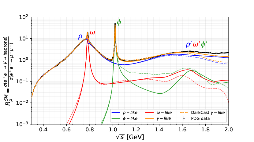
Figure 3: Decomposition of the total hadronic cross-section ratio $R_{\mu}^{\rm SM}\equiv\sum_{\mathcal{H}}R_{\mu}^{\mathcal{H}}$ into $\rho$-, $\omega$- and $\phi$-like contributions for the SM. We also show in orange the total $\gamma$-like contribution. The dashed lines indicate results obtained with the DarkCast code Ilten:2018crw .

Especially in the case of the $\omega$ and $\phi$ contributions, the vector meson contributions differ from the calculations of Ilten:2018crw for vector mediator masses above the $\phi$ meson mass, as well as in the low-energy region of the $\omega$ contribution due to differences in the $\pi^{0}\gamma$ channel. In which way this affects the branching ratios, limits and predictions will be discussed in section V.

Hadron-quark transition

For higher masses than $\gtrsim 1.7$ GeV, we slightly underestimate the $e^{+}e^{-}$ total hadronic cross-section due to missing subdominant multi-meson channels. Although we have included all the available data of the exclusive channels listed in PDG ParticleDataGroup:2020ssz , our results could be improved with better knowledge of the processes and the channels substructures. Also, the inclusion of more data related to final state configurations in the region closer to 2 GeV would improve even more the reach of our $\gamma$-like curve. Possible new channels could be easily added in our approach. Nevertheless, we expect that in that mass range, the annihilation processes slowly transition into perturbative quark production where we have $R_{\mu}^{\mathcal{H}}\to R_{\rm em}=N_{c}\cdot\sum_{f}(q^{f}_{\rm em})^{2}=2$ for the SM with $N_{c}=3$, $q^{u}_{\rm em}=2/3$ and $q^{d,s}_{\rm em}=-1/3$.

In accordance with the PDG ParticleDataGroup:2020ssz , we take

$$R(Q)=R_{\rm em}(1+\delta_{\rm QCD}(Q))\,,$$ (16)

including QCD corrections $\delta_{\rm QCD}(Q)$ that are described in more detail in the QCD review of ParticleDataGroup:2020ssz . As a consequence, due to the lack of sufficient data, the $\gamma$-like curve in figure 3 will be replaced by a perturbative line at $R_{\mu}^{\mathcal{H}}\simeq 2$. For the dark photon model this transition is made at 1.7 GeV, whereas for $B$-coupled models it is at 1.74 GeV. These specific values for the threshold energies were chosen in the intersection between the perturbative quark width, calculated using eq. (16) and the width to muons, and the hadronic width, such that the transition can be done smoothly.

Error estimate:

The uncertainties in our calculation of hadronic decays of light vector mediators emerge from uncertainties from the fits to electron-positron data. As in Ref. Plehn:2019jeo , we define a sub-set of the free fit parameters for each channel and vary their mean values within the uncertainty provided by our IMinuit hans_dembinski_2021_5561211 fit or as stated in the papers. For more details about the uncertainty estimates for the individual channels, we refer to Ref. Plehn:2019jeo . We obtain envelopes around the mean values for the $e^{+}e^{-}$ cross-section data and propagate those parameters to calculate the enveloping curves of the hadronic widths and related quantities.

In Fig. 4 we show in which way this affects the $Z_{B}$ mediator lifetime. As we can see, below the pion threshold, the $Z_{B}$ mediator decays into leptons, which can be calculated perturbatively and, hence, no error bars are included. In the mass region just above the pion threshold up to around 600 MeV the only channel present is $\mathcal{H}=\pi\gamma$. The large uncertainties in this region are justified since no data is available in this mass range as seen in Fig. 16 of appendix B. In an obvious way, our data-driven estimates could be, therefore, improved if new data were available below 600 MeV, in particular for the $\pi\gamma$ channel as it is the dominant hadronic channel in this region for $B$-coupled models. Around and above the $\rho,\omega$ and $\phi$ resonances, the uncertainties lie below the 10% level. The uncertainties will be even smaller for other quantities like the branching ratios as they would affect both nominator and denominator of the ratio. Furthermore, we choose the $B$ model as an example since errors would be, if at all, mostly visible for models that do not couple to the precisely measured $2\pi$ and $4\pi$ currents with small uncertainties as well as to leptons, which would dominate the lifetime computation for masses away from the resonance peaks. Since the theoretical uncertainties are already well below the 10% level for most of the mass range for the lifetime of this model, we refrain from further including them for all other quantities presented in the course of this paper.

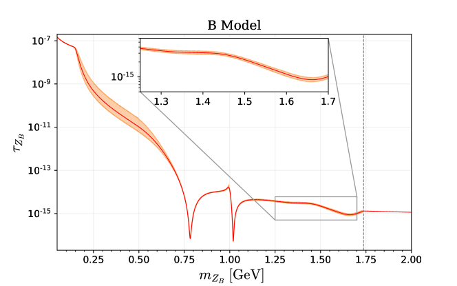
Figure 4: Uncertainty on the $Z_{B}$ mediator lifetime obtained by propagating the cross-section fit envelopes into the hadronic width computation. The red curve is the $Z_{B}$ lifetime evaluated by considering the best fit parameters for each hadronic channel width, while the orange region represents the envelope lifetime uncertainty estimate. The large uncertainties below $\sim 0.6\;{\mathrm{GeV}}$ are caused by the lack of $\pi\gamma$ experimental data in this region. For the regions where data is available, the uncertainties always stay below the 10% level, as we can see in the zoomed in plot. We considered $g_{B}=10^{-4}$ for the lifetime calculation, we remark, however, that the mediator coupling does not affect the uncertainties. The vertical dashed grey line indicates the hadron-quark transition.

V Results and Impact on Present and Future Bounds

We will start this section by presenting the changes in the hadronic decay widths and branching ratios that result from our better assessment of the $Z_{Q}$ decays to light hadrons. After that we will show the consequences on present limits and future experimental sensitivities for a few models.

V.1 Hadronic Decay Widths

In figure 5 we show the total hadronic decay width, normalized to $g_{Q}^{2}\,m_{Z_{Q}}$, as a function of $m_{Z_{Q}}$ for the dark photon (solid blue line, $Z_{Q}=Z_{\gamma}$) and for all the $U(1)_{Q}$ models we discuss in this paper (solid red line). We also show for comparison the results of the previous calculation (dashed lines). The differences between the solid and dashed curves are more sizable in the region $1\lesssim m_{Z_{Q}}/{\rm GeV}\lesssim 1.7$, where we included several new hadronic channels. Close to $1.7\;\rm GeV$ we perform the transition to the perturbative width, which we indicate by splitting the solid curve into another grey curve that represents the hadronic width continuation.

In the region above $1.7\;\rm GeV$, one can see that, for the dark photon case, the width from DarkCast has different features in comparison with the straight perturbative line of our approach. The reason for that is related to the fact that, due to the inclusion of a small number of hadronic channels in Ilten:2018crw , the authors considered the following strategy to reach the total $R_{\mu}^{\rm SM}$ curve: they take their $\gamma$-like curve to be the PDG curve above $1.48\;{\mathrm{GeV}}$ and their calculation below this energy. Then, they define their $\rho$-like curve to be described by the $2\pi$ and $4\pi$ channels below $1.1\;{\mathrm{GeV}}$ and to be the $\gamma$-like curve, with the $\omega$ and $\phi$ contributions subtracted, above it.

On the one hand, the method described above allowed their $\gamma$-like curve to match the $R_{\mu}^{\rm SM}$ experimental calculation. On the other hand, this approximation makes the wrong assumption that all the other neglected hadronic channels contribute as $\rho$ components. As a result, we can see from the figure that right before the transition the red solid line is larger than the dashed one, since baryophilic models do not couple to the $\rho$ current, which means for DarkCast that all the other possible hadronic channels that they did not consider will not couple to the $Z_{Q}$ bosons of these models. We can also see that, for the case of the $B$-coupled models, the dashed line becomes a straight line close to the transition. This behavior is a consequence of the $\omega$ and $\phi$ contributions, that also transition to perturbative values close to $1.6\;{\mathrm{GeV}}$ and $1.7\;{\mathrm{GeV}}$, respectively. However, the red solid line establishes a little bit above the dashed one due to our inclusion of QCD corrections in eq. (16).

Another aspect that is important to highlight is the difference for low energies. The two red lines differ close to $0.6\;{\mathrm{GeV}}$ as a result of the divergences in the calculation of the $\pi\gamma$ channel, as explained in the previous section. This specific channel has a great impact because is the first hadronic channel that couple to the baryophilic model currents. As we will see next, the branching ratios will also modify as a consequence of the above mention disparities.

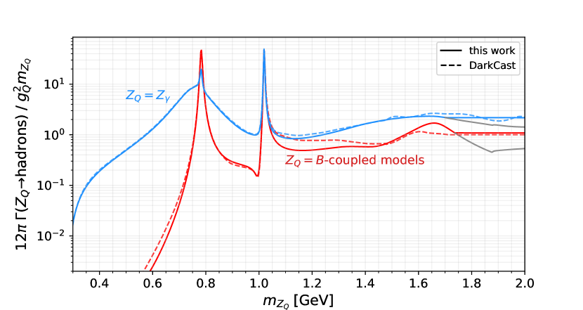
Figure 5: Comparison of the total hadronic width (solid lines) for the dark photon and $B$-coupled (baryophilic) $Z_{Q}$ models with the ones implemented in DarkCast (dashed lines). Around $m_{Z_{Q}}\approx 1.7$ GeV we make the transition to perturbative QCD (see discussion in section IVe).

V.2 Branching Ratios

Now we examine how differences in the hadronic channels affect the branching ratios of the models of interest. In figure 6 in the top panel of each model, we show the branching ratios into $e^{+}e^{-}$ (light blue), $\mu^{+}\mu^{-}$ (blue), neutrinos (green) and hadrons (red) as a function of the mass of the vector boson. The solid (dashed) lines represent the results of our (previous) calculations. In the bottom panel of each plot we show the branching ratio difference between the two calculations.

We show, for reference, the $Z_{\gamma}$ case as well as the pure $Z_{B}$. In the $Z_{\gamma}$ case, DarkCast predicts a larger branching ratio into hadrons than us in the range $0.25\lesssim m_{Z_{\gamma}}/{\rm GeV}\lesssim 1.8$, but the difference is always less than 5%. The discrepancy between the two calculations for $Z_{B}$ is, on the other hand, more visible for $0.2\lesssim m_{Z_{B}}/{\rm GeV}\lesssim 0.4$ because the previous calculation underestimates the $\pi^{0}\gamma$ contribution (see section IV b). In this region, the difference can be as large as $\sim$ 30%. In spite of the fact that for larger values of $m_{Z_{B}}$ the hadronic branching ratios seem to coincide, we see in the left panel of figure 7 that the contributions of each hadronic mode is quite different. For instance, our calculation predicts a much smaller (larger) contribution of the $KK$ (3$\pi$) final state in the region $1.0\lesssim m_{Z_{B}}/{\rm GeV}\lesssim 1.5$.

For the $B-L$, $B-L_{\mu}-2L_{\tau}$, $B-3L_{e}$ and $B-3L_{\tau}$ models , the hadronic contribution to the branching ratio in the region $1.0\lesssim m_{Z_{Q}}/{\rm GeV}\lesssim 1.75$ is sometimes overestimated (due to $KK$ mode) sometimes underestimated (due to higher resonances) by DarkCast, generally influencing the charged lepton and neutrino decay contributions by a few to almost 10% for some values of $m_{Z_{Q}}$ in some of the models. We illustrate these changes in the contributions of the hadronic final states for these models showing them explicitly for the $B-L$ model in the right panel of figure 7.

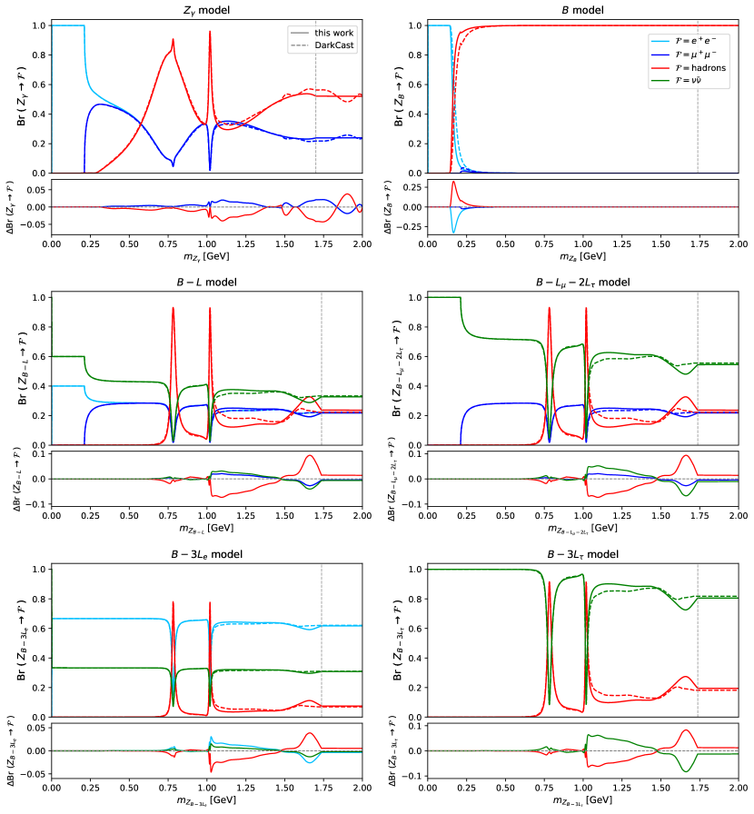
Figure 6: Comparison of the leptonic and hadronic branching ratios (solid lines) with the ones from DarkCast (dashed lines) for some chosen models. The vertical dashed gray line indicates the transition from non-perturbative to perturbative calculations as described in the text. In the lower panel of each figure we show the deviation $\Delta\rm Br$, i.e. our branching ratio minus the DarkCast one.

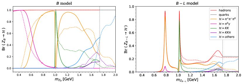
Figure 7: Comparison of the individual contributions to the total hadronic branching ratio between our calculations (solid lines) and DarkCast (dashed lines) for the $B$ (left panel) and $B-L$ (right panel) models. The individual branching ratios for the other $B$-coupled models behave in a similar way to the $B-L$ model. The vertical dashed gray line indicates the transition from non-perturbative to perturbative calculations as described in the text.

V.3 Repercussions on Current Limits and Future Sensitivities

To discuss the effect of our reevaluation of the light hadron contributions to $Z_{Q}$ decays on experimental limits for these models in the range $100\,{\rm MeV}\leq m_{Z_{Q}}\leq 2\,{\rm GeV}$, we have implemented the results of our calculations in the DarkCast and FORESEE codes. DarkCast is a code that recasts experimental limits on dark photon searches to obtain limits on vector boson mediators with couplings to SM fermions. See Ref. Ilten:2018crw for more details on the recasting procedure for the different types of experimental data we have used to obtain the limits presented here. FORESEE (FORward Experiment SEnsitivity Estimator) is a package that can be used to calculate the expected sensitivity for BSM physics of future experiments placed in the forward direction far from the proton-proton interaction point at the LHC. See Ref. Kling:2021fwx for more information on the code.

V.3.1 Current Experimental Limits

To obtain the exclusion regions in the $g_{Q}\times m_{Z_{Q}}$ plane for the various models of interest, we consider the following experimental searches:

1. $Z_{Q}$ produced in the electron fixed target experiments APEX APEX:2011dww and A1 A1:2011yso ; Merkel:2014avp by Bremsstrahlung followed by the prompt decay $Z_{Q}\to e^{+}e^{-}$ NA64:2016oww ; NA64:2017vtt ; Banerjee:2019pds ; and in NA64 followed by the prompt decay $Z_{Q}\to$ invisible ($\nu\bar{\nu}$);

2. $Z_{Q}$ produced via $\pi^{0}\to\gamma Z_{Q}$ in the proton beam dump experiments LSND LSND:1997vqj ; Bauer:2018onh , PS191 Bernardi:1985ny and NuCal Blumlein:1991xh as well as via $\eta\to\gamma Z_{Q}$ in CHARM CHARM:1985anb and via proton Bremsstrahlung in NuCal Blumlein:1990ay , all of them followed by $Z_{Q}\to e^{+}e^{-}$;

3. $Z_{Q}$ produced in the electron beam dump experiment E137 followed by $Z_{Q}\to e^{+}e^{-}$ Bjorken:2009mm ; Andreas:2012mt ;

4. $Z_{Q}$ produced by radiative return in the $e^{+}e^{-}$ annihilation experiments BESIII, BaBar and KLOE or by muon Breemstrahlung in Belle-II. In BaBar, one searches for the decay modes $Z_{Q}\to e^{+}e^{-},\,\mu^{+}\mu^{-}$ BaBar:2014zli and $Z_{Q}\to$ invisible ($\nu\bar{\nu}$) BaBar:2017tiz , in BESSIII for the decay modes $Z_{Q}\to e^{+}e^{-},\,\mu^{+}\mu^{-}$ BESIII:2017fwv and in KLOE for the decay modes $Z_{Q}\to e^{+}e^{-}$ Anastasi:2015qla and $Z_{Q}\to\mu^{+}\mu^{-}$ KLOE-2:2014qxg ; KLOE-2:2018kqf . For KLOE we also use data for the search $\phi\to\eta Z_{Q}\,,Z_{Q}\to e^{+}e^{-}$ KLOE-2:2012lii . In Belle-II, one searches for $Z_{Q}\to$ invisible ($\nu\bar{\nu}$) Belle-II:2019qfb ;

5. $Z_{Q}$ produced in pp collisions at the LHCb experiment either by meson decays or the Drell-Yan mechanism with the subsequent displaced or prompt decay $Z_{Q}\to\mu^{+}\mu^{-}$ LHCb:2017trq ; LHCb:2019vmc ;

6. $Z_{Q}$ produced in kaon decay experiments via $\pi^{0}\to\gamma Z_{Q}$ followed by the prompt decay $Z_{Q}\to e^{+}e^{-}$ at NA48/2 NA482:2015wmo or by $Z_{Q}\to$ invisible ($\nu\bar{\nu}$) at NA62 NA62:2019meo .

Figure 8: In blue the excluded regions in the plane $g_{B}\times m_{Z_{B}}$ we obtained using data from the electron Bremsstrahlung experiments APEX APEX:2011dww and A1 A1:2011yso ; Merkel:2014avp , the proton beam dump experiments PS191 Bernardi:1985ny , NuCal Blumlein:1990ay ; Blumlein:1991xh and CHARM CHARM:1985anb , the electron beam dump experiment E137 Bjorken:2009mm ; Andreas:2012mt , the $e^{+}e^{-}$ annihilation experiments BaBar BaBar:2014zli and KLOE Anastasi:2015qla ; KLOE-2:2012lii , the LHCb experiment LHCb:2017trq ; LHCb:2019vmc , NA48 NA482:2015wmo and LSND LSND:1997vqj ; Bauer:2018onh . In gray the region excluded by the previous calculation Ilten:2018crw , but still allowed by this work. We also show the limits from $B\to KZ_{B}$, $K^{\pm}\to\pi^{\pm}Z_{B}$ and $Z\to\gamma Z_{B}$ taken from Dror:2017ehi for completeness, where the dashed lines represent current bounds and the dotted lines future predictions.

We start by presenting the differences on the limits for the $U(1)_{B}$ model as it highlights the consequences of the improvements of our calculations. In all the plots in blue (green) we show the exclusion regions for $Z_{Q}$ decaying to $e^{+}e^{-}$ and $\mu^{+}\mu^{-}$ pairs (neutrinos). In figure 8 we show in blue the recasted limits for various experiments using our calculations. In gray we can see an extra region that would be excluded by DarkCast, but not by this work. This is particularly visible for $0.2\lesssim m_{Z_{B}}/{\rm GeV}\lesssim 0.4$ where the underestimation of the $\pi^{0}\gamma$ contribution in the previous calculation yields to an enhanced $Z_{B}\to e^{+}e^{-}$ signal prediction. There are also regions where our calculation results in an increase of the exclusion bounds. For instance, we show in figure 8 in gray the contour for the NuCal limits obtained with DarkCast. As one can see, there is a region previously allowed that we can exclude now. This effect is also a consequence of the difference in the lifetime calculation, that is more prominent for the $B$ model, and has a deep impact specially for beam-dump experiments.

There are, however, two caveats here. The first is the fact that the model is anomalous. As it has been shown in Ref. Dror:2017ehi ; Dror:2017nsg light vectors coupled to SM particles and non-conserved currents enhance the rate of meson decays such as $B\to KZ_{B}$ and $K^{\pm}\to\pi^{\pm}Z_{B}$ as well as the Z boson decay $Z\to\gamma Z_{B}$. Those limits mostly lie in areas that have been covered by LHCb with the exception of filling unconstrained areas in the vector meson resonance region. Furthermore, the future $B\to KZ_{B}$ prediction is expected to cover a sizable part of the region $0.5~{}{\rm GeV}\lesssim m_{Z_{B}}$. The second is related to the coupling to leptons, as for all experimental limits the light vector boson is supposed to decay to $e^{+}e^{-}$ and/or $\mu^{+}\mu^{-}$ (BaBar and LHCb). Although $Z_{B}$ does not couple directly to charged leptons, there is a one-loop induced kinetic mixing between $Z_{B}$ and the photon Carone:1994aa . However, the magnitude of this coupling will depends on the choice of the renormalization scale so it cannot be determined unambiguously. In the DarkCast code, which we use, it is taken to be simply $eg_{B}/(4\pi)^{2}$, so the limits involving this coupling to charged leptons have to be regarded with caution.

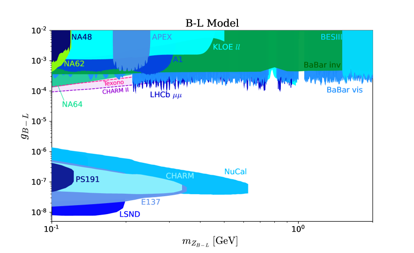
Figure 9: Same as figure 8 but for the $B-L$ model. In blue (green) the excluded regions for $Z_{B-L}$ decaying to charged lepton ($\nu\bar{\nu}$) pairs. Beside the data already included in figure 8, here we also include data from KLOE in the $\mu^{+}\mu^{-}$ final state KLOE-2:2014qxg ; KLOE-2:2018kqf , from BaBar BaBar:2017tiz , NA62 NA62:2019meo and NA64 NA64:2016oww ; NA64:2017vtt ; Banerjee:2019pds invisible searches, and from BESIII BESIII:2017fwv . We also show with dashed lines the limits from the neutrino experiments Texono TEXONO:2009knm (red) and CHARM-II GEIREGAT1990271 (purple) that were taken from Bauer:2018onh .

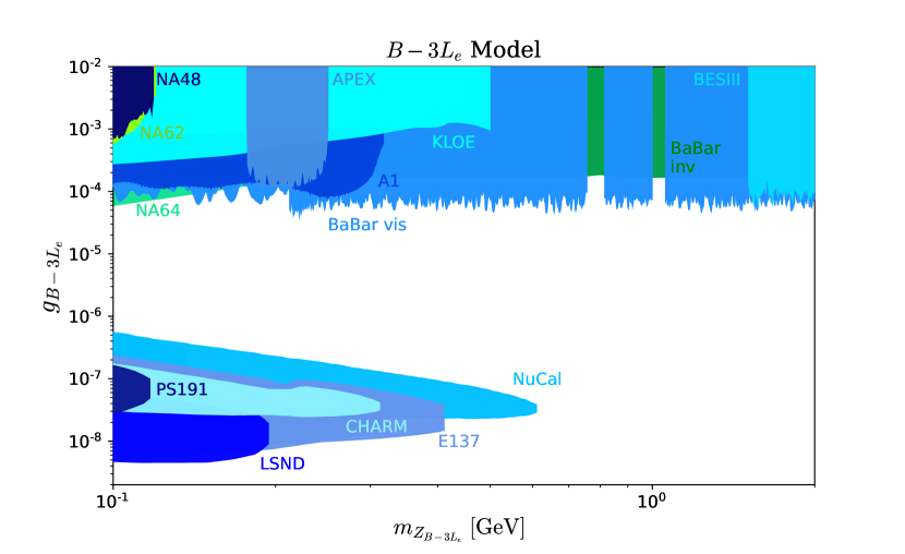
Figure 10: Similar to figure 9 but for the $B-3L_{e}$ model. Here there is no contribution from the LHCb experiment or from KLOE due to the absence of muon couplings.

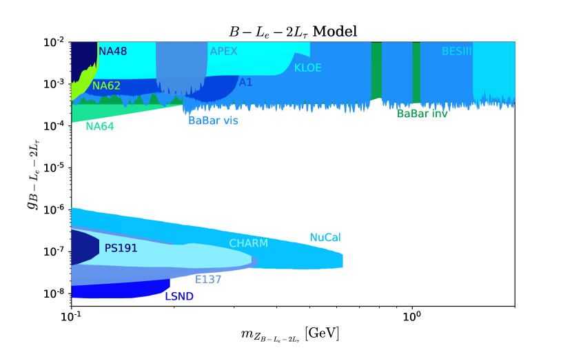
Figure 11: Similar to figure 10 but for the $B-L_{e}-2L_{\tau}$ model.

Next we show the exclusion regions for some of the models we have considered. Although in the case of current limits, the differences caused by our calculations are not very visible in the combined plot, they will affect the sensitivity of future experiments as we will see shortly. In figure 9 we show the exclusion region for $Z_{B-L}$ in the plane $g_{B-L}\times m_{Z_{B-L}}$. Here the differences are small as they practically do not affect $Z_{B-L}\to e^{+}e^{-},\,\mu^{+}\mu^{-}$ and $\bar{\nu}\nu$. However, since this model is of great interest and we have some recent data from LHCb, NA62 and NA64, we decided to present here. We also include for completeness the limits from the neutrino experiments Texono TEXONO:2009knm ; Lindner:2018kjo ; Bilmis:2015lja and CHARM-II GEIREGAT1990271 ; Lindner:2018kjo ; Bilmis:2015lja that were taken from Bauer:2018onh . These limits do not depend on leptonic decays and therefore are independent of the hadronic branching ratios. We do not show the limit from the Borexino Bellini:2011rx ; Harnik:2012ni ; Amaral:2020tga neutrino experiment since the NA64 and CHARM-II limits cover it in the mass range considered in this study. In figure 10 we show the exclusion region for $Z_{B-3L_{e}}$ which is similar but does not contain the constraints from LHCb, and KLOE in the $\mu^{+}\mu^{-}$ final state.

Finally, in figure 11 we show the limits for the $B-L_{e}-2L_{\tau}$ model. The $B-3L_{\mu}$ and $B-L_{\mu}-2L_{\tau}$ models only have bounds from LHCb (prompt), NA62 and Belle-II, while the $B-3L_{\tau}$ model only has bounds from NA62. We do not show them here but refer to Bauer:2020itv for a comprehensive analysis of $B-3L_{i}$ models. Note that all experimental searches reported here look for either leptonic or invisible (neutrino) decays of the vector mediator. Hadronic decays, however, especially close to the vector resonances, could in general be probed.

V.3.2 Future Experimental Sensitivities

Here we discuss how our better assessment of the $Z_{Q}$ decay to light hadrons can affect the sensitivity of various high intensity frontier experiments that can probe them in the near future.

The ForwArd Search ExpeRiment (FASER) is a relatively small cylindrical detector located along the LHC beam axis at approximately 480 m downstream of the ATLAS detector interaction point. The aim is to search for long lived particles profiting of the luminosity and boost of the LHC beam. There are two proposed phases for FASER. In the first phase, named FASER, the detector will be 1.5 m long with a diameter of 20 cm and will operate from 2022 to 2024 FASER:2021ljd , being exposed to an expected integrated luminosity of 150 fb^-1 FASER:2018eoc . In the second phase, named FASER 2, the detector will be 5 m long with a diameter of 2 m and is expected to take data in the high luminosity LHC era, being exposed to an integrated luminosity of 3 ab^-1. Dark photons can be produced by meson decays, $pp\to Z_{\gamma}pp$ (Bremsstrahlung) as well as by direct production in hard scattering. It is important to highlight that, in contrast to the majority of current experimental searches, that rely on leptonic decay signals, the FASER detector will also be sensitive to hadronic final states. Hence, it is crucial to provide a correct hadronic description in order to precisely compute the experiment expected sensitivity.

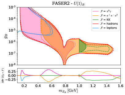
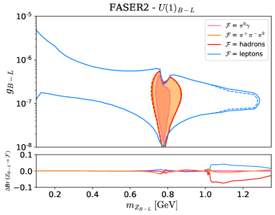
Figure 12: Expected sensitivity for the $B$ (left panel) and $B-L$ (right panel) models for FASER2 using our calculations for the branching fractions implemented in the FORESEE code. The various final state contributions are highlighted by different colors as in figure 7: $\pi\gamma$ (pink), $3\pi$ (orange), $KK$ (green) and leptons (blue). The dashed lines, using the same color scheme, show the results using the FORESEE code and DarkCast branching ratios. In the bottom panels we also show for each model the difference of the branching ratio between our calculation and DarkCast.

In figure 12 we show the sensitivity for the $B$ (left panel) and $B-L$ (right panel) models expected for FASER 2 using the FORESEE code Kling:2021fwx with the implementation of the branching fractions we have calculated. We highlight on these figures the various final state signal contributions by using different colors: $\pi\gamma$ (pink), $3\pi$ (orange), $KK$ (green) and leptons (blue). The dashed lines using the same color scheme are the DarkCast predictions for each mode. We also show in the lower part of these plots the difference of the branching ratio between our calculation and DarkCast. Here we can appreciate that although the final sensitive regions do not differ very much from the one predicted by the previous calculation, the contributions from the different final states are not the same.

The proposed fixed target facility to Search for Hidden Particles (SHiP) at the CERN SPS 400 GeV proton beam Alekhin:2015byh is also able to search for dark photons, as well as other vector gauge bosons that couple to the gauged baryon number B, in the GeV mass range. It is expected to receive a flux of $2\times 10^{20}$ protons on target in 5 years. The beam will hit a Molybdenum and Tungsten target, followed by a hadron stopper and by a system of magnets to sweep muons away. The detector consists of a long decay volume that starts at about 60 m downstream from the primary target and is about 50 m long followed by a tracking system to identify the decay products of the hidden particles, for more details see Bonivento:2013jag . At SHiP dark photons can be produced by meson decays, Bremsstrahlung and QCD. By recasting the projected constraints for the dark photon model from Bremsstrahlung production given in figure 2.6 of ref. Alekhin:2015byh we compute the sensitivity of other models.

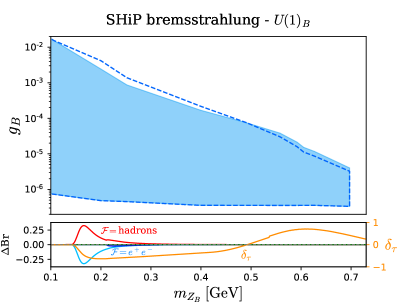
Figure 13: Expected sensitivity for the $B$ (left panel) and $B-L_{e}-2L_{\tau}$ (right panel) models for SHiP Bremsstrahlung production from our calculation (solid light blue) and DarkCast (dashed lines). In the bottom panels we show for each model the difference of the branching ratio between the two calculations, and for the $B$ model the corresponding difference in lifetime ($\delta_{\tau}$, in orange).

In figure 13 we compare the sensitivity of the SHiP Bremsstrahlung production search for $Z_{B}$ (left panel) and $Z_{B-L_{e}-2L_{\tau}}$ (right panel) predicted by us (solid light blue) and DarkCast (dashed line). On the bottom panels we show again the difference in the predicted branching ratios between the two calculations. For the $B$ model we also show the corresponding difference in lifetime ($\delta_{\tau}$, in orange). If the lifetime is too short $Z_{B}$ will not be able to reach the detector. So the difference with DarkCast comes from the smaller lifetime (for $m_{Z_{B}}\lesssim 0.5$ GeV) and larger lifetime (for $m_{Z_{B}}\gtrsim 0.5$ GeV) predicted by our calculation. In the case of the $B-L_{e}-2L_{\tau}$ model, the predicted SHiP sensitivity stops earlier, at a mass of about 1.6 GeV, due to the increase of the hadronic final state modes above this mass.

Belle-II is a high luminosity B-factory experiment at the SuperKEKB $e^{+}e^{-}$ collider in Japan operating at center of mass energies in the region of the $\Upsilon$ resonances. It can search for $Z_{\gamma}$ produced via the initial-state radiation (ISR) reaction $e^{+}e^{-}\to\gamma_{\rm ISR}\,Z_{\gamma}$, with $Z_{\gamma}$ decaying to all kinetically accessible light charged states. The signature for a dark photon promptly decaying into leptons is a peak in the distribution of the reconstructed mass of the final lepton pair. We use the projected sensitivity for the visible decay modes $Z_{\gamma}\to e^{+}e^{-},\mu^{+}\mu^{-}$ from Fig. 211 of ref. Belle-II:2018jsg , corresponding to a total integrated luminosity of 50 ab^-1, to recast Belle-II dark photon limit to other models (visible searches). This experiment can also look for $e^{+}e^{-}\to\gamma_{\rm ISR}\,Z_{Q},Z_{Q}\to$ invisible, by searching for mono-energetic ISR single photons. We use their projected sensitivity for this invisible decay mode taken from figure 209 of ref. Belle-II:2018jsg to calculate the sensitivity of models where $Z_{Q}\to\nu\bar{\nu}$ can occur (invisible searches).

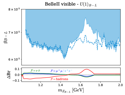
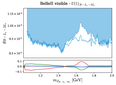
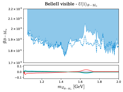
Figure 14: Similar to figure 13 but for Belle II visible searches and for the following models: $B-L$ (top left panel), $B-L_{e}-2L_{\tau}$ (top right panel) and $B-3L_{e}$ (bottom panel). In solid light blue (dashed line) we show our (DarkCast) results.

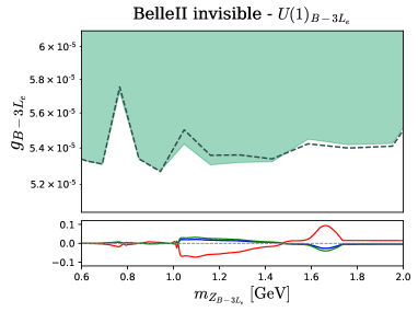
Figure 15: Expected sensitivity for the $B-L$ (left panel) and $B-3L_{e}$ (right panel) models for Belle II invisible searches according to our calculation (solid green) and DarkCast (dashed lines). In the bottom panels we show for each model the difference of the branching ratio between the two calculations. The 11 data points shown in the figure are taken from Belle-II:2018jsg .

In figure 14 we display the predicted sensitivity for Belle II (visible searches) for the $B-L$ (top left panel), $B-L_{e}-2L_{\tau}$ (top right panel) and $B-3L_{e}$ (bottom panel) models. We predict (solid light blue) for all these models a loss of sensitivity for vector boson masses between 1.5 GeV and 1.8 GeV, due to an increase of hadronic final states (and consequent decrease of leptonic ones) in this mass window. We also predict a slight increase in sensitivity in other mass regions.

Finally, in figure 15 we can see the expected sensitivity for Belle II invisible searches for the $B-L$ (left panel) and $B-3L_{e}$ (right panel) models. Here again the decrease (increase) of the hadronic final state contributions in certain mass regions, respond for the increase (decrease) of sensitivity of Belle II in the invisible mode according to our assessment.

VI Final Conclusions and Outlook

In this paper we present an improved calculation of the decay width and branching ratios for baryophilic vector boson mediators $Z_{Q}$, associated with a new U(1)_Q gauge symmetry and having a mass in the MeV-to-GeV range, providing for the first time an almost complete set of $Z_{Q}$ decays into arbitrary leptonic and hadronic final states.

This is relevant as one can, misguided by an incomplete or incorrect theoretical description of the data, exclude regions that are still allowed and perhaps hinder the imminent discovery of a new weak force in this mass region by future experiments. Furthermore, present and future experiments could, in principle, look for hadronic signatures of these states, in particular close to hadronic resonances.

We use a data driven approach fitting $e^{+}e^{-}$ cross-sections from various experiments and the meson dominance model of chiral perturbation theory to derive reliable predictions. The VMD model allows us to calculate the decay widths and branching ratios of the new $Z_{Q}$ into light hadrons by considering its direct mixing to the dominant vector mesons $\rho,\omega$ and $\phi$. This was done before in Ilten:2018crw but we improve their calculation in various ways.

We have updated to the most recent $e^{+}e^{-}$ data (see tables 4 and 3), we included a more complete description of the dominant vector meson contributions, we corrected the $KK$ ($\pi^{0}\gamma$) contribution that was overestimated (underestimated) before, we have considered the individual contributions to the $KK\pi$ channel correctly describing the final state kinematics and we included several new hadronic channels (see table 3), in particular, above 1 GeV. See appendix B for further details on the calculations for old and new channels.

We discussed the impact of our new calculation on the hadronic decay widths and branching ratios of some baryophilic $Z_{Q}$ models as well as on the current experimental limits on the plane $g_{Q}\times m_{{Z}_{Q}}$ for these models.

We also show how some future experiments (FASER 2, SHiP, Belle II) can have their sensitivities affected by our better assessment of the $Z_{Q}$ hadronic modes.

The results for hadronic decays of any new $Z_{Q}$ mediator in the MeV-to-GeV mass range are provided for public use in the python package DeLiVeR that is available on GitHub at https://github.com/preimitz/DeLiVeR with a jupyter notebook tutorial. See appendix C for some information of what can be found in our hadronic decay package.

Appendix A $Z_{Q}$: kinetic mixing, mass mixing and couplings to SM fermions

The most general Lagrangian that describes our model includes the kinetic mixing between $U(1)_{Y}$ and $U(1)_{Q}$, direct couplings of the new $U(1)_{Q}$ boson to SM fermions and mass mixing between $Z$ and $Z_{Q}$. The first relevant term involving the neutral gauge bosons is

$$\mathcal{L}^{0}_{\rm gauge}=-\frac{1}{4}\hat{F}_{\mu\nu}\hat{F}^{\mu\nu}-\frac{1}{4}\hat{Z}_{Q\mu\nu}\hat{Z}_{Q}^{\mu\nu}-\frac{\epsilon}{2\cos\theta_{W}}\hat{Z}_{Q\mu\nu}\hat{F}^{\mu\nu},$$ (17)

which describes the gauge fields $\hat{F}$ and $\hat{Z}$ mixing via the coupling of their field strength tensors $\hat{F}^{\mu\nu}$ and $\hat{Z}^{\mu\nu}_{Q}$. To bring this term to the canonical form we perform the GL(2,R) rotation

$$\begin{pmatrix}\hat{Z}_{Q}^{\mu}\\ \hat{F}^{\mu}\end{pmatrix}=\begin{pmatrix}\frac{1}{\sqrt{1-(\epsilon/c_{W})^{2}}}&0\\ -\frac{\epsilon/c_{W}}{\sqrt{1-(\epsilon/c_{W})^{2}}}&1\end{pmatrix}\begin{pmatrix}\tilde{Z}_{Q}^{\mu}\\ F^{\mu}\end{pmatrix}\,,$$ (18)

where $c_{W}=\cos\theta_{W}$, so that for $\epsilon\ll 1$ the fields are redefined as

$$\hat{Z}^{\mu}_{Q}\to\tilde{Z}^{\mu}_{Q}\,,\quad\quad\hat{F}^{\mu}\to F^{\mu}-\frac{\epsilon}{c_{W}}\tilde{Z}^{\mu}_{Q}\,.$$ (19)

The interactions of the $SU(2)_{L}$, $U(1)_{Y}$ and the new $U(1)_{Q}$ gauge bosons, $\hat{W}^{1,2,3}$, $\hat{F}$ and $\hat{Z}_{Q}$, respectively, with the SM chiral fermions are described by

$$\mathcal{L}_{\rm int}=\sum_{f}i\bar{f}\gamma^{\mu}D_{\mu}f,$$ (20)

in terms of the covariant derivative

$$D_{\mu}\equiv\partial_{\mu}+ig\sum_{a=1}^{3}\frac{\tau^{a}}{2}\hat{W}^{a}_{\mu}+ig^{\prime}Q_{Y}\hat{F}_{\mu}+ig_{Q}Q_{Q}\hat{Z}_{Q\mu}\,,$$

where $g$ ($\tau^{a}/2$), $g^{\prime}$ ($Q_{Y}$) and $g_{Q}$ ($Q_{Q}$) are the $SU(2)_{L}$, $U(1)_{Y}$ and $U(1)_{Q}$ gauge couplings (generators). The relevant part of this Lagrangian for the neutral sector is

$$\mathcal{L}^{0}_{\rm int}=-gJ^{\mu}_{3}\hat{W}^{3}_{\mu}-g^{\prime}J^{\mu}_{Y}\hat{F}_{\mu}-g_{Q}J^{\mu}_{Q}\hat{Z}_{Q\mu}=-eJ_{\rm em}^{\mu}\hat{A}_{\mu}-\frac{g}{c_{W}}J_{Z}^{\mu}\hat{Z}_{\mu}-g_{Q}J_{Q}^{\mu}\hat{Z}_{Q\mu}\,,$$ (21)

where

$$\begin{pmatrix}\hat{A}_{\mu}\\ \hat{Z}_{\mu}\end{pmatrix}=\begin{pmatrix}s_{W}&c_{W}\\ c_{W}&-s_{W}\end{pmatrix}\begin{pmatrix}\hat{W}^{3}_{\mu}\\ \hat{F}_{\mu}\end{pmatrix}=\begin{pmatrix}s_{W}&c_{W}\\ c_{W}&-s_{W}\end{pmatrix}\begin{pmatrix}\hat{W}^{3}_{\mu}\\ F_{\mu}-\frac{\epsilon}{c_{W}}\tilde{Z}_{Q\mu}\end{pmatrix}=\begin{pmatrix}A_{\mu}-\epsilon\tilde{Z}_{Q\mu}\\ Z_{\mu}+\epsilon\tan\theta_{W}\tilde{Z}_{Q\mu}\end{pmatrix}\,,$$ (22)

and $s_{W}=\sin\theta_{W}$. We see that the transformation given by eq.(19) introduces to $\mathcal{O}(\epsilon)$ shifts in the fields that will couple the new $\tilde{Z}_{Q}$ to the electromagnetic current $J^{\mu}_{\rm em}$ as well as to the neutral current $J_{Z}^{\mu}$. However, although $A_{\mu}$ is already the photon field, $Z$ and $\tilde{Z}_{Q}$ are still not the physical fields because they are not yet the mass eigenstates. What exactly will happen depends on the structure of the extended scalar sector.

To illustrate, let us consider that the scalar that breaks $U(1)_{Q}$ is a singlet. In this case the only source of mass mixing between $\hat{Z}$ (that gets a mass $M_{Z}$ generated by the SM Higgs mechanism) and $\tilde{Z}_{Q}$ (that gets a mass $m_{\tilde{Z}_{Q}}$ generated by the singlet vacuum expectation value) is the kinetic mixing

$$\mathcal{L}^{0}_{\rm mass}= \frac{1}{2}M_{Z}^{2}\hat{Z_{\mu}}\hat{Z^{\mu}}+\frac{1}{2}m_{\tilde{Z}_{Q}}^{2}\tilde{Z}_{Q\mu}\tilde{Z}^{\mu}_{Q}\,,$$

$$= \frac{1}{2}M_{Z}^{2}Z_{\mu}Z^{\mu}+M_{Z}^{2}\epsilon\tan\theta_{W}\tilde{Z}_{Q\mu}Z^{\mu}+\frac{1}{2}(m_{\tilde{Z}_{Q}}^{2}+M_{Z}^{2}\epsilon^{2}\tan^{2}\theta_{W})\tilde{Z}_{Q\mu}\tilde{Z}^{\mu}_{Q}\,.$$

One can finally bring $(Z\;\tilde{Z}_{Q})$ to the mass basis $(Z^{0}\;Z_{Q})$ by the following rotation

$$\begin{pmatrix}Z^{\mu}\\ \tilde{Z}^{\mu}_{Q}\end{pmatrix}=\begin{pmatrix}\cos\xi&\sin\xi\\ -\sin\xi&\cos\xi\end{pmatrix}\begin{pmatrix}Z^{0\mu}\\ Z^{\mu}_{Q}\end{pmatrix}\,,$$ (23)

with

$$\tan 2\xi=\frac{2\epsilon\tan\theta_{W}}{1-\delta^{2}}+\mathcal{O}(\epsilon^{2})\,,\quad{\rm with}\quad\delta^{2}\equiv\frac{m^{2}_{\tilde{Z}_{Q}}}{M^{2}_{Z}}\,.$$

For $\epsilon,\delta\ll 1$ we have $\xi\approx-\epsilon\tan\theta_{W}(1+\delta^{2})$ which leads to

$$\tilde{Z}^{\mu}_{Q}\to-\xi\,Z^{0\mu}+Z^{\mu}_{Q}\,,\quad\quad{Z}^{\mu}\to Z^{0\mu}+\xi Z^{\mu}_{Q}\,.$$ (24)

so neglecting terms of $\mathcal{O}(\epsilon^{2},\epsilon\delta,g_{Q}\epsilon)$

$$\mathcal{L}^{0}_{\rm int}=-eJ_{\rm em}^{\mu}(A_{\mu}-\epsilon Z_{Q\mu})-\frac{g}{c_{W}}J_{Z}^{\mu}Z^{0}_{\mu}-g_{Q}J_{Q}^{\mu}Z_{Q\mu}\,,$$ (25)

with $M^{2}_{Z^{0}}=M^{2}_{Z}+\mathcal{O}(\epsilon^{2})$ and $m^{2}_{Z_{Q}}=m^{2}_{\tilde{Z}_{Q}}+\mathcal{O}(\epsilon^{2})$.

If the scalar that breaks $U(1)_{Q}$ is an $SU(2)_{L}$ doublet or triplet there are going to be other sources of mass mixing.

Appendix B Details of the hadronic fit calculation

In this appendix we provide additional details concerning the hadronic calculation described in section IV.

Dominant Low-Energy Hadronic Modes:

In section IV, we highlight the improvements obtained by using our VMD calculation compared to the old channels already included in DarkCast. Specially for the case of the $\pi^{0}\gamma$, $KK$ and $KK\pi$ channels we show that considerable differences appear. These divergences arise mainly because of the inclusion of other vector meson components, but also as a result of the use of additional data in our fits.

In the left panel of figure 16, we show our (DarkCast) $R$-ratio calculation for the $\pi\gamma$ channel in solid (dashed) pink together with the experimental data points from the SND collaboration SND:2016drm . In the right panel of the same figure, we show the decomposition of the $\pi\gamma$ ratio into $\rho$ (blue), $\omega$ (red) and $\phi$ (green) contributions. From the figure, we can see that the second peak close to $1$ GeV comes from a $\phi$-like component that was not included in DarkCast. The dip that appears right after this peak is a consequence of the interference term between $\omega$ and $\phi$ contributions. Altogether, we can see that the inclusion of all the vector meson components provides a better description of the data points.

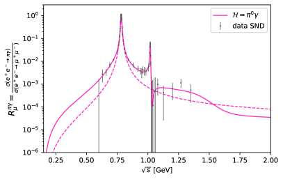
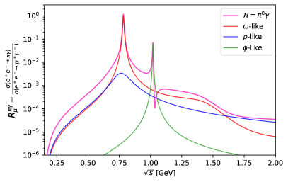
Figure 16: Normalized cross-section $R^{\mathcal{H}}_{\mu}$ for the $\mathcal{H}=\pi^{0}\gamma$ channel. In the left panel the solid (dashed) pink line indicates our (DarkCast) calculation, and the gray data points are from SND SND:2016drm . In the right panel we show our decomposition of the $\pi\gamma$ channel into $\rho$ (blue), $\omega$ (red) and $\phi$ (green) components.

For the case of the $KK$ channel, in the left panel of figure 17 we show the individual normalized cross sections for the neutral $K^{0}\bar{K}^{0}$ (light green) and charged $K^{+}K^{-}$(dark green) channels obtained using the fit from Plehn:2019jeo , along with the corresponding data points extracted from CLEO:2005tiu ; Achasov:2000am ; Achasov:2006bv ; Mane:1980ep ; CMD-3:2016nhy ; BaBar:2014uwz ; CMD-2:2008fsu ; BaBar:2013jqz ; BaBar:2015lgl ; Achasov:2016lbc . In solid (dashed) grey we show our (DarkCast) total $KK$ contribution, where for our calculation $KK=K^{0}\bar{K}^{0}+K^{+}K^{-}$, while in DarkCast $KK=2\;K^{+}K^{-}$. In the latter case, the reason for this definition is a consequence of the exclusive use of BaBar data from BaBar:2013jqz , which was a study that considered only the charged channel contribution. Here, we update the $KK$ channel description also by including recent data from several experiments.

In the right panel of figure 17, we present the decomposition of the charged $K^{+}K^{-}$ channel (dark green) into $\rho$ (blue), $\omega$ (red) and $\phi$ (green) components. It is important to emphasize that in DarkCast only the $\phi$-like component, that is responsible for the peak near $1$ GeV, is considered. However, the other features of the fit mainly come from the remaining vector meson contributions included in this study.

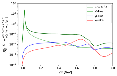
Figure 17: Normalized cross-section $R^{\mathcal{H}}_{\mu}$ for the $\mathcal{H}=KK$ channel. In the left panel the solid (dashed) gray line indicates our (DarkCast) total $KK$ calculation, while the dark (light) green line indicated our fit for the $K^{+}K^{-}$ ($K^{0}\bar{K}^{0}$) channel. The data points correspond to a compilation from several experiments CLEO:2005tiu ; Achasov:2000am ; Achasov:2006bv ; Mane:1980ep ; CMD-3:2016nhy ; BaBar:2014uwz ; CMD-2:2008fsu ; BaBar:2013jqz ; BaBar:2015lgl ; Achasov:2016lbc . In the right panel we show the decomposition of the charged $K^{+}K^{-}$ channel (dark green) into $\rho$ (blue), $\omega$ (red) and $\phi$ (green) components.

Finally, figure 18 shows the normalized cross section obtained using the fit from Plehn:2019jeo for the individually $KK\pi$ channels, together with the decomposition into $\phi$ (green) and $\rho$ (blue) contributions and the data points extracted from BaBar:2007ceh ; BaBar:2017nrz ; Achasov:2017vaq ; Bisello:1991kd ; Mane:1982si . The sum of these three channels results in the total $KK\pi$ channel considered in this work, in contrast to the $KK\pi$ used by DarkCast, which consists only of the isoscalar component and agrees with a different set of data BaBar:2007ceh . Hence, we not only consider a new vector component to the $KK\pi$ channel, but also used more recent data and described it correctly including separately the three components $K^{0}K^{0}\pi^{0}$, $K^{+}K^{-}\pi^{0}$ and $K^{\pm}K^{0}\pi^{\mp}$.

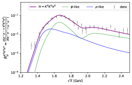
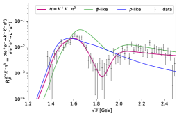
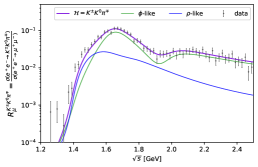
Figure 18: Normalized cross-section $R^{\mathcal{H}}_{\mu}$ for $\mathcal{H}=K^{0}K^{0}\pi^{0}$(left), $K^{+}K^{-}\pi^{0}$ (middle), $K^{\pm}K^{0}\pi^{\mp}$ (right). The purple lines correspond to the channel contribution, whereas the blue and green lines indicate the $\phi$ and $\rho$ decomposition, respectively. The data points from BaBar:2007ceh ; BaBar:2017nrz ; Achasov:2017vaq ; Bisello:1991kd ; Mane:1982si are shown in grey.

New channels:

Besides the additional channels described in Plehn:2019jeo that we include in this study, we add the description of four new channels, relevant in the higher energy region close to $2$ GeV. For the inclusion of these channels, first we need to identify all the possible intermediate structures. Then, if the data points are available, we can perform a fit using the python package IMinuit hans_dembinski_2021_5561211 . Below, we provide additional details concerning the method used for the computation of the fit for each of these new channels.

• $\mathcal{H}=\omega\pi\pi$

  In case of the $\omega\pi\pi$ final state, we distinguish between the charged mode $\omega\pi^{+}\pi^{-}$ and the neutral mode $\omega\pi^{0}\pi^{0}$, dominantly leading to the five pion final state combinations $2(\pi^{+}\pi^{-})\pi^{0}$ and $\pi^{+}\pi^{-}3\pi^{0}$, respectively. Although we have signs of possible intermediate substructures, such as $\omega f_{0}(980)\to\omega\pi^{+}\pi^{-}$ Aubert:2007ef and $b_{1}(1285)\pi\to\omega\pi\pi$ Achasov:1998sv , so far they have not been clearly seen in the data and hence, we will not consider them.

  Considering that G-parity only allows for $I=0$, we assume a point-like $\omega\to\omega\pi\pi$ interaction. The form factor is given by

  $$F_{\omega\pi\pi}=\sum_{V}\frac{a_{V}m_{V}^{2}e^{i\varphi_{V}}}{m_{V}^{2}-s-i\sqrt{s}\Gamma_{V}}\,,$$ (26)

  where the only vector meson relevant to describe this channel is $V=\omega^{\prime\prime}$, which corresponds to the $\omega(1650)$ meson. For the fit, we use data from Akhmetshin:2000wv ; Aubert:2007ef ; Lees:2018dnv . Table 4 lists the fit parameters obtained for this channel and figure 19 shows the curve of the fit with the hadronic data.

  Parameter	Fit Value	Parameter	Fit Value
  $m_{\omega^{\prime\prime}}$	$1.661\pm 0.007$ GeV	$\Gamma_{\omega^{\prime\prime}}$	$0.398\pm 0.021$ GeV
  $a_{\omega^{\prime\prime}}$	$2.73\pm 0.09$	$\varphi_{\omega^{\prime\prime}}$	$0$ (fixed)
  $\chi^{2}\mathrm{/n.d.f.}=1.67$

  Table 4: Values obtained by the fit for the $e^{+}e^{-}\to\omega\pi\pi$ current. The phase $\varphi_{\omega^{\prime\prime}}$ was fixed at $0$.

  

  

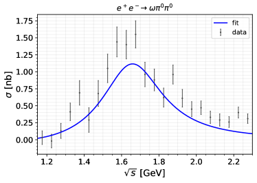
  Figure 19: Cross-section for the charged $\omega\pi^{+}\pi^{-}$ (left panel) and neutral $\omega\pi^{0}\pi^{0}$ (right panel) hadronic final states. The blue curve shows the best fit solution to the cross-section, obtained considering the fit values of table 4. The black points and error bars represent data from Akhmetshin:2000wv ; Aubert:2007ef ; Lees:2018dnv .

• $\mathcal{H}=K^{*}(892)K\pi$

  The $K^{*}(892)K\pi$ channel is the dominant contribution to $KK\pi\pi$ final states. Here, we consider the four most relevant intermediate substructures: $K^{*0}K^{\pm}\pi^{\mp}$, $K^{*\pm}K_{S}\pi^{\mp}$ and $K^{*\pm}K^{\mp}\pi^{0}$ decaying into $K_{S}K^{\pm}\pi^{\mp}\pi^{0}$, and $K^{*0}K^{\pm}\pi^{\mp}$ decaying into $K^{+}K^{-}\pi^{+}\pi^{-}$.

  In order to calculate the form factors we need to combine the isospin $I=0$ ($\phi$) and $I=1$ ($\rho$) contributions, corresponding to $A_{0}$ and $A_{1}$ amplitudes, respectively. The most general form factors assuming a point-like $V\to K^{*0}K^{\mp}\pi^{\pm}$ vertex structure can be written as

  $$K^{*0}K^{\pm}\pi^{\mp}\to K_{S}K^{\pm}\pi^{\mp}\pi^{0}:F_{(K^{*0}K^{\pm}\pi^{\mp})^{n}}=\frac{1}{\sqrt{18}}(A_{1}+A_{0})$$

  $$K^{*\pm}K_{S}\pi^{\mp}\to K_{S}K^{\pm}\pi^{\mp}\pi^{0}:F_{K^{*\pm}K_{S}\pi^{\mp}}=\frac{1}{\sqrt{18}}(A_{1}-A_{0})$$

  $$K^{*\mp}K^{\pm}\pi^{0}\to K_{S}K^{\pm}\pi^{\mp}\pi^{0}:F_{K^{*\pm}K^{\mp}\pi^{0}}=\frac{1}{\sqrt{18}}(A_{1}-A_{0})$$

  $$K^{*0}K^{\pm}\pi^{\mp}\to K^{+}K^{-}\pi^{+}\pi^{-}:F_{(K^{*0}K^{\pm}\pi^{\mp})^{c}}=\sqrt{\frac{2}{9}}(A_{1}+A_{0})~{},$$

  where we denote the form factor of the $K^{*0}K^{\pm}\pi^{\mp}$ state decaying into the neutral (charged) $K_{S}K^{\pm}\pi^{\mp}\pi^{0}$ ($K^{+}K^{-}\pi^{+}\pi^{-}$) with a n (c) superscript and the isospin amplitudes are given by

  $$A_{0} =\sum_{\phi}\frac{a_{\phi}e^{i\varphi_{\phi}}m_{\phi}^{2}}{m_{\phi}^{2}-s-im_{\phi}\Gamma_{\phi}}~{},$$

  $$A_{1} =\sum_{\rho}\frac{a_{\rho}e^{i\varphi_{\rho}}m_{\rho}^{2}}{m_{\rho}^{2}-s-im_{\rho}\Gamma_{\rho}}~{}.$$ (27)

  The data used to perform the fit was taken from BaBar BaBar:2011btv ; BaBar:2017pkz , and the vector meson resonances found by the fit to describe this channel were $V=\phi^{\prime},\rho^{\prime\prime}$. Table 5 summarizes the obtained fit parameters and figure 20 shows the curve of the best fit solution for each of these four $KK\pi\pi$ states.

  $K_{S}K^{\pm}\pi^{\mp}\pi^{0}$		$K^{+}K^{-}\pi^{+}\pi^{-}$
  Parameter	Fit Value	Parameter	Fit Value
  $m_{\phi^{\prime}}$	$1.7$ GeV (fixed)	$m_{\phi^{\prime}}$	$1.65$ GeV (fixed)
  $a_{\phi^{\prime}}$	$2.49\pm 0.6$	$a_{\phi^{\prime}}$	$4.52\pm 0.5$
  $\Gamma_{\phi^{\prime}}$	$0.3$ GeV (fixed)	$\Gamma_{\phi^{\prime}}$	$0.103\pm 0.009$
  $\varphi_{\phi^{\prime}}$	$1.02\pm 0.09$	$\varphi_{\phi^{\prime}}$	$\pi$ (fixed)
  $m_{\rho^{\prime\prime}}$	$1.898\pm 0.012$ GeV	$m_{\rho^{\prime\prime}}$	$1.842\pm 0.011$ GeV
  $a_{\rho^{\prime\prime}}$	$13.5\pm 0.5$	$a_{\rho^{\prime\prime}}$	$15.7\pm 1.0$
  $\Gamma_{\rho^{\prime\prime}}$	$0.504\pm 0.021$ GeV	$\Gamma_{\rho^{\prime\prime}}$	$0.403\pm 0.016$ GeV
  $\varphi_{\rho^{\prime\prime}}$	$0$ (fixed)	$\varphi_{\rho^{\prime\prime}}$	$0.000\pm 0.006$
  $\chi^{2}\mathrm{/n.d.f.}=2.68$		$\chi^{2}\mathrm{/n.d.f.}=1.59$

  Table 5: Values obtained by the fit to the $e^{+}e^{-}\to K^{*}K\pi\to K_{S}K^{\pm}\pi^{\mp}\pi^{0}$ current (left) and to the $e^{+}e^{-}\to K^{*}K\pi\to K^{+}K^{-}\pi^{+}\pi^{-}$ current (right).

  

  

  

  

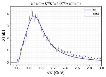
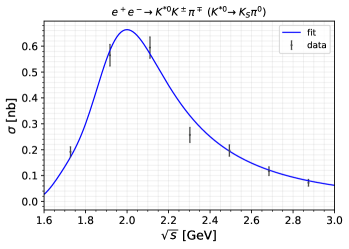
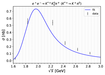
  Figure 20: Cross-section for the charged $K^{*0}K^{\pm}\pi^{\mp}$ (upper left panel), neutral $K^{*0}K^{\pm}\pi^{\mp}$ (upper right panel), $K^{*\pm}K_{S}\pi^{\mp}$ (lower left panel) and $K^{*\mp}K^{\pm}\pi^{0}$ (lower right panel) hadronic final states. The blue curve shows the best fit solution to the cross-section, obtained considering the fit values of table 5. The black points and error bars represent data from BaBar:2011btv ; BaBar:2017pkz .

• $\mathcal{H}=\phi\pi\pi$

  The $\phi\pi\pi$ channel can be decomposed into a charged ($\phi\pi^{+}\pi^{-}$) and a neutral ($\phi\pi^{0}\pi^{0}$) component. Due to the decay of the $\phi$ meson into two kaons, $\phi(1020)\to K^{+}K^{-}$, the charged (neutral) component represents a small contribution to the $K^{+}K^{-}\pi^{+}\pi^{-}$ ($K^{+}K^{-}\pi^{0}\pi^{0}$) state.

  In the energy region relevant in this study, we can describe both $\phi\pi\pi$ states by the first two excited $\phi$ resonances $\phi^{\prime}$ and $\phi^{\prime\prime}$. The form factor is given by

  $$F_{\phi\pi\pi}=\sum_{V}\frac{a_{V}m_{V}^{2}e^{i\varphi_{V}}}{m_{V}^{2}-s-i\sqrt{s}\Gamma_{V}}~{},$$ (28)

  with $V=\phi^{\prime},\phi^{\prime\prime}$. The data considered for the fit was taken from BaBar:2011btv ; Belle:2008kuo and the values for the parameters obtained in the fit, for both the neutral and charged states, can be found in table 6. Figure 21 shows the curve of the best fit together with the data points.

  Parameter	Fit Value	Parameter	Fit Value
  $m_{\phi^{\prime}}$	$1.680\pm 0.012$ GeV	$m_{\phi^{\prime\prime}}$	$2.162\pm 0.015$ GeV
  $a_{\phi^{\prime}}$	$1.44\pm 0.16$	$a_{\phi^{\prime\prime}}$	$0.69\pm 0.11$
  $\Gamma_{\phi^{\prime}}$	$0.226\pm 0.021$ GeV	$\Gamma_{\phi^{\prime\prime}}$	$0.209\pm 0.025$ GeV
  $\varphi_{\phi^{\prime}}$	$2.6\pm 0.4$	$\varphi_{\phi^{\prime\prime}}$	$0$ (fixed)
  $\chi^{2}\mathrm{/n.d.f.}=0.55$

  Table 6: Values obtained by the fit for the $e^{+}e^{-}\to\phi\pi\pi$ current.

  

  

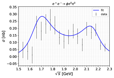
  Figure 21: Cross-section for the charged $\phi\pi^{+}\pi^{-}$ (left panel) and neutral $\phi\pi^{0}\pi^{0}$ (right panel) hadronic final states. The blue curve shows the best fit solution to the cross-section, obtained considering the fit values of table 6. The black points and error bars represent data from BaBar:2011btv ; Belle:2008kuo .

• $\mathcal{H}=6\pi$

  For the case of the $6\pi$ channel, we considered a charged state $3(\pi^{+}\pi^{-})$ and a neutral state $2(\pi^{+}\pi^{-}\pi^{0})$. In this particular case, we cannot describe these channels by identifying the Breit-Wigner resonances. The available data does not indicate any clear intermediate structures, suggesting that the description of the $6\pi$ channel can only proceed via the inclusion of the decays of many different vector states. Following BaBar:2006vzy ; Achasov:1996gw , we fitted the $6\pi$ cross-section according to the parametrization given by

  $$\sigma_{6\pi}=\frac{4\pi\alpha^{2}}{s^{3/2}}\left(\frac{a_{V}m_{V}^{2}e^{i\varphi_{V}}}{s-m_{V}^{2}+i\sqrt{s}\Gamma_{V}}+A_{\rm cont}\right)^{2}\,,$$ (29)

  where

  $$A_{\rm cont}=c_{0}+c_{1}\frac{e^{-b/(\sqrt{s}-m_{0})}}{(\sqrt{s}-m_{0})^{2-a}}$$ (30)

  is a Jacob-Slansky amplitude PhysRevD.5.1847 that accounts for the mixture of several broad resonances, and the parameters $c_{0},c_{1},a,b,m_{0}$ are free variables. Due to G-parity symmetry arguments we can identify $V$ with the higher excitation of the $\rho$ vector meson, namely $V=\rho^{\prime\prime\prime}$. Table 7 shows the values of the free parameters obtained by our fit using the parameterization described above and the data from BaBar:2006vzy . Figure 22 shows the best fit solution to the cross-section for both the charged and neutral $6\pi$ states.

  $3(\pi^{+}\pi^{-})$		$2(\pi^{+}\pi^{-}\pi^{0})$
  Parameter	Fit Value	Parameter	Fit Value
  $m_{\rho^{\prime\prime\prime}}$	$1.88$ GeV (fixed)	$m_{\rho^{\prime\prime\prime}}$	$1.86$ GeV (fixed)
  $a_{\rho^{\prime\prime\prime}}$	$0.0037\pm 0.0005\,\mathrm{GeV}^{1/2}$	$a_{\rho^{\prime\prime\prime}}$	$-0.0072\pm 0.0009\,\mathrm{GeV}^{1/2}$
  $\Gamma_{\rho^{\prime\prime\prime}}$	$0.13$ GeV (fixed)	$\Gamma_{\rho^{\prime\prime\prime}}$	$0.16$ GeV (fixed)
  $\varphi_{\rho^{\prime\prime\prime}}$	$0.367$ (fixed)	$\varphi_{\rho^{\prime\prime\prime}}$	$-0.052$ (fixed)
  $c_{0}$	$0.0153\pm 0.0029\,\mathrm{GeV}^{1/2}$	$c_{0}$	$-0.028\pm 0.009\,\mathrm{GeV}^{1/2}$
  $c_{1}$	$-1.082\pm 0.017\,\mathrm{GeV}^{(5/2-a)}$	$c_{1}$	$2.4\pm 0.7\,\mathrm{GeV}^{(5/2-a)}$
  $b$	$1.40\pm 0.01$ GeV	$b$	$1.54\pm 0.32$ GeV
  $a$	$0.89\pm 0.04$	$a$	$0.85\pm 0.23$
  $m_{0}$	$1.262\pm 0.012$ GeV	$m_{0}$	$1.20\pm 0.04$ GeV
  $\chi^{2}\mathrm{/n.d.f.}=0.6$		$\chi^{2}\mathrm{/n.d.f.}=0.7$

  Table 7: Fit values for the $e^{+}e^{-}\to 3(\pi^{+}\pi^{-})$ current (left) and for the $e^{+}e^{-}\to 2(\pi^{+}\pi^{-})\pi^{0}\pi^{0}$ current (right). The values of $m_{\rho^{\prime\prime\prime}}$, $\Gamma_{\rho^{\prime\prime\prime}}$ and $\varphi_{\rho^{\prime\prime\prime}}$ were taken from BaBar:2006vzy .

  

  

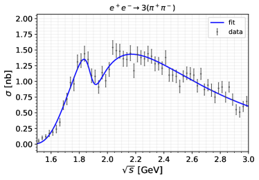
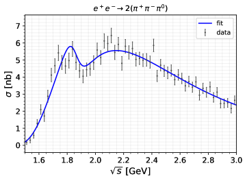
  Figure 22: Cross-section for the charged $3(\pi^{+}\pi^{-})$ (left panel) and neutral $2(\pi^{+}\pi^{-}\pi^{0})$ (right panel) hadronic final states. The blue curve shows the best fit solution to the cross-section, obtained considering the parameterization described in eq. (29) and (30) and the fit values of table 7. The black points and error bars represent data from BaBar:2006vzy .

Appendix C Hadronic Decay Package

We provide the results of calculating hadronic decays and related quantities in the python package DeLiVeR. Here, we briefly describe the structure of the code. Further instructions and more practical advices are provided in the package as jupyter notebooks.

Model definition:

As a first step, the user must define the model by specifying i) the $Q$-charges $q_{Q}^{f}$ and the $U(1)_{Q}$ coupling constant $g_{Q}$, ii) if the mediator is coupling to DM, and if yes, in which way. Possible candidates are a Majorana Batell:2021blf ; Batell:2021aja , or Dirac fermion MiniBooNEDM:2018cxm , a complex scalar particle MiniBooNE:2017nqe ; MiniBooNEDM:2018cxm ; DeRomeri:2019kic ; Batell:2021blf ; Batell:2021aja , or inelastic pseudo-Dirac DM Berlin:2018bsc ; Batell:2021ooj . For all DM types, the DM mass $m_{\chi}$ is set in relation to the mediator mass via $R_{\chi}=m_{\chi}/m_{Z_{Q}}$ as it is common practice in the literature and the mediator-DM coupling strength can be specified as well. In case of inelastic DM, the mass splitting between the DM states has to be defined as well. As we focus on hadronic decays of vector particles, we refrain from including an invisible DM decay of vector mediators in the results presented above and leave this study for future work.

Width calculation:

In order to calculate the decay widths of the $Z_{Q}$ mediator in the specified model, the width class is initiated by using the model as an input. As described in section IV, some channels $\mathcal{H}$ are sums of several final state configurations. For example $\mathcal{H}=4\pi$ consists of $2\pi^{+}2\pi^{-}$ and $\pi^{+}\pi^{-}2\pi^{0}$. Additionally to the summed contributions, the user can calculate single sub-contributions within the width class. Besides all contributions, the total width and lifetime of the particle is calculated without further ado.

Branching ratios:

All calculated widths can then be used to calculate the branching ratios for all channels, as well as to determine the visible, invisible and hadronic width of the vector mediator.

R-ratio:

In the style of the typical way of calculating the dark photon decay width as in eq. (10), the user can calculate the $R_{\mu}^{\mathcal{H}}$ values for arbitrary vector mediator models. Multiplied by the decay width $\Gamma_{Z_{Q}\to\mu^{+}\mu^{-}}$ this yields the partial decay width $\Gamma_{Z_{Q}\to\mathcal{H}}$. This method is most useful for the dark photon, but can in principle also be used by other models. In this case the $R_{\mu}^{\mathcal{H}}$ should be less seen as a ratio of $\sigma(e^{+}e^{-}\to\mathcal{H})/\sigma(e^{+}e^{-}\to\mu^{+}\mu^{-})$ but more simply as $\Gamma_{Z_{Q}\to\mathcal{H}}/\Gamma_{Z_{Q}\to\mu^{+}\mu^{-}}$.

References

- (1) M. Pospelov, A. Ritz, and M. B. Voloshin, “Secluded WIMP Dark Matter,” Phys. Lett. B 662 (2008) 53–61, arXiv:0711.4866 [hep-ph].
- (2) A. Kamada, K. Kaneta, K. Yanagi, and H.-B. Yu, “Self-interacting dark matter and muon in a gauged U model,” JHEP 06 (2018) 117, arXiv:1805.00651 [hep-ph].
- (3) T. Plehn, P. Reimitz, and P. Richardson, “Hadronic Footprint of GeV-Mass Dark Matter,” SciPost Phys. 8 (2020) 092, arXiv:1911.11147 [hep-ph].
- (4) D. Borah, M. Dutta, S. Mahapatra, and N. Sahu, “Muon (g2) and XENON1T excess with boosted dark matter in LL model,” Phys. Lett. B 820 (2021) 136577, arXiv:2104.05656 [hep-ph].
- (5) S. Singirala, S. Sahoo, and R. Mohanta, “Light dark matter, rare decays with missing energy in model with a scalar leptoquark,” arXiv:2106.03735 [hep-ph].
- (6) I. Holst, D. Hooper, and G. Krnjaic, “The Simplest and Most Predictive Model of Muon and Thermal Dark Matter,” arXiv:2107.09067 [hep-ph].
- (7) B. Batell, J. L. Feng, M. Fieg, A. Ismail, F. Kling, R. M. Abraham, and S. Trojanowski, “Hadrophilic Dark Sectors at the Forward Physics Facility,” arXiv:2111.10343 [hep-ph].
- (8) S. Baek, N. G. Deshpande, X. G. He, and P. Ko, “Muon anomalous g-2 and gauged L(muon) - L(tau) models,” Phys. Rev. D 64 (2001) 055006, arXiv:hep-ph/0104141.
- (9) M. Pospelov, “Secluded U(1) below the weak scale,” Phys. Rev. D 80 (2009) 095002, arXiv:0811.1030 [hep-ph].
- (10) E. Bertuzzo, S. Jana, P. A. N. Machado, and R. Zukanovich Funchal, “Dark Neutrino Portal to Explain MiniBooNE excess,” Phys. Rev. Lett. 121 no. 24, (2018) 241801, arXiv:1807.09877 [hep-ph].
- (11) P. Ballett, S. Pascoli, and M. Ross-Lonergan, “U(1)’ mediated decays of heavy sterile neutrinos in MiniBooNE,” Phys. Rev. D 99 (2019) 071701, arXiv:1808.02915 [hep-ph].
- (12) M. Escudero, D. Hooper, G. Krnjaic, and M. Pierre, “Cosmology with A Very Light Lμ-Lτ Gauge Boson,” JHEP 03 (2019) 071, arXiv:1901.02010 [hep-ph].
- (13) P. Ilten, Y. Soreq, M. Williams, and W. Xue, “Serendipity in dark photon searches,” JHEP 06 (2018) 004, arXiv:1801.04847 [hep-ph].
- (14) M. Bauer, P. Foldenauer, and J. Jaeckel, “Hunting All the Hidden Photons,” JHEP 07 (2018) 094, arXiv:1803.05466 [hep-ph].
- (15) H. Dembinski, P. Ongmongkolkul, C. Deil, D. M. Hurtado, H. Schreiner, M. Feickert, Andrew, C. Burr, J. Watson, F. Rost, A. Pearce, L. Geiger, B. M. Wiedemann, C. Gohlke, Gonzalo, J. Drotleff, J. Eschle, L. Neste, M. E. Gorelli, M. Baak, O. Zapata, and odidev, “scikit-hep/iminuit: v2.8.4,” Oct., 2021. https://doi.org/10.5281/zenodo.5561211.
- (16) G. Rodrigo, H. Czyz, J. H. Kuhn, and M. Szopa, “Radiative return at NLO and the measurement of the hadronic cross-section in electron positron annihilation,” Eur. Phys. J. C 24 (2002) 71–82, arXiv:hep-ph/0112184.
- (17) H. Czyż, P. Kisza, and S. Tracz, “Modeling interactions of photons with pseudoscalar and vector mesons,” Phys. Rev. D 97 no. 1, (2018) 016006, arXiv:1711.00820 [hep-ph].
- (18) B. Holdom, “Two U(1)’s and Epsilon Charge Shifts,” Phys. Lett. B 166 (1986) 196–198.
- (19) T. Araki, J. Heeck, and J. Kubo, “Vanishing Minors in the Neutrino Mass Matrix from Abelian Gauge Symmetries,” JHEP 07 (2012) 083, arXiv:1203.4951 [hep-ph].
- (20) S. H. Seo and Y. D. Kim, “Dark Photon Search at Yemilab, Korea,” JHEP 04 (2021) 135, arXiv:2009.11155 [hep-ph].
- (21) S. Scherer, “Introduction to chiral perturbation theory,” Adv. Nucl. Phys. 27 (2003) 277, arXiv:hep-ph/0210398.
- (22) J. J. Sakurai, “Theory of strong interactions,” Annals Phys. 11 (1960) 1–48.
- (23) N. M. Kroll, T. D. Lee, and B. Zumino, “Neutral Vector Mesons and the Hadronic Electromagnetic Current,” Phys. Rev. 157 (1967) 1376–1399.
- (24) T. D. Lee and B. Zumino, “Field Current Identities and Algebra of Fields,” Phys. Rev. 163 (1967) 1667–1681.
- (25) S. Tulin, “New weakly-coupled forces hidden in low-energy QCD,” Phys. Rev. D 89 no. 11, (2014) 114008, arXiv:1404.4370 [hep-ph].
- (26) H. B. O’Connell, B. C. Pearce, A. W. Thomas, and A. G. Williams, “ mixing, vector meson dominance and the pion form-factor,” Prog. Part. Nucl. Phys. 39 (1997) 201–252, arXiv:hep-ph/9501251.
- (27) M. Bando, T. Kugo, S. Uehara, K. Yamawaki, and T. Yanagida, “Is rho Meson a Dynamical Gauge Boson of Hidden Local Symmetry?,” Phys. Rev. Lett. 54 (1985) 1215.
- (28) T. Fujiwara, T. Kugo, H. Terao, S. Uehara, and K. Yamawaki, “Nonabelian Anomaly and Vector Mesons as Dynamical Gauge Bosons of Hidden Local Symmetries,” Prog. Theor. Phys. 73 (1985) 926.
- (29) G. Kramer, W. F. Palmer, and S. S. Pinsky, “Testing Chiral Anomalies With Hadronic Currents,” Phys. Rev. D 30 (1984) 89.
- (30) M. Bando, T. Kugo, and K. Yamawaki, “On the Vector Mesons as Dynamical Gauge Bosons of Hidden Local Symmetries,” Nucl. Phys. B 259 (1985) 493.
- (31) M. Bando, T. Kugo, and K. Yamawaki, “Nonlinear Realization and Hidden Local Symmetries,” Phys. Rept. 164 (1988) 217–314.
- (32) J. Wess and B. Zumino, “Consequences of anomalous Ward identities,” Phys. Lett. B 37 (1971) 95–97.
- (33) E. Witten, “Global Aspects of Current Algebra,” Nucl. Phys. B 223 (1983) 422–432.
- (34) Particle Data Group Collaboration, P. A. Zyla et al., “Review of Particle Physics,” PTEP 2020 no. 8, (2020) 083C01.
- (35) BaBar Collaboration, B. Aubert et al., “The e+ e- 2(pi+ pi-) pi0, 2(pi+ pi-) eta, K+ K- pi+ pi- pi0 and K+ K- pi+ pi- eta Cross Sections Measured with Initial-State Radiation,” Phys. Rev. D 76 (2007) 092005, arXiv:0708.2461 [hep-ex]. [Erratum: Phys.Rev.D 77, 119902 (2008)].
- (36) BaBar Collaboration, J. P. Lees et al., “Study of the reactions and at center-of-mass energies from threshold to 4.35 GeV using initial-state radiation,” Phys. Rev. D 98 no. 11, (2018) 112015, arXiv:1810.11962 [hep-ex].
- (37) BaBar Collaboration, B. Aubert et al., “Measurements of , and cross- sections using initial state radiation events,” Phys. Rev. D 77 (2008) 092002, arXiv:0710.4451 [hep-ex].
- (38) SND Collaboration, M. N. Achasov et al., “Study of the reaction with the SND detector at the VEPP-2M collider,” Phys. Rev. D 93 no. 9, (2016) 092001, arXiv:1601.08061 [hep-ex].
- (39) KLOE Collaboration, F. Ambrosino et al., “Measurement of and the dipion contribution to the muon anomaly with the KLOE detector,” Phys. Lett. B 670 (2009) 285–291, arXiv:0809.3950 [hep-ex].
- (40) BaBar Collaboration, B. Aubert et al., “Precise measurement of the e+ e- pi+ pi- (gamma) cross section with the Initial State Radiation method at BABAR,” Phys. Rev. Lett. 103 (2009) 231801, arXiv:0908.3589 [hep-ex].
- (41) BaBar Collaboration, J. P. Lees et al., “Precise Measurement of the Cross Section with the Initial-State Radiation Method at BABAR,” Phys. Rev. D 86 (2012) 032013, arXiv:1205.2228 [hep-ex].
- (42) H. Czyz, A. Grzelinska, and J. H. Kuhn, “Narrow resonances studies with the radiative return method,” Phys. Rev. D 81 (2010) 094014, arXiv:1002.0279 [hep-ph].
- (43) BaBar Collaboration, B. Aubert et al., “Study of process using initial state radiation with BaBar,” Phys. Rev. D 70 (2004) 072004, arXiv:hep-ex/0408078.
- (44) H. Czyz, A. Grzelinska, J. H. Kuhn, and G. Rodrigo, “Electron-positron annihilation into three pions and the radiative return,” Eur. Phys. J. C 47 (2006) 617–624, arXiv:hep-ph/0512180.
- (45) BaBar Collaboration, J. P. Lees et al., “Initial-State Radiation Measurement of the Cross Section,” Phys. Rev. D 85 (2012) 112009, arXiv:1201.5677 [hep-ex].
- (46) BaBar Collaboration, J. P. Lees et al., “Measurement of the cross section using initial-state radiation at BABAR,” Phys. Rev. D 96 no. 9, (2017) 092009, arXiv:1709.01171 [hep-ex].
- (47) H. Czyz, J. H. Kuhn, and A. Wapienik, “Four-pion production in tau decays and e+e- annihilation: An Update,” Phys. Rev. D 77 (2008) 114005, arXiv:0804.0359 [hep-ph].
- (48) CLEO Collaboration, T. K. Pedlar et al., “Precision measurements of the timelike electromagnetic form-factors of pion, kaon, and proton,” Phys. Rev. Lett. 95 (2005) 261803, arXiv:hep-ex/0510005.
- (49) M. N. Achasov et al., “Measurements of the parameters of the resonance through studies of the processes , , and ,” Phys. Rev. D 63 (2001) 072002, arXiv:hep-ex/0009036.
- (50) M. N. Achasov et al., “Experimental study of the reaction e+ e- K(S)K(L) in the energy range s**(1/2) = 1.04-GeV divided by 1.38-GeV,” J. Exp. Theor. Phys. 103 no. 5, (2006) 720–727, arXiv:hep-ex/0606057.
- (51) F. Mane, D. Bisello, J. C. Bizot, J. Buon, A. Cordier, and B. Delcourt, “Study of the Reaction in the Total Energy Range 1.4-GeV to 2.18-GeV and Interpretation of the and Form-factors,” Phys. Lett. B 99 (1981) 261–264.
- (52) CMD-3 Collaboration, E. A. Kozyrev et al., “Study of the process in the center-of-mass energy range 1004–1060 MeV with the CMD-3 detector at the VEPP-2000 collider,” Phys. Lett. B 760 (2016) 314–319, arXiv:1604.02981 [hep-ex].
- (53) BaBar Collaboration, J. P. Lees et al., “Cross sections for the reactions , , , and from events with initial-state radiation,” Phys. Rev. D 89 no. 9, (2014) 092002, arXiv:1403.7593 [hep-ex].
- (54) CMD-2 Collaboration, R. R. Akhmetshin et al., “Measurement of cross section with the CMD-2 detector at VEPP-2M Collider,” Phys. Lett. B 669 (2008) 217–222, arXiv:0804.0178 [hep-ex].
- (55) BaBar Collaboration, J. P. Lees et al., “Precision measurement of the cross section with the initial-state radiation method at BABAR,” Phys. Rev. D 88 no. 3, (2013) 032013, arXiv:1306.3600 [hep-ex].
- (56) BaBar Collaboration, J. P. Lees et al., “Study of the reaction in the energy range from 2.6 to 8.0 GeV,” Phys. Rev. D 92 no. 7, (2015) 072008, arXiv:1507.04638 [hep-ex].
- (57) M. N. Achasov et al., “Measurement of the cross section in the energy range GeV” Phys. Rev. D 94 no. 11, (2016) 112006, arXiv:1608.08757 [hep-ex].
- (58) BaBar Collaboration, J. P. Lees et al., “Cross sections for the reactions , , and from events with initial-state radiation,” Phys. Rev. D 95 no. 5, (2017) 052001, arXiv:1701.08297 [hep-ex].
- (59) M. N. Achasov et al., “Measurement of the cross section in the energy range GeV” Phys. Rev. D 97 no. 3, (2018) 032011, arXiv:1711.07143 [hep-ex].
- (60) D. Bisello et al., “Observation of an isoscalar vector meson at approximately = 1650-MeV/c**2 in the e+ e- K anti-K pi reaction,” Z. Phys. C 52 (1991) 227–230.
- (61) F. Mane, D. Bisello, J. C. Bizot, J. Buon, A. Cordier, and B. Delcourt, “Study of in the 1.4-GeV to 2.18-GeV Energy Range: A New Observation of an Isoscalar Vector Meson (1.65-GeV),” Phys. Lett. B 112 (1982) 178–182.
- (62) M. N. Achasov et al., “Study of the e+ e- eta gamma process with SND detector at the VEPP-2M e+ e- collider,” Phys. Rev. D 74 (2006) 014016, arXiv:hep-ex/0605109.
- (63) M. N. Achasov et al., “Measurement of the e+ e- cross section with the SND detector at the VEPP-2000 collider,” Phys. Rev. D 97 no. 1, (2018) 012008, arXiv:1711.08862 [hep-ex].
- (64) BaBar Collaboration, J. P. Lees et al., “Study of the process using initial state radiation,” Phys. Rev. D 97 (2018) 052007, arXiv:1801.02960 [hep-ex].
- (65) H. Czyż, M. Gunia, and J. H. Kühn, “Simulation of electron-positron annihilation into hadrons with the event generator PHOKHARA,” JHEP 08 (2013) 110, arXiv:1306.1985 [hep-ph].
- (66) M. N. Achasov et al., “Updated measurement of the cross section with the SND detector,” Phys. Rev. D 94 no. 11, (2016) 112001, arXiv:1610.00235 [hep-ex].
- (67) CMD-2 Collaboration, R. R. Akhmetshin et al., “Study of the process e+ e- pi+ pi- pi+ pi- pi0 with CMD-2 detector,” Phys. Lett. B 489 (2000) 125–130, arXiv:hep-ex/0009013.
- (68) BaBar Collaboration, J. P. Lees et al., “Cross sections for the reactions , , and from events with initial-state radiation,” Phys. Rev. D 95 no. 5, (2017) 052001, arXiv:1701.08297 [hep-ex].
- (69) M. N. Achasov et al., “Measurement of the cross section below GeV,” Phys. Rev. D 94 no. 9, (2016) 092002, arXiv:1607.00371 [hep-ex].
- (70) M. N. Achasov et al., “Measurement of the e+e- Cross Section by Means of the SND Detector,” Phys. Atom. Nucl. 81 no. 2, (2018) 205–213.
- (71) BaBar Collaboration, J. P. Lees et al., “Study of via initial-state radiation at BABAR,” Phys. Rev. D87 no. 9, (2013) 092005, arXiv:1302.0055 [hep-ex].
- (72) BESIII Collaboration, M. Ablikim et al., “Measurement of the proton form factor by studying ,” Phys. Rev. D91 no. 11, (2015) 112004, arXiv:1504.02680 [hep-ex].
- (73) CLEO Collaboration, T. K. Pedlar et al., “Precision measurements of the timelike electromagnetic form-factors of pion, kaon, and proton,” Phys. Rev. Lett. 95 (2005) 261803, arXiv:hep-ex/0510005 [hep-ex].
- (74) B. Delcourt et al., “Study of the Reaction in the Total Energy Range 1925-MeV - 2180-MeV,” Phys. Lett. 86B (1979) 395–398.
- (75) M. Castellano, G. Di Giugno, J. W. Humphrey, E. Sassi Palmieri, G. Troise, U. Troya, and S. Vitale, “The reaction at a total energy of 2.1 gev,” Nuovo Cim. A14 (1973) 1–20.
- (76) A. Antonelli et al., “The first measurement of the neutron electromagnetic form-factors in the timelike region,” Nucl. Phys. B517 (1998) 3–35.
- (77) E760 Collaboration, T. A. Armstrong et al., “Measurement of the proton electromagnetic form-factors in the timelike region at ,” Phys. Rev. Lett. 70 (1993) 1212–1215.
- (78) E835 Collaboration, M. Ambrogiani et al., “Measurements of the magnetic form-factor of the proton in the timelike region at large momentum transfer,” Phys. Rev. D60 (1999) 032002.
- (79) M. Andreotti et al., “Measurements of the magnetic form-factor of the proton for timelike momentum transfers,” Phys. Lett. B559 (2003) 20–25.
- (80) V. Punjabi et al., “Proton elastic form-factor ratios to by polarization transfer,” Phys. Rev. C71 (2005) 055202, arXiv:nucl-ex/0501018 [nucl-ex]. [Erratum: Phys. Rev.C71,069902(2005)].
- (81) A. J. R. Puckett et al., “Final Analysis of Proton Form Factor Ratio Data at , 4.8 and 5.6 GeV2,” Phys. Rev. C85 (2012) 045203, arXiv:1102.5737 [nucl-ex].
- (82) O. Gayou et al., “Measurements of the elastic electromagnetic form-factor ratio mu(p) G(Ep) / G(Mp) via polarization transfer,” Phys. Rev. C64 (2001) 038202.
- (83) A. J. R. Puckett et al., “Recoil Polarization Measurements of the Proton Electromagnetic Form Factor Ratio to ,” Phys. Rev. Lett. 104 (2010) 242301, arXiv:1005.3419 [nucl-ex].
- (84) A. J. R. Puckett et al., “Polarization Transfer Observables in Elastic Electron Proton Scattering at 2.5, 5.2, 6.8, and 8.5 GeV2,” Phys. Rev. C96 no. 5, (2017) 055203, arXiv:1707.08587 [nucl-ex]. [erratum: Phys. Rev.C98,no.1,019907(2018)].
- (85) A1 Collaboration, T. Pospischil et al., “Measurement of G(E(p))/G(M(p)) via polarization transfer at ,” Eur. Phys. J. A12 (2001) 125–127.
- (86) Jefferson Laboratory E93-038 Collaboration, B. Plaster et al., “Measurements of the neutron electric to magnetic form-factor ratio G(En) / G(Mn) via the H-2(polarized-e, e-prime,polarized-n)H-1 reaction to ,” Phys. Rev. C73 (2006) 025205, arXiv:nucl-ex/0511025 [nucl-ex].
- (87) BLAST Collaboration, E. Geis et al., “The Charge Form Factor of the Neutron at Low Momentum Transfer from the H-2-polarized (e-polarized, e-prime n) p Reaction,” Phys. Rev. Lett. 101 (2008) 042501, arXiv:0803.3827 [nucl-ex].
- (88) L. Andivahis et al., “Measurements of the electric and magnetic form-factors of the proton from to ,” Phys. Rev. D50 (1994) 5491–5517.
- (89) H. Czyż, J. H. Kühn, and S. Tracz, “Nucleon form factors and final state radiative corrections to ,” Phys. Rev. D 90 no. 11, (2014) 114021, arXiv:1407.7995 [hep-ph].
- (90) BaBar Collaboration, J. P. Lees et al., “Cross Sections for the Reactions e+e- K+ K- pi+pi-, K+ K- pi0pi0, and K+ K- K+ K- Measured Using Initial-State Radiation Events,” Phys. Rev. D 86 (2012) 012008, arXiv:1103.3001 [hep-ex].
- (91) Belle Collaboration, C. P. Shen et al., “Observation of the phi(1680) and the Y(2175) in e+e- phi pi+ pi-,” Phys. Rev. D 80 (2009) 031101, arXiv:0808.0006 [hep-ex].
- (92) BaBar Collaboration, J. P. Lees et al., “Measurement of the and cross sections using initial-state radiation,” Phys. Rev. D 95 no. 9, (2017) 092005, arXiv:1704.05009 [hep-ex].
- (93) BaBar Collaboration, B. Aubert et al., “The and cross sections at center-of-mass energies from production threshold to 4.5-GeV measured with initial-state radiation,” Phys. Rev. D 73 (2006) 052003, arXiv:hep-ex/0602006.
- (94) F. Kling and S. Trojanowski, “Forward experiment sensitivity estimator for the LHC and future hadron colliders,” Phys. Rev. D 104 no. 3, (2021) 035012, arXiv:2105.07077 [hep-ph].
- (95) APEX Collaboration, S. Abrahamyan et al., “Search for a New Gauge Boson in Electron-Nucleus Fixed-Target Scattering by the APEX Experiment,” Phys. Rev. Lett. 107 (2011) 191804, arXiv:1108.2750 [hep-ex].
- (96) A1 Collaboration, H. Merkel et al., “Search for Light Gauge Bosons of the Dark Sector at the Mainz Microtron,” Phys. Rev. Lett. 106 (2011) 251802, arXiv:1101.4091 [nucl-ex].
- (97) H. Merkel et al., “Search at the Mainz Microtron for Light Massive Gauge Bosons Relevant for the Muon g-2 Anomaly,” Phys. Rev. Lett. 112 no. 22, (2014) 221802, arXiv:1404.5502 [hep-ex].
- (98) NA64 Collaboration, D. Banerjee et al., “Search for invisible decays of sub-GeV dark photons in missing-energy events at the CERN SPS,” Phys. Rev. Lett. 118 no. 1, (2017) 011802, arXiv:1610.02988 [hep-ex].
- (99) NA64 Collaboration, D. Banerjee et al., “Search for vector mediator of Dark Matter production in invisible decay mode,” Phys. Rev. D 97 no. 7, (2018) 072002, arXiv:1710.00971 [hep-ex].
- (100) D. Banerjee et al., “Dark matter search in missing energy events with NA64,” Phys. Rev. Lett. 123 no. 12, (2019) 121801, arXiv:1906.00176 [hep-ex].
- (101) LSND Collaboration, C. Athanassopoulos et al., “Evidence for muon-neutrino electron-neutrino oscillations from pion decay in flight neutrinos,” Phys. Rev. C 58 (1998) 2489–2511, arXiv:nucl-ex/9706006.
- (102) G. Bernardi et al., “Search for Neutrino Decay,” Phys. Lett. B 166 (1986) 479–483.
- (103) J. Blumlein et al., “Limits on the mass of light (pseudo)scalar particles from Bethe-Heitler e+ e- and mu+ mu- pair production in a proton - iron beam dump experiment,” Int. J. Mod. Phys. A 7 (1992) 3835–3850.
- (104) CHARM Collaboration, F. Bergsma et al., “Search for Axion Like Particle Production in 400-GeV Proton - Copper Interactions,” Phys. Lett. B 157 (1985) 458–462.
- (105) J. Blumlein et al., “Limits on neutral light scalar and pseudoscalar particles in a proton beam dump experiment,” Z. Phys. C 51 (1991) 341–350.
- (106) J. D. Bjorken, R. Essig, P. Schuster, and N. Toro, “New Fixed-Target Experiments to Search for Dark Gauge Forces,” Phys. Rev. D 80 (2009) 075018, arXiv:0906.0580 [hep-ph].
- (107) S. Andreas, C. Niebuhr, and A. Ringwald, “New Limits on Hidden Photons from Past Electron Beam Dumps,” Phys. Rev. D 86 (2012) 095019, arXiv:1209.6083 [hep-ph].
- (108) BaBar Collaboration, J. P. Lees et al., “Search for a Dark Photon in Collisions at BaBar,” Phys. Rev. Lett. 113 no. 20, (2014) 201801, arXiv:1406.2980 [hep-ex].
- (109) BaBar Collaboration, J. P. Lees et al., “Search for Invisible Decays of a Dark Photon Produced in Collisions at BaBar,” Phys. Rev. Lett. 119 no. 13, (2017) 131804, arXiv:1702.03327 [hep-ex].
- (110) BESIII Collaboration, M. Ablikim et al., “Dark Photon Search in the Mass Range Between 1.5 and 3.4 GeV/,” Phys. Lett. B 774 (2017) 252–257, arXiv:1705.04265 [hep-ex].
- (111) A. Anastasi et al., “Limit on the production of a low-mass vector boson in , with the KLOE experiment,” Phys. Lett. B 750 (2015) 633–637, arXiv:1509.00740 [hep-ex].
- (112) KLOE-2 Collaboration, D. Babusci et al., “Search for light vector boson production in interactions with the KLOE experiment,” Phys. Lett. B 736 (2014) 459–464, arXiv:1404.7772 [hep-ex].
- (113) KLOE-2 Collaboration, A. Anastasi et al., “Combined limit on the production of a light gauge boson decaying into and ,” Phys. Lett. B 784 (2018) 336–341, arXiv:1807.02691 [hep-ex].
- (114) KLOE-2 Collaboration, D. Babusci et al., “Limit on the production of a light vector gauge boson in phi meson decays with the KLOE detector,” Phys. Lett. B 720 (2013) 111–115, arXiv:1210.3927 [hep-ex].
- (115) Belle-II Collaboration, I. Adachi et al., “Search for an Invisibly Decaying Boson at Belle II in Plus Missing Energy Final States,” Phys. Rev. Lett. 124 no. 14, (2020) 141801, arXiv:1912.11276 [hep-ex].
- (116) LHCb Collaboration, R. Aaij et al., “Search for Dark Photons Produced in 13 TeV Collisions,” Phys. Rev. Lett. 120 no. 6, (2018) 061801, arXiv:1710.02867 [hep-ex].
- (117) LHCb Collaboration, R. Aaij et al., “Search for Decays,” Phys. Rev. Lett. 124 no. 4, (2020) 041801, arXiv:1910.06926 [hep-ex].
- (118) NA48/2 Collaboration, J. R. Batley et al., “Search for the dark photon in decays,” Phys. Lett. B 746 (2015) 178–185, arXiv:1504.00607 [hep-ex].
- (119) NA62 Collaboration, E. Cortina Gil et al., “Search for production of an invisible dark photon in decays,” JHEP 05 (2019) 182, arXiv:1903.08767 [hep-ex].
- (120) J. A. Dror, R. Lasenby, and M. Pospelov, “New constraints on light vectors coupled to anomalous currents,” Phys. Rev. Lett. 119 no. 14, (2017) 141803, arXiv:1705.06726 [hep-ph].
- (121) J. A. Dror, R. Lasenby, and M. Pospelov, “Dark forces coupled to nonconserved currents,” Phys. Rev. D 96 no. 7, (2017) 075036, arXiv:1707.01503 [hep-ph].
- (122) C. D. Carone and H. Murayama, “Possible light U(1) gauge boson coupled to baryon number,” Phys. Rev. Lett. 74 (1995) 3122–3125, arXiv:hep-ph/9411256.
- (123) TEXONO Collaboration, M. Deniz et al., “Measurement of Nu(e)-bar -Electron Scattering Cross-Section with a CsI(Tl) Scintillating Crystal Array at the Kuo-Sheng Nuclear Power Reactor,” Phys. Rev. D 81 (2010) 072001, arXiv:0911.1597 [hep-ex].
- (124) D. Geiregat, G. Wilquet, U. Binder, H. Burkard, U. Dore, W. Flegel, H. Grote, T. Mouthuy, H. Øverås, J. Panman, R. Santacesaria, P. Vilain, K. Winter, G. Zacek, V. Zacek, R. Beyer, F. Büsser, C. Foos, L. Gerland, T. Layda, F. Niebergall, G. Rädel, P. Stähelin, T. Voss, D. Favart, G. Grégoire, E. Knoops, P. Gorbunov, E. Grigoriev, V. Khovansky, A. Maslennikov, A. Rozanov, W. Lippich, A. Nathaniel, A. Staude, M. Caria, B. Eckart, A. Ereditato, R. Iasevoli, V. Palladino, P. Strohlin, A. Capone, D. De Pedis, E. Di Capua, A. Frenkel-Rambaldi, P. Loverre, G. Piredda, and D. Zanello, “First observation of neutrino trident production,” Physics Letters B 245 no. 2, (1990) 271–275. https://www.sciencedirect.com/science/article/pii/037026939090146W.
- (125) M. Lindner, F. S. Queiroz, W. Rodejohann, and X.-J. Xu, “Neutrino-electron scattering: general constraints on and dark photon models,” JHEP 05 (2018) 098, arXiv:1803.00060 [hep-ph].
- (126) S. Bilmis, I. Turan, T. M. Aliev, M. Deniz, L. Singh, and H. T. Wong, “Constraints on Dark Photon from Neutrino-Electron Scattering Experiments,” Phys. Rev. D 92 no. 3, (2015) 033009, arXiv:1502.07763 [hep-ph].
- (127) G. Bellini et al., “Precision measurement of the 7Be solar neutrino interaction rate in Borexino,” Phys. Rev. Lett. 107 (2011) 141302, arXiv:1104.1816 [hep-ex].
- (128) R. Harnik, J. Kopp, and P. A. N. Machado, “Exploring nu Signals in Dark Matter Detectors,” JCAP 07 (2012) 026, arXiv:1202.6073 [hep-ph].
- (129) D. W. P. d. Amaral, D. G. Cerdeno, P. Foldenauer, and E. Reid, “Solar neutrino probes of the muon anomalous magnetic moment in the gauged ,” JHEP 12 (2020) 155, arXiv:2006.11225 [hep-ph].
- (130) M. Bauer, P. Foldenauer, and M. Mosny, “Flavor structure of anomaly-free hidden photon models,” Phys. Rev. D 103 no. 7, (2021) 075024, arXiv:2011.12973 [hep-ph].
- (131) FASER Collaboration, H. Abreu et al., “The tracking detector of the FASER experiment,” arXiv:2112.01116 [physics.ins-det].
- (132) FASER Collaboration, A. Ariga et al., “FASER’s physics reach for long-lived particles,” Phys. Rev. D 99 no. 9, (2019) 095011, arXiv:1811.12522 [hep-ph].
- (133) S. Alekhin et al., “A facility to Search for Hidden Particles at the CERN SPS: the SHiP physics case,” Rept. Prog. Phys. 79 no. 12, (2016) 124201, arXiv:1504.04855 [hep-ph].
- (134) W. Bonivento et al., “Proposal to Search for Heavy Neutral Leptons at the SPS,” arXiv:1310.1762 [hep-ex].
- (135) Belle-II Collaboration, W. Altmannshofer et al., “The Belle II Physics Book,” PTEP 2019 no. 12, (2019) 123C01, arXiv:1808.10567 [hep-ex]. [Erratum: PTEP 2020, 029201 (2020)].
- (136) N. N. Achasov and A. A. Kozhevnikov, “Isoscalar resonances with J(PC) = 1– in e+ e- annihilation,” Phys. Rev. D 57 (1998) 4334–4342, arXiv:hep-ph/9703397.
- (137) N. N. Achasov and A. A. Kozhevnikov, “Rho primes in analyzing e+ e- annihilation, MARK III, LASS and ARGUS data,” Phys. Rev. D 55 (1997) 2663–2671, arXiv:hep-ph/9609216.
- (138) M. Jacob and R. Slansky, “Nova model of inclusive reactions,” Phys. Rev. D 5 (Apr, 1972) 1847–1870. https://link.aps.org/doi/10.1103/PhysRevD.5.1847.
- (139) B. Batell, J. L. Feng, and S. Trojanowski, “Detecting Dark Matter with Far-Forward Emulsion and Liquid Argon Detectors at the LHC,” Phys. Rev. D 103 no. 7, (2021) 075023, arXiv:2101.10338 [hep-ph].
- (140) B. Batell, J. L. Feng, A. Ismail, F. Kling, R. M. Abraham, and S. Trojanowski, “Discovering Dark Matter at the LHC through Its Nuclear Scattering in Far-Forward Emulsion and Liquid Argon Detectors,” arXiv:2107.00666 [hep-ph].
- (141) MiniBooNE DM Collaboration, A. A. Aguilar-Arevalo et al., “Dark Matter Search in Nucleon, Pion, and Electron Channels from a Proton Beam Dump with MiniBooNE,” Phys. Rev. D 98 no. 11, (2018) 112004, arXiv:1807.06137 [hep-ex].
- (142) MiniBooNE Collaboration, A. A. Aguilar-Arevalo et al., “Dark Matter Search in a Proton Beam Dump with MiniBooNE,” Phys. Rev. Lett. 118 no. 22, (2017) 221803, arXiv:1702.02688 [hep-ex].
- (143) V. De Romeri, K. J. Kelly, and P. A. N. Machado, “DUNE-PRISM Sensitivity to Light Dark Matter,” Phys. Rev. D 100 no. 9, (2019) 095010, arXiv:1903.10505 [hep-ph].
- (144) A. Berlin, N. Blinov, G. Krnjaic, P. Schuster, and N. Toro, “Dark Matter, Millicharges, Axion and Scalar Particles, Gauge Bosons, and Other New Physics with LDMX,” Phys. Rev. D 99 no. 7, (2019) 075001, arXiv:1807.01730 [hep-ph].
- (145) B. Batell, J. Berger, L. Darmé, and C. Frugiuele, “Inelastic Dark Matter at the Fermilab Short Baseline Neutrino Program,” arXiv:2106.04584 [hep-ph].