Relativistic location algorithm in curved spacetime

Abstract

In this article, we describe and numerically implement a method for relativistic location in slightly curved, but otherwise generic spacetimes. For terrestrial positioning in the context of Global Navigation Satellite Systems, our algorithm incorporates gravitational as well as tropospheric and ionospheric effects modeled by the Gordon metric. The algorithm is implemented in the squirrel.jl code, which employs a quasi-Newton Broyden algorithm in conjunction with automatic differentiation of numerical geodesics. Our work provides a practical solution to the relativistic location problem in a generic spacetime and consolidates relativistic and atmospheric effects in a single framework. Though optimization is not our primary focus, our implementation is already fast enough for practical use, establishing a position from five emission points in $<1~{}{\rm s}$ on a desktop computer for reasonably simple spacetime geometries. In vacuum, our implementation can achieve submillimeter accuracy considering the Kerr metric with terrestrial parameters and submeter accuracy including tropospheric and ionospheric effects.

I Introduction

Global Navigation Satellite Systems (GNSSs) have become an indispensable tool in modern life. From civil aviation to ridesharing, the applications of GNSSs continue to increase in scope and usage. The increasing dependence of our modern economy on GNSSs has led to the development of an expansive infrastructure aimed at achieving more reliable, accurate, and precise location systems.

Traditional GNSSs are based on a Newtonian framework, particularly on the simple principle of trilateration in Euclidean space, i.e., the use of three sources to determine the position of a given user. However, a purely Newtonian framework is not enough; when one proceeds naively with the calculation of the position of the user employing standard Newtonian mechanics, even neglecting sources of errors associated with the signal transmission, one is faced with large accumulative errors Ashby (2002, 2003). Such errors are mainly sourced by two effects. The first is the difference in clock rates due to the relative motion of the user and the satellites, while the second is due to the gravitational time dilation effects; the latter contribution is more than six times larger than the former. Combined with other relativistic effects, they amount to about a 40 microsecond delay per day. Translated into location error, this offset would amount to an error of about 10 km for every day of activity of the GNSS system. Correcting for relativistic effects is therefore crucial for achieving an accurate positioning system. At present, the relativistic offset is compensated by simply designing the clocks on the satellites to be slower by about 40 microseconds (increasing the number of emitters aside). In addition, the ground stations and receivers have to be provided with a microcomputer able to process any additional calculation required and to periodically reset the positioning system Ashby (2002, 2003). Relativistic corrections therefore increase the size of the ground GNSS infrastructure (see, e.g., Teunissen and Montenbruck (2017); F. (2010) for some details in this matter), which in turn increases the general cost and maintenance burden of the system itself.

In this context, it makes sense to design a positioning system based directly on relativistic principles. The concept of a relativistic positioning system (RPS) employs emission coordinates as the primary coordinates for spacetime Coll (2006); Coll and Pozo (2006). Emission coordinates are formed from the timestamps of proper time broadcasts for a system of satellites, so that the location of the user in emission coordinates is immediately established upon signal reception. Moreover, the satellite coordinate positions become trivial in emission coordinates, consisting of the satellite clock times and timestamps of concurrently received signals. Of course, what is less trivial is the transformation to a standard coordinate system and the specification of satellite and user positions in terms of physical distances.

The simplicity of an RPS based on emission coordinates offers several advantages over traditional implementations of GNSSs. Since the user and satellite positions in emission coordinates are expressed directly in terms of proper time broadcasts received by the users and satellites, an implementation of an RPS in terms of emission coordinates has the potential to reduce the post processing, number of emitters, and number of ground stations, which would permit a significant reduction in the size and scope of the infrastructure required without compromising (and possibly improving) the performance and accuracy of the service. Additionally, an RPS might be employed equally well for positioning in space. Finally, RPSs can be used as key scientific tools; there are, for instance, proposals to use an RPS network for relativistic geodesy as well as the detection of gravitational waves (see, e.g., Augé et al. (2011); *Delva:2011zk).

In recent years, efforts in the definition and development of a consistent RPS has led to the development of a number of different approaches Pascual-Sánchez (1997); Coll (2019); Puchades and Sáez (2016); Sáez and Puchades (2013); Puchades and Sáez (2012); Coll et al. (2010a, 2009); Pascual-Sanchez (2007); Coll et al. (2006a); Pozo (2006); Morales Lladosa (2006); Lachièze-Rey (2006); Puchades Colmenero et al. (2021); Ruggiero et al. (2022); Fidalgo et al. (2021); Bahder (2003, 2001); Blagojević et al. (2002); Kostić et al. (2015); Carloni et al. (2020); Ruggiero et al. (2011); Tartaglia et al. (2011); Tartaglia (2012). Much effort has been devoted to establishing a transformation between emission coordinates and a standard coordinate system. The majority of the approaches in this direction are limited to a small class of geometrical backgrounds and require the inversion of transcendental equations. One exception is that of Bunandar et al. (2011), which is applicable for general backgrounds, but this approach still requires numerically solving the (curved spacetime) Eikonal equation, a partial differential equation. Thus a key point in the development of RPSs is the development of calculational methods applicable to more general spacetime geometries that are efficient enough to be performed on standard hardware such as that available in handheld devices or satellites.

Another issue that is often neglected in the development of RPSs is the modeling of nongravitational effects, such as the interaction of the signal with the troposphere and ionosphere. These phenomena are typically thought to require methods independent of the general relativistic formalism. For this reason, despite the relevance of the phenomena to the performance of the positioning system, and the fact that they are among the largest contributors to typical GNSS error budgets European Union (2016a) (see for instance Tables 24 and 25 therein for typical error budgets), they are often excluded in the framework of RPSs.

In this paper, we propose a new approach to the relativistic location problem, applicable in generic, slightly curved, spacetimes, which can by way of analog gravity models incorporate the interaction of light signals with the troposphere and ionosphere in a fully relativistic framework. We will then compare the performance of our method with respect to the standard performance of the Galileo system, showing that our method can in principle achieve similar results. Our approach requires solving at minimum four ordinary differential equations (ODEs), greatly reducing the computational complexity of calculations compared to partial-differential-equation-based approaches. Our work can be seen as complementary to the recent work Puchades Colmenero et al. (2021) and earlier works Delva et al. (2011b); Čadež et al. (2010); Gomboc et al. (2014); Kostić et al. (2015) that address instead satellite ephemeris errors (another large contributor to GNSS error budgets), which we neglect here.

In the following, lists of symbols contained in the curly brackets $\{x_{1},x_{2},...\}$ denote sets, and lists of more than two symbols contained in the round brackets $(v_{1},v_{2},...)$ denote vectors, with $v_{I}$ either representing components or lower-dimensional vectors. In the latter case, $(v_{1},v_{2},...)$ represents a vector formed from the concatenation of vectors $v_{1},v_{2},$ etc. Greek indices represent spacetime coordinate indices and take values from the set $\{0,1,2,3\}$. Lowercase latin indices from the middle of the alphabet $\{i,j,k,l\}$ represent spatial coordinate indices and take values from the set $\{1,2,3\}$. Unless otherwise indicated, Einstein summation convention is employed on coordinate indices. Uppercase latin indices ($I$, for instance) and the lowercase latin indices $\{a,b\}$ are not treated as tensor indices, and are used to label emitters and emission points; the uppercase indices take values from the set $\{1,2,...,N\}$, and the lowercase indices $\{a,b\}$ take values from the set $\{1,2,3\}$. Lowercase bold latin letters (such as $\bf b$, $\bf v$, and $\bf x$) are reserved for three-component quantities; when components of such letters are displayed explicitly (for instance ${\bf x}^{1}$, ${\bf x}^{2}_{3}$), raised indices always represent the value of the coordinate index and the lowered indices represent the value of the emission point label. Uppercase bold latin letters (such as $\bf A$ and $\bf J$) are reserved for matrices.

In Sec. II, we discuss the problem of relativistic location in flat spacetime. Our algorithm for relativistic location in curved spacetime is described in Sec. III. In Secs. IV and V, we describe the spacetime metrics and index of refraction models used in tests of our implementation of the algorithm. Tests and benchmarks of our implementation are described in Sec. VI. We conclude with a summary and brief discussion in Sec. VII.

II Relativistic location in flat spacetime

II.1 Relativistic positioning and relativistic location

Relativistic positioning systems are based on the concept of emission coordinates (a detailed discussion of which may be found in Coll (2006); Coll and Pozo (2006); see also Coll et al. (2006b) for the two-dimensional case), which correspond to the broadcasted proper times of a system of at least four satellites. Each value of proper time $\tau_{I}$ broadcasted by a satellite $I$ defines a (null) hypersurface corresponding to events at which an observer receives the broadcasted value $\tau_{I}$; this surface forms the future pointing light cone for the spacetime position $X^{\mu}_{I}$ of satellite $I$ at the moment the broadcast is emitted. Given four satellites, each with a single broadcast of proper time (which we collectively write as $\underline{\tau}=\{\tau_{1},\tau_{2},\tau_{3},\tau_{4}\}$), one may define four such hypersurfaces, the intersection of which is (generically) a single point in an appropriate region of a well-behaved spacetime geometry. Locally, points in such regions are distinguished by different values of proper time broadcasts; the collection of proper times $\underline{\tau}$ broadcasted by the four satellites may then be used as coordinates in certain regions of spacetime.

A central problem in relativistic positioning system is that of transforming between emission coordinates $\underline{\tau}$ and a more standard coordinate system in a given spacetime geometry. If the ephemerides of the satellites are known in a standard coordinate system (Cartesian coordinates for flat spacetime, for instance), then the emission coordinates $\underline{\tau}$ may be converted into the coordinates for the emission points $X_{I}$ (which we collectively write as $\underline{X}=\{X_{1},X_{2},X_{3},X_{4}\}$), or the spacetime positions of the satellites at the moments when the broadcasted values $\underline{\tau}$ were emitted. To perform the coordinate transformation, one must find in the standard coordinate system the coordinates for the intersection point $X_{\rm c}$ of the future light cones of four emission points $\underline{X}$, assuming a unique point $X_{\rm c}$ exists in some appropriate region of spacetime. We refer to the problem of finding the coordinates $X_{\rm c}$, given the coordinates of the emission points $\underline{X}$ as the relativistic location problem.

In Cartesian coordinates $t,x,y,z$ on flat spacetime, the coordinates for the intersection point $X_{\rm c}$ must satisfy the following constraint, which can in principle be solved using root-finding methods in a brute-force approach:

$$\left(X_{I}^{\mu}-X_{\rm c}^{\mu}\right)\left(X_{I}^{\nu}-X_{\rm c}^{\nu}\right)\eta_{\mu\nu}=0,$$ (1)

where here, $I\in\{1,2,3,4\}$, and $\eta_{\mu\nu}$ are the components of the Minkowski metric:

$$\eta=\left[\begin{array}[]{cccc}-1&0&0&0\\ 0&1&0&0\\ 0&0&1&0\\ 0&0&0&1\\ \end{array}\right].$$ (2)

In flat spacetime, several methods for computing such points, which avoid brute-force root-finding methods, may be found in the literature, for instance Coll et al. (2010b, 2012) (implemented in Puchades and Sáez (2012)) and Čadež et al. (2010); Kostić et al. (2015).

II.2 Transformation algorithm

Here, we describe an algorithm for computing the intersection point $X_{\rm c}$ from four emission points based on Lorentz transformations. To our knowledge, this algorithm has not been explicitly described in the literature before, though some of the methods may in principle be inferred from the diagrams presented in Coll et al. (2012) (which we reproduce here in Figs. 1 and 2). Since this algorithm distinguishes geometrically different configurations of the emission points, it is physically intuitive and of conceptual utility, and worth describing in detail here. Additionally, although this algorithm is not the most optimal one for the flat spacetime case, our implementation of it yields an improvement over a straightforward implementation of the formula of Coll et al. (2010b, 2012) discussed below.

The algorithm we describe requires that the emission points $\underline{X}$ are spacelike separated, or that

$$\left(X_{I}^{\mu}-X_{J}^{\mu}\right)\left(X_{I}^{\nu}-X_{J}^{\nu}\right)\eta_{\mu\nu}\geq 0,$$ (3)

for all $I$, $J$. The frame in which the emission points $\underline{X}$ are defined will be called $\mathcal{A}$. From these points, one may construct three spacelike vectors $E_{1}$, $E_{2}$, $E_{3}$ in the following manner:

$$E_{1} =X_{2}-X_{1},$$ (4)

$$E_{2} =X_{3}-X_{1},$$

$$E_{3} =X_{4}-X_{1}.$$

These three vectors span a hyperplane $\Sigma$, called the configuration hyperplane; from these three vectors, one may construct a vector normal to the configuration hyperplane $\Sigma$ in the following manner ($\epsilon_{\nu\alpha\beta\delta}$ being the Levi-Civita tensor):

$$N^{\mu}=\eta^{\mu\nu}\,\epsilon_{\nu\alpha\beta\delta}E^{\alpha}_{1}E^{\beta}_{2}E^{\delta}_{3},$$ (5)

and a unit normal vector:

$$n^{\mu}=\frac{q}{\sqrt{N_{\sigma}N^{\sigma}}}N^{\mu},$$ (6)

where $q=\pm 1$, with the sign specified by the requirement that $n$ be future pointing if timelike.

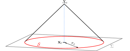
Figure 1: $2+1$ illustration for the relativistic location algorithm in the case of a spacelike configuration hyperplane $\Sigma$ in an adapted frame. If the configuration hyperplane $\Sigma$ is spacelike, then one can perform a Lorentz transformation so that the emission points lie on a surface of constant time coordinate $t=X^{\prime 0}$ (the corresponding $t$ axis is vertical) with a value $t=t_{0}$. In this frame, the emission points lie on a sphere $\mathcal{S}$ (represented here as a circle) in the configuration hyperplane $\Sigma$. The problem consists of first finding the circumcenter ${\bf x}_{\rm c}$ and the circumradius $r_{\rm c}$. In this frame, the time it takes for light to travel the distance $r_{\rm c}$ is $\Delta t=r_{\rm c}$ in units where the speed of light is unity. The intersection point is then given by $X_{\rm c}=\left(t_{0}+\Delta t,{\bf x}_{\rm c}\right)$.

II.2.1 Spacelike configuration hyperplane

We first consider the case where the configuration hyperplane $\Sigma$ is spacelike, so that the normal vector is timelike. In this case, one may write:

$$n=\left(\gamma,\beta\hat{r}\right),$$ (7)

where $\hat{r}=(\hat{r}_{x},\hat{r}_{y},\hat{r}_{z})$ is a unit vector. $\gamma:=n^{0}$ and $\beta=\sqrt{1-1/\gamma^{2}}$. One may then perform a Lorentz transformation to a frame in which the spatial components of the unit normal $n$ vanish. The Lorentz transformation matrix takes the form

$$\Lambda=\left[\begin{array}[]{cccc}\gamma&-\beta\gamma\hat{r}\\ -\beta\gamma\hat{r}&(I+(\gamma-1)\,\hat{r}\otimes\hat{r})\\ \end{array}\right],$$ (8)

where $I$ is the identity matrix and $\otimes$ denotes a tensor product.

Since the Lorentz transformation $\Lambda$ transforms to a frame in which $n^{\prime}=\Lambda\cdot n$ has no spatial components, it follows that since the vectors $E_{1}$, $E_{2}$, and $E_{3}$ are orthogonal to $n$, the time component of their transformed counterparts $E^{\prime}_{1}$, $E^{\prime}_{2}$, and $E^{\prime}_{3}$ must vanish. From Eq. (4), it follows that the time components of the transformed emission points $\underline{X}^{\prime}=\{X^{\prime}_{1},X^{\prime}_{2},X^{\prime}_{3},X^{\prime}_{4}\}$ are all equal; in this frame, the emission points all lie on the same constant time slice $t=t_{0}$. The primed frame will be called $\mathcal{B}$.

The problem of finding the intersection point of the light cones from four points is simply a matter of finding the point spatially equidistant from the four emission points. To see this, consider four signals emitted from four points at the same instant. We seek the spatial point at which the signals simultaneously arrive. The preceding analysis establishes that one can find a reference frame (frame $\mathcal{B}$) where the four emission points all lie on the same time slice. Since the speed of light is constant in all frames, the point where the signals simultaneously arrive must be spatially equidistant from the four emission points. If the distance between the simultaneous arrival point and each of the emission points is $r_{\rm c}$, then the time coordinate in frame $\mathcal{B}$ is given by the time it takes for light to travel a distance $r_{\rm c}$ (which has a value $r_{\rm c}$ in units where the speed of light is $c=1$).

In a three-dimensional Euclidean space, this is a straightforward task. Generically, four points that do not all lie in the same plane form the corners of a tetrahedron. It is well known that, for any tetrahedron, one can construct a circumsphere $\mathcal{S}$ that passes through all the corners of a tetrahedron. The coordinates of the circumcenter $\textbf{x}_{\rm c}$ specify the spatial coordinates of the intersection point in frame $\mathcal{B}$, and the circumradius determines the time coordinate. Given four (spatial) points $\{\textbf{x}_{1},\textbf{x}_{2},\textbf{x}_{3},\textbf{x}_{4}\}$, one can compute the coordinates of the circumcenter $\textbf{x}_{\rm c}$ using the following formulas Lévy and Liu (2010):

$$\textbf{x}_{\rm c}=\textbf{A}^{-1}{\bf u},$$ (9)

where the $3\times 3$ matrix A and the vector ${\bf u}$ are defined as

$$\textbf{A}:=\left[\begin{array}[]{c}\,[\textbf{x}_{2}-\textbf{x}_{1}]^{T}\\ \,[\textbf{x}_{3}-\textbf{x}_{1}]^{T}\\ \,[\textbf{x}_{4}-\textbf{x}_{1}]^{T}\end{array}\right]\qquad{\bf u}:=\frac{1}{2}\left[\begin{array}[]{c}\textbf{x}_{2}^{2}-\textbf{x}_{1}^{2}\\ \textbf{x}_{3}^{2}-\textbf{x}_{1}^{2}\\ \textbf{x}_{4}^{2}-\textbf{x}_{1}^{2}\end{array}\right].$$ (10)

The circumradius $r_{\rm c}$ may then be computed using the formula:

$$r_{\rm c}=|\textbf{x}_{\rm c}-\textbf{x}_{I}|^{1/2}.$$ (11)

The intersection of light cones in the frame $\mathcal{B}$ is then given by:

$$X^{\prime}_{\rm c}=\left(t_{0}+r_{\rm c},\textbf{x}_{\rm c}\right).$$ (12)

To obtain the intersection of the light cones $X_{\rm c}$ in the original frame $\mathcal{A}$, simply invert the Lorentz transformation:

$$X_{\rm c}=\Lambda^{-1}X^{\prime}_{\rm c}.$$ (13)

There are instances in which this algorithm fails. For instance, the algorithm may fail when the matrix $\bf{A}$ becomes degenerate, which can occur if the emission points are collinear or coplanar (in which case $r_{\rm c}$ diverges) Coll et al. (2012); these cases are discussed in detail in Abel and Chaffee (1991); Chaffee and Abel (1994).

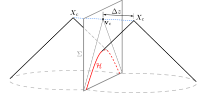
Figure 2: $2+1$ illustration for the relativistic location algorithm in the case of a timelike configuration hyperplane $\Sigma$ in an adapted frame (as in Fig. 1, the $t$ axis is vertical). If $\Sigma$ is timelike, then one can perform a Lorentz transformation so that the emission points lie on a surface of constant coordinate $z=X^{\prime 3}$, with the value $z=z_{0}$. In this frame, the emission points lie on a hyperboloid $\mathcal{H}$ (represented here as a hyperbola). The problem consists of first finding the coordinates of the vertex ${\bf v}_{\rm c}$ in this frame and the distance $R$, the latter being the distance between the vertex ${\bf v}_{\rm c}$ and a point on $\mathcal{H}$. The distance between the $z=z_{0}$ plane and the intersection point $X_{\rm c}$ is given by $R=\Delta z$. With these quantities in hand, one may obtain the intersection point $X_{\rm c}=\left({\bf v}_{\rm c},z_{0}\pm\Delta z\right)$.

II.2.2 Timelike configuration hyperplane

We now turn to the case in which the configuration hyperplane $\Sigma$ is timelike, which corresponds to a spacelike unit normal vector $n^{\mu}$. In this case, the adapted frame is constructed differently; one first performs a Lorentz transformation such that the spacelike $n^{\mu}$ is tangent to a surface of constant $t=X^{\prime 0}$ (here, $t=X^{\prime 0}$, $x=X^{\prime 1}$, $y=X^{\prime 2}$, $z=X^{\prime 3}$). Then, one performs a spatial rotation so that $n^{\mu}$ is aligned with the $z$ axis. The configuration hyperplane $\Sigma$ in the resulting frame is characterized by a constant $z=z_{0}$ coordinate. The points will lie on an elliptic hyperboloid $\mathcal{H}$ formed by the intersection of the past light cone for the solution point and the configuration hyperplane $\Sigma$ (see Fig. 2). The main task is to find the coordinates for the vertex ${\bf v}_{\rm c}=\left(t_{\rm c},x_{\rm c},y_{\rm c}\right)$ of the cone which the hyperboloid asymptotes to, as well as the distance $R$ satisfying the following set of equations:

$$\Phi_{I}=-R^{2},$$ (14)

where

$$\Phi_{I}:=\left(x_{I}-x_{\rm c}\right)^{2}+\left(y_{I}-y_{\rm c}\right)^{2}-\left(t_{I}-t_{\rm c}\right)^{2}.$$ (15)

By eliminating $R$, one may write this as a set of three equations:

$$\Phi_{1}=\Phi_{2}$$ (16)

$$\Phi_{2}=\Phi_{3}$$

$$\Phi_{3}=\Phi_{4},$$

which can then be solved for the vertex coordinates ${\bf v}_{\rm c}$ by way of a computer algebra system (we use Mathematica Inc. to obtain explicit expressions).

The vertex coordinates provide the $\left(t,x,y\right)$ coordinates for the intersection of future pointing light cones. The $z$ coordinate for the intersection of light cones is given by

$$z_{\rm c}=z_{0}\pm R.$$ (17)

In this case, one does not have a unique point for the intersection of light cones—this is the bifurcation problem, which is discussed in detail in Coll et al. (2012).

II.3 Unified four emission point formula

It is also possible to calculate the intersection point $X_{\rm c}$ using a closed-form formula that applies regardless of the geometrical configuration of the four emission points. Such a formula was presented in Coll et al. (2010b, 2012) and it is given by

$$X_{\rm c}^{\mu}= X_{1}^{\mu}+y_{*}^{\mu}-\frac{y^{\nu}_{*}y_{*\nu}N^{\mu}}{y^{\sigma}_{*}N_{\sigma}\pm\sqrt{|(y^{\sigma}_{*}N_{\sigma})^{2}-y^{\sigma}_{*}y_{*\sigma}N^{\tau}N_{\tau})|}},$$ (18)

where $X_{1}^{\mu}$ is one of the emission points, $N^{\mu}$ is defined in Eq. (5), and $y_{*}^{\mu}$ is given by

$$y_{*}^{\mu}:=\frac{1}{\xi^{\nu}N_{\nu}}(i_{\xi}H)^{\mu}.$$ (19)

Here, $\xi$ is any vector satisfying $\xi^{\mu}N_{\mu}\neq 0$, and $i_{\xi}H$ is the interior product of $\xi$ and the two form $H$ [explicitly $(i_{\xi}H)^{\mu}=\eta^{\mu\nu}\xi^{\sigma}H_{\sigma\nu}$]. Given the definition for the frame vectors in Eq. (4), the two-form $H$ may be expressed as:

$$H:=\Omega_{1}h(E_{2},E_{3})+\Omega_{2}h(E_{3},E_{1})+\Omega_{3}h(E_{1},E_{2}),$$ (20)

$$\Omega_{i}:=\eta_{\mu\nu}E^{\mu}_{i}E^{\nu}_{i},\qquad h(U,V)_{\alpha\beta}:=-\varepsilon_{\alpha\beta\mu\nu}U^{\mu}V^{\nu},$$

with no sum on $i$ in the expression for $\Omega_{i}$.

Note that the $\pm$ sign in (18) means that there are always two candidate solutions, even if the geometrical configuration leads to just one. This complicates a straightforward use of the formula. The determination of the correct sign is somewhat involved—especially when the bifurcation problem mentioned in the previous section is present Coll et al. (2012).

II.4 Five emission points

The bifurcation problem may be solved most easily by including an additional point. If five emission points are available, then one can obtain the intersection point in a straightforward way. Following Ruggiero et al. (2022), one begins with the constraint function:

$$\Psi_{I}:=\left(X_{I}^{\mu}-X_{\rm c}^{\mu}\right)\left(X_{I}^{\nu}-X_{\rm c}^{\nu}\right)\eta_{\mu\nu},$$ (21)

where now $I\in\{1,2,3,4,5\}$. One can take the differences to form four unique equations of the following form:

$$\Psi_{I}-\Psi_{J}=\eta_{\mu\nu}\left[2\,X_{\rm c}^{\mu}\left(X_{J}^{\nu}-X_{I}^{\nu}\right)+X_{I}^{\mu}\,X_{I}^{\nu}-X_{J}^{\mu}\,X_{J}^{\nu}\right],$$ (22)

which are linear in $X_{\rm c}^{\mu}$; one can reduce this to a straightforward linear algebra problem, provided that the matrix $X_{J}^{\nu}-X_{I}^{\nu}$ of emission point differences is nondegenerate. One may observe that the matrix of emission point differences becomes degenerate when any two emission points are brought together—for this reason, one might encounter a loss of precision for closely separated emission points. Though this formula requires an additional emission point, it is preferred due to its computational simplicity and accuracy.

II.5 Implementation, evaluation, and discussion

The new algorithms we have presented here, as well as the formulas described in Coll et al. (2010b, 2012) and the five-point algorithm of Ruggiero et al. (2022) [which we have described in Eqs. (21) and (22)], have been implemented in the cereal.jl code, available at Feng et al. (2022a). We have written cereal.jl to accommodate abstract datatypes; this allows user-specified floating point precision. In the tests we perform, we consider two types of floating point variables, the default Float64 double precision, and the Double64 “double double” precision variables implemented in the DoubleFloats library J. Sarnoff, et al. (2018).

Included in cereal.jl are test routines that perform tests of the code by stochastically generating a set of $N$ emission points on the past light cone of some intersection point $X_{\rm c}$, and comparing the results $X_{\rm r}$ generated by the algorithms in cereal.jl with the true value for $X_{\rm c}$. The points $X_{\rm c}$ and $X_{\rm r}$ are compared according to Euclidean $L_{2}$ norms (with $|V|=\sqrt{V\cdot V}$ for some vector $V$):

$$\varepsilon=|X_{\rm r}-X_{\rm c}|/|X_{\rm c}|$$ (23)

In our tests, the most accurate algorithm is the five-point formula of Ruggiero et al. (2022), which for $10^{6}$ test cases satisfies $\varepsilon<10^{-9}$ with double precision (Float64), and $\varepsilon<10^{-23}$ with extended precision (Double64). The accuracy of the new algorithm presented in Sec. II.2 and the formula in Sec. II.3 Coll et al. (2010b, 2012) are comparable to each other, but both are less accurate than the formula of Ruggiero et al. (2022). For $10^{6}$ test cases, the errors for the four-point methods in Secs. II.2 and II.3 typically satisfy $\varepsilon<10^{-5}$ with double precision (Float64), and $\varepsilon<10^{-14}$ with extended precision (Double64).

Execution times differ greatly between the algorithms. On a standard desktop computer (with an Intel i5-7500 processor), the five-point formula of Ruggiero et al. (2022) typically performs the computation in $<1.5~{}\rm\mu s$. The four-point algorithms that we have implemented in cereal.jl are significantly slower, despite only requiring four emission points. For four emission points, our implementation of the formula in Coll et al. (2010b, 2012) typically requires $\sim 150~{}\rm\mu s$ to perform the computation. The algorithm we have presented here has improved performance, requiring a computation time of $\sim 36~{}\rm\mu s$. Since the five-point formula is faster and yields results with significantly higher accuracy, we employ it when computing the initial guess for the curved spacetime algorithm that we will describe in the next section.

We note that the algorithms described here may be used in conformally flat spacetimes, since flat spacetimes and conformally flat spacetimes share the same null cone and null geodesic structure on regions where the conformal factor remains nonsingular. In particular, the intersection point for four null cones in a conformally flat spacetime will be the same as that for the underlying flat spacetime (underlying in the sense that the metric for the conformally flat spacetime differs from the flat spacetime by a conformal factor). This class of spacetimes include cosmological spacetimes, such as de Sitter, anti-de Sitter and the more general Friedmann-Lemaitre-Robertson-Walker spacetimes.

III Relativistic location in curved spacetime

III.1 Geodesics

For general spacetime geometries, described by a metric tensor $g_{\mu\nu}$ and its inverse $g^{\mu\nu}$, the problem of finding the intersection point $X_{\rm c}$ of four future pointing light cones (provided that such a point exists) amounts to finding the intersection of four null geodesics from the emission points $\underline{X}$; this follows from the fact that for some emission point $X_{I}$, a point $X_{\rm p}$ in the future pointing null cone lies on a geodesic connecting $X_{\rm p}$ and $X_{I}$. Note also that the emission points $\underline{X}$ lie on the past light cone of $X_{\rm c}$. Given some inverse metric $g^{\mu\nu}=g^{\mu\nu}(x)$ describing the spacetime geometry, an affinely parametrized null geodesic may be described by the Hamiltonian

$$H:=\frac{1}{2}\,g^{\mu\nu}\,p_{\mu}\,p_{\nu},$$ (24)

where the four-momenta are given by

$$p_{\mu}=g_{\mu\nu}\frac{dx^{\nu}}{d\lambda},$$ (25)

and the associated Hamilton equations are

$$\frac{d{x}^{\mu}}{d\lambda}=\frac{\partial H}{\partial p_{\mu}},\qquad\qquad\frac{d{p}_{\mu}}{d\lambda}=-\frac{\partial H}{\partial x^{\mu}}.$$ (26)

For null geodesics, the initial data at $\lambda=0$ is given by an initial point ${x}_{0}^{\mu}$ and an initial three velocity ${\bf v}^{i}$, with the initial four-momentum $p_{\mu}|_{\lambda=0}$ satisfying the following (with $i\in\{1,2,3\}$):

$$\left.\delta{{}^{i}}{{}_{\mu}}\frac{dx^{\mu}}{d\lambda}\right|_{\lambda=0}={\bf v}^{i},\qquad\left.g_{\mu\nu}({x}_{0})\frac{dx^{\mu}}{d\lambda}\frac{dx^{\nu}}{d\lambda}\right|_{\lambda=0}=0.$$ (27)

The solution to Hamilton’s equations is formally given by $x^{\mu}=x^{\mu}(\lambda,{x}_{0},{\bf v})$. Since $\lambda$ is an affine parameter, one can redefine $\lambda$ up to linear transformations—it is therefore always possible to rescale $\lambda$ so that it takes values in the domain $\lambda\in[0,1]$, with $\lambda=1$ being the final point.

III.2 Geodesic intersection

The problem of finding the intersection of light cones in a slightly curved spacetime may be reformulated in terms of null geodesics Carloni et al. (2020). Consider four formal solutions to Hamilton’s equations (26), distinguished by the indices $I\in\{1,2,3,4\}$, that have end points ${\rm x}^{\mu}_{I}$ which are functions of the initial data ${X}_{I}$ and ${\bf v}_{I}$:

$${\rm x}^{\mu}_{I}={\rm x}^{\mu}_{I}({X}_{I},{\bf v}_{I})=x^{\mu}_{I}(1,{X}_{I},{\bf v}_{I}).$$ (28)

Then define the following vector valued function:

$$F:=\left({\rm x}_{1}-{\rm x}_{2},{\rm x}_{1}-{\rm x}_{3},{\rm x}_{1}-{\rm x}_{4}\right).$$ (29)

where $F=F(\underline{X},v)$ [with $v=({\bf v}_{1},{\bf v}_{2},{\bf v}_{3},{\bf v}_{4})$]. Observe that upon evaluation, the function $F$ yields a 12 component vector. The intersection of four null geodesics is given by the condition

$$F(\underline{X},v)=0.$$ (30)

The problem of solving the system of 12 equations in Eq. (30) is a standard root-finding problem. In particular, given a set of four emission points $\underline{X}=\{X_{1},X_{2},X_{3},X_{4}\}$, one solves Eq. (30) for the 12 quantities $v=({\bf v}_{1},{\bf v}_{2},{\bf v}_{3},{\bf v}_{4})$ that constitute the initial data.

III.3 Initial data

From here on, we write $f(v)=F(\underline{X},v)$ for simplicity, suppressing the dependence on emission points $\underline{X}$. The specific root finding algorithm we intend to employ will be based on an iterative quasi-Newton method, which requires an initial guess. It is therefore appropriate to begin by assuming that the spacetime geometry is slightly curved; the flat spacetime algorithms described earlier may then be used to construct an initial guess for $v$.

Initial data for the geodesics is constructed from the emission points $\underline{X}=\{X_{1},X_{2},X_{3},X_{4}\}$ and the flat spacetime intersection point $X_{\rm c}$. From these, one obtains the initial guess for the vector $v=({\bf v}_{1},{\bf v}_{2},{\bf v}_{3},{\bf v}_{4})$:

$${\bf v}^{i}_{I}:=X^{i}_{\rm c}-X^{i}_{I},$$ (31)

in units of dimensionless affine parameter. From $v$ and $\underline{X}$, one may construct the initial data for the geodesics by first constructing the vector $V_{I}$ for each geodesic:

$$V_{I}=\left(V^{0}_{I},{\bf v}^{1}_{I},{\bf v}^{2}_{I},{\bf v}^{3}_{I}\right),$$ (32)

where $V^{0}_{I}$ is determined by the condition

$$V^{\mu}_{I}\,V^{\nu}_{I}\,g_{\mu\nu}(X_{I})=0.$$ (33)

The conjugate momenta are given by

$$p^{I}_{\mu}=V^{\nu}_{I}\,g_{\mu\nu}(X_{I}).$$ (34)

The initial positions $X_{I}$ and initial conjugate momenta $p^{I}$ provide initial data for Eq. (26), which may then be solved to compute the value of $f(v)$ according to Eq. (29).

III.4 Root finding

In general, one does not possess analytical solutions to the geodesic equation (26) for a generic metric $g_{\mu\nu}$. To evaluate the function (29), one must therefore solve the geodesic equation (26) numerically for each emission point. One might expect a root finding algorithm for Eq. (30) to be computationally expensive, particularly in the computation of a Jacobian.

However, libraries for efficiently computing the Jacobian of generic functions have become available in recent years, in particular those that employ automatic differentiation methods. Automatic differentiation refers to a set of methods which, by way of the chain rule, exploit the fact that all numerical computations can in principle be broken down into finite compositions of elementary arithmetic operations. These methods can in principle be used to numerically compute the derivatives of programs to machine precision with a minimal computational overhead. A detailed discussion of automatic differentiation may be found in Neidinger (2010); Baydin et al. (2018). In our approach, we obtain the Jacobian of $=F(\underline{X},v)$ by automatic differentiation of numerical solutions to the geodesic equation in a generic slightly curved spacetime.

The specific root finding algorithm we employ is based on an iterative quasi-Newton Broyden method Broyden (1965); Press et al. (2007), which we summarize here. The task at hand is to obtain the root of some function $f(v)$. In the initial iteration, the Jacobian of $f(v)$ is computed using automatic differentiation methods. We also employ automatic differentiation in computing the gradient of the Hamiltonian, a strategy also employed in Christian, P. and Chan, C. -K. (2021) for solving the geodesic equation in Hamiltonian form. Given the Jacobian ${\bf J}$ and its inverse ${\bf J}^{-1}$, at some iteration ${\rm i}$, one can update $v$ according to the Newton prescription:

$$v_{{\rm i}+1}=v_{\rm i}+{\bf J}^{-1}_{{\rm i}}f(v_{\rm i}).$$ (35)

In the standard Broyden method (alternatively referred to as the “good” Broyden method), the first iteration is given by Eq. (35), with the Jacobian computed by differentiation. For the subsequent iterations, one computes the following:

$$\Delta v_{\rm i} =v_{\rm i}-v_{{\rm i}-1}$$ (36)

$$\Delta f_{\rm i} =f(v_{\rm i})-f(v_{{\rm i}-1}),$$

The inverse Jacobian ${\bf J}^{-1}$ is then updated according to the Sherman-Morrison formula:

$${\bf J}^{-1}_{{\rm i}+1}={\bf J}^{-1}_{\rm i}+\frac{\Delta v^{T}_{\rm i}-{\bf J}^{-1}_{\rm i}\,\Delta f_{\rm i}}{\Delta v^{T}_{\rm i}\,{\bf J}^{-1}_{\rm i}\,\Delta f_{\rm i}}\Delta v^{T}_{\rm i}\,{\bf J}^{-1}_{\rm i}.$$ (37)

One may then use Eq. (37) in conjunction with (35) to iteratively solve for the root of $f(v)$. The termination of the algorithm is determined by the behavior of $f_{\rm i}$; if a local minimum is detected within a specified range of iterations, the algorithm terminates and the results corresponding to the minimum are returned. In case the algorithm does not converge, a hard termination limit is used.

Given a root for $f(v)$, one can obtain the intersection point by solving the geodesic equations once more with the updated values for the initial data constructed from $v$ and $\underline{X}$, and averaging over the end points (which are assumed to be close).

III.5 The squirrel algorithm

We now summarize the curved spacetime algorithm employed in the squirrel.jl code:

1. First, apply a flat spacetime algorithm (either that of Secs. II.2 or II.4) to the emission points $\underline{X}$ to obtain a guess for the intersection point and initial velocities.

2. Apply a root finding algorithm to the function $f(v)=F(\underline{X},v)$ to obtain the initial velocities $v$ for subsets of four emission points.

3. Integrate the geodesics with the resulting initial velocities $v$ and emission points $\underline{X}$ to find the intersection point.

As indicated, steps 2 and 3 of the above algorithm are applied to a subset of four emission points. If additional emission points are available, an outlier algorithm, described in the next subsection, is employed to exclude large errors.

III.6 Outlier detection

There are instances in which the algorithm described in this section can generate large errors, which can result from a combination of large errors in the initial guesses provided by the flat spacetime algorithm and convergence failures in the Broyden algorithm. One might expect such errors to occur, since the function $F(\underline{X},v)$ is generally nonlinear. To increase the reliability of the algorithm, we describe here methods that can mitigate the effects of these errors when additional emission points are available.

As discussed before, given $N>4$ emission points, one can choose up to $C(N,4)$ combinations of four emission points $\underline{X}$, and for each set $\underline{X}$, the previously described algorithm can be applied to obtain a total of $C(N,4)$ intersection points. Since there is only one receiver for the emission data, all $C(N,4)$ intersection points should agree. If errors in the algorithm are assumed to be rare, one can employ an outlier detection algorithm that can identify the intersection points that strongly deviate from the others.

We employ a simple outlier detection algorithm, which begins by first computing the median values for the intersection points, and then computes the deviation of each intersection point from the median. The points which deviate from the median beyond a user-specified threshold are then discarded. The final intersection point is then computed from the remaining intersection points.

III.7 Remarks on implementation

The algorithm described here is implemented in the squirrel.jl code (available at Feng et al. (2022b)). The squirrel.jl code is written in the Julia language, which is ideal for implementing the squirrel algorithm due to the state of the art automatic differentiation and ODE solver libraries available. Automatic differentiation is handled using the ForwardDiff.jl forward-mode automatic differentiation library Revels et al. (2016), and geodesics are integrated using the recommended Verner seventh order Runge-Kutta integrator AutoVern7 Verner (2010) in OrdinaryDiffEq.jl Rackauckas and Nie (2017), which features stiffness detection and automated switching to a specified stiff integrator (we use the fifth order Rosenbrock method integrator Rodas5 Di Marzo (1993)). Though our system is Hamiltonian, we have avoided symplectic integrators in favor of integrators with adaptive time stepping in order to minimize execution time.

The Broyden algorithm is implemented directly, depending only on standard Julia libraries. The default termination limit is set to $24$. The initial guess is provided by one of the flat spacetime algorithms implemented in the cereal.jl code, depending on the number of emission points available; if $N=4$ emission points are available, then the flat spacetime algorithm presented in Sec. II.2 is employed (in which case, our implementation returns two points), but if $N\geq 5$ emission points are available, then the formula of Ruggiero et al. (2022) reviewed in Sec. II.4 is employed. The outlier detection algorithm becomes active for $N\geq 5$ emission points, and is applied to the location algorithm of squirrel.jl to remove results with large errors.

Since there is now widespread availability of devices with multithreading capabilities, the squirrel.jl code employs multithreading on loops containing the integration of geodesics and the automatic differentiation of geodesic solutions. With multithreading enabled on a desktop computer with four cores and four threads (Intel i5-7500), the squirrel.jl code can establish a position from five emission points in under $1~{}{\rm s}$ for reasonably simple spacetime geometries—benchmarks will be discussed in Sec. VI.3.

IV Curved spacetime geometries

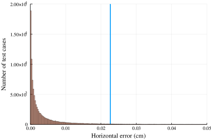
Figure 3: Horizontal positioning errors for our implementation of the five emission point algorithm of Ruggiero et al. (2022) relative to the Kerr-Schild geometry for $10^{5}$ test cases. The closely spaced vertical lines correspond to the rms values and $95\%$ confidence level for the errors, with respective values of $0.0226$ and $0.0227~{}{\rm cm}$. Out of $10^{5}$ samples, two samples ($0.002\%$) have an error $>2~{}{\rm cm}$ with the largest error being $3.3~{}{\rm cm}$.

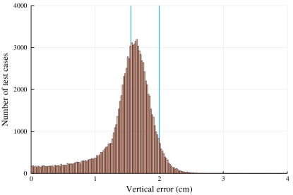
Figure 4: Vertical positioning errors for our implementation of the five emission point algorithm of Ruggiero et al. (2022) relative to the Kerr-Schild geometry for $10^{5}$ test cases. The vertical lines correspond to the rms values and $95\%$ confidence level for the errors, with respective values of $1.56$ and $2.00~{}{\rm cm}$. Out of $10^{5}$ samples, $11$ samples ($0.011\%$) have an error $>5~{}{\rm cm}$ with the largest error being $15.0~{}{\rm cm}$.

IV.1 The Kerr-Schild metric

In this section, we describe some specific choices for the spacetime metric $g_{\mu\nu}$ used in our tests. In general relativity, the spacetime geometry surrounding a stationary rotating object in a vacuum is given by the Kerr geometry Kerr (1963), described by the following metric in Kerr-Schild coordinates Kerr and Schild (2009):

$$g_{\mu\nu} =\eta_{\mu\nu}+f\,k_{\mu}\,k_{\nu},$$ (38)

$$k_{\mu} =\left(1,\frac{r\,x+a\,y}{r^{2}+a^{2}},\frac{r\,y-a\,x}{r^{2}+a^{2}},\frac{z}{r}\right),$$

$$f =\frac{2\,G\,M\,r^{3}}{r^{4}+a^{2}\,z^{2}},$$

where $G$ is the gravitational constant, $M$ is the mass, and $a$ is the spin parameter. The radius $r$ may be compactly expressed as the solution to

$$\frac{x^{2}+y^{2}}{r^{2}+a^{2}}+\frac{z^{2}}{r^{2}}=1.$$ (39)

At the surface of the Earth, the spacetime curvature is small, so one might ask whether the flat spacetime algorithms suffice for positioning, neglecting tropospheric and ionospheric corrections. To determine whether this is indeed the case, we test the five-point algorithm in Eqs. (21) and (22) against the Kerr geometry. Recalling that emission points lie on the past light cone of the intersection point $X_{\rm c}$, we stochastically generate intersection points $X_{\rm c}$, then construct initial data for past directed null geodesics. To obtain the emission points $\underline{X}=\{X_{1},X_{2},X_{3},X_{4},X_{5}\}$, we integrate the geodesic Hamilton equations for five sets of initial data for the null geodesics. The resulting emission points $\underline{X}$ are used with the formula of Ruggiero et al. (2022) to obtain $X_{\rm c}$, the intersection point in flat spacetime. The positioning error is given by (with vertical bars denoting the $L_{2}$ Euclidean distance norm)

$$\epsilon_{\rm KSc}=|\hat{P}({\bf x}_{\rm tar}-{\bf x}_{\rm c})|.$$ (40)

Here, $\hat{P}(\cdot)$ is a projection operator (projecting to horizontal or vertical directions relative to some surface), ${\bf x}_{\rm c}$ form the spatial components of $X_{\rm c}$, and ${\bf x}_{\rm tar}$ denotes the spatial components of $X_{\rm tar}$ which is the true intersection point for the future light cones of $\underline{X}$ with respect to the Kerr-Schild metric.

We consider a Kerr-Schild metric with parameter choices $GM=1$ and $a=738$ (the latter corresponding to the angular momentum for the Earth). We perform a test with $10^{5}$ randomly generated target points $X_{\rm tar}$ on the WGS-84 reference ellipsoid Imagery and Agency (2000) (setting $M$ to be the Earth mass) and randomly generated initial datasets for null geodesics. The result, illustrated in Figs. 3 and 4, indicates that the error satisfies $\epsilon_{\rm KSc}\leq 2~{}{\rm cm}$ for $95\%$ of the points in the vertical direction (the direction orthogonal to the reference ellipsoid), and $\epsilon_{\rm KSc}\leq 3~{}{\rm mm}$ in the horizontal direction. In a vacuum, the five emission point algorithm in flat spacetime suffices for positioning to an accuracy on the order of a centimeter. This result is consistent with those of Puchades and Sáez (2016), where it is also argued that the dominant errors from spacetime curvature come from the determination of satellite orbits, rather than the bending of photon trajectories.

IV.2 The Gordon metric

If one seeks centimeter-scale accuracy in a vacuum on terrestrial scales, then flat spacetime algorithms suffice. However, for terrestrial positioning, tropospheric and ionospheric effects significantly affect the propagation of electromagnetic signals and introduce errors in the computed position. From a general relativistic perspective, one might be tempted to dismiss tropospheric and ionospheric effects as ancillary (practical considerations aside), as the underlying spacetime geometry does not depend to a significant degree on tropospheric and ionospheric profiles. However, in a positioning system based on the exchange of electromagnetic signals, such effects will deform the emission coordinates, and, in this sense, tropospheric and ionospheric effects should still be taken into consideration even if one insists on a fundamentally relativistic approach.

Fortunately, as indicated in Tarantola et al. (2009), the framework of general relativity can by way of analog spacetime geometries incorporate the effects of dielectric media on electromagnetic signal propagation. In dielectric media, light propagation may under certain conditions be described with the geodesics of the Gordon metric Gordon (1923); Pham (1956); Barceló et al. (2005), which has the form

$$\bar{g}_{\mu\nu} =g_{\mu\nu}+\left(1-\frac{1}{n^{2}}\right)u_{\mu}u_{\nu},$$ (41)

where $u^{\mu}$ corresponds to the four-velocity of the medium, and $n$ is an effective index of refraction. To simplify the analysis, we will neglect the rotation of the Earth (in general, the corotation of the medium can be included through the four-velocity $u^{\mu}$). The tropospheric index of refraction has a sea level value of $n_{\rm atm}-1\sim 2.7\times 10^{-4}$, and the effective index of refraction for the ionosphere has a maximum value on the order of $n_{\rm ion}-1\sim 4.0\times 10^{-5}$. It follows that the tropospheric and ionospheric corrections to the metric are of the respective orders $10^{-4}$ and $10^{-5}$. In contrast, the difference $f\,k_{\mu}\,k_{\nu}$ between the components of the Kerr-Schild metric and the Minkowski metric is roughly on the order of $10^{-9}$ at the surface of the Earth, so tropospheric and ionospheric effects dominate.

IV.3 Weak field metric

At this point we emphasize that when performing tests with the analog Gordon metric, we incorporate gravitational effects with the weak-field metric, rather than the Kerr metric. The weak field metric has the form

$$g_{\mu\nu}=\eta_{\mu\nu}-2\,V\,\delta_{\mu\nu},$$ (42)

where $V$ is the gravitational potential of the Earth, which takes the form

$$V=-\frac{GM}{r}\left[1-J_{2}\left(\frac{a_{\rm ell}^{2}}{r^{2}}P_{2}(\cos\theta)\right)\right],$$ (43)

where $r^{2}=x^{2}+y^{2}+z^{2}$, $P_{2}$ is a Legendre polynomial of degree $2$, $J_{2}$ is a quadrupole moment of the Earth, which takes a value of Ashby (2003)

$$J_{2}=1.0826300\times 10^{-3}.$$ (44)

The quantity $a_{\rm ell}$ is the equatorial radius of the Earth, and is one of the parameters of the reference ellipsoid, which approximates the Earth’s geoid up to roughly $100~{}{\rm m}$. Following Ashby (2003), the reference ellipsoid we use is the WGS-84 standard Imagery and Agency (2000), which corresponds to the following values for the semimajor axis $a_{\rm ell}$ and the semiminor axis $b_{\rm ell}$:

$$a_{\rm ell} =6378.137~{}{\rm km},$$ (45)

$$b_{\rm ell} =6356.752314245~{}{\rm km}.$$

V Index of refraction models

We now turn to the construction of models for the effective index of refraction, which we will use in the analog Gordon metric (41) for our tests of the algorithm. The effective index of refraction is then given by the following expression

$$n_{\rm eff}=1+\Delta n_{\rm atm}+\Delta n_{\rm ion}.$$ (46)

In this section, we describe the construction of simplified profiles for $\Delta n_{\rm atm}$ and $\Delta n_{\rm ion}$ which we will use in evaluating the squirrel.jl code.

V.1 Atmospheric model

Given the pressure and temperature profiles for the atmosphere, the profile for the atmospheric index of refraction (here excluding contributions from the ionosphere) can be computed from the revised Edlén equation Birch and Downs (1993); *Edlen1966 for the refractive index of air:

$$\Delta n_{\rm air}= \frac{\Delta n_{\rm s}\left[P/{\rm Pa}\right]}{96095.43}$$ (47)

$$\times\frac{1+10^{-8}\left(0.601-0.00972\left[T/^{\circ}{\rm C}\right]\right)\left[P/{\rm Pa}\right]}{1+0.0036610\left[T/^{\circ}{\rm C}\right]},$$

where $\Delta n_{\rm air}=n_{\rm air}-1$, and $\Delta n_{\rm s}$ is given by

$$\Delta n_{\rm s}\times 10^{8}= 8342.54+\frac{2406147}{130-1/\lambda^{2}}+\frac{15998}{38.9-1/\lambda^{2}}.$$ (48)

Following Vasylyev et al. (2019), one may obtain standard atmospheric temperature and pressure profiles from one of several atmospheric models, for instance the U.S. Standard Atmosphere model Atm , or the more detailed NRLMSISE-00 model Picone et al. (2002). Using the former, atmospheric index of refraction profiles up to $80~{}{\rm km}$ are computed, and we fit the computed values to a function of the form:

$$\Delta n_{\rm atm}=\frac{A_{1}}{B_{1}+C_{1}\left(h-H_{1})\right)}+\frac{A_{2}}{B_{2}+C_{2}\left([h]-H_{2})\right)},$$ (49)

with $h$ denoting altitude (in ${\rm km}$) from an appropriate reference ellipsoid. The fitted parameter values are

$$A_{1} =-222.666, \qquad A_{2} =-253.499,$$ (50)

$$B_{1} =99.0621, \qquad B_{2} =112.757,$$

$$C_{1} =0.157823~{}{\rm km}^{-1}, \qquad C_{2} =0.179669~{}{\rm km}^{-1},$$

$$H_{1} =-7.1541~{}{\rm km}, \qquad H_{2} =-7.15654~{}{\rm km}.$$

Though it would be aesthetically preferable to employ exponential functions in our model, we refrain from using them to avoid potential instabilities in the libraries we used for the integration of ODEs. Since the contributions from $\Delta n_{\rm atm}$ are concentrated in the troposphere, the contributions from $\Delta n_{\rm atm}$ will be referred to as tropospheric.

V.2 Ionospheric model

The effective index of refraction for electromagnetic wave propagation the ionosphere is given by the Appleton–Hartree equation Bittencourt (2004); Appleton (1932); *Hartree1931. We consider here an approximation which assumes a collisionless plasma, and signal frequencies $\omega:=2\pi f$ much greater than the gyrofrequency $\omega_{\rm g}:=|q{\bf b}_{\rm E}/m_{\rm e}|$ with ${\bf b}_{\rm E}$ being the Earth’s magnetic field, and $q$, $m_{\rm e}$ being the respective charge and mass of the electron. For GNSS signals, $f\sim 10^{9}~{}{\rm Hz}$, and $\omega_{\rm g}/\omega\approx 3\times 10^{-3}$, so this approximation is reasonable. The corrections to the effective index of refraction $n_{\rm ion}$ from the gyrofrequency are in fact proportional to $\omega_{\rm g}/\omega$, and depend on the angle between the direction of radio wave propagation and ${\bf b}_{\rm E}$. If gyrofrequency corrections become important, nongeometrical corrections to the geodesic equation may be needed, in which case the Gordon metric alone does not suffice for characterizing the propagation of electromagnetic signals. However, one may nonetheless suppress such corrections with higher signal frequencies.

Under the assumptions in the preceding paragraph, the Appleton-Hartree formula for the ionospheric phase index of refraction $n_{\rm ph}$ may be approximated as

$$\Delta n_{\rm ph}\approx-\frac{\omega_{\rm p}^{2}}{f^{2}}=-\left(4.024\times 10^{-17}\right)[N_{\rm e}/{\rm m}^{-3}],$$ (51)

where $\Delta n_{\rm ph}=n_{\rm ph}-1$, and $\omega_{\rm p}^{2}=q^{2}N_{\rm e}/2\epsilon_{0}\,m_{\rm e}$ is the squared plasma frequency, with $\epsilon_{0}$ being the vacuum permittivity, and $N_{\rm e}$ the electron density in ${\rm m}^{-3}$. Since the corrections from the gyrofrequency $\omega_{\rm g}$ are linear, we assume that the index $\Delta n_{\rm ph}$ can only be modeled up to a precision of $0.3\%$ for signals in the GHz range. It should be mentioned that since $n_{\rm ph}<1$, $n_{\rm ph}$ can only be the index of refraction associated with the phase velocity. To obtain the index of refraction associated with the group velocity, one employs the dispersion relation $\omega^{2}=k^{2}+\omega_{\rm p}^{2}$ for cold, collisionless plasmas Bittencourt (2004) to obtain the following expression for the group index of refraction (with $\Delta n_{\rm ion}=n_{\rm ion}-1$)

$$\Delta n_{\rm ion}\approx-\Delta n_{\rm ph}.$$ (52)

The electron density $N_{\rm e}$ can be determined by measurement and modeling; the Global Positioning System employs the Klobuchar model Klobuchar (1987) and the Galileo GNSS makes use of the NeQuick-G ionospheric model detailed in European Union (2016b) (which is a revised version of the NeQuick model in Radicella and Leitinger (2001)). In these models, the ionospheric profile is described in terms of the dimensionless Epstein function:

$$Ep(h,h_{\rm c},B):=\frac{4\exp\left(\frac{h-h_{\rm c}}{B}\right)}{\left(\exp\left(\frac{h-h_{\rm c}}{B}\right)+1\right)^{2}},$$ (53)

which has the form of a line shape function. One may approximate the above with the pseudo-Epstein function:

$$\tilde{E}p(h,h_{\rm c},B):= \frac{1}{16}\biggl{\{}\left[1+\left(\tfrac{h-h_{\rm c}}{2B}\right)^{2}\right]^{-1}+\left[1+\left(\tfrac{h-h_{\rm c}}{4B}\right)^{2}\right]^{-2}$$ (54)

$$+\left[1+\left(\tfrac{h-h_{\rm c}}{6B}\right)^{2}\right]^{-3}+\left[1+\left(\tfrac{h-h_{\rm c}}{7B}\right)^{2}\right]^{-4}\biggr{\}}^{2},$$

which differs from the Epstein function by roughly one part in $10^{3}$; this suffices, since the approximation for the Appleton–Hartree equation is only valid to $3\times 10^{-3}$ for GNSS signal frequencies.

For simplicity, we construct a simple model for the electron density $N_{\rm e}$ consisting of a sum of pseudo-Epstein functions:

$$N_{\rm e}:= \biggl{[}\alpha_{\rm D}\,\tilde{E}p(h,h_{\rm D},b_{\rm D})+\alpha_{\rm E}\,\tilde{E}p(h,h_{\rm E},b_{\rm E})$$ (55)

$$\>\>+\alpha_{\rm F}\,\tilde{E}p(h,h_{\rm F},b_{\rm F})\biggr{]}.$$

The subscripts ${\rm D}$, ${\rm E}$, ${\rm F}$ on the parameters correspond to the respective ionospheric layers. Of course the precise profiles for the ionospheric layers are rather complicated and time dependent, depending on the time of day and calendar date; in practice, such detailed profiles are provided by the aforementioned ionospheric models (see for instance European Union (2016b) for a detailed description of the NeQuick-G model employed in the Galileo system). However, a simplified model for the ionospheric layers will suffice for demonstrating the viability of our algorithm. We choose the parameter values:

$$\alpha_{\rm D} =10^{12}~{}{\rm m}^{-3}, \quad h_{\rm D} =75~{}{\rm km}, \quad b_{\rm D} =5~{}{\rm km},$$ (56)

$$\alpha_{\rm E} =2.5\times 10^{11}~{}{\rm m}^{-3}, \quad h_{\rm E} =130~{}{\rm km}, \quad b_{\rm E} =30~{}{\rm km},$$

$$\alpha_{\rm F} =10^{11}~{}{\rm m}^{-3}, \quad h_{\rm F} =300~{}{\rm km}, \quad b_{\rm F} =50~{}{\rm km}.$$

V.3 Perturbation model

To evaluate the potential accuracy of our algorithm, we will introduce perturbations to simulate the effect of uncertainties and errors in modeling the effective index of refraction. The perturbations we introduce are simple rescalings of the form:

$$n_{\rm eff} =1+\Delta n_{\rm atm}\left(1+\delta_{1}\,\tilde{p}_{1}(h)\right)$$ (57)

$$\qquad+\Delta n_{\rm ion}\left(1+\delta_{2}\,\tilde{p}_{2}(h)\right),$$

where $\tilde{p}_{A}(h)$ ($A\in\{1,2\}$) denotes a perturbation function $-1<\tilde{p}_{A}(h)<1$ and $\delta_{1}$ and $\delta_{2}$ correspond to the respective fractional perturbations to $\Delta n_{\rm atm}$ and $\Delta n_{\rm ion}$. For the tests, we choose $\tilde{p}_{A}(h)$ to have the form

$$\tilde{p}_{A}(h)=\sum_{i}\alpha_{i}Ls(h,h_{0,i},\sigma_{i}),$$ (58)

where $\alpha_{i}$ are coefficients and $Ls(h,h_{0},\sigma)$ represents a line shape function centered at $h=h_{0}$ with a width $\sigma$. We choose for the line shape function the following:

$$Ls(h,h_{0},\sigma)=\frac{\sigma^{2}}{\sigma^{2}+(h-h_{0})^{2}}\frac{\sigma^{4}}{\sigma^{4}+(h-h_{0})^{4}}$$ (59)

which qualitatively resembles a Lorentzian function, but with a faster falloff. For the coefficients, we choose $\alpha_{i}=+1$ (to maximize the refraction of the geodesics), and for $\vec{h}_{0}$ and $\vec{\sigma}$, we choose for $p_{1}(h)$ the following:

$$\vec{h}_{0} =(0,4,8,12,16),$$ (60)

$$\vec{\sigma} =(2.0,1.5,1.8,1.7,1.5),$$

and for $p_{2}(h)$

$$\vec{h}_{0} =(150,200,250,300,350),$$ (61)

$$\vec{\sigma} =(21,15,18,21,10),$$

all in units of ${\rm km}$.

We now discuss estimates for $\delta_{1}$, which corresponds to the magnitude of fractional uncertainties in $\Delta n_{\rm atm}$ due to variations in humidity and measurement uncertainties in the temperature and pressure profiles near the surface of the Earth. Humidity variations contribute $\sim 2\times 10^{-4}$ in $\delta_{1}$ (see Smith and Weintraub (1953) for a formula from which one may derive this estimate). Achievable uncertainties Organization (2018) of up to $\delta P=15~{}{\rm Pa}$ and $\delta T=0.2~{}{{}^{\circ}}{\rm C}$ at sea level correspond to a contribution of $\sim 7\times 10^{-4}$ in $\delta_{0}$. After including humidity variations (with addition in quadrature), one arrives at an uncertainty of $\sim 7.4\times 10^{-4}$, which we round up to obtain $\delta_{1}=10^{-3}$.

For uncertainties in the ionosphere, we consider several values for $\delta_{2}$, the magnitude of fractional uncertainties in $\Delta n_{\rm ion}$, which is determined by uncertainties in the ionospheric electron density. One might expect to model the ionospheric electron density to an accuracy of a few percent, as uncertainties of $<10\%$ in the total electron content (the electron density integrated along a path) can in principle be achieved Rovira-Garcia et al. (2016a). In our tests, we will consider values up to $\delta_{2}=0.10$, which corresponds to an uncertainty of $10\%$ in the magnitude of fractional uncertainties in $\Delta n_{\rm ion}$.

VI Code test and benchmarks

VI.1 Test description

The tests of the squirrel.jl code are performed in a manner similar to the comparison tests in Sec. IV.1 of the cereal.jl code with Kerr-Schild geodesics. In particular, we generated a set of $10^{5}$ target points $X_{\rm tar}$ on the WGS-84 reference ellipsoid and initial data for a spray of $N\geq 5$ null geodesics from each of the target points (with the exception of the benchmark tests, which include $N=4$ emission points). We consider up to six emission points in our tests since GNSS satellite constellations are typically designed with the requirement that six satellites are in view at any given time Kaplan and Hegarty (2017); Parkinson and Spilker (1996). We then integrate each geodesic to a radial coordinate value of $\sim 26.5\times 10^{3}{\rm km}$, the endpoints of which are then used as inputs for the locator functions in the squirrel.jl code. The output of the squirrel.jl code is then compared with the target points $X_{\rm tar}$.

The effective geometry is described by the Gordon metric (41) with the effective index of refraction given by Eqs. (46), (49), (51), and (52). For the “background” spacetime geometry, we use the weak field metric (42), which incorporates gravitational effects.

All test calculations were performed with double floating point precision (Float64) to reduce execution time, though squirrel.jl is written to accommodate extended precision calculations (DoubleFloats J. Sarnoff, et al. (2018), for instance). For the generation of test cases, the tolerance (both relative and absolute) for the ODE solvers is chosen to be $10^{-14}$, and a high order integrator is employed, in particular the 9th order AutoVern9 in OrdinaryDiffEq.jl (as opposed to the the 7th order AutoVern7 integrator used in the locator functions in the squirrel.jl code). A basic validation test was performed for the generation of test cases, where the outputs have been compared for different tolerances; in all cases, relative differences were on the order of machine precision. For the location code, the (user specified) tolerances are chosen to be $10^{-10}$ to reduce execution time.

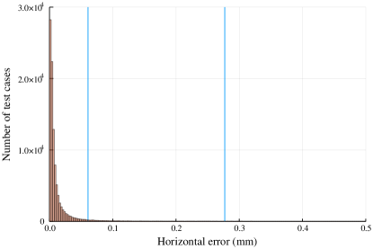
Figure 5: Horizontal positioning errors ($n=5$ emission points) in the Kerr geometry for $10^{5}$ test cases. The vertical lines correspond to the $95\%$ confidence level and rms values for the errors, with respective values of $0.0608$ and $0.277~{}{\rm mm}$. Note that the results here are expressed in units of millimeters. Out of $10^{5}$ samples, four samples ($0.004\%$) have an error $>2~{}{\rm cm}$ with the largest error being $3.39~{}{\rm cm}$.

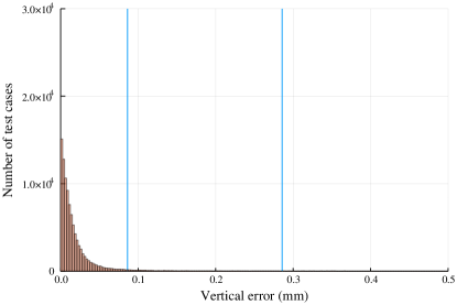
Figure 6: Vertical positioning errors ($n=5$ emission points) in the Kerr geometry for $10^{5}$ test cases. The vertical lines correspond to the $95\%$ confidence level and rms values for the errors, with respective values of $0.0862$ and $0.286~{}{\rm mm}$. Note that the results here are expressed in units of millimeters. Out of $10^{5}$ samples, $1$ sample ($0.001\%$) has an error $>2~{}{\rm cm}$ with the largest error being $2.40~{}{\rm cm}$.

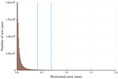
Figure 7: Horizontal positioning errors ($n=5$ emission points) in the analog geometry incorporating tropospheric and ionospheric effects ($10^{5}$ test cases). The vertical lines correspond to the $95\%$ confidence level and rms values for the errors, with respective values of $0.418$ and $0.693~{}{\rm mm}$. Out of $10^{5}$ samples, $13$ samples ($0.013\%$) have an error $>2~{}{\rm cm}$ with the largest error being $3.20~{}{\rm cm}$.

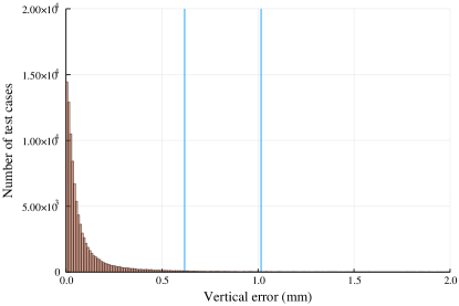
Figure 8: Vertical positioning errors ($n=5$ emission points) in the analog geometry incorporating tropospheric and ionospheric effects ($10^{5}$ test cases). The vertical lines correspond to the $95\%$ confidence level and rms values for the errors, with respective values of $0.618$ and $1.02~{}{\rm mm}$. Out of $10^{5}$ samples, $58$ samples ($0.058\%$) have an error $>2~{}{\rm cm}$ with the largest error being $3.59~{}{\rm cm}$.

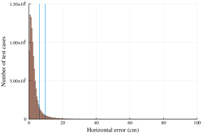
Figure 9: Horizontal positioning errors ($n=5$ emission points) in the perturbed analog geometry corresponding to a fractional uncertainty of $0.1\%$ ($\delta_{1}=10^{-3}$) in the tropospheric index of refraction and $1\%$ ($\delta_{2}=0.01$) in the ionospheric electron density ($10^{5}$ test cases). The vertical lines correspond to the rms and $95\%$ confidence level values for the errors, with respective values of $6.27$ and $9.70~{}{\rm cm}$. Out of $10^{5}$ samples, seven samples ($0.007\%$) have an error $>2~{}{\rm m}$ with the largest error being $3.42~{}{\rm m}$.

Figure 10: Vertical positioning errors ($n=5$ emission points) in the perturbed analog geometry corresponding to a fractional uncertainty of $0.1\%$ ($\delta_{1}=10^{-3}$) in the tropospheric index of refraction and $1\%$ ($\delta_{2}=0.01$) in the ionospheric electron density ($10^{5}$ test cases). The vertical lines correspond to the RMS and $95\%$ confidence level values for the errors, with respective values of $25.6$ and $39.0~{}{\rm cm}$. Out of $10^{5}$ samples, $10$ samples ($0.01\%$) have an error $>2~{}{\rm m}$ with the largest error being $4.56~{}{\rm m}$.

Figure 11: Horizontal positioning errors ($n=5$ emission points) in the perturbed analog geometry corresponding to a fractional uncertainty of $0.1\%$ ($\delta_{1}=10^{-3}$) in the tropospheric index of refraction and $10\%$ ($\delta_{2}=0.1$) in the ionospheric electron density ($10^{5}$ test cases). The vertical lines correspond to the rms and $95\%$ confidence level values for the errors, with respective values of $59.4$ and $93.1~{}{\rm cm}$. Out of $10^{5}$ samples, six samples ($0.006\%$) have an error $>20~{}{\rm m}$ with the largest error being $31.9~{}{\rm m}$.

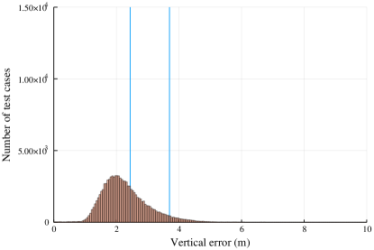
Figure 12: Vertical positioning errors ($n=5$ emission points) in the perturbed analog geometry corresponding to a fractional uncertainty of $0.1\%$ ($\delta_{1}=10^{-3}$) in the tropospheric index of refraction and $10\%$ ($\delta_{2}=0.1$) in the ionospheric electron density ($10^{5}$ test cases). The vertical lines correspond to the rms and $95\%$ confidence level values for the errors, with respective values of $2.44$ and $3.70~{}{\rm m}$. Out of $10^{5}$ samples, $10$ samples ($0.01\%$) have an error $>20~{}{\rm m}$ with the largest error being $42.5~{}{\rm m}$.

VI.2 Test results

Test results for $n=5$ emission points are presented in Figs. 5–12. The vertical errors correspond to errors projected in the direction orthogonal to the WGS-84 reference ellipsoid, and the horizontal errors correspond to errors projected along directions tangent to the WGS-84 ellipsoid. For the Kerr metric, the squirrel.jl code can achieve in most cases submillimeter accuracy, demonstrating a potential for extreme precision in vacuum environments; the methods presented in the squirrel.jl code may be ideal for relativistic location in space navigation. When tropospheric and ionospheric effects are included, the squirrel.jl code yields errors on the order of a centimeter, as illustrated in Figs. 7 and 8.

Figures 9–12 illustrate positioning errors when including uncertainties in the determination of the tropospheric and ionospheric index of refraction. These tests were performed using the perturbation model described in the preceding section; the test cases were generated with the unperturbed metric, and for the tests themselves, the perturbed metric is used in the locator functions of the squirrel.jl code (which take the metric functions as an input). Errors resulting from an uncertainty of $1\%$ in the determination of the ionospheric refractive index are illustrated in Figs. 9 and 10; this is the best result one can realistically expect to achieve with the approximation (51) for GNSS signal frequencies of $\sim 1~{}{\rm GHz}$ (but we reiterate that higher signal frequencies can achieve improved accuracy with the same approximation). Even then, the horizontal positioning errors are for the most part confined to less than $\sim 10~{}{\rm cm}$ to a $95\%$ confidence level, while the vertical errors exhibit a systematic shift of $\sim 20~{}{\rm cm}$, which corresponds to the fact that the perturbations to the index of refraction in our perturbation model are positive, and that the index of refraction profiles vary primarily in the radial direction.

Errors from an uncertainty of $10\%$ in the ionospheric profile are illustrated in Figs. 11 and 12, which increases the horizontal errors to $\sim 1~{}{\rm m}$ and the systematic shift in the vertical errors to $\sim 2~{}{\rm m}$. Upon comparison with the single frequency errors reported in the latest Galileo quarterly report European Union (2021) for the first three months of 2021, we note that the rms and $95\%$ confidence level values are somewhat comparable to the performance of Galileo (rms and $95\%$ C.L. $\sim 1\,{\rm m}$), albeit for a smaller sample size in our case. Of course, the results presented here do not take into account other GNSS errors, such as multipath, satellite timing and ephemeris errors, the latter two of which have been addressed in Puchades Colmenero et al. (2021); Kostić et al. (2015); Gomboc et al. (2014); Čadež et al. (2010); Delva et al. (2011b). In the Galileo error budget, such errors [referred to as signal in space errors (SISE)] are on the order of half a meter European Union (2021), and, for single-frequency users, are smaller in magnitude than the error contributions from ionospheric and tropospheric effects. To compare the errors presented in this article with those of European Union (2021), one should add in quadrature a $\sim 0.5{\rm m}$ contribution from SISE; even with such a correction to the rms and $95\%$ C.L. values presented in Fig. 11 for horizontal positioning, our corrected errors ($0.776~{}{\rm m}~{}[rms]$ and $1.06~{}{\rm m}~{}[95\%C.L.]$) remain smaller than those reported in European Union (2021), and with fewer errors $\geq 20~{}{\rm m}$ in proportion. This indicates a potential for improved performance, even with an uncertainty of $10\%$ in the determination of the ionospheric free electron density and for the stated uncertainties in the determination of atmospheric parameters in the lower troposphere. Moreover, reduced uncertainties in the determination of the ionospheric electron density profile to the $1\%$ level can reduce the $95\%$ C.L. errors by a factor of $10$, to roughly a decimeter.

One can obtain improved accuracy with additional emission points. With $n=6$ emission points, the largest errors are significantly reduced, as indicated in the figures 13– 16 for the cases with $1\%$ and $10\%$ fractional uncertainty in the ionospheric electron density $N_{\rm e}$. These two cases are chosen since they form the boundary cases for the accuracy that one might expect to be achievable with the squirrel.jl code at GNSS signal frequencies of $\sim 1~{}{\rm GHz}$. In both cases, we find a significant reduction in the number of large errors for $n=6$ emission points. There were no errors above the stated thresholds for the $n=5$ cases ($2~{}{\rm m}$ for the $1\%$ case and $20~{}{\rm m}$ for the $10\%$ case); for the $n=6$ cases, we find only one sample with an error $>1~{}{\rm m}$ threshold for a $1\%$ uncertainty in $N_{\rm e}$, and seven samples with horizontal errors $>5~{}{\rm m}$ a $10\%$ uncertainty in $N_{\rm e}$. The rms and $95\%$ confidence level errors are roughly the same for the vertical errors (owing to the systematic shift that the perturbations introduce), but are reduced by a factor of $2$ for the horizontal errors. This result indicates that, in principle, the inclusion of additional emission points can significantly reduce the number of large errors in the squirrel.jl code.

Figure 13: Horizontal positioning errors ($n=6$ emission points) in the perturbed analog geometry corresponding to a fractional uncertainty of $0.1\%$ ($\delta_{1}=10^{-3}$) in the tropospheric index of refraction and $1\%$ ($\delta_{2}=0.01$) in the ionospheric electron density ($10^{5}$ test cases). The vertical lines correspond to the rms and $95\%$ confidence level values for the errors, with respective values of $3.27$ and $5.81~{}{\rm cm}$. Out of $10^{5}$ samples, $1$ sample ($0.001\%$) has an error $>1~{}{\rm m}$ (none greater than $2~{}{\rm m}$) with the largest error being $1.56~{}{\rm m}$.

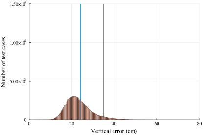
Figure 14: Vertical positioning errors ($n=6$ emission points) in the perturbed analog geometry corresponding to a fractional uncertainty of $0.1\%$ ($\delta_{1}=10^{-3}$) in the tropospheric index of refraction and $1\%$ ($\delta_{2}=0.01$) in the ionospheric electron density ($10^{5}$ test cases). The vertical lines correspond to the rms and $95\%$ confidence level values for the errors, with respective values of $24.2$ and $35.0~{}{\rm cm}$. Out of $10^{5}$ samples, $1$ sample ($0.001\%$) have an error $>1~{}{\rm m}$ (none greater than $2~{}{\rm m}$) with the largest error being $1.10~{}{\rm m}$.

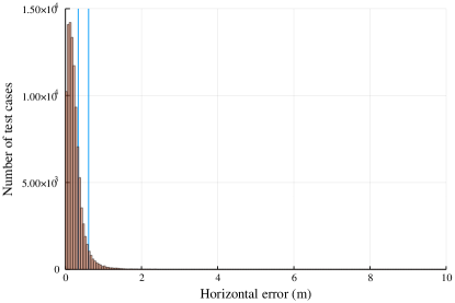
Figure 15: Horizontal positioning errors ($n=6$ emission points) in the perturbed analog geometry corresponding to a fractional uncertainty of $0.1\%$ ($\delta_{1}=10^{-3}$) in the tropospheric index of refraction and $10\%$ ($\delta_{2}=0.1$) in the ionospheric electron density ($10^{5}$ test cases). The vertical lines correspond to the rms and $95\%$ confidence level values for the errors, with respective values of $33.5$ and $61.1~{}{\rm cm}$. Out of $10^{5}$ samples, seven samples ($0.007\%$) samples have an error $>5~{}{\rm m}$ with the largest error being $14.6~{}{\rm m}$.

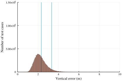
Figure 16: Vertical positioning errors ($n=6$ emission points) in the perturbed analog geometry corresponding to a fractional uncertainty of $0.1\%$ ($\delta_{1}=10^{-3}$) in the tropospheric index of refraction and $10\%$ ($\delta_{2}=0.1$) in the ionospheric electron density ($10^{5}$ test cases). The vertical lines correspond to the rms and $95\%$ confidence level values for the errors, with respective values of $2.32$ and $3.24~{}{\rm m}$. Out of $10^{5}$ samples, five samples ($0.005\%$) samples have an error $>7~{}{\rm m}$ with the largest error being $10.4~{}{\rm m}$.

VI.3 Benchmarks

Execution time for squirrel.jl
$N$	Kerr-Schild	Gordon	Pert. Gordon
4	27 ms	193 ms	223 ms
5	101 ms	553 ms	588 ms
6	358 ms	1.74 s	1.95 s

Table 1: Benchmarks performed with squirrel.jl. $N$ is the number of emission points. Tests were performed with the Kerr-Schild metric, the unperturbed Gordon metric, and the perturbed Gordon metric corresponding to a $10\%$ uncertainty in the ionospheric profile.

Some basic benchmarks have been performed for various situations; the results are displayed in Table 1. The results we report were obtained on standard desktop computer with an Intel i5-7500 processor, and with four threads enabled. The benchmarks were performed for three geometries: the Kerr-Schild metric, the unperturbed Gordon metric (representing tropospheric and ionospheric effects), and the perturbed Gordon metric corresponding to a $10\%$ uncertainty in the ionospheric profile. We consider three cases, with $N=4,5,6$ emission points. We note that the $N=4$ Kerr-Schild case has an execution time comparable to that reported in Gomboc et al. (2014); Kostić et al. (2015) for a Schwarzschild location method. In the case of $N=4$ emission points, the flat spacetime methods of Coll et al. (2010b, 2012) and Sec. II.2 return two guesses due to the bifurcation problem, so the squirrel algorithm is applied twice (one for each guess) for $N=4$ emission points. This is seen in the fact that the execution time for $N=4$ is longer than one might expect from the number of combinations $C(5,4)=5$, which is supported by the execution times for the Gordon and perturbed Gordon cases. Comparing the $N=5$ and $N=6$ cases, we find a scaling roughly consistent with the number of combinations $C(5,4)=5$, $C(6,4)=15$, which suggests an increase in computational complexity by a factor of $3$.

VII Summary and discussion

In this article, we have described and demonstrated a new method for relativistic location in slightly curved, but otherwise generic spacetime geometries. Though such methods may be of primary interest for high precision space navigation in regions beyond the ionosphere, we have demonstrated, by way of simple analog gravity models, that our method can nonetheless be used to incorporate tropospheric and ionospheric effects in terrestrial positioning. Though one might regard such effects as ancillary from a purely general relativistic perspective, we argue that they are still of fundamental importance in the sense that the placement of emission coordinates near the surface of the Earth will depend on the knowledge of the profile for the effective tropospheric and ionospheric refractive index.

The methods we have described and implemented FHC make use of state of the art automatic differentiation and ODE libraries available in the Julia language, which permit the efficient evaluation of the derivatives of numerical solutions of the geodesic equation performed with respect to initial data. Combined with a quasi-Newton root-finding algorithm, we have demonstrated that our methods can, with guesses provided by the flat spacetime relativistic location formula of Ruggiero et al. (2022), accurately and efficiently compute the intersection point of future pointing null cones from a set of spacelike separated emission points. In particular, our implementation, the squirrel.jl code Feng et al. (2022b), can with five emission points achieve submillimeter accuracy for terrestrial positioning (satellite orbits at $\sim 26.5\times 10^{3}~{}{\rm km}$, target point at surface of Earth) in a vacuum Kerr-Schild metric. When tropospheric and ionospheric effects are included by way of the Gordon metric, the squirrel.jl code can achieve horizontal errors of less than $\sim 1~{}{\rm m}$ (according to rms and $95\%$ C.L. values for $10^{5}$ samples) for a $10\%$ uncertainty in the ionospheric free electron density profile, and to less than $\sim 10~{}{\rm cm}$ for a $1\%$ uncertainty, with an execution time of $<1~{}{\rm s}$ on a desktop computer for five emission points. An interesting question for future investigation is whether multifrequency methods may be used in conjunction with our algorithm to constrain the electron density profile.

Our test results indicate that the relativistic location algorithm implemented in the squirrel.jl code can achieve extreme precision for space navigation in vacuum regions beyond the ionosphere; we will describe in detail the applications of our methods to deep space navigation elsewhere. Our tests also indicate that implementations of our method have the potential for performance comparable to or exceeding the single-frequency performance of Galileo, assuming that the local atmospheric properties of the troposphere are known to typical measurement uncertainties and the ionospheric free electron profile is known to an uncertainty of $10\%$ or less. Alternatively, the methods presented in this article may perhaps be of interest as an additional method for atmospheric tomography (see Jin et al. (2014) and references therein for an overview of methods in GNSS tomography).

The results we have presented here are complementary to those of Puchades Colmenero et al. (2021); Kostić et al. (2015); Gomboc et al. (2014); Čadež et al. (2010); Delva et al. (2011b), which address the problem of incorporating general relativistic effects in the determination of satellite ephemerides; satellite ephemeris and timing errors (SISE) are some the largest contributors to GNSS error budgets. A more comprehensive collection of methods for relativistic positioning will require at the minimum a relativistic location algorithm and an algorithm for determining satellite ephemerides and for mitigating clock errors. These issues can in principle be addressed in a more general optimization framework based on emission coordinates, as discussed in Tarantola et al. (2009); the implementation of this framework using modern machine learning methods will be explored in future work.