Understanding Entropy Coding With Asymmetric Numeral Systems (ANS): a Statistician’s Perspective

Abstract

Entropy coding is the backbone data compression. Novel machine-learning based compression methods often use a new entropy coder called Asymmetric Numeral Systems (ANS) [Duda et al., 2015], which provides very close to optimal bitrates and simplifies [Townsend et al., 2019] advanced compression techniques such as bits-back coding. However, researchers with a background in machine learning often struggle to understand how ANS works, which prevents them from exploiting its full versatility. This paper is meant as an educational resource to make ANS more approachable by presenting it from a new perspective of latent variable models and the so-called bits-back trick. We guide the reader step by step to a complete implementation of ANS in the Python programming language, which we then generalize for more advanced use cases. We also present and empirically evaluate an open-source library of various entropy coders designed for both research and production use. Related teaching videos and problem sets are available online.

1 Introduction

Effective data compression is becoming increasingly important. Digitization in business and science raises the demand for data storage, and the proliferation of remote working arrangements makes high-quality videoconferencing indispensable. Recently, novel compression methods that employ probabilistic machine-learning models have been shown to outperform more traditional compression methods for images and videos [Ballé et al., 2018, Minnen et al., 2018, Yang et al., 2020a, Agustsson et al., 2020, Yang et al., 2021]. Machine learning provides new methods for the declarative task of expressing complex probabilistic models, which are essential for data compression (see Section 2.1). However, many researchers who come to data compression from a machine learning background struggle to understand the more procedural (i.e., algorithmic) parts of a compression pipeline.

This paper discusses an integral algorithmic part of lossless and lossy data compression called entropy coding. We focus on the Asymmetric Numeral Systems (ANS) entropy coder [Duda et al., 2015], which is the method of choice in many recent proposals of machine-learning based compression methods [Townsend et al., 2019, Kingma et al., 2019, Yang et al., 2020a, Theis and Ho, 2021]. We intend to make the internals of ANS more approachable to statisticians and machine learning researchers by presenting them from a new perspective based on latent variable models and the so-called bits-back trick [Wallace, 1990, Hinton and Van Camp, 1993], which we explain below. We show that this new perspective allows us to come up with novel variants of ANS that enable research on new compression methods which combine declarative with procedural tasks.

This paper is written in an educational style that favors real code examples over pseudocode, culminating in a working demo implementation of ANS in the Python programming language (Listing 3.3 on page 3.3). The paper is structured as follows: Section 2 reviews the relevant information theory and introduces the concept of stream codes. Section 3 presents our statistical perspective on the ANS algorithm and guides the reader to a full implementation. In Section 4, we show that understanding the internals of ANS allows us to create new variations on it for special use cases. Section 5 presents and empirically evaluates an open-source compression library that is more run-time efficient and easier to use than our demo implementation in Python. We provide concluding remarks in Section 6.

2 Background

In Subsection 2.1, we briefly review the relevant theory of lossless compression. In Subsection 2.2, we summarize how the Asymmetric Numeral Systems (ANS) method differs from other stream codes (like Arithmetic Coding or Range Coding) and from symbol codes (like Huffman Coding).

2.1 Fundamentals of Lossless Compression

We formalize the problem of lossless compression and state the theoretical bounds from the source coding theorem. Readers who are already familiar with source coding may opt to skip this section.

Problem Statement.

A lossless compression algorithm (or “code”) $C$ maps any message ${{\mathbf{x}}}$ from some discrete messages space ${\boldsymbol{\mathcal{X}}}$ to a bit string $C({{\mathbf{x}}})$. We want to make these bit strings $C({{\mathbf{x}}})$ as short as possible while still keeping the mapping $C$ injective, so that a decoder can reconstruct the message ${{\mathbf{x}}}$ by inverting $C$. We refer to the length of the bit string $C({{\mathbf{x}}})$ as the bitrate $R_{C}({{\mathbf{x}}})$. Since $R_{C}({{\mathbf{x}}})$ may depend on ${{\mathbf{x}}}$, a common (albeit not the only reasonable) goal in the lossless compression literature is to find a code $C$ that minimizes the expected bitrate ${\mathbb{E}}_{P}[R_{C}({{\mathbf{X}}})]$. Here, $P$ is a probability distribution over ${\boldsymbol{\mathcal{X}}}$, i.e., a probabilistic model of the data source (called the “entropy model” for short). Further, ${\mathbb{E}}_{P}[\,\cdot\,]$ is the expectation value, and capital letters like ${{\mathbf{X}}}$ denote random variables.

To minimize ${\mathbb{E}}_{P}[R_{C}({{\mathbf{X}}})]$, a code $C$ exploits knowledge of $P$ to map probable messages to short bit strings while mapping less probable messages to longer bit strings (to avoid clashes that would make $C$ non-injective). Thus, the bitrate $R_{C}({{\mathbf{x}}})$ varies across messages ${{\mathbf{x}}}\in{\boldsymbol{\mathcal{X}}}$. In order to prevent $C$ from encoding information about ${{\mathbf{x}}}$ into the length rather than the contents of $C({{\mathbf{x}}})$, we will assume in the following that $C$ is uniquely decodable. This means that it must be possible to reconstruct a sequence of messages from the (delimiter-free) concatenation of their compressed representations.

Theoretical Bounds.

The source coding theorem [Shannon, 1948] makes two fundamental statements—a negative and a positive one—about the expected bitrate, relating it to the entropy $H_{P}[{{\mathbf{X}}}]:={\mathbb{E}}_{P}[-\log_{2}P({{\mathbf{X}}})]$ of the message ${{\mathbf{X}}}$ under the entropy model $P$. The negative part of the theorem states that the expected bitrate of any uniquely decodable lossless code cannot be smaller than the entropy of the message. The positive part states that, if we allow for up to one bit of overhead over the entropy, then there indeed always exists a uniquely decodable lossless code. More formally,

$$\forall P \forall C {\mathbb{E}}_{P}[R_{C}({{\mathbf{X}}})]\geq H_{P}[{{\mathbf{X}}}];\;\text{and}$$ entropy models , uniquely decodable lossless codes : (1)

$$\forall P \exists C {\mathbb{E}}_{P}[R_{C}({{\mathbf{X}}})]<H_{P}[{{\mathbf{X}}}]+1.$$ entropy models , uniquely decodable lossless code : (2)

Thus, the expected bitrate of an optimal code $C_{P}^{*}$ lies in the half-open interval $[H_{P}[{{\mathbf{X}}}],H_{P}[{{\mathbf{X}}}]+1)$. A so-called entropy coder takes an entropy model $P$ as input and constructs a near-optimal code for it. The model $P$ and the choice of entropy coder together comprise a compression method on which two parties have to agree before they can meaningfully exchange any compressed data.

Information Content.

The upper bound in Eq. 2 is actually a corollary of a more powerful statement. Recall that the entropy $H_{P}[{{\mathbf{X}}}]={\mathbb{E}}_{P}[-\log_{2}P({{\mathbf{X}}})]$ is an expectation over the quantity “$-\log_{2}P({{\mathbf{X}}})$”. This quantity is called the information content of ${{\mathbf{X}}}$. Eq. 2 thus relates two expectations under $P$, and it turns out that there exists a code (the so-called Shannon Code [Shannon, 1948]) where the inequality holds not only in expectation but indeed for all messages individually, i.e.,

$$\!\!\text{$\forall$ entropy models~{}$P$, $\exists$ uniqly.~{}dec.~{}lossless code~{}$C$: $\forall{{\mathbf{x}}}\!\in\!{\boldsymbol{\mathcal{X}}}\!:\,R_{C}({{\mathbf{x}}})<-\log_{2}P({{\mathbf{X}}}\!=\!{{\mathbf{x}}})+1$}.$$ (3)

For large message spaces (e.g., the space of all conceivable HD images), $P({{\mathbf{X}}}\!=\!{{\mathbf{x}}})$ is usually very small for any particular ${{\mathbf{x}}}$, and the “$+1$” on the right-hand side of Eq. 3 is negligible compared to the information content $-\log_{2}P({{\mathbf{X}}}\!=\!{{\mathbf{x}}})$. In this regime, the information content of a message ${{\mathbf{x}}}$ is thus a very accurate estimate of its bitrate $R_{C_{P}^{*}}({{\mathbf{x}}})$ under a (hypothetical) optimal code $C_{P}^{*}$.

Trivial Example: Uniform Entropy Model.

To obtain some intuition for Eqs. 1-3, we briefly consider a trivial case, from which our discussion of ANS in Section 3 below will start. Consider a finite message space ${\boldsymbol{\mathcal{X}}}$ with a uniform entropy model $P$, i.e., ${P({{\mathbf{X}}}\!=\!{{\mathbf{x}}})}={1}/{|{\boldsymbol{\mathcal{X}}}|}\;\forall{{\mathbf{x}}}\!\in\!{\boldsymbol{\mathcal{X}}}$. Thus, each message ${{\mathbf{x}}}\in{\boldsymbol{\mathcal{X}}}$ has information content $-\log_{2}{P({{\mathbf{X}}}\!=\!{{\mathbf{x}}})}={\log_{2}|{\boldsymbol{\mathcal{X}}}|}$, and we have $H_{P}[{{\mathbf{X}}}]=\log_{2}|{\boldsymbol{\mathcal{X}}}|$. We can trivially find a uniquely decodable code $C_{\text{unif.}}$ that satisfies Eqs. 2-3 for this model $P$: we simply enumerate all ${{\mathbf{x}}}\in{\boldsymbol{\mathcal{X}}}$ with integer labels from $\{0,\ldots,|{\boldsymbol{\mathcal{X}}}|-1\}$, which we then express in binary. The binary representation of the largest label $(|{\boldsymbol{\mathcal{X}}}|-1)$ works out to be $\lceil\log_{2}|{\boldsymbol{\mathcal{X}}}|\rceil$ bits long where $\lceil\cdot\rceil$ denotes rounding up to the nearest integer. To ensure unique decodability, we pad shorter bit strings to the same length with leading zeros. Thus, $R_{C_{\text{unif.}}}({{\mathbf{x}}})=\left\lceil\log_{2}|{\boldsymbol{\mathcal{X}}}|\right\rceil=\left\lceil-\log_{2}P({{\mathbf{X}}}\!=\!{{\mathbf{x}}})\right\rceil$ for all ${{\mathbf{x}}}\in{\boldsymbol{\mathcal{X}}}$, which satisfies Eq. 3 and therefore also Eq. 2. According to Eq. 1, this trivial code $C_{\text{unif.}}$ has less than one bit of overhead over the optimal code for such a uniform entropy model.

In practice, however, the entropy model $P$ is rarely a uniform distribution. For example, in a compression method for natural language, $P$ should assign higher probability to this paragraph than to some random gibberish. Any such non-uniform $P$ has entropy $H_{P}[{{\mathbf{X}}}]<\log_{2}|{\boldsymbol{\mathcal{X}}}|$ and thus, according to Eq. 2, there exists a better code for $P$ than the trivial $C_{\text{unif.}}$. In principle, one could find an optimal code for any entropy model $P$ (over a finite ${\boldsymbol{\mathcal{X}}}$) via the famous Huffman algorithm [Huffman, 1952] (knowledge of this algorithm is not required to understand the present paper). However, directly applying the Huffman algorithm to entire messages would usually be prohibitively computationally expensive. The next section provides an overview of computationally feasible alternatives.

2.2 Symbol Codes vs. Stream Codes

Practical lossless entropy coding methods trade off some compression performance for better runtime and memory efficiency. There are two common approaches: symbol codes and stream codes [MacKay and Mac Kay, 2003]. Both assume that a message ${{\mathbf{x}}}\equiv(x_{1},\ldots,x_{k})$ is a sequence (with length $k$) of symbols $x_{i}\in{\mathfrak{X}}\;\forall i\in\{1,\ldots,k\}$, with some discrete set (“alphabet”) ${\mathfrak{X}}$. Further, both approaches assume that the entropy model $P({{\mathbf{X}}})=\prod_{i=1}^{k}P_{i}(X_{i})$ is a product of per-symbol entropy models $P_{i}$. Thus, the entropy of the message ${{\mathbf{X}}}$ is the sum of all symbol entropies: $H_{P}[{{\mathbf{X}}}]=\sum_{i=1}^{k}H_{P_{i}}[X_{i}]$.

Constructing an optimal code over the message space ${\boldsymbol{\mathcal{X}}}={\mathfrak{X}}^{k}$ by Huffman coding would require $O(|{\mathfrak{X}}|^{k})$ runtime (and memory) since Huffman coding builds a tree over all ${{\mathbf{x}}}\in{\boldsymbol{\mathcal{X}}}$. Both symbol and stream codes reduce the runtime complexity to $O(k)$, but they differ in their precise practical run-time cost and, more fundamentally, in their overhead over the minimal expected bitrate (Eq. 1).

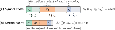
Figure 1: Comparison between (a) symbol codes (here: Shannon Coding) and (b) stream codes (here: Arithmetic Coding). Symbol codes assign an integer number of bits to each symbol $x_{i}$, which leads to a significant overhead in bitrate if the information content per symbol ($-\log_{2}P(X_{i}\!=\!x_{i})$) is low.

Symbol Codes.

Symbol codes are illustrated in Figure 1 (a). They simply apply a uniquely decodable code (e.g., a Huffman code) independently to each symbol $x_{i}$ of the message, and then concatenate the resulting bit strings. This makes the runtime linear in $k$ but it increases the bitrate. Even if we use an optimal code $C_{P_{i}}^{*}$ for each symbol $x_{i}$, the expected bitrate of each symbol can exceed the symbol’s entropy $H_{P_{i}}[X_{i}]$ by up to one bit (see Eq. 2). Since this overhead now applies per symbol, the overhead in expected bitrate for the entire message now grows linearly in $k$.

Symbol codes are used in many classical compression methods such as gzip [Deutsch, 1996] and png [Boutell and Lane, 1997]. Here, the entropy per symbol is large enough that an overhead of up to one bit per symbol can be tolerated. By contrast, recently proposed machine-learning based compression methods [Ballé et al., 2017, 2018, Yang et al., 2020b, a] often spread the total entropy of the message over a larger number $k$ of symbols, resulting in much lower entropy per symbol. For example, with about $0.3$ bits of entropy per symbol, a symbol code (which needs at least one full bit per symbol) would have an overhead of more than $200\%$, thus rendering the method useless.

Stream Codes.

Stream codes reduce the overhead of symbol codes without sacrificing computational efficiency by amortizing over symbols. Similar to symbol codes, stream codes also encode and decode one symbol at a time, and their runtime cost is linear in the message length $k$. However, stream codes do not directly map each individual symbol to a bit string. Instead, for most encoded symbols, a stream code does not immediately emit any compressed bits but instead merely updates some internal encoder state that accumulates information. Only every once in a while (when the internal state overflows), does the encoder emit some compressed bits that “pack” the information content of several symbols more tightly together than in a symbol code (see illustration in Figure 1 (b)).

The most well-known stream codes are Arithmetic Coding (AC) [Rissanen and Langdon, 1979, Pasco, 1976] and its more efficient variant Range Coding (RC) [Martin, 1979]. This paper focuses on a more recently proposed (and currently less known) stream code called Asymmetric Numeral Systems (ANS) [Duda et al., 2015]. In practice, all three of these stream codes usually have negligible overhead over the fundamental lower bound in Eq. 1 (see Section 5.2 for empirical results). From a user’s point of view, the main difference between these stream codes is that AC and RC operate as a queue (“first in first out”, i.e., symbols are decoded in the same order in which they were encoded) while ANS operates as a stack (“last in first out”). A queue simplifies compression with autoregressive models while a stack simplifies compression with latent variable models and is generally the simpler data structure for more involved use cases (since reads and writes happen only at a single position).

Further, ANS provides some more subtle advantages over AC and RC:

• ANS is better suited than AC and RC for advanced compression techniques such as bits-back coding [Wallace, 1990, Hinton and Van Camp, 1993] because (i) AC and RC treat encoding and decoding asymmetrically with different internal coder states that satisfy different invariants, which complicates switching between encoding and decoding; and (ii) while encoding with RC is, of course, injective, it is difficult to make it surjective (and thus to make decoding arbitrary bit strings injective). ANS has neither of these two issues.

• While the main idea of AC and RC is simple, details are somewhat involved due to a number of edge cases. By contrast, a complete ANS coder can be implemented in just a few lines of code (see Listing 3.3 in Section 3.3 below). Further, this paper provides a new perspective on ANS that conceptually splits the algorithm into three parts. Combining these parts in new ways allows us to design new variants of ANS for special use cases (see Section 4.3).

• As a minor point, decoding with AC and RC is somewhat slow because it updates an internal state that is larger than that of the encoder, and because it involves integer division (which is slow on standard hardware [Fog, 2021]). By contrast, decoding with ANS is a very simple operation (assuming that evaluating the model $P_{i}$ is cheap, as in a small lookup table).

We present the basic ANS algorithm in Section 3, discuss possible extensions to it in Section 4, and empirically compare its compression performance and runtime efficiency to AC and RC in Section 5.

3 From Positional Numeral Systems to Asymmetric Numeral Systems

This section guides the reader towards a full implementation of an Asymmetric Numeral Systems (ANS) entropy coder. We start with a trivial coder for sequences of uniformly distributed symbols (Subsection 3.1), generalize it to arbitrary entropy models (Subsection 3.2), and finally make it computationally efficient (Subsection 3.3). Our presentation of ANS differs from the original proposal [Duda et al., 2015] in that it builds on latent variable models and the so-called bits-back trick, which we hope makes it more approachable to statisticians and machine learning researchers.

3.1 A Simple Stream Code: Positional Numeral Systems

We introduce our first example of a stream code: a simple code that provides optimal compression performance for sequences of uniformly distributed symbols. This code will serve as a fundamental building block in our implementation of Asymmetric Numeral Systems in Sections 3.2-3.3 below.

As shown in Section 2.1, we can obtain an optimal lossless compression code $C_{\text{unif.}}$ for a uniform entropy model over a finite message space ${\boldsymbol{\mathcal{X}}}$ by using a bijective mapping from ${\boldsymbol{\mathcal{X}}}$ to $\{0,\ldots,|{\boldsymbol{\mathcal{X}}}|-1\}$ and expressing the resulting integer in binary. Such a bijective mapping can be done efficiently if messages are sequences $(x_{1},\ldots,x_{k})$ of symbols $x_{i}\in{\mathfrak{X}}$ from a finite alphabet ${\mathfrak{X}}$: we simply interpret the symbols as the digits of a number in the positional numeral system of base $|{\mathfrak{X}}|$. For example, if the alphabet size is $|{\mathfrak{X}}|=10$ then we can assume, without loss of generality, that ${\mathfrak{X}}=\{0,1,\ldots,9\}$. To encode, e.g., the message ${{\mathbf{x}}}=(3,6,5)$ we thus simply parse it as the decimal number $365$, which we then express in binary: $365={(101101101)}_{2}$. We defer the issue of unique decodability to Section 3.3. Despite its simplicity, this code has three important properties, which we highlight next.

Property 1: “Stack” Semantics.

Encoding and decoding traverse symbols in a message in opposite order. For encoding, the simplest way to parse a sequence of digits $x_{i}\in{\mathfrak{X}}$ into a number in the positional numeral system of base $|{\mathfrak{X}}|$ goes as follows: initialize a variable with zero; then, for each digit, multiply the variable with $|{\mathfrak{X}}|$ and add the digit. For example, if $|{\mathfrak{X}}|=10$ and ${{\mathbf{x}}}=(3,6,5)$:

Parsing the decimal number $365$:

Encoding thus reads the digits of the decimal number $365$ from left to right, i.e., from most to least significant digit. By contrast, decoding the number back into its digits is easier done in reverse order: keep dividing the number by the base $|{\mathfrak{X}}|$, rounding down and recording the remainders as the digits:

Generating the digits of the decimal number $365$:

⬇

class UniformCoder: # optimal code for uniformly distributed symbols

def __init__(self, number=0): # constructor with an optional argument

self.number = number

\pardef push(self, symbol, base): # Encodes a @$\mathtt{symbol} \in\{0, \ldots, \mathtt{base}-1\}$@.

self.number = self.number * base + symbol

\pardef pop(self, base): # Decodes a @$\mathtt{symbol} \in\{0, \ldots, \mathtt{base}-1\}$@.

symbol = self.number self.number //= base # “@{\normalfont\texttt{//}}@” denotes integer division.

return symbol

Figure 2: Python implementation of a stack-based optimal encoder/decoder for sequences of uniformly distributed symbols, as discussed in Section 3.1; for usage examples, see Listings 3 and 4.

⬇

coder = UniformCoder() # Defined in Listing |\ref*{listing:pns}|.

\par# Encode the message |$\vx=(3,6,5)$|:

coder.push(3, base=10) # |{\normalfont\texttt{base=10}}| means that the alphabet is |$\XX=\{0, \ldots, 9\}$|.

coder.push(6, base=10)

coder.push(5, base=10)

print(f"Encoded number: {coder.number}") # Prints: “Encoded number: 365”

print(f"In binary: {coder.number:b}") # Prints: “In binary: 101101101”

\par# Decode the encoded symbols (in reverse order):

print(f"Decoded ’{coder.pop(base=10)}’.") # Prints: “Decoded ’5’.”

print(f"Decoded ’{coder.pop(base=10)}’.") # Prints: “Decoded ’6’.”

print(f"Decoded ’{coder.pop(base=10)}’.") # Prints: “Decoded ’3’.”

Figure 3: Encoding and decoding the message ${{\mathbf{x}}}=(3,6,5)$ using our UniformCoder from Listing 2; digits are encoded from left to right but decoded from right to left, i.e., the coder has stack semantics.

Thus, the simplest implementation of $C_{\text{unif.}}$ has “stack” semantics (last-in-first-out): conceptually, encoding pushes information onto the top of a stack of compressed data, and decoding pops the latest encoded information off the top of the stack. Listing 2 implements these push and pop operations in Python as methods on a class UniformCoder. A simple usage example is given in Listing 3 (all code examples in this paper are also available online as an executable jupyter notebook.)

Property 2: Amortization.

Before we explore more advanced usages of our UniformCoder from Listing 2, we illustrate how this stream code amortizes compressed bits over multiple symbols (see Section 2.2). Consider again encoding the message ${{\mathbf{x}}}=(3,6,5)$ with the alphabet ${\mathfrak{X}}=\{0,\ldots,9\}$. Modifying one of the symbols in this message obviously changes the compressed bit string, e.g.,

$$\begin{array}[]{r@{$\;=\;$}c@{$\;\!$}c@{$\;\!$}c@{$\;\!$}c@{$\;\!$}c@{$\;\!$}c@{$\;\!$}c@{$\;\!$}c@{$\;\!$}c@{$\;\!$}l}C_{\text{unif.}}\big{(}(3,6,5)\big{)}&1&0&1&1&0&1&1&{\color[rgb]{0.7,0,0}0}&1&;\\[3.0pt] C_{\text{unif.}}\big{(}(3,6,\underline{6})\big{)}&1&0&1&1&0&1&1&\underline{\color[rgb]{0.7,0,0}1}&\underline{0}&;\\[3.0pt] C_{\text{unif.}}\big{(}(3,\underline{7},5)\big{)}&1&0&1&1&\underline{1}&\underline{0}&1&\underline{\color[rgb]{0.7,0,0}1}&1&.\end{array}$$ (7)

Here, underlined numbers highlight differences to $C_{\text{unif.}}\big{(}(3,6,5)\big{)}$ (first line). Note that the penultimate bit (red) changes from “0” to “1” when we change the third symbol from $x_{3}=5$ to $x_{3}=6$ (second line), and also when we change the second symbol from $x_{2}=6$ to $x_{2}=7$ (third line). Thus, this bit depends on both $x_{2}$ and $x_{3}$. This is a crucial difference to symbol codes (e.g., Huffman Codes), which attribute each bit in the compressed bit string to exactly one symbol only (see Figure 1 (a)). Amortization is what allows stream codes to reach lower expected bitrates than symbol codes.

⬇

coder = UniformCoder() # Defined in Listing |\ref*{listing:pns}|.

\par# Encode a sequence of symbols from alphabets of varying sizes:

coder.push( 3, base=10) # |{\normalfont\texttt{base=10}}| means that the alphabet is |$\{0, \ldots, 9\}$|.

coder.push( 6, base=10)

coder.push(12, base=15) # Setting |{\normalfont\texttt{base=15}}| switches to alphabet |$\{0, \ldots, 14\}$|.

coder.push( 4, base=15)

print(f"Binary: {coder.number:b}") # Prints: “Binary: 10000001011100”

\par# For decoding, use the same sequence of bases but in *reverse* order:

print(f"Decoded ’{coder.pop(base=15)}’.") # Prints: “Decoded ’4’.”

print(f"Decoded ’{coder.pop(base=15)}’.") # Prints: “Decoded ’12’.”

print(f"Decoded ’{coder.pop(base=10)}’.") # Prints: “Decoded ’6’.”

print(f"Decoded ’{coder.pop(base=10)}’.") # Prints: “Decoded ’3’.”

Figure 4: Encoding and decoding the message ${{\mathbf{x}}}=(3,6,12,4)$ where the first two symbols come from the alphabet $\{0,\ldots,9\}$ and the last two symbols come from the alphabet $\{0,\ldots,14\}$.

Property 3: Varying Alphabet Sizes.

Our implementation of ANS in Sections 3.2-3.3 below will exploit an additional property of the UniformCoder from Listing 2: each symbol $x_{i}$ of the message ${{\mathbf{x}}}=(x_{1},\ldots,x_{k})$ may come from an individual alphabet ${\mathfrak{X}}_{i}$, with individual alphabet size $|{\mathfrak{X}}_{i}|$. We just have to set the base when encoding or decoding each symbol $x_{i}$ to the corresponding alphabet size $|{\mathfrak{X}}_{i}|$. For example, in Listing 4 we encode and decode the example message ${{\mathbf{x}}}\!=\!(3,6,12,4)$ using the alphabet ${\mathfrak{X}}_{1}\!=\!{\mathfrak{X}}_{2}\!=\!\{0,\ldots,9\}$ for the first two symbols and the alphabet ${\mathfrak{X}}_{3}\!=\!{\mathfrak{X}}_{4}\!=\!\{0,\ldots,14\}$ for the last two symbols. The example works because the method pop of UniformCoder (Listing 2) performs the exact inverse of push: calling push(symbol, base) followed by pop(base) with identical base (and with $\texttt{symbol}\in\{0,\ldots,\texttt{base}-1\}$) restores the coder’s internal state, regardless of its history. This generalized use of a UniformCoder still maps bijectively between the message space (which is now ${\boldsymbol{\mathcal{X}}}={\mathfrak{X}}_{1}\times{\mathfrak{X}}_{2}\times\ldots\times{\mathfrak{X}}_{k}$) and the integers $\{0,\ldots,|{\boldsymbol{\mathcal{X}}}|-1\}$. It therefore still provides optimal compression performance assuming that all symbols are uniformly distributed over their respective alphabets. In the next section, we lift this restriction on uniform entropy models.

3.2 Latent Variable Models and the Bits-Back Trick

In this section, we use the UniformCoder introduced in the last section (Listing 2) as a building block for a more general stream code that is no longer limited to uniform entropy models. This leads us to a precursor of ANS that provides very close to optimal compression performance for arbitrary entropy models, but that is too slow for practical use. We will speed it up in Section 3.3 below.

Approximated Entropy Model.

The UniformCoder from Listing 2 minimizes the expected bitrate ${\mathbb{E}}_{P}[R_{C_{\text{unif.}}}({{\mathbf{X}}})]$ only if the entropy model $P$ is a uniform distribution. We now consider the more general case where $P({{\mathbf{X}}})=\prod_{i=1}^{k}P_{i}(X_{i})$ still factorizes over all symbols, but each $P_{i}$ is now an arbitrary distribution over a finite alphabet ${\mathfrak{X}}_{i}$. The ANS algorithm approximates each $P_{i}$ with a distribution $Q_{i}$ that represents the probability $Q_{i}(X_{i}\!=\!x_{i})$ of each symbol $x_{i}$ in fixed point precision,

$$Q_{i}(X_{i}\!=\!x_{i})=\frac{m_{i}(x_{i})}{n}\quad\forall x_{i}\in{\mathfrak{X}}_{i},\qquad\text{where $n=2^{\mathtt{precision}}$.}$$ (8)

Here, $\mathtt{precision}$ is a positive integer (typically $\lesssim 32$) that controls a trade-off between computational cost and accuracy of the approximation. Further, $m_{i}(x_{i})$ for ${x_{i}\in{\mathfrak{X}}_{i}}$ are integers that should ideally be chosen by minimizing the Kullback-Leibler (KL) divergence $D_{\text{KL}}(P_{i}\,||\,Q_{i})$, which measures the overhead (in expected bitrate) due to approximation errors. In practice, however, exact minimization of this KL-divergence is rarely necessary as simpler heuristics (e.g., by lazily rounding the cumulative distribution function) usually already lead to a negligible overhead for reasonable precisions. Note however, that setting $m_{i}(x_{i})=0$ for any ${x_{i}\in{\mathfrak{X}}_{i}}$ makes it impossible to encode $x_{i}$ with ANS, and that correctness of the ANS algorithm relies on $Q_{i}$ being properly normalized, i.e., $\sum_{x_{i}\in{\mathfrak{X}}_{i}}m_{i}(x_{i})=n$.

ANS uses the approximated entropy models $Q_{i}$ for its encoding and decoding operations. While the operations turn out to be very compact, it is often somewhat puzzling to users why they work, why they provide near-optimal compression performance, and how they could be extended to satisfy potential additional constraints for special use cases. In the following, we aim to make ANS more approachable by proposing a new perspective on it that expresses $Q_{i}$ as a latent variable model.

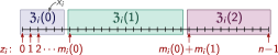
Figure 5: Partitioning of the range $\{0,\ldots,{n\!-\!1}\}$ into disjoint subranges ${\mathfrak{Z}}_{i}(x_{i})$, $x_{i}\in{\mathfrak{X}}_{i}$, see Eq. 9. The size of each subrange, $|{\mathfrak{Z}}_{i}(x_{i})|=m_{i}(x_{i})$, is proportional to the probability $Q_{i}(X_{i}\!=\!x_{i})$ (Eq. 8).

Figure 6: Encoding a symbol $x_{i}$ with ANS using the bits-back trick. The net bitrate is $\log_{2}n-\log_{2}m_{i}(x_{i})=-\log_{2}Q_{i}(X_{i}\!=\!x_{i})$.

Latent Variable Model.

Since the integers $m_{i}(x_{i})$ in Eq. 8 sum to $n$ for $x_{i}\in{\mathfrak{X}}_{i}$, they define a partitioning of the integer range $\{0,\ldots,n-1\}$ into $|{\mathfrak{X}}_{i}|$ disjoint subranges, see Figure 6: for each symbol $x_{i}\in{\mathfrak{X}}_{i}$, we define a subrange ${\mathfrak{Z}}_{i}(x_{i})\subseteq\{0,\ldots,n-1\}$ of size $|{\mathfrak{Z}}_{i}(x_{i})|=m_{i}(x_{i})$ as follows,

$$\textstyle{\mathfrak{Z}}_{i}(x_{i}):=\left\{\sum_{x_{i}^{\prime}<x_{i}}m_{i}(x_{i}^{\prime}),\;\;\ldots,\;\;\left(\sum_{x_{i}^{\prime}\leq x_{i}}m_{i}(x_{i}^{\prime})\right)-1\right\},$$ (9)

where we assumed some ordering on the alphabet ${\mathfrak{X}}_{i}$ (to define what “$x_{i}^{\prime}\!<\!x_{i}$” means). By construction, the subranges ${\mathfrak{Z}}_{i}(x_{i})$ are pairwise disjoint for different $x_{i}$ and they cover the entire range $\{0,\ldots,n-1\}$ (see Figure 6). Imagine now we want to draw a random sample $x_{i}$ from $Q_{i}$. A simple way to do this is to draw an auxiliary integer $z_{i}$ from a uniform distribution over $\{0,\ldots,n-1\}$, and then identify the unique symbol $x_{i}\in{\mathfrak{X}}_{i}$ that satisfies $z_{i}\in{\mathfrak{Z}}_{i}(x_{i})$. This procedure describes the so-called generative process of a latent variable model $Q_{i}(X_{i},Z_{i})=Q(Z_{i})\,Q_{i}(X_{i}\,|\,Z_{i})$ where

$$Q(Z_{i}\!=\!z_{i}) =\frac{1}{n}\;\;\forall z_{i}\in\{0,\ldots,n-1\}\,\quad\text{and}\,\quad Q_{i}(X_{i}\!=\!x_{i}\,|\,Z_{i}\!=\!z_{i})=\begin{cases}1&\!\!\text{if $z_{i}\in{\mathfrak{Z}}_{i}(x_{i})$;}\\ 0&\!\!\text{else.}\end{cases}$$ (10)

Using $|{\mathfrak{Z}}_{i}(x_{i})|=m_{i}(x_{i})$, one can easily verify that the approximated entropy model from Eq. 8 is the marginal distribution of the latent variable model from Eq. 10, i.e., our use of the same name $Q_{i}$ for both models is justified since we indeed have $Q_{i}(X_{i}\!=\!x_{i})=\sum_{z_{i}=0}^{n-1}Q_{i}(X_{i}\!=\!x_{i},Z_{i}\!=\!z_{i})\;\forall x_{i}\in{\mathfrak{X}}_{i}$.

The uniform prior distribution $Q(Z_{i})$ in Eq. 10 suggests that we could build a stream code by utilizing our UniformCoder from Listing 2. We begin with a naive approach upon which we then improve: to encode a message ${{\mathbf{x}}}=(x_{1},\ldots,x_{k})$, we simply identify each symbol $x_{i}$ by some $z_{i}$ that we may choose arbitrarily from ${\mathfrak{Z}}_{i}(x_{i})$, and we encode the resulting sequence $(z_{1},\ldots,z_{k})$ using a UniformCoder with alphabet $\{0,\ldots,n-1\}$. On the decoder side, we decode $(z_{1},\ldots,z_{k})$ and we recover the message ${{\mathbf{x}}}$ by identifying, for each $i$, the unique symbol $x_{i}$ that satisfies $z_{i}\in{\mathfrak{Z}}_{i}(x_{i})$.

The Bits-Back Trick.

Unfortunately, the above naive approach suffers from poor compression performance. Encoding $z_{i}$ with the uniform prior model $Q(Z_{i})$ increases the (amortized) bitrate by $z_{i}$’s information content, $-\log_{2}Q(Z_{i}\!=\!z_{i})=-\log_{2}\frac{1}{n}=\texttt{precision}$. By contrast, an optimal code would spend only $-\log_{2}Q_{i}(X_{i}\!=\!x_{i})=\texttt{precision}-\log_{2}m_{i}(x_{i})$ bits on symbol $x_{i}$ (see Eq. 8). Thus, our naive approach has an overhead of $\log_{2}m_{i}(x_{i})$ bits for each symbol $x_{i}$. The overhead arises because the encoder can choose $z_{i}$ arbitrarily among any element of ${\mathfrak{Z}}_{i}(x_{i})$, and this choice injects some information into the compressed bit string that is discarded on the decoder side. This suggests a simple solution, called the bits-back trick [Wallace, 1990, Hinton and Van Camp, 1993]: we should somehow utilize the $\log_{2}m_{i}(x_{i})$ bits of information contained in our choice of $z_{i}\in{\mathfrak{Z}}_{i}(x_{i})$, e.g., by communicating through it some part of the previously encoded symbols.

⬇

class SlowAnsCoder: # Has near-optimal bitrates but high runtime cost.

def __init__(self, precision, compressed=0):

self.n = 2**precision # See |Eq. \ref*{eq:approximatep}| (“|{\normalfont\texttt{**}}|” denotes exponentiation).

self.stack = UniformCoder(compressed) # Defined in Listing |\ref*{listing:pns}|.|\label{line:slow_ans_def_stack}|

\pardef push(self, symbol, m): # Encodes one symbol.

z = self.stack.pop(base=m[symbol]) + sum(m[0:symbol])|\label{line:slow_ans_push1}|

self.stack.push(z, base=self.n)|\label{line:slow_ans_push2}|

\pardef pop(self, m): # Decodes one symbol.

z = self.stack.pop(base=self.n)|\label{line:slow_ans_pop1}|

# Find the unique |$\mathtt{symbol}$| that satisfies |$\mathtt{z} \in\ZZ_i(\mathtt{symbol})$| (real deploy-

# ments should use a more efficient method than linear search):

for symbol, m_symbol in enumerate(m):|\label{line:slow_ans_find_symbol_begin}|

if z >= m_symbol:

z -= m_symbol

else:

break|\label{line:slow_ans_find_symbol_end}|

self.stack.push(z, base=m_symbol)|\label{line:slow_ans_pop2}|

return symbol

\pardef get_compressed(self):

return self.stack.number

Figure 7: A coder with near-optimal compression performance for arbitrary entropy models due to the bits-back trick (Section 3.2), but with poor runtime performance. Usage example in Listing 8.

Listing 7 implements this bits-back trick in a class SlowAnsCoder (a precursor to an AnsCoder that we will introduce in the next section). Like our UniformCoder, a SlowAnsCoder operates as a stack. The method push for encoding accepts a symbol $x_{i}$ from the (implied) alphabet ${\mathfrak{X}}_{i}={\{0,\ldots,\texttt{len(m)}-1\}}$, where the additional method argument “m” is a list of all the integers $m_{i}(x_{i}^{\prime})$ for $x_{i}^{\prime}\in{\mathfrak{X}}_{i}$, i.e., m specifies a model $Q_{i}$ (Eq. 8), and m[symbol] is $m_{i}(x_{i})$. The method body is very brief: Line LABEL:line:slow_ans_push1 in Listing 7 picks a $z_{i}\in{\mathfrak{Z}}_{i}(x_{i})$ and Line LABEL:line:slow_ans_push2 encodes $z_{i}$ onto a stack (which is a UniformCoder, see Line LABEL:line:slow_ans_def_stack) using a uniform entropy model over $\{0,\ldots,n-1\}$. The interesting part is how we pick $z_{i}$ in Line LABEL:line:slow_ans_push1: we decode $z_{i}$ from stack using the alphabet ${\mathfrak{Z}}_{i}(x_{i})$. Note that, at this point, we haven’t actually encoded $z_{i}$ yet; we just decode it from whatever data has accumulated on stack from previously encoded symbols (if any). This gives us no control over the value of $z_{i}$ except that it is guaranteed to lie within ${\mathfrak{Z}}_{i}(x_{i})$, which is all we need. Crucially, decoding $z_{i}$ consumes data from stack (see Figure 6), thus reducing the (amortized) bitrate as we analyze below.

The method pop for decoding inverts each step of push, and it does so in reverse order because we are using a stack. Line LABEL:line:slow_ans_pop1 in Listing 7 decodes $z_{i}$ using the alphabet $\{0,\ldots,n-1\}$ (thus inverting Line LABEL:line:slow_ans_push2) and Line LABEL:line:slow_ans_pop2 encodes $z_{i}$ using the alphabet ${\mathfrak{Z}}_{i}(x_{i})$ (thus inverting Line LABEL:line:slow_ans_push1). The latter step recovers the information that we communicate trough our choice of $z_{i}\in{\mathfrak{Z}}_{i}(x_{i})$ in push. The method pop may appear more complicated than push because it has to find the unique symbol $x_{i}$ that satisfies $z_{i}\in{\mathfrak{Z}}_{i}(x_{i})$, which is implemented here—for demonstration purpose—with a simple linear search (Lines LABEL:line:slow_ans_find_symbol_begin-LABEL:line:slow_ans_find_symbol_end). This search simultaneously subtracts $\sum_{x_{i}^{\prime}<x_{i}}m_{i}(x_{i}^{\prime})$ from $z_{i}$ before encoding it, which inverts the part of Line LABEL:line:slow_ans_push1 that adds sum(m[0:symbol]) to the value decoded from stack.

⬇

# Specify an approximated entropy model via |$\mathtt{precision}$| and |$m_i(x_i)$| from Eq. |\ref*{eq:approximatep}|:

precision = 4 # For demonstration; deployments should use higher |$\mathtt{precision}$|.|\label{line:set_precision}|

m = [7, 3, 6] # Sets |$Q_i(X_i\eq0) = \frac{7}{2^4}$|, |$Q_i(X_i\eq1) = \frac{3}{2^4}$|, and |$Q_i(X_i\eq2) = \frac{6}{2^4}$|.|\label{line:set_m}|

\par# Encode a message in |$\mathtt{reversed}$| order so we can decode it in forward order:

example_message = [2, 0, 2, 1, 0]|\label{line:ans_example_encode_begin}|

encoder = SlowAnsCoder(precision) # Also works with |$\mathtt{AnsCoder}$| (Listing |\ref*{listing:ans}|).

for symbol in reversed(example_message):|\label{line:ans_example_encoder_loop}|

encoder.push(symbol, m) # We could use a different |$\mathtt{m}$| for each |$\mathtt{symbol}$|.

compressed = encoder.get_compressed()

\par# We could actually reuse the |$\mathtt{encoder}$| for decoding, but let’s pretend that

# decoding occurs on a different machine that receives only “|$\mathtt{compressed}$|”.

decoder = SlowAnsCoder(precision, compressed)|\label{line:ans_example_decode_begin}|

reconstructed = [decoder.pop(m) for _ in range(5)]|\label{line:ans_example_decoder_loop}|

assert reconstructed == example_message # Verify correctness.|\label{line:ans_example_decode_end}|

Figure 8: Simple usage example for our SlowAnsCoder from Listing 7; the same example also works with our more efficient AnsCoder from Listing 3.3. For simplicity, we use the same entropy model $Q_{i}$ (Lines LABEL:line:set_precision-LABEL:line:set_m) for all symbols, but we could easily use an individual model for each symbol.

Listing 8 shows a usage example for SlowAnsCoder. For simplicity, we encode each symbol with the same model $Q_{i}$ here, but it would be straight-forward to use an individual model for each symbol.

⬇

class SlowAnsCoder: # Equivalent to Listing |\ref*{listing:slowans}|, just more self-contained.

def __init__(self, precision, compressed=0):

self.n = 2**precision # See |Eq. \ref*{eq:approximatep}| (“**” denotes exponentiation).

self.compressed = compressed # (== |$\mathtt{stack}$.$\mathtt{number}$| in |$\mathtt{SlowAnsCoder}$|)

\pardef push(self, symbol, m): # Encodes one symbol.

z = self.compressed self.compressed //= m[symbol] # “//” denotes integer division.|\label{line:slow_ans_inlined_push1b}|

self.compressed = self.compressed * self.n + z|\label{line:slow_ans_inlined_push2}|

\pardef pop(self, m): # Decodes one symbol.

z = self.compressed self.compressed //= self.n # “//” denotes integer division.|\label{line:slow_ans_inlined_pop1b}|

# Identify |{\normalfont\texttt{symbol}}| and subtract |{\normalfont\texttt{sum(m[0:symbol])}}| from |{\normalfont\texttt{z}}|:

for symbol, m_symbol in enumerate(m):|\label{line:slow_ans_inlined_find_symbol_begin}|

if z >= m_symbol:

z -= m_symbol

else:

break # We found the |$\mathtt{symbol}$| that satisfies |$\mathtt{z} \in\ZZ_i(\mathtt{symbol})$|.|\label{line:slow_ans_inlined_find_symbol_end}|

self.compressed = self.compressed * m_symbol + z|\label{line:slow_ans_inlined_pop2}|

return symbol

\pardef get_compressed(self):

return self.compressed

Figure 9: Reimplementation of SlowAnsCoder from Listing 7 where we removed the dependency on UniformCoder (Listing 2) by manually inlining the method calls stack.push() and stack.pop().

Correctness and Compression Performance.

Many researchers are initially confused by the bits-back trick. It may help to separately analyze its correctness and its compression performance. Correctness means that the method pop is the exact inverse of push, i.e., calling push(symbol, m) followed by pop(m) returns symbol and restores the SlowAnsCoder into its original state (assuming that all method arguments are valid, i.e., $0\leq\mathtt{symbol}<\texttt{len(m)}$ and $\texttt{sum(m)}=n=2^{\texttt{precision}}$). This can easily be verified by following the implementation in Listing 7 step by step. Crucially, it holds for any original state of the SlowAnsCoder, even if the coder starts out empty (i.e., with ${\texttt{compressed}=0}$). Some readers may find it easier to verify this by reference to Listing 9, which reimplements the SlowAnsCoder from Listing 7 in a self-contained way, i.e., without explicitly using a UniformCoder from Listing 2 because all method calls to stack are manually inlined.

The compression performance of a SlowAnsCoder is analyzed more easily in Listing 7. Line LABEL:line:slow_ans_push1 of the method push decodes $z_{i}$ from stack with a uniform entropy model over ${\mathfrak{Z}}_{i}(x_{i})$, i.e., with the model ${Q_{i}(Z_{i}\!=\!z_{i}\,|\,X_{i}\!=\!x_{i})}=1/m_{i}(x_{i})\;\forall z_{i}\in{\mathfrak{Z}}_{i}(x_{i})$. This reduces the (amortized) bitrate by the information content $-\log_{2}Q_{i}(Z_{i}\!=\!z_{i}\,|\,X_{i}\!=\!x_{i})=\log_{2}m_{i}(x_{i})$ bits, provided that at least this much data is available on stack (which holds for all but the first encoded symbol in a message). Line LABEL:line:slow_ans_push2 then encodes onto stack with a uniform entropy model over $\{0,\ldots,n-1\}$, which increases the bitrate by $\log_{2}n$. Thus, in total, encoding (pushing) a symbol $x_{i}$ contributes $\log_{2}\frac{n}{m_{i}(x_{i})}$ bits (see Figure 6), which is precisely the symbol’s information content, $-\log_{2}Q_{i}(X_{i}\!=\!x_{i})$ (see Eq. 8). Therefore, the SlowAnsCoder implements an optimal code for $Q$, except for the first symbol of the message, which always contributes $\log_{2}n=\mathtt{precision}$ bits (this constant overhead is negligible for long messages). However, the SlowAnsCoder turns out to be slow (as its name suggests), which we address next.

3.3 Computational Efficiency: The Practical (Streaming) ANS Algorithm

We speed up the SlowAnsCoder introduced in the last section (Listings 7 or 9), which finally leads us to the variant of ANS that is commonly used in practice (also called “streaming ANS”). While the SlowAnsCoder provides near-optimal compression performance, it is not a very practical algorithm because the runtime cost for encoding a message of length $k$ scales quadratically rather than linearly in $k$. This is because SlowAnsCoder represents the entire compressed bit string as a single integer (compressed in Listing 9), which would therefore become extremely large (typically millions of bits long) in practical applications such as image compression. The runtime cost of arithmetic operations involving compressed (Lines LABEL:line:slow_ans_inlined_push1a, LABEL:line:slow_ans_inlined_push1b, and LABEL:line:slow_ans_inlined_pop2 in Listing 9) thus scales linearly with the amount of data that has been compressed so far, leading to an overall cost of $O(k^{2})$ for a sequence of $k$ symbols.

To speed up the algorithm, we first observe that not all arithmetic operations on large integers are necessarily slow. Lines LABEL:line:slow_ans_inlined_push2, LABEL:line:slow_ans_inlined_pop1a, and LABEL:line:slow_ans_inlined_pop1b in Listing 9 perform multiplication, modulo, and integer division between compressed and $n$. Since $n=2^{\texttt{precision}}$ is a power of two (Eq. 8), this suggests storing the bits that represent the giant integer compressed in a dynamically sized array (aka “vector”) of precision-bit chunks (called “words” below) so that these arithmetic operations simplify to appending a zero word to the vector, inspecting the last word in the vector, and deleting the last word, respectively (analogous to how “$\times 10$”, “$\text{mod}~{}10$” and “$\lfloor\cdot/10\rfloor$” are trivial operations in the decimal system). A good vector implementation performs these operations in constant (amortized) runtime.

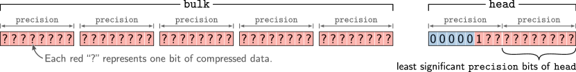
Figure 10: Streaming ANS with a growable bulk and a finite-capacity head. Encoding and decoding operate on head, but if encoding a symbol would overflow head then we first transfer the least significant precision bits of head to bulk. More general configurations are possible, see Section 4.1.

Unfortunately, the remaining arithmetic operations (Lines LABEL:line:slow_ans_inlined_push1a, LABEL:line:slow_ans_inlined_push1b, and LABEL:line:slow_ans_inlined_pop2 in Listing 9) cannot be reduced to a constant runtime cost because restricting $m_{i}(x_{i})$ to a power of two for all $x_{i}\in{\mathfrak{X}}_{i}$ would severely limit the expressivity of the approximated entropy model $Q$ (Eq. 8). The form of ANS that is used in practice (sometimes called “streaming ANS”) therefore employs a hybrid approach that splits the compressed bit string into a bulk and a head part (see Figure 10). The bulk holds most of the compressed data as a growable vector of fixed-sized words while the head has a relatively small fixed capacity (e.g., 64 bits). Most of the time, encoding and decoding operate only on head and thus have a constant runtime due to the bounded size of head. Only when head overflows or underflows certain thresholds (see below) do we transfer some data between head and the end of bulk. These transfers also have a constant (amortized) runtime because we always transfer entire words (see below).

Invariants.

We present here the simplest variant of streaming ANS, deferring generalizations to Section 4.1. In this variant, bulk is a vector of precision-bit words (i.e., unsigned integers smaller than $2^{\texttt{precision}}$), and head can hold up to ${2\!\times\!\texttt{precision}}$ bits (see Figure 10). The algorithm is very similar to our SlowAnsCoder from Listing 9 except that all arithmetic operations now act on head instead of compressed, and the encoder sometimes flushes some data from head to bulk while the decoder sometimes refills data from bulk to head. Obviously, the encoder and decoder have to agree on exactly when such data transfers occur. This is done by upholding the following invariants:

1. $\texttt{head}<2^{2\times\texttt{precision}}$, i.e., head is a ${2\!\times\!\texttt{precision}}$-bit unsigned integer; and

2. $\texttt{head}\geq 2^{\texttt{precision}}$ if bulk is not empty.

Any violation of these invariants triggers a data transfer between head and bulk that restores them.

class AnsCoder: def __init__(self, precision, compressed=[]): self.precision = precision self.mask = (1 << precision) - 1 # (a string of @$\mathtt{precision}$@ one-bits) self.bulk = compressed.copy() # (We will mutate @$\mathtt{bulk}$@ below.)@@ self.head = 0 # Establish invariant (ii): while len(self.bulk) != 0 and (self.head >> precision) == 0:@@ self.head = (self.head << precision) | self.bulk.pop()@@

def push(self, symbol, m): # Encodes one symbol. # Check if encoding directly onto @$\mathtt{head}$@ would violate invariant (i): if (self.head >> self.precision) >= m[symbol]:@@ # Transfer one word of compressed data from @$\mathtt{head}$@ to @$\mathtt{bulk}$@: self.bulk.append(self.head & self.mask) # (“@&@” is bitwise @and@)@@ self.head >>= self.precision@@ # At this point, invariant (ii) is definitely violated, # but the operations below will restore it.

z = self.head self.head //= m[symbol] self.head = (self.head << self.precision) | z # (This is@@ # equivalent to “@self.head * n + z@”, just slightly faster.)

def pop(self, m): # Decodes one symbol. z = self.head self.mask # (same as “@self.head self.head >>= self.precision # (same as “@//= n@” but faster) for symbol, m_symbol in enumerate(m):@@ if z >= m_symbol: z -= m_symbol else: break # We found the @$\mathtt{symbol}$@ that satisfies @$\mathtt{z}\in{\mathfrak{Z}}_{i}(\mathtt{symbol})$@.@@ self.head = self.head * m_symbol + z@@

# Restore invariant (ii) if it is violated (which happens exactly # if the encoder transferred data from @$\mathtt{head}$@ to @$\mathtt{bulk}$@ at this point): if (self.head >> self.precision) == 0 and len(self.bulk) != 0:@@ # Transfer data back from @$\mathtt{bulk}$@ to @$\mathtt{head}$@ (“@|@” is bitwise @or@): self.head = (self.head << self.precision) | self.bulk.pop()@@

return symbol

def get_compressed(self): compressed = self.bulk.copy() # (We will mutate @$\mathtt{compressed}$@ below.) head = self.head # Chop @$\mathtt{head}$@ into @$\mathtt{precision}$@-sized words and append to @$\mathtt{compressed}$@: while head != 0: compressed.append(head self.mask) head >>= self.precision return compressed

Figure 11: A complete streaming ANS entropy coder in Python. For a usage example, see Listing 8 (replace SlowAnsCoder with AnsCoder). This implementation is written in Python for demonstration purpose only. Real deployments should be implemented in a more efficient, compiled language (see, e.g., the constriction library presented in Section 5.1, which also provides Python bindings).

The Streaming ANS Algorithm.

Listing 3.3 shows the full implementation of our final AnsCoder, which is an evolution on our SlowAnsCoder implementation from Listing 9 (and which can be used as a replacement for SlowAnsCoder in the usage example of Listing 8). Method push checks upfront (on Line 3.3) if encoding directly onto head would lead to an overflow that would violate invariant (i). We show in Appendix A.1 that this is the case exactly if $\texttt{head}\,\texttt{>>}\,\texttt{precision}\geq m_{i}(x_{i})$, where “>>” denotes a right bit-shift (i.e., integer division by $2^{\texttt{precision}})$. If this is the case, then the encoder transfers the least significant precision bits from head to bulk (Lines 3.3-3.3). Since we assume that both invariants are satisfied at method entry, head initially contains at most ${2\!\times\!\texttt{precision}}$ bits (invariant (i)), so transferring precision bits out of it leads to a temporary violation of invariant (ii) (but both invariants hold again on method exit as we show in Appendix A.2). The temporary violation of invariant (ii) is on purpose: since transfers from head to bulk are the only operations during encoding that lead to a temporary violation of invariant (ii), we can detect and invert such transfers on the decoder side by simply checking for invariant (ii), see Lines 3.3-3.3 in Listing 3.3.

The method get_compressed exports the entire compressed data by concatenating bulk and head into a list of precision-bit words, which can be written to a file or network socket (e.g., by splitting each word into four 8-bit bytes if $\texttt{precision}=32$). Before we analyze the AnsCoder in more detail, we emphasize its simplicity: Listing 3.3 is a complete implementation of a computationally efficient entropy coder with very near-optimal compression performance (see below). By contrast, a complete implementation of arithmetic coding or range coding [Rissanen and Langdon, 1979, Pasco, 1976] would be much more involved due to a number of corner cases in those algorithms.

Compression Performance.

The separation between bulk and head reduces the runtime cost of ANS from quadratic to linear in the message length $k$, but it introduces a small compression overhead. When the encoder transfers data from bulk to head it simply chops off precision bits from the binary representation of head. This is well-motivated as we encode onto head with an optimal code (with respect to $Q$), and so one might assume that each valid bit in head carries one full bit of entropy. However, this is not quite correct: as discussed in Section 2.1, even with an optimal code, the expected length of the compressed bit string can exceed the entropy by up to almost $1$ bit. Thus, each valid bit in the binary representation of head carries slightly less than one bit of entropy.

According to Benford’s Law [Hill, 1995], the most significant (left) bits in head carry lowest entropy while less significant (right) bits are nearly uniformly distributed and thus indeed carry close to one bit of entropy each. This is why the transfer from head to bulk (Lines 3.3-3.3 in Listing 3.3) takes the least significant precision bits of head (see Figure 10). We can make their entropies arbitrarily close to one (and thus the overhead arbitrarily small) by increasing precision since a transfer occurs only if these bits are “buried below” at least an additional $\texttt{precision}-{(-\log_{2}Q_{i}(X_{i}\!=\!x_{i}))}$ valid bits.

In practice, streaming ANS has very close to optimal compression performance (see empirical results in Section 5.2 below). But a small bitrate-overhead over a hypothetical optimal coder comes from:

1. the linear (in $k$) overhead due to Benford’s Law just discussed (shrinks as precision increases);

2. a linear approximation overhead of $\sum_{i=1}^{k}D_{\text{KL}}(P_{i}\,||\,Q_{i})$ (shrinks as precision increases); and

3. a constant overhead of at most precision bits due the first symbol in the bits-back trick.

In practice, it is easy to find a precision that makes all three overheads negligibly small (see Section 5.2). But there can be additional constraints, e.g., memory alignment, the size of lookup tables for $Q_{i}$ (see Section 5.2), and the size of jump tables for random-access decoding (see Section 4.2).

Technical Details.

Listing 3.3 is an educational demo implementation of streaming ANS in the Python programming language. For efficiency, real deployments should use a language that provides more control over memory layout. We present an efficient open-source library (with pre-compiled bindings for Python) in Section 5.1 below. Further, Listing 3.3 replaces arithmetic operations that involve $n$ $(=2^{\texttt{precision}})$ by equivalent but faster bitwise operations. This allows us to avoid integer division when decoding, which is by far the slowest arithmetic operation on CPUs [Fog, 2021].

So far, we have ignored unique decodability (see Section 2.1). For a stream code like ANS, unique decodability is less important than for symbol codes since one rarely just concatenates the compressed representations of entire messages (e.g., entire compressed images) without using some container format or protocol. But we can easily make our AnsCoder from Listing 3.3 uniquely decodable by calling its constructor with argument compressed = [0, 1]. If we then encode a message, call get_compressed, concatenate the result to an arbitrary existing list of words $L^{\prime}$, and finally decode the message from this concatenation, then the decoder will end up with $\texttt{bulk}=L^{\prime}$ (and $\texttt{head}=n$).

This concludes our presentation of the basic algorithm for entropy coding with Asymmetric Numeral Systems (ANS). The next section discusses variations on this basic algorithm. Section 5 presents and empirically evaluates an optimized open-source library of various entropy coders (including ANS).

4 Variations on ANS

We generalize the basic streaming ANS algorithm from Section 3.3. The generalizations in Subsections 4.1 and 4.2 are straight-forward. Subsection 4.3 is more advanced, and it builds on our reinterpretation of ANS as bits-back coding with positional numeral systems presented in Section 3.2.

4.1 More General Streaming Configurations

Section 3.3 and Listing 3.3 present the simplest variant of streaming ANS. More general variants are possible. The bitlength of all words on bulk may be any integer $\texttt{word\_size}\geq\texttt{precision}$, and the head may have a more general bitlength $\texttt{head\_capacity}\geq\texttt{precision}+\texttt{word\_size}$. This includes the special case from Section 3.3 for $\texttt{word\_size}=\texttt{precision}$ and $\texttt{head\_capacity}=2\!\times\!\texttt{precision}$, but it also admits more general setups with the following generalized invariants:

1. $\texttt{head}<2^{\texttt{head\_capacity}}$, i.e., head can always be represented in head_capacity bits; and

2. $\texttt{head}\geq 2^{\texttt{head\_capacity}\,-\,\texttt{word\_size}}$ if bulk is not empty (a violation of this invariant means precisely that we can transfer one word from bulk to head without violating invariant (i’)).

Setting head_capacity larger than $\texttt{precision}+\texttt{word\_size}$ reduces overhead 1 from Section 3.3. We analyze this improvement empirically in Section 5.2. Setting word_size larger than precision may be motivated by more technical reasons, e.g., memory alignment of words on bulk and the memory footprint and thus cache friendliness of lookup tables for the quantile function of $Q_{i}$.

⬇

class SeekableAnsCoder: # Adds random-access decoding to Listing @\ref*{listing:ans}@.

# @{\normalfont\texttt{\_\_init\_\_}}@, @{\normalfont\texttt{push}}@, @{\normalfont\texttt{pop}}@, and @{\normalfont\texttt{get\_compressed}}@ same as in Listing @\ref*{listing:ans}@ …

\pardef checkpoint(self): # Records a point to which we can @$\mathtt{seek}$@ later.

return (len(self.bulk), self.head)

\pardef seek(self, checkpoint): # Jumps to a previously taken @$\mathtt{checkpoint}$@.

position, head = checkpoint

if position > len(self.bulk): # @$“\mathtt{raise}"$@ throws an exception.

raise "This simple demo can only seek forward."

self.bulk = self.bulk[0:position] # Truncates @$\mathtt{bulk}$@.

self.head = head

\par# Usage example:

precision = 4 # For demonstration; deployments should use higher @$\mathtt{precision}$@.

m = [7, 3, 6] # Same demo model as in Listing @\ref*{listing:ans_usage}@.

coder = SeekableAnsCoder(precision)

message = [2, 0, 2, 1, 0, 1, 2, 2, 2, 1, 0, 2, 1, 2, 0, 0, 1, 1, 1, 2]

\parfor symbol in reversed(message[10:20]): # Encode second half of @$\mathtt{message}$@.

coder.push(symbol, m)

checkpoint = coder.checkpoint() # Record a checkpoint.

for symbol in reversed(message[0:10]): # Encode first half of @$\mathtt{message}$@.

coder.push(symbol, m)

\parassert coder.pop(m) == message[0] # Decode first symbol.

assert coder.pop(m) == message[1] # Decode second symbol.

coder.seek(checkpoint) # Jump to 11th symbol.

assert [coder.pop(m) for _ in range(10)] == message[10:20] # Decode rest.

Figure 12: Streaming ANS with random-access decoding (see Section 4.2). This simple demo implementation can only seek forward since both seeking and decoding consume compressed data. To allow seeking backwards, one could use a cursor into immutable compressed data instead.

4.2 Random-Access Decoding

When decoding a compressed message, it is sometimes desirable to quickly jump to some specific position within the message (e.g., when skipping forward in a compressed video stream). Such random access is trivial in symbol codes as the decoder only needs to know the correct offset into the compressed bit string, which may be stored for selected potential jump targets as meta data (“jump table”) within some container format. For a stream code like ANS, jumping (or “seeking”) to a specific position within the message requires knowledge not only of the offset within the compressed bit string but also of the internal state that the decoder would have if it arrived at this position without seeking. ANS makes it particularly easy to obtain this target decoder state during encoding since—as opposed to, e.g., arithmetic coding—the encoder and decoder in ANS are the same data structure with the same internal state (i.e., head). Listing 12 shows an example of random access with ANS.

4.3 Continuity With Respect to Entropy Models

We now discuss a more specialized variation on ANS that may not be immediately relevant to most readers, but which demonstrates how useful a deep understanding of the ANS algorithm can be for developing new ideas. This is an advanced chapter. First time readers might prefer to skip to Section 5 for empirical results and practical advice in more common use cases before coming back here.

Streaming ANS as presented in Listing 3.3 is a highly effective algorithm for entropy coding with a fixed model. But the situation becomes tricker if modeling and entropy coding cannot be separated as clearly. For example, novel deep-learning based compression methods often employ probabilistic models over continuous spaces, and thus the models have to be discretized in some way before they can be used as entropy models. Advanced discretization methods might benefit from an end-to-end optimization on the encoder side that optimizes through the entropy coder. Unfortunately, optimizing a function that involves an entropy coder like ANS is extremely difficult since ANS packs as much information content into as few bits as possible, which leads to highly noncontinuous behavior.

⬇

precision = 4 # For demonstration; deployments should use higher @$\mathtt{precision}$@.

m_orig = [7, 3, 6] # Same demo entropy model as in Listing @\ref*{listing:ans_usage}@.

m_mod = [6, 4, 6] # (Slightly) modified entropy model compared to @{\normalfont\texttt{m\_orig}}@.

compressed = [0b1001, 0b1110, 0b0110, 0b1110] # Some example bit string.

\par# Case 1: decode 4 symbols using entropy model @{\normalfont\texttt{m\_orig}}@ for all symbols:

decoder = AnsCoder(precision, compressed) # @$\mathtt{AnsCoder}$@ defined in Listing @\ref*{listing:ans}@.

case1 = [decoder.pop(m_orig) for _ in range(4)]

\par# Case 2: change the entropy model, but *only* for the first symbol:

decoder = AnsCoder(precision, compressed) # “@$\mathtt{compressed}$@” hasn’t changed.

case2 = [decoder.pop(m_mod)] + [decoder.pop(m_orig) for _ in range(3)]

\parprint(f"case1 = {case1}") # Prints: “case1 = [0, 1, 0, 2]”

print(f"case2 = {case2}") # Prints: “case2 = [1, 1, 2, 0]”

# @$\;\!\uparrow$@ @$\;\nnwarrow$@ @$\nnwarrow$@

# We changed only the @$\mathtt{|}$@ But that affected both

# model for this symbol. @$\mathtt{|}$@ of these symbols too.

Figure 13: Non-local effects of entropy models (see Section 4.3); changing the entropy model for the first decoded symbol of a sequence leads to a ripple effect that may affect all subsequent symbols.

For example, Listing 13 demonstrates that ANS reacts in a very irregular and non-local way to even tiny changes of the entropy model. The example decodes a sequences of symbols from an example bit string compressed. Such a sequence of decoding operations could be part of a higher-level encoder that employs the bits-back trick on some latent variable model with a high-dimensional latent space. In this case, the encoder would still be allowed to optimize over certain model parameters (or, e.g., discretization settings) provided that it appends the final choice of those parameters to the compressed bit string before transmitting it. To demonstrate the effect of optimizing over model parameters, Listing 13 decodes from the same bit string twice. The employed entropy models differ slightly between these two iterations, but only for the first symbol. Yet, the decoded sequences differ not only on the first symbol but also on subsequent symbols that were decoded with identical entropy models.

This ripple effect is no surprise: changing the entropy model for the first symbol affects not only the immediately decoded symbol but also the internal coder state after decoding the first symbol, which in turn affects how the coder proceeds to decoding subsequent symbols. Our deeper understanding of ANS as a form of bits-back coding (see Section 3.2) allows us to pinpoint the problem more precisely as it splits the process of decoding a symbol $x_{i}$ into three steps: (1) decoding a number $z_{i}$ from the compressed data using the (fixed) alphabet $\{0,\ldots,{n-1}\}$; (2) identifying the unique symbol $x_{i}$ that satisfies $z_{i}\in{\mathfrak{Z}}_{i}(x_{i})$; and (3) encoding $z_{i}$ back onto the compressed data, this time using the (model-dependent) alphabet ${\mathfrak{Z}}_{i}(x_{i})$. Note that step (1) is independent of the entropy model. The only reason why changing the entropy model for one symbol affects subsequent symbols is step (3), which “leaks” information about the current entropy model to the stack of compressed data.

⬇

class ChainCoder: # Prevents the non-local effect shown in Listing @\ref*{listing:chain_coder_motivation}@.

def __init__(self, precision, compressed, remainders=[]):

"""Initializes a ChainCoder for decoding from ‘compressed‘."""

self.precision = precision

self.mask = (1 << precision) - 1

self.compressed = compressed.copy() # @$\mathtt{pop}$@ decodes from here.

self.remainders = remainders.copy() # @$\mathtt{pop}$@ encodes onto here.

self.remainders_head = 0

# Establish invariant (ii):

while len(self.remainders) != 0 and \ (self.remainders_head >> precision) == 0:

self.remainders_head <<= self.precision

self.remainders_head |= self.remainders.pop()

\pardef pop(self, m): # Decodes one symbol.

z = self.compressed.pop() # Always read a full word from @$\mathtt{compressed}$@.@\label{line:chain_pop_step1}@

for symbol, m_symbol in enumerate(m):@\label{line:chain_pop_step2_begin}@

if z >= m_symbol:

z -= m_symbol

else:

break # We found the @$\mathtt{symbol}$@ that satisfies @$\mathtt{z} \in\ZZ_i(\mathtt{symbol})$@.@\label{line:chain_pop_step2_end}@

\parself.remainders_head = self.remainders_head * m_symbol + z@\label{line:chain_pop_step3_begin}@

if (self.remainders_head >> (2 * self.precision)) != 0:

# Invariant (i) is violated. Flush one word to @{\normalfont\texttt{remainders}}@.

self.remainders.append(self.remainders_head & self.mask)

self.remainders_head >>= self.precision

# It can easily be shown that invariant (i) is restored here.@\label{line:chain_pop_step3_end}@

\parreturn symbol

\pardef push(self, symbol, m): # Encodes one symbol.

if len(self.remainders) != 0 and \ self.remainders_head < (m[symbol] << self.precision):

self.remainders_head <<= self.precision

self.remainders_head |= self.remainders.pop()

# Invariant (i) is now violated but will be restored below.

\parz = self.remainders_head self.remainders_head //= m[symbol]

self.compressed.append(z)

Figure 14: Sketch of an entropy coder that is similar to ANS but that prevents the non-local effect demonstrated in Listing 13 by using separate stacks of data for reading and writing (see Section 4.3).

This detailed understanding allows us to come up with an alternative entropy coder that does not exhibit the ripple effect shown in Listing 13. We can prevent the coder from leaking information about entropy models from one symbol to the next by using two separate stacks for the decoding and encoding operations in steps (1) and (3) above. Listing 14 sketches an implementation of such an entropy coder. The method pop decodes $z_{i}\in\{0,\ldots,{n-1}\}$ from compressed (Line LABEL:line:chain_pop_step1), identifies the symbol $x_{i}$ (Lines LABEL:line:chain_pop_step2_begin-LABEL:line:chain_pop_step2_end), and then encodes $z_{i}\in{\mathfrak{Z}}_{i}(x_{i})$ onto a different stack remainders (Lines LABEL:line:chain_pop_step3_begin-LABEL:line:chain_pop_step3_end). If we use this coder to decode a sequence of symbols (as in the example of Listing 13), then any changes to an entropy model for a single symbol affect only that symbol and the data that accumulates on remainders, but it has no effect on any subsequently decoded symbols. Once all symbols are decoded, one can concatenate compressed and remainders in an appropriate way.

As a technical remark, Listing 14 implements the simplest streaming configuration for such an entropy coder, with $\texttt{word\_size}=\texttt{precision}$ and $\texttt{head\_capacity}=2\!\times\!\texttt{precision}$. More general configurations analogous to Section 4.1 are possible and left as an exercise to the reader (hint: setting $\texttt{word\_size}>\texttt{precision}$ requires introducing a separate compressed_head).

In summary, our new perspective on ANS as bits-back coding with a UniformCoder allowed us to resolve a non-locality issue of ANS. While this specific issue is unlikely to be immediately relevant to most readers, other limitations of ANS might, and being able to semantically split ANS into the three subtasks of the bits-back trick might help overcome those too. This concludes our discussion of variations and generalizations of ANS. The next section provides some practical guidance on the streaming configuration based on empirically observed compression performances and runtime costs.

5 Software Library and Empirical Results

In this section, we briefly present an open-source library of various entropy coders (including ANS), we compare empirical bitrates and runtime costs for compressing real-world data across entropy coders and their configurations, and we provide practical advice based on these empirical results.

5.1 A Library of Entropy Coders for Research and Production

Data compression combines the procedural (i.e., algorithmic) task of entropy coding with the declarative task of probabilistic modeling. Recently, this separation of tasks has started to manifest itself also in the division of labor among researchers: systems and signal processing researchers are continuing to optimize compression algorithms for real hardware while machine learning researchers have started to introduce new ideas for the design of powerful probabilistic models (e.g., [Toderici et al., 2017, Minnen et al., 2018, Agustsson et al., 2020, Yang et al., 2020c, 2021]). Unfortunately, these two communities traditionally use vastly different software stacks, which seems to be slowing down idea transfer and thus might be part of the reason why machine-learning based compression methods are still hardly used in the wild despite their proven superior compression performance.

Along with this paper, the author is releasing constriction, an open-source library of entropy coders that intends to bridge the gap between systems and machine learning researchers by providing first-class support for both the Python and Rust programming language. To demonstrate constriction in a real deployment, we point readers to The Linguistic Flux Capacitor, a web application that uses constriction in a WebAssembly module to execute the neural compression method proposed in [Yang et al., 2020b] completely on the client side, i.e., in the user’s web browser.

Machine learning researchers can use constriction in their typical workflow through its Python API. It provides a consistent interface to various entropy coders, but it deliberately dictates the precise configuration of each coder in a way that prioritizes compression performance (at the cost of some runtime efficiency, see Section 5.2). This allows machine learning researchers to quickly pick a coder that fits their model architecture (e.g, a range coder for autoregressive models, or ANS for bits-back coding with latent variable models) without having to learn a new way of representing entropy models and bit strings for each coder type, and without having to research complex coder configurations.

Once a successful prototype of a new compression method is implemented and evaluated in Python, constriction’s Rust API simplifies the process of turning it into a self-contained product (i.e., an executable, static library or WebAssembly module). By default, constriction’s Rust and Python APIs are binary compatible, i.e., data encoded with one can be decoded with the other, which simplifies debugging. In addition, the Rust API optionally admits control (via compile-time type parameters) over coder details (streaming configurations, see Section 4.1, and data providers). This allows practitioners to tune a working prototype for optimal runtime and memory efficiency. The next section provides some guidance for these choices by comparing empirical bitrates and runtime costs.

5.2 Empirical Results and Practical Advice

We analyze the bitrates and runtime cost of Asymmetric Numeral Systems (ANS) with various streaming configurations (see Section 4.1), and we compare to Arithmetic Coding (AC) [Rissanen and Langdon, 1979, Pasco, 1976] and Range Coding (RC) [Martin, 1979]. We identify a streaming configuration where both ANS and RC are consistently effective over a large range of entropies, and we observe that that they are both considerably faster than AC. Based on these findings, we provide practical advice for when and how to use which entropy coding algorithm.

Benchmark Data.

We test all entropy coders on the data that are decoded in The Linguistic Flux Capacitor web app (see footnote 9 on page 9), which are the discretized model parameters of the natural language model from [Bamler and Mandt, 2017]. We chose these discretized model parameters as benchmark data because they arose in a real use case and they cover a wide spectrum of entropies per symbol spanning four orders of magnitude. The model parameters consist of 209 slices of 3 million parameters each. We treat the symbols within each slice as i.i.d. and use the empirical symbol frequencies within each slice as the entropy model when encoding and decoding the respective slice. Before discretization, the model parameters were transformed such that each slice represents the difference from other slices of varying distance (similar to I- and B-frames in a video codec). This leads to a wide range of entropies, ranging from about $0.001$ to $10$ bits per symbol from the lowest to highest entropy slice (with an overall average of $0.41$ bits per symbol).

Experiment Setup.

We use the proposed constriction library through its Rust API for both ANS and RC, and the third-party Rust library arcode [Burgess, ] for AC. In the following, we specify the streaming configuration (see Section 4.1) for ANS and RC by the triple “$\texttt{precision}\,/\,\texttt{word\_size}\,/\,\texttt{head\_capacity}$”. These parameters can be set in constriction’s Rust API at compile time so that the compiler can generate optimized code for each configuration. The library defines two presets: “default” (${24\,/\,32\,/\,64}$), which is recommended for initial prototyping (and therefore exposed through the Python API), and “small” (${12\,/\,16\,/\,32}$), which is optimized for runtime and memory efficiency. In addition to these two preset configurations, we also experiment with ${32\,/\,32\,/\,64}$ and ${16\,/\,16\,/\,32}$, which match the simpler setup of Section 3.3 (i.e., $\texttt{precision}=\texttt{word\_size}$). For AC, the only tuning parameter is the fixed-point precision. We report results with $\texttt{precision}=63$ (the highest precision supported by arcode) since lowering the precision did not improve runtime performance. Our benchmark code and data is available online.

The reported runtime for each slice is the median over 10 measurements on an Intel Core i7-7500U CPU (2.70 GHz) running Ubuntu Linux 21.10. We ran an entire batch of experiments (encoding and decoding all slices with all tested entropy coders) in the inner loop and repeated this procedure 10 times, randomly shuffling the order of experiments for each of the 10 batches. For each experiment, we encoded/decoded the entire slice twice in a row and measured only the runtime of the second run, so as to minimize variations in memory caches and branch predictions. We calculated and saved a trivial checksum (bitwise xor) of all decoded symbols to ensure that no parts of the decoding operations were optimized out. The benchmark code was compiled with constriction version 0.1.4, arcode version 0.2.3, and Rust version 1.57 in --release mode and ran in a single thread.

Table 1: Empirical compression performances and runtimes of Asymmetric Numeral Systems (ANS), Range Coding (RC), and Arithmetic Coding (AC); ANS and RC use the proposed constriction library, which admits arbitrary streaming configurations (see Section 4.1). Python bindings are provided for both ANS and RC for the configurations labeled as “default” in this table, which both have negligible ($<0.1\,\%$) bitrate overhead while being considerably faster than arithmetic coding.

Method $(\texttt{precision}\,/$	Bitrate overhead over Eq. 1			Runtime [ns per symbol]
$\texttt{word\_size}\,/\,\texttt{head\_capacity})$	$\blacktriangleright$ total	$\blacktriangleright\!D_{\text{KL}}(P\,||\,Q)$		$\blacktriangleright$ encoding	$\blacktriangleright$ decoding
ANS $(24\,/\,32\,/\,64)$ (“default”)	$0.0015\,\%$	$2.6\!\times\!10^{-6}\,\%$		$24.2$	$~{}~{}6.1$
ANS $(32\,/\,32\,/\,64)$	$0.0593\,\%$	$<10^{-8}\,\%$		$24.2$	$~{}~{}6.9$
ANS $(16\,/\,16\,/\,32)$	$0.2402\,\%$	$0.1235\,\%$		$19.8$	$~{}~{}6.4$
ANS $(12\,/\,16\,/\,32)$ (“small”)	$3.9567\,\%$	$3.9561\,\%$		$19.8$	$~{}~{}6.9$
RC $(24\,/\,32\,/\,64)$ (“default”)	$0.0237\,\%$	$2.6\!\times\!10^{-6}\,\%$		$16.6$	$14.3$
RC $(32\,/\,32\,/\,64)$	$1.6089\,\%$	$<10^{-8}\,\%$		$16.7$	$14.8$
RC $(16\,/\,16\,/\,32)$	$3.4950\,\%$	$0.1235\,\%$		$16.9$	$~{}~{}9.4$
RC $(12\,/\,16\,/\,32)$ (“small”)	$4.5807\,\%$	$3.9561\,\%$		$16.8$	$~{}~{}9.4$
Arithmetic Coding (AC)	$0.0004\,\%$	n/a		$43.2$	$85.6$

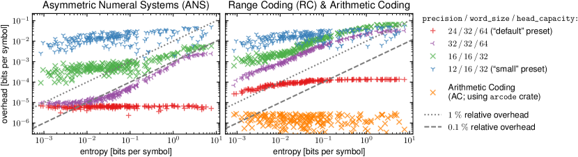
Figure 15: Empirical compression performances (bitrate overhead over Eq. 1) of various entropy coders as a function of entropy per symbol in each slice of the benchmark data. The “default” presets (red) for ANS and RC have a consistently low overhead over a wide range of entropies. The “small” presets (blue) may be advantageous in memory or runtime-constrained situations (see also Figure 16).

Results 1: Bitrates.

Table 1 shows aggregate empirical results over all slices of the benchmark data; A bitrate overhead of $1\,\%$ in the second column would mean that the number of bits produced by a coder when encoding the entire benchmark data is $1.01$ times the total information content of the benchmark data. We observe that arithmetic coding has the lowest bitrate overhead as expected, but the “default” preset for both ANS and RC in constriction has negligible ($<0.1\,\%$) overhead too on this data set. Interestingly, setting precision slightly smaller than word_size is beneficial for overall compression performance, suggesting a Benford’s Law contribution to the overhead (see Section 3.3). Reducing the precision increases the overhead, and the third column of Table 1 reveals that the overhead in the low-precision regime is largely due to the approximation error $D_{\text{KL}}(P\,||\,Q)$. Figure 15 breaks down the overhead for each of the 209 slices in the data set, plotting them as a function of the entropy in each slice. We observe that the “default” preset (red plus markers) provides the consistently best bitrates within each method over a wide range of entropies, which is why constriction’s Rust and Python APIs guide users to use this preset for initial prototyping.

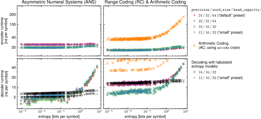
Figure 16: Measured runtimes for encoding (top) and decoding (bottom) as a function of the entropy per symbol. Models with low precision admit tabulating the mapping $z_{i}\mapsto x_{i}:z_{i}\in{\mathfrak{Z}}_{i}(x_{i})$ for all $z_{i}\in\{0,\ldots,{2^{\texttt{precision}}-1}\}$, which speeds up decoding in the high-entropy regime (gray markers).

Results 2: Runtimes.

The last two columns in Table 1 list the runtime cost (in nanoseconds per symbol) for encoding and decoding, averaged over the entire benchmark data. We observe that ANS provides the fastest decoder while RC provides the fastest encoder. In the “default” preset, decoding with ANS is more than twice as fast compared to RC. AC is much slower than both ANS and RC for both encoding and decoding in our experiments. While the precise runtimes reported here should be taken with a grain of salt since they depend on the specific implementation of each algorithm, one can generally expect AC to be considerably slower than ANS and RC since it reads and writes compressed data bit by bit, which is a poor fit for modern hardware. Indeed, Figure 16, which plots runtimes as a function of entropy in the respective slice of the benchmark data, reveals that AC (orange crosses) slows down in the high-entropy regime, i.e., when it has to read or write many bits per symbol.

While the encoder runtimes for ANS and RC (upper panels in Figure 15) depend only weakly on the entropy, decoding with ANS and RC slows down in the high-entropy regime. The main computational cost in this regime turns out to be the task of identifying the symbol $x_{i}$ that satisfies $z_{i}\in{\mathfrak{Z}}_{i}(x_{i})$ (corresponding to Lines 3.3-3.3 in Listing 3.3). For categorical entropy models like the ones used here, constriction uses a binary search here by default, which tends to require more iterations in models with high entropy. The library therefore provides an alternative way to represent categorical entropy models that tabulates the mapping $z_{i}\mapsto x_{i}$ for all $z_{i}\in\{0,\ldots,n-1\}$ upfront, leading to a constant lookup time. Since the size of such lookup tables is proportional to $n=2^{\texttt{precision}}$, they are only viable for low precisions (gray crosses and Y-shaped markers in the bottom panels in Figure 16). We observe that tabulated entropy models indeed speed up decoding in the high-entropy regime but they come at a cost in the low entropy regime (likely because large lookup tables are not cache friendly).

Practical Advice.

In summary, the Asymmetric Numeral Systems (ANS) algorithm reviewed in this paper, as well as Range Coding (RC), both provide very close to optimal bitrates while being considerably faster than Arithmetic Coding. While the precise bitrates and runtimes differ slightly between ANS and RC, in practice, it is usually more important to pick an entropy coder that fits the model architecture: RC operates as a queue (first-in-first-out), which simplifies compression with autoregressive models, while ANS operates as a stack (last-in-first-out), which simplifies bits-back coding with latent variable models. Both ANS and RC can be configured by parameters that trade off compression performance against runtime and memory efficiency. Users of the constriction library are advised to use the configuration from the “default” preset for initial prototyping (as guided by the API), and to tune the configuration only once they have implemented a working prototype.

6 Conclusion

We provided an educational discussion of the Asymmetric Numeral Systems (ANS) entropy coder, explaining the algorithm’s internals using concepts that are familiar to many statisticians and machine-learning scientists. This allowed us to understand Asymmetric Numeral Systems as a generalization of Positional Numeral Systems, and as an application of the bits-back trick. Splitting up ANS into the three distinct steps of the bits-back trick allowed us to generalize the method by combining these three steps in new ways. We hope that more idea transfer like this between the procedural (algorithmic) and the declarative (modeling) subcommunities within the field of compression research will spark novel ideas for compression methods in the future.

From a more practical perspective, we presented constriction, a new open-source software library that provides a collection of effective and efficient entropy coders and adapters for defining complex entropy models. The library is intended to simplify compression research (by providing a catalog of several different entropy coders within a single consistent framework) and to speed up the transition from research code to self-contained software products (by providing binary compatible entropy coders for both Python and Rust). We showed empirically that the entropy coders in constriction have very close to optimal compression performance while being much faster than Arithmetic Coding.

Acknowledgments

The author thanks Tim Zhenzhong Xiao for stimulating discussions and Stephan Mandt for important feedback. This work was supported by the German Federal Ministry of Education and Research (BMBF): Tübingen AI Center, FKZ: 01IS18039A. Robert Bamler is a member of the Machine Learning Cluster of Excellence, funded by the Deutsche Forschungsgemeinschaft (DFG, German Research Foundation) under Germany’s Excellence Strategy – EXC number 2064/1 – Project number 390727645. The author thanks the International Max Planck Research School for Intelligent Systems (IMPRS-IS) for support.

Appendix A Appendix: Proof of Correctness of Streaming ANS

We prove that the AnsCoder from Listing 3.3 of the main text implements a correct encoder/decoder pair, i.e., that its methods push and pop are inverse to each other. The proof uses that the AnsCoder upholds the two invariants (i) and (ii) from Section 3.3 of the main text, which we also prove.

Assumptions and Problem Statement.

We assume that the AnsCoder is used correctly: the constructor (“__init__”) must be called with a positive integer precision and its optional argument compressed, if given, must be a list of nonnegative integers that are all smaller than $n=2^{\texttt{precision}}$). Once the AnsCoder is constructed, its methods push and pop may be called in arbitrary order and repetition to bring the AnsCoder into some original state $S_{0}$. In this initial setup phase that establishes state $S_{0}$, the employed entropy models (argument m in both push and pop) may vary arbitrarily across method calls and do not have to match between any of the push and pop calls, but they do have to specify valid entropy models (i.e., each m must be a nonempty list of nonnegative integers that sum to $n$). Further, the argument symbol of each push call must be a nonnegative integer that is smaller than the length of the corresponding m, and it must satisfy $\texttt{m[symbol]}\neq 0$ (ANS cannot encode symbols with zero probability under the approximated entropy model $Q_{i}$). Once state $S_{0}$ is established, we consider two scenarios:

1. we call push(symbol, m) with an arbitrary $\texttt{symbol}\in\{0,\ldots,\texttt{len(m)}\}$, followed by pop(m) with the same (valid) model m; or

2. we call pop(m), assign the return value to a variable symbol, and then call push(symbol, m) with the returned symbol and the same (valid) model m.

We show that, after executing either of the above two scenarios, the AnsCoder ends up back in state $S_{0}$. For scenario (a), we further show that the final pop returns the symbol that was used in the preceding push. In Subsection A.1, we prove these claims under the assumption that the two invariants (i) and (ii) from Section 3.3 of the main text hold at entry of all methods. In Subsection A.2, we show that AnsCoder indeed upholds these two invariants (for completeness, the invariants are: (i) $\texttt{head}<n^{2}$ (always) and (ii) $\texttt{head}\geq n$ if bulk is not empty, where $n=2^{\texttt{precision}}$).

A.1 Proof of Correctness, Assuming Invariants are Upheld

To simplify the discussion, we conceptually split the method push into two parts, conditional_flush (Lines 3.3-3.3 in Listing 3.3 of the main text) followed by push_onto_head (Lines LABEL:line:ans_regular_push_begin-3.3). Similarly, we conceptually split the method pop into pop_from_head (Lines LABEL:line:ans_regular_pop_begin-3.3) followed by conditional_refill (Lines 3.3-3.3). The parts push_onto_head and pop_from_head are analogous to the push and pop method, respectively, of the SlowAnsCoder (Listing 9), and it is easy to see that they are inverse to each other (regardless of whether or not invariants (i) and (ii) hold). The tricker part is to show that the conditional flushing and refilling happen consistently, i.e., either none or both of them occur.

Scenario (a):

Scenario (a) executes the sequence conditional_flush, push_onto_head, pop_from_head, conditional_refill. Since the second and third step are inverse to each other, this simplifies to: starting from the original state $S_{0}$; then executing conditional_flush, which brings the AnsCoder into a new state $S^{\prime}$; and then executing conditional_refill. We show that the final state is again $S_{0}$ (this also shows that the symbol returned by the final pop is the one used in the call to push, since the problem effectively reduces to a SlowAnsCoder). Both conditional_flush and conditional_refill are predicated on some condition (see if-statements on Lines 3.3 and 3.3, respectively), and each part is a no-op if its respective condition is not met. Thus, if the condition for conditional_flush is not satisfied, then $S^{\prime}=S_{0}$, which satisfies invariant (ii) by assumption. The condition for conditional_refill checks precisely for violation of invariant (ii), so conditional_refill also becomes a no-op in this case, and we trivially end up in state $S_{0}$. If, on the other hand, the condition for conditional_flush is satisfied, then it is easy to see that $S^{\prime}$ violates invariant (ii): line 3.3 ensures that bulk is not empty and line 3.3 performs a right bit-shift of head by precision, which sets $\texttt{head}_{S^{\prime}}=\lfloor\texttt{head}_{S_{0}}/2^{\texttt{precision}}\rfloor$ (where subscripts denote the coder state in which we evaluate a variable). Since $S_{0}$ satisfies invariant (i) by assumption, we have $\texttt{head}_{S_{0}}<2^{2\times\texttt{precision}}$, and so $\texttt{head}_{S^{\prime}}<2^{\texttt{precision}}$, which (temporarily) violates invariant (ii). This means that the condition for conditional_refill is satisfied, and it is easy to see that Line 3.3 inverts Lines 3.3-3.3. Thus, Scenario (a) restores the AnsCoder into its original state $S_{0}$.

Scenario (b):

Calling pop before push leads to the folowing state transition:

$$S_{0}\xrightarrow{\;\texttt{pop\_from\_head}\;}S_{1}\xrightarrow{\;\texttt{conditional\_refill}\;}S_{2}\xrightarrow{\;\texttt{conditional\_flush}\;}S_{3}\xrightarrow{\;\texttt{push\_onto\_head}\;}S_{4}.$$ (A1)

We show that state $S_{4}=S_{0}$. Since push_onto_head is the inverse of pop_from_head, it suffices to show that $S_{3}=S_{1}$. Note that we can assume the invariants only about $S_{0}$. The intermediate state $S_{1}$ may violate invariant (ii), but it is easy to see that it satisfies invariant (i): Lines LABEL:line:ans_regular_pop_begin-3.3 set

$$\texttt{head}_{S_{1}}=\left\lfloor\frac{\texttt{head}_{S_{0}}}{n}\right\rfloor\times m_{i}(x_{i})+z_{i}^{\prime}$$ (A2)

with $z_{i}^{\prime}=z_{i}-\sum_{x_{i}^{\prime}<x_{i}}m_{i}(x_{i}^{\prime})$ where $z_{i}=(\texttt{head}_{S_{0}}\,\text{mod}\,n)$ is the value that gets initialized on Line LABEL:line:ans_regular_pop_begin. Since Lines 3.3-3.3 find the symbol $x_{i}$ that satisfies $z_{i}\in{\mathfrak{Z}}_{i}(x_{i})$, we have $z_{i}<\sum_{x_{i}^{\prime}\leq x_{i}}m_{i}(x_{i}^{\prime})$ (see Eq. 9 of the main text) and thus $z_{i}^{\prime}<m_{i}(x_{i})$. Further, we have $\texttt{head}_{S_{0}}<n^{2}$ by invariant (i). Thus, we find the upper bound

$$\texttt{head}_{S_{1}} \leq\left\lfloor\frac{n^{2}-1}{n}\right\rfloor\times m_{i}(x_{i})+(m_{i}(x_{i})-1)$$

$$=(n-1)m_{i}(x_{i})+m_{i}(x_{i})-1$$

$$=n\,m_{i}(x_{i})-1.$$ (A3)

Since the $m_{i}(x_{i}^{\prime})$ are nonnegative for all $x_{i}^{\prime}$ and sum to $n$, we have $m_{i}(x_{i})\leq n$, and so Eq. A3 implies $\texttt{head}_{S_{1}}<n^{2}$, and thus $S_{1}$ satisfies invariant (i). We now distinguish two cases depending on whether $S_{1}$ satisfies invariant (ii). If $S_{1}$ satisfies invariant (ii), then conditional_refill is a no-op and $S_{2}=S_{1}$. In the next step, conditional_flush checks whether $\lfloor\texttt{head}_{S_{1}}/n\rfloor\geq m_{i}(x_{i})$ on Line 3.3, which cannot be the case due to Eq. A3, and thus conditional_flush is also a no-op and we have $S_{3}=S_{2}=S_{1}$. If, on the other hand, $S_{1}$ does not satisfy invariant (ii), then bulk was not empty at the entry of the method pop, and thus the assumption that the original state $S_{0}$ satisfies invariant (ii) implies $\texttt{head}_{S_{0}}\geq n$. Line 3.3 then sets head to the new value $\texttt{head}_{S_{2}}=\texttt{head}_{S_{1}}\times n+b$ with some $b\geq 0$. In the next step, conditional_flush checks whether $\lfloor\texttt{head}_{S_{2}}/n\rfloor\geq m_{i}(x_{i})$, which is now indeed the case since $\lfloor\texttt{head}_{S_{2}}/n\rfloor\geq\lfloor\texttt{head}_{S_{1}}\times n/n\rfloor=\texttt{head}_{S_{1}}$, which is at least $m_{i}(x_{i})$ according to Eq. A2 since $\texttt{head}_{S_{0}}\geq n$ in this case. The flushing operation on Lines 3.3-3.3 is thus executed and it inverts the refilling operation from Line 3.3, and we again have $S_{3}=S_{1}$, as claimed. Thus, Scenario (b) also restores the AnsCoder into its original state $S_{0}$.

A.2 Proof That Invariants Are Uphold

The above prove of correctness relied on the assumption that invariants (i) and (ii) from Section 3.3 of the main text always hold at the entry of methods push and pop. We now show that this assumption is justified by proving that the constructor initializes an AnsCoder into a state that satisfies both invariants, and that all methods uphold the invariants (i.e., both invariants hold on method exit provided that they hold on method entry).

Constructor.

It is easy to see that both invariants are satisfied when the constructor finishes: the loop condition on Line 3.3 of Listing 3.3 checks if invariant (ii) is violated, i.e., if bulk is empty and $\texttt{head}<n$ (the latter is equivalent to $\texttt{head}\,{\texttt{>>}\,\texttt{precision}=0}$ where >> denotes a right bit-shift, i.e., integer division by $n=2^{\texttt{precision}}$). The loop thus only terminates once invariant (ii) is satisfied (it is guaranteed to terminate since the loop body on Line 3.3 pops a word from bulk and the loop terminates at latest once bulk is empty). Invariant (i) is satisfied throughout the constructor since head is initialized as zero (which is smaller than $n^{2}$) and the only statement that mutates head in the constructor is Line 3.3. This statement is only executed if head has at most precision valid bits, and it increases the number of valid bits by at most precision (due to the left bit-shift <<), so it can never lead to more than $2\times\texttt{precision}$ valid bits, which would be necessary to violate invariant (i).

Encoding.

We now analyze the method push in Listing 3.3 of the main text. Assuming that both invariants hold at method entry, we denote by $h$ and $h^{\prime}$ the value of head at method entry and exit, respectively, and we distinguish two cases depending on whether or not the if-condition on Line 3.3 is met.

• If the if-condition on Line 3.3 is met then we have

  $$h\,\texttt{>>}\,\texttt{precision}\geq m_{i}(x_{i})\quad\text{and}\quad h^{\prime}=\left(\left\lfloor\frac{h\,\texttt{>>}\,\texttt{precision}}{m_{i}(x_{i})}\right\rfloor\texttt{<<}\,\texttt{precision}\right)+z_{i}$$ (A4)

  with $z_{i}\in\{0,\ldots,2^{\texttt{precision}}-1\}$ (which is why the addition in Eq. A4 can be implemented as a slightly faster bitwise “or” in the code). Using $n=2^{\texttt{precision}}$, we can rewrite the right and left bit shifts in Eq. A4 as integer division by $n$ (rounding down) and multiplication with $n$, respectively. Thus, Eq. A4 simplifies to

  $$\left\lfloor\frac{h}{n}\right\rfloor\geq m_{i}(x_{i})\qquad\text{and}\qquad h^{\prime}=\left\lfloor\frac{\lfloor h/n\rfloor}{m_{i}(x_{i})}\right\rfloor\times n+z_{i}$$ (A5)

  Combining both parts of Eq. A5, we find

  $$h^{\prime}\geq\left\lfloor\frac{m_{i}(x_{i})}{m_{i}(x_{i})}\right\rfloor\times n+z_{i}\geq n=2^{\texttt{precision}}$$ (A6)

  and thus invariant (ii) is satisfied at method exit. To show that invariant (i) is also satisfied at method exit, we start from the assumption that invariant (i) holds at method entry, i.e., $h<n^{2}$. Therefore, we have $h/n<n$ and thus $\lfloor h/n\rfloor\leq n-1$ (since $n$ is an integer). Inserting this into the second part of Eq. A5 leads to

  $$h^{\prime}\leq\left\lfloor\frac{n-1}{m_{i}(x_{i})}\right\rfloor\times n+z_{i}\stackrel{{\scriptstyle(*)}}{{\leq}}(n-1)\times n+z_{i}=n^{2}-(n-z_{i})<n^{2}$$ (A7)

  where, in the equality marked with “$(*)$”, we used that $m_{i}(x_{i})>0$ for the encoded symbol $x_{i}$ by assumption (and thus $m_{i}(x_{i})\geq 1$ since $m_{i}(x_{i})$ is an integer). In the last equality, we used $z_{i}<n$. Thus, invariant (i) is also satisfied at method exit.

• If the if-condition on Line 3.3 is not met we have

  $$\left\lfloor\frac{h}{n}\right\rfloor<m_{i}(x_{i})\qquad\text{and}\qquad h^{\prime}=\left\lfloor\frac{h}{m_{i}(x_{i})}\right\rfloor\times n+z_{i}.$$ (A8)

  We can simplify the first part of Eq. A8 to $h/n<m_{i}(x_{i})$ since $m_{i}(x_{i})$ is an integer, and we thus find $h/m_{i}(x_{i})<n$ (using the fact that $m_{i}(x_{i})\neq 0$ by assumption for the encoded symbol $x_{i}$) and thus $\lfloor h/m_{i}(x_{i})\rfloor\leq n-1$. Inserting into the second part of Eq. A8 leads to

  $$h^{\prime}\leq(n-1)\times n+z_{i}=n^{2}-(n-z_{i})<n^{2}$$ (A9)

  where we agin used $z_{i}<n$ in the final step. Thus invariant (i) is satisfied at method exit. Regarding invariant (ii), we note that $m_{i}(x_{i})\leq n$ since $\sum_{x_{i}^{\prime}\in{\mathfrak{X}}_{i}}m_{i}(x_{i}^{\prime})=n$, where all terms in the sum are nonnegative. Thus, the smallest we can make $h^{\prime}$ in Eq. A8 is if we set $m_{i}(x_{i})=n$ and $z_{i}=0$, which results in the lower bound

  $$h^{\prime}\geq\left\lfloor\frac{h}{n}\right\rfloor\times n.$$ (A10)

  Assuming that invariant (ii) holds at method entry, we know that either bulk is empty, in which case it remains empty at method exit (since we’re considering the case where the if-condition on Line 3.3 is not met, in which case we don’t mutate bulk); or $h\geq n$ which, combined with Eq. A10 implies that $h^{\prime}>n$. Thus, either way, invariant (ii) remains satisfied at method exit.

Decoding.

We finally analyze the method pop in Listing 3.3 of the main text. We show that calling pop(m) upholds invariants (i) and (ii) (regardless of whether or not it follows a call of push(symbol, m) with the same m). We denote the value of head at entry of the method push by capital letter $H$ so that there is no confusion with the discussion of push. Once the program flow reaches Line 3.3, head takes the (intermediate) value

$$\tilde{H}=\left\lfloor\frac{H}{n}\right\rfloor\times m_{i}(x_{i})+z_{i}^{\prime}$$ (A11)

where $z_{i}^{\prime}\in\{0,\ldots,m_{i}(x_{i})-1\}$ and $x_{i}$ is the decoded symbol, which implies that ${\mathfrak{Z}}_{i}(x_{i})$ is not empty and therefore $m_{i}(x_{i})=|{\mathfrak{Z}}_{i}(x_{i})|\geq 1$. It is easy to see that $\tilde{H}<n^{2}$, i.e., $\tilde{H}$ satisfies invariant (i) since the largest we can make $\tilde{H}$ in Eq. A11 is by setting $H=n^{2}-1$ (the largest value allowed by invariant (i)), $m_{i}(x_{i})=n$, and $z_{i}^{\prime}=n-1$. This leads to the upper bound

$$\tilde{H}\leq\left\lfloor\frac{n^{2}-1}{n}\right\rfloor\times n+(n-1)=(n-1)\times n+(n-1)=n^{2}-1<n^{2}.$$ (A12)

The if-condition on Line 3.3 checks if invariant (ii) is violated. We again distinguish two cases:

• If invariant (ii) holds on Line 3.3 then the method exits, and thus both invariants hold on method exit.

• If invariant (ii) does not hold on Line 3.3 then the if-branch is taken and Line 3.3 mutates head into the final state

  $$H^{\prime}=\tilde{H}\times n+b$$ (A13)

  where $b\in\{0,\ldots,n-1\}$ is the word of data that was transferred from bulk. We can see directly that $H^{\prime}$ satisfies invariant (i) since, as $\tilde{H}$ violates invariant (ii) we have $\tilde{H}\leq n-1$ and therefore $H^{\prime}\leq(n-1)\times n+b=n^{2}+(b-n)<n^{2}$ since $b<n$. Regarding invariant (ii), we first note that invariant (ii) can only be violated on Line 3.3 if bulk at method entry is nonempty. Thus, the assumption that invariant (ii) is satisfied at method entry implies that $H\geq n$. This allows us to see that $\tilde{H}\neq 0$ since both $\lfloor H/n\rfloor$ and $m_{i}(x_{i})$ are nonzero in Eq. A11. Inserting into Eq. A13 leads to $H^{\prime}\geq n$, i.e., invariant (ii) is also satisfied at method exit.

In summary, we proved that the AnsCoder from Listing 3.3 of the main text upholds the two invariants stated in Section 3.3 of the main text. Using this property, we proved in Section A.1 that the AnsCoder is a correct encoder/decoder, i.e., that pop is both the left- and the right-inverse of push.

References

- Duda et al. [2015] Jarek Duda, Khalid Tahboub, Neeraj J Gadgil, and Edward J Delp. The use of asymmetric numeral systems as an accurate replacement for huffman coding. In 2015 Picture Coding Symposium (PCS), pages 65–69. IEEE, 2015.
- Townsend et al. [2019] J Townsend, T Bird, and D Barber. Practical lossless compression with latent variables using bits back coding. In 7th International Conference on Learning Representations, ICLR 2019, volume 7. International Conference on Learning Representations (ICLR), 2019.
- Ballé et al. [2018] Johannes Ballé, David Minnen, Saurabh Singh, Sung Jin Hwang, and Nick Johnston. Variational image compression with a scale hyperprior. In International Conference on Learning Representations, 2018.
- Minnen et al. [2018] David Minnen, Johannes Ballé, and George D Toderici. Joint autoregressive and hierarchical priors for learned image compression. Advances in Neural Information Processing Systems, 31:10771–10780, 2018.
- Yang et al. [2020a] Yibo Yang, Robert Bamler, and Stephan Mandt. Improving inference for neural image compression. Advances in Neural Information Processing Systems, 33, 2020a.
- Agustsson et al. [2020] Eirikur Agustsson, David Minnen, Nick Johnston, Johannes Balle, Sung Jin Hwang, and George Toderici. Scale-space flow for end-to-end optimized video compression. In Proceedings of the IEEE/CVF Conference on Computer Vision and Pattern Recognition, pages 8503–8512, 2020.
- Yang et al. [2021] Ruihan Yang, Yibo Yang, Joseph Marino, and Stephan Mandt. Insights from generative modeling for neural video compression. arXiv preprint arXiv:2107.13136, 2021.
- Kingma et al. [2019] Friso Kingma, Pieter Abbeel, and Jonathan Ho. Bit-swap: Recursive bits-back coding for lossless compression with hierarchical latent variables. In International Conference on Machine Learning, pages 3408–3417. PMLR, 2019.
- Theis and Ho [2021] Lucas Theis and Jonathan Ho. Importance weighted compression. In Neural Compression: From Information Theory to Applications–Workshop at ICLR 2021, 2021.
- Wallace [1990] Chris S Wallace. Classification by minimum-message-length inference. In International Conference on Computing and Information, pages 72–81. Springer, 1990.
- Hinton and Van Camp [1993] Geoffrey E Hinton and Drew Van Camp. Keeping the neural networks simple by minimizing the description length of the weights. In Proceedings of the sixth annual conference on Computational learning theory, pages 5–13, 1993.
- Shannon [1948] Claude Elwood Shannon. A mathematical theory of communication. The Bell system technical journal, 27(3):379–423, 1948.
- Huffman [1952] David A Huffman. A method for the construction of minimum-redundancy codes. Proceedings of the IRE, 40(9):1098–1101, 1952.
- MacKay and Mac Kay [2003] David JC MacKay and David JC Mac Kay. Information theory, inference and learning algorithms. Cambridge university press, 2003.
- Deutsch [1996] Peter Deutsch. Rfc 1952: Gzip file format specification version 4.3, 1996.
- Boutell and Lane [1997] Thomas Boutell and T Lane. Png (portable network graphics) specification version 1.0. Network Working Group, pages 1–102, 1997.
- Ballé et al. [2017] Johannes Ballé, Valero Laparra, and Eero P Simoncelli. End-to-end optimized image compression. International Conference on Learning Representations, 2017.
- Yang et al. [2020b] Yibo Yang, Robert Bamler, and Stephan Mandt. Variational bayesian quantization. In International Conference on Machine Learning, pages 10670–10680. PMLR, 2020b.
- Rissanen and Langdon [1979] Jorma Rissanen and Glen G Langdon. Arithmetic coding. IBM Journal of research and development, 23(2):149–162, 1979.
- Pasco [1976] Richard Clark Pasco. Source coding algorithms for fast data compression. PhD thesis, Stanford University CA, 1976.
- Martin [1979] G Nigel N Martin. Range encoding: an algorithm for removing redundancy from a digitised message. In Proc. Institution of Electronic and Radio Engineers International Conference on Video and Data Recording, page 48, 1979.
- Fog [2021] Agner Fog. Instruction tables: Lists of instruction latencies, throughputs and micro-operation breakdowns for intel, amd and via cpus. Copenhagen University College of Engineering, 2021. URL https://www.agner.org/optimize/instruction_tables.pdf. Accessed: 2021-11-26.
- Hill [1995] Theodore P Hill. A statistical derivation of the significant-digit law. Statistical science, pages 354–363, 1995.
- Toderici et al. [2017] George Toderici, Damien Vincent, Nick Johnston, Sung Jin Hwang, David Minnen, Joel Shor, and Michele Covell. Full resolution image compression with recurrent neural networks. In Proceedings of the IEEE Conference on Computer Vision and Pattern Recognition, pages 5306–5314, 2017.
- Yang et al. [2020c] Ruihan Yang, Yibo Yang, Joseph Marino, and Stephan Mandt. Hierarchical autoregressive modeling for neural video compression. In International Conference on Learning Representations, 2020c.
- Bamler and Mandt [2017] Robert Bamler and Stephan Mandt. Dynamic word embeddings. In International conference on Machine learning, pages 380–389. PMLR, 2017.
- [27] Chris Burgess. Arcode. URL https://www.agner.org/optimize/instruction_tables.pdf. Accessed: 2021-12-14.