The intersection probability: betting with probability intervals

Abstract

Probability intervals are an attractive tool for reasoning under uncertainty. Unlike belief functions, though, they lack a natural probability transformation to be used for decision making in a utility theory framework. In this paper we propose the use of the intersection probability, a transform derived originally for belief functions in the framework of the geometric approach to uncertainty, as the most natural such transformation. We recall its rationale and definition, compare it with other candidate representives of systems of probability intervals, discuss its credal rationale as focus of a pair of simplices in the probability simplex, and outline a possible decision making framework for probability intervals, analogous to the Transferable Belief Model for belief functions.

1 Introduction

An estimation or a decision problem $Q$ usually involvesknowing in which state we are, where the possible states of the world are often assumed to belong to a finite set $\Theta=\{x_{1},...,x_{n}\}$. Our uncertainty about the outcome of $Q$ can be described in many ways: the classical option is to assume a probability distribution on $\Theta$. This, however, can only model the aleatory uncertainty about the problem, in which the outcome is random, but the probability distribution that governs the process is fully known. For instance, if a person plays a fair roulette wheel they will not, by any means, know the outcome in advance, but they will nevertheless be able to predict the long-term frequency with which each outcome manifests itself (1/36).

In opposition, in practical situations we are required to incorporate imprecise measurements and people’s opinions in our knowledge state, or need to cope with missing or scarce information. A more cautious approach is therefore to assume that we have no access to the ‘correct’ probability distribution, but that the available evidence provides us with some constraint on this unknown distribution. This more fundamental type of uncertainty is referred to as epistemic [83], and is caused by lack of knowledge about the very process that generates the data. Suppose that the player is presented with ten different doors, which lead to rooms each containing a roulette wheel modelled by a different probability distribution. They will then be uncertain about the very game they are supposed to play. How will this affect their betting behaviour, for instance?

Numerous mathematical theories of epistemic uncertainty have been proposed, starting from de Finetti’s pioneering work on subjective probability [61]. To list just the most impactful efforts, we could mention possibility theory [120, 72], credal sets [90, 88], monotone capacities [117], random sets [94] and imprecise probability theory [114]. New original foundations of subjective probability in behavioural terms [115] or by means of game theory [97] have been put forward.

One of the simplest such approaches is given by probability intervals [109, 60, 82]: the probability values $p(x)$ of the elements of the decision space $\Theta$ are assumed to belong to an interval $l(x)\leq p(x)\leq u(x)$ delimited by a lower bound $l(x)$ and an upper bound $u(x)$. This encodes a possible (convex) set of probabilities, usually called credal set [90], from which decision can then be taken. When considering an associated decision problem $Q$, many extensions of the classical expected utility rule proposes to extract not one, but multiple potentially optimal decisions [111].

There are many situations, however, in which one must converge to a unique decision. Decision rules producing one optimal decision in the imprecise-probabilistic literature either focus on specific bounds (e.g., maxi-min [113, 111] or maxi-max rules), not accounting for the whole representation, or require solving complex optimisation problems (e.g., selecting the maximal entropy distribution).

An alternative approach which has been often studied within the belief function theory [11] consists in approximating a complex uncertainty measure (such as a belief function) by a single probability distribution, from which a unique optimal decision can be deduced. This is, for instance, the case of the Transferable Belief Model [98], in which the so called pignistic transformation [103] is employed for this purpose.

Similarly to the case of belief functions, it could be useful to apply such a transformation to reduce a set of probability intervals to a single probability distribution prior to actually making a decision. However, this problem has been quite neglected so far. One could of course pick a representative from the corresponding credal set, but it makes sense to wonder whether a transformation inherently designed for probability intervals as such could be found.

In this paper we argue that the natural candidate for the role of a probability transform of probability intervals is the intersection probability, originally identified in the context of the geometric approach to uncertainty [20]. Even though originally introduced as a probability transform for belief functions [20], the intersection probability is (as we show here) inherently associated with probability intervals, in which context its rationale clearly emerges.
It can be shown that the intersection probability is the only probability distribution that behave homogeneously in each element $x$ of the frame $\Theta$, i.e., it assigns the same fraction of the available probability interval to each element of the decision space.

1.1 Contributions and paper outline

We first recall the basic notions of the theories of lower and upper probabilities, interval probabilities and belief functions (Section 2), to then quickly review the prior art on probability transform and its geometric interpretation (Section 3).

We then formally define the intersection probability and its rationale (Section 4), showing that it can be defined for any interval probability system as the unique probability distribution obtained by assigning the same fraction of the uncertainty interval to all the elements of the domain. We compare it with other possible representatives of interval probability systems, and recall its geometric interpretation in the space of belief functions and the justification for its name that derives from it (Section 5).

In Section 6 we extensively illustrate the credal rationale for the intersection probability as focus of the pair of lower and upper simplices associated with the interval probability system.

As a belief function determines itself an interval probability system, the intersection probability exists for belief functions too and can therefore be compared with classical approximations of belief functions like the pignistic function [98] and relative plausibility and belief [24, 27] of singletons, or more recent approximations proposed by Sudano [105]. In Section 7 we thus analyse the relations of intersection probability with other probability transforms of belief functions, while in Section 8 we discuss its properties with respect to affine combination and convex closure.

The potential use of the intersection probability to bet on interval probability systems, in a framework analogous to the Transferable Belief Model, is outlined in Section 9, which concludes the paper.

2 Uncertainty theories

2.1 Lower and upper probabilities

A lower probability ${\underline{P}}$ is a function from $2^{\Theta}$, the power set of $\Theta$, to the unit interval $[0,1]$. A lower probability is associated with a dual upper probability ${\overline{P}}$, defined for any $A\subseteq\Theta$ as $\overline{P}(A)=1-\underline{P}(A^{c})$, where $A^{c}$ is the complement of $A$ (this means that we can simply focus on one of the two measures, provided it is defined for all subsets). A lower probability ${\underline{P}}$ can also be associated with a (closed convex) set

$${\mathcal{P}}({\underline{P}})=\Big{\{}p:P(A)\geq{\underline{P}}(A),\forall A\subseteq\Theta\Big{\}}$$ (1)

of probability distributions $p$ whose measure $P$ dominates ${\underline{P}}$. Such a polytope or convex set of probability distributions is usually called a credal set. A lower probability ${\underline{P}}$ will be called consistent if ${\mathcal{P}}({\underline{P}})$ and tight if $\inf_{p\in{\mathcal{P}}({\underline{P}})}P(A)={\underline{P}}(A)$ (respectively it ‘avoids sure loss’ and is ‘coherent’ in Peter Walley’s [114] terms). Consistency means that lower bound constraints ${\underline{P}}(A)$ can be satisfied, while tightness means that ${\underline{P}}$ is the lower envelope on subsets of ${\mathcal{P}}({\underline{P}})$. Note that not all convex sets of probabilities can be described by only focusing on events (see Walley [114]), however they will be sufficient here. The notation $\mathcal{P}$ will simply denote the set of all possible probabilities on $\Theta$.

2.2 Probability intervals

Dealing with general lower probabilities defined on $2^{\Theta}$ can be difficult when $\Theta$ is big, and it may be interesting in applications to focus on simpler models. One popular and practical model used to model such kind of uncertainty are probability intervals.

A set of probability intervals or interval probability system is a system of constraints on the probability values of a probability distribution $p:\Theta\rightarrow[0,1]$ on a finite domain $\Theta$ of the form

$$\mathcal{P}(l,u)\doteq\Big{\{}p:l(x)\leq p(x)\leq u(x),\forall x\in\Theta\Big{\}}.$$ (2)

Probability intervals have been introduced as a tool for uncertain reasoning in [60], where combination and marginalization of intervals were studied in detail. In [60] the authors also studied the specific constraints for such intervals to be consistent and tight.

As pointed out for instance in [84], a typical way in which probability intervals arise is through measurement errors. As a matter of fact, measurements can be inherently of interval nature (due to the finite resolution of the instruments). In that case the probability interval of interest is the class of probability measures consistent with the measured interval. A set of constraints of the form (2) determines a credal set, which is just a sub-class of sets described by lower and upper probabilities.

The lower and upper probabilities induced by $\mathcal{P}(l,u)$ on any subset $A\subseteq\Theta$ from bounds $(l,u)$ can be obtained using the simple formulas:

$${\underline{P}}(A)=\max\left\{\sum_{x\in A}l(x),1-\sum_{x\not\in A}u(x)\right\},\;{\underline{P}}(A)=\min\left\{\sum_{x\in A}u(x),1-\sum_{x\not\in A}l(x)\right\}.$$ (3)

2.3 Belief functions

Let us denote by $\Omega$ and $\Theta$ the sets of outcomes of two different but related problems $Q_{1}$ and $Q_{2}$, respectively. Given a probability measure $P$ on $\Omega$, we want to derive a ‘degree of belief’ $Bel(A)$ that $A\subset\Theta$ contains the correct response to $Q_{2}$. If we call $\Gamma(\omega)$ the subset of outcomes of $Q_{2}$ compatible with $\omega\in\Omega$, $\omega$ tells us that the answer to $Q_{2}$ is in $A$ whenever $\Gamma(\omega)\subset A$ (see Figure 1). The degree of belief $Bel(A)$ of an event $A\subset\Theta$ is then the total probability (in $\Omega$) of all the outcomes $\omega$ of $Q_{1}$ that satisfy the above condition [Dempster67]:

$$Bel(A)=P(\{\omega|\Gamma(\omega)\subset A\})=\sum_{\omega\in\Omega:\Gamma(\omega)\subset A}P(\{\omega\}).$$ (4)

The map $\Gamma:\Omega\rightarrow 2^{\Theta}=\{A\subseteq\Theta\}$ is called a multivalued mapping from $\Omega$ to $\Theta$. Such a mapping, together with a probability measure $P$ on $\Omega$, induces a belief function on $2^{\Theta}$.

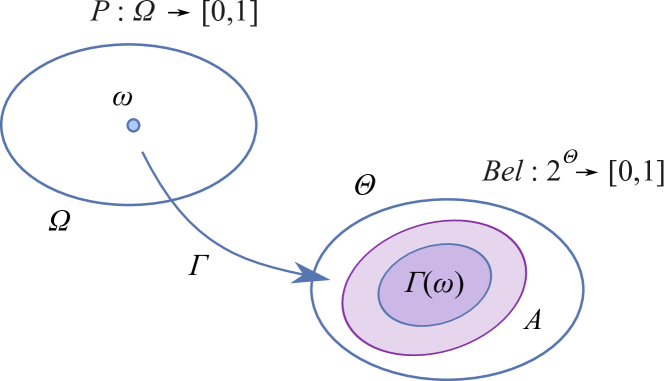
Figure 1: A probability measure $P$ on $\Omega$ induces via a multivalued mapping $\Gamma$ a belief function $Bel$ on $\Theta$ whose values are given in (4).

In Dempster’s original formulation, then, belief functions are objects induced by a source probability measure in a decision space for which we do not have a probability, as long as there exists a 1-many mapping between the two.

2.3.1 Belief and plausibility measures

A special class of lower and upper probabilities is provided by belief and plausibility measures. Namely, a basic probability assignment (BPA) [96] is a set function [65, 69] $m:2^{\Theta}\rightarrow[0,1]$ such that

$$m(\emptyset)=0,\quad\sum_{A\subset\Theta}m(A)=1.$$

Subsets of $\Theta$ whose mass values are non-zero are called focal elements of $m$. The belief function (BF) associated with a BPA $m:2^{\Theta}\rightarrow[0,1]$ is the set function $Bel:2^{\Theta}\rightarrow[0,1]$ defined as

$$Bel(A)=\sum_{B\subseteq A}m(B).$$ (5)

The corresponding plausibility function is

$$Pl(A)\doteq\sum_{B\cap A\neq\emptyset}m(B)\geq Bel(A).$$

Note that belief functions can also be equivalently defined in axiomatic terms [96].

Classical probability measures on $\Theta$ are a special case of belief functions (those assigning mass to singletons only), termed Bayesian belief functions. A BF is said to be consonant if its focal elements $A_{1},...,A_{m}$ are nested: $A_{1}\subset\cdots\subset A_{m}$, and corresponds to a possibility measure [70, 73, 96, 43].

2.3.2 Combination

In belief theory conditioning is replaced by the notion of (associative) combination of any number of belief functions.

The Dempster combination $Bel_{1}\oplus Bel_{2}$ of two belief functions on $\Theta$ is the unique BF there with as focal elements all the non-empty intersections of focal elements of $Bel_{1}$ and $Bel_{2}$, and basic probability assignment

$$m_{\oplus}(A)=\frac{m_{\cap}(A)}{1-m_{\cap}(\emptyset)},$$ (6)

where

$$m_{\cap}(A)=\sum_{B\cap C=A}m_{1}(B)m_{2}(C)$$ (7)

and $m_{i}$ is the BPA of the input belief function $Bel_{i}$.

Nevertheless, Dempster’s combination naturally induces a conditioning operator. Given a conditioning event $A\subset\Theta$, the ‘logical’ or categorical belief function $Bel_{A}$ such that $m(A)=1$ is combined via Dempster’s rule with the a-priori belief function $Bel$. The resulting BF $Bel\oplus Bel_{A}$ is the conditional belief function given $A$ a la Dempster, denoted by $Bel_{\oplus}(A|B)$.

Many alternative combination rules have since been defined [86, 119, 71, 67], often associated with a distinct approach to conditioning [64, 74, 108]. An exhaustive review of these proposals can be found in [43], Section 4.3.

Rather than normalising (as in Dempster’s rule) or reassigning the conflicting mass $m_{\cap}(\emptyset)$ to other non-empty subsets, Philippe Smets’s conjunctive rule leaves the conflicting mass with the empty set,

$$m_{\text{\text{$\scriptstyle{\cap}$⃝}}}(A)=\left\{\begin{array}[]{ll}m_{\cap}(A)&\emptyset\neq A\subseteq\Theta,\\ m_{\cap}(\emptyset)&A=\emptyset,\end{array}\right.$$ (8)

and thus is applicable to unnormalised belief functions [100].

In Dempster’s original random-set idea, consensus between two sources is expressed by the intersection of the supported events (7). When the union of the supported propositions is taken to represent such a consensus instead, we obtain what Smets called the disjunctive rule of combination,

$$m_{\text{\text{$\scriptstyle{\cup}$⃝}}}(A)=\sum_{B\cup C=A}m_{1}(B)m_{2}(C).$$ (9)

It is interesting to note that under disjunctive combination,

$$Bel_{1}$\scriptstyle{\cup}$⃝Bel_{2}(A)=Bel_{1}(A)\ast Bel_{2}(A),$$

i.e., the belief values of the input belief functions are simply multiplied.

2.3.3 Belief functions and other measures

Each belief function $Bel$ uniquely identifies a credal set [88]

$$\mathcal{P}[Bel]=\{P\in\mathcal{P}:P(A)\geq Bel(A)\}$$ (10)

(where $\mathcal{P}$ is the set of all probabilities one can define on $\Theta$), of which it is its lower envelope: $Bel(A)=\underline{P}(A)$. Belief functions are thus a special case of lower probabilities (Section 2.1). The corresponding plausibility measure is the upper probability of an event $A$: $Pl(A)=\overline{P}(A)$. The probability intervals resulting from Dempster’s updating of the credal set associated with a BF, however, are included in those resulting from Bayesian updating [88].

Belief functions are also infinitely monotone capacities [8, 107], and a special case of coherent lower previsions [114, 115]. Finally, every belief function specifies a unique probability box [75], i.e., a class of cumulative distribution functions delimited by two lower and upper bounds.

2.4 The geometry of uncertainty measures

Geometry has been proposed by this author and others as a unifying language for the field [42, 53, 54, 55, 58, 76, 77, 5, 85, 78, 116], possibly in conjunction with an algebraic view [51, 12, 23, 57, 16, 18, 38].

Indeed, uncertainty measures can be seen as points of a suitably complex geometric space, and there manipulated (e.g. combined, conditioned and so on) [13, 21, 43]. Much work has been focusing on the geometry of belief functions, which live in a convex space termed the belief space, which can be described both in terms of a simplex (a higher-dimensional triangle) and in terms of a recursive bundle structure [56, 45, 41, 52]. The analysis can be extended to Dempster’s rule of combination by introducing the notion of a conditional subspace and outlining a geometric construction for Dempster’s sum [49, 14]. The combinatorial properties of plausibility and commonality functions, as equivalent representations of the evidence carried by a belief function, have also been studied [22, 34]. The corresponding spaces are simplices which are congruent to the belief space.
Subsequent work extended the geometric approach to other uncertainty measures, focusing in particular on possibility measures (consonant belief functions) [32] and consistent belief functions [36, 48, 25], in terms of simplicial complexes [15]. Analyses of belief functions in terms credal sets have also been conducted [26, 1, 6].

The geometry of the relationship between measures of different kinds has also been extensively studied [50, 30, 17, 31], with particular attention to the problem of transforming a belief function into a classical probability measure [9, 112, 99] (see Section 3). One can distinguish between an affine family of probability transformations [20] (those which commute with affine combination in the belief space), and an epistemic family of transforms [19], formed by the relative belief and relative plausibility of singletons [28, 27, 37, 46, 33], which possess dual properties with respect to Dempster’s sum [24]. The problem of finding the possibility measure which best approximates a given belief function [2] can also be approached in geometric terms [29, 47, 39, 40]. In particular, approximations induced by classical Minkowski norms can be derived and compared with classical outer consonant approximations [72]. Minkowski consistent approximations of belief functions in both the mass and the belief space representations can also be derived [36].

The geometric approach to uncertainty can also be applied to the conditioning problem [89]. Conditional belief functions can be defined as those which minimise an appropriate distance between the original belief function and the ‘conditioning simplex’ associated with the conditioning event [44, 35].

Recent papers on this topic include [93, 95, 91].

3 Probability transform

3.1 Probability transforms of belief functions

The relation between belief and probability in the theory of evidence has been and continues to be an important subject of study[118, 87, 3, 4, 66, 68, 81]. A probability transform mapping belief functions to probability measures can be instrumental in addressing a number of issues: mitigating the inherently exponential complexity of belief calculus [3], making decisions via the probability distributions obtained in a utility theory framework [99] and obtaining pointwise estimates of quantities of interest from belief functions (e.g., the pose of an articulated object in computer vision: see [52], Chapter 8, or [54]).

As both belief and probability measures can be assimilated into points of a Cartesian space [43], the problem can (as mentioned) be posed in a geometric setting. Without loss of generality, we can define a probability transform as a mapping from the space of belief functions $\mathcal{B}$ on the domain of interest to the probability simplex $\mathcal{P}$ there,

$$\begin{array}[]{lllll}\mathcal{PT}&:&\mathcal{B}&\rightarrow&\mathcal{P},\\ &&Bel\in\mathcal{B}&\mapsto&\mathcal{PT}[Bel]\in\mathcal{P},\end{array}$$

such that an appropriate distance function or similarity measure $d$ from $Bel$ is minimised [59]:

$$\mathcal{PT}[Bel]=\arg\min_{P\in\mathcal{P}}d(Bel,P).$$ (11)

A minimal, sensible requirement is for the probability which results from the transform to be compatible with the upper and lower bounds that the original belief function $Bel$ enforces on the singletons only, rather than on all the focal sets. Thus, this does not require probability transforms to adhere to the upper–lower probability semantics of belief functions. As a matter of fact, some important transforms of this kind are not compatible with such semantics.

Many such transformations have been proposed, according to different criteria [92, 110, 4, 66, 68, 3]. In Smets’s transferable belief model [98, 104], in particular, decisions are made by resorting to the pignistic probability:

$$BetP[Bel](x)=\sum_{A\supseteq\{x\}}\frac{m(A)}{|A|},$$ (12)

which is the output of the pignistic transform.

An interesting approach to the problem seeks approximations which enjoy commutativity properties with respect to a specific combination rule, in particular Dempster’s sum [63, 62]. This is the case of the relative plausibility of singletons [112], the unique probability that, given a belief function $Bel$ with plausibility $Pl(A)=1-Bel(A^{c})$, assigns to each singleton its normalized plausibility:

$$\tilde{Pl}[Bel](x)=\frac{Pl(x)}{\sum_{y\in\Theta}Pl(y)}.$$ (13)

Its properties have been later analyzed by Cobb and Shenoy [9, 10]. Voorbraak proved that his (in our terminology) relative plausibility of singletons $\tilde{Pl}[Bel]$ is a perfect representative of $Bel$ when combined with other probabilities $P\in\mathcal{P}$ through Dempster’s rule $\oplus$:

$$\tilde{Pl}[Bel]\oplus P=Bel\oplus P\quad\forall P\in\mathcal{P}.$$ (14)

Dually, a relative belief transform $\tilde{Bel}:\mathcal{B}\rightarrow\mathcal{P}$, $Bel\mapsto\tilde{Bel}[Bel]$ mapping each belief function $Bel$ to the corresponding relative belief of singletons [24, 28, 80, 59],

$$\tilde{Bel}[Bel](x)=\frac{Bel(x)}{\sum_{y\in\Theta}Bel(y)},$$ (15)

can be defined. The notion of a relative belief transform (under the name of ‘normalised belief of singletons’) was first proposed by Daniel in [59]. Some analyses of the relative belief transform and its close relationship with the (relative) plausibility transform were presented in [24, 28].

3.2 Geometric approaches

Only a few authors have in the past posed the study of the connections between belief functions and probabilities in a geometric setting. In particular, Ha and Haddawy [79] proposed an ‘affine operator’, which can be considered a generalisation of both belief functions and interval probabilities, and can be used as a tool for constructing convex sets of probability distributions. In their work, uncertainty is modelled as sets of probabilities represented as ‘affine trees’, while actions (modifications of the uncertain state) are defined as tree manipulators. In a later publication [78], the same authors presented an interval generalisation of the probability cross-product operator, called the ‘convex-closure’ (cc) operator, analysed the properties of the cc operator relative to manipulations of sets of probabilities and presented interval versions of Bayesian propagation algorithms based on it. Probability intervals were represented there in a computationally efficient fashion by means of a data structure called a ‘pcc-tree’, in which branches are annotated with intervals, and nodes with convex sets of probabilities.

The intersection probability introduced in this paper is somewhat related to Ha’s cc operator, as it commutes (at least under certain conditions) with affine combination, and is therefore part of the affine family of Bayesian transforms of which Smets’s pignistic transform [102] is the foremost representative.

4 The intersection probability

When our uncertainty is described by imprecise probabilities, it may be desirable for some reasons to transform this knowledge into a classical unique probability. Such reasons include the need to take a unique optimal decision, the need to use classical probabilistic calculus (e.g., for efficiency), or more simply the will to obtain a unique probability from partial probabilistic information. Existing proposals are general in scope but rather complex, e.g., they imply solving a convex optimization problem.

4.1 Definition

There are clearly many ways of selecting a single measure to represent a collection of probability intervals (2). Note, however, that each of the intervals $[l(x),u(x)]$, $x\in\Theta$, carries the same weight within the system of constraints (2), as there is no reason for the different elements $x$ of the domain to be treated differently. It is then sensible to require that the desired representative probability should behave homogeneously in each element $x$ of the frame $\Theta$.

Mathematically, this translates into seeking a probability distribution $p:\Theta\rightarrow[0,1]$ such that

$$p(x)=l(x)+\alpha(u(x)-l(x))$$

for all the elements $x$ of $\Theta$, and some constant value $\alpha\in[0,1]$ (see Fig. 2). This value needs to be between 0 and 1 in order for the sought probability distribution $p$ to belong to the interval.

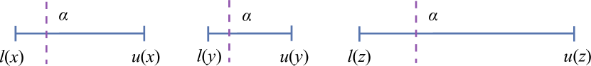
Figure 2: An illustration of the notion of the intersection probability for an interval probability system $(l,u)$ on $\Theta=\{x,y,z\}$ (2).

It is easy to see that there is indeed a unique solution to this problem. It suffices to enforce the normalisation constraint

$$\sum_{x}p(x)=\sum_{x}\Big{[}l(x)+\alpha(u(x)-l(x))\Big{]}=1$$

to understand that the unique value of $\alpha$ is given by

$$\alpha=\beta[(l,u)]\doteq\frac{1-\sum_{x\in\Theta}l(x)}{\sum_{x\in\Theta}\big{(}u(x)-l(x)\big{)}}.$$ (16)

Definition 1.

The intersection probability $p[(l,u)]:\Theta\rightarrow[0,1]$ associated with the interval probability system (2) is the probability distribution

$$p[(l,u)](x)=\beta[(l,u)]u(x)+(1-\beta[(l,u)])l(x),$$ (17)

with $\beta[(l,u)]$ given by (16).

The ratio $\beta[(l,u)]$ (16) measures the fraction of each interval $[l(x),u(x)]$ which we need to add to the lower bound $l(x)$ to obtain a valid probability function (adding up to one).

It is easy to see that when $(l,u)$ are a pair of belief/plausibility measures $(Bel,Pl)$, we can define the intersection probability for belief functions as well. Although originally defined by geometric means [20], the intersection probability is thus in fact ‘the’ rational probability transform for general interval probability systems.

Note that $p[(l,u)]$ can also be written as

$$p[(l,u)](x)=l(x)+\left(1-\sum_{x}l(x)\right)R[(l,u)](x),$$ (18)

where

$$R[(l,u)](x)\doteq\frac{u(x)-l(x)}{\sum_{y\in\Theta}(u(y)-l(y))}=\frac{\Delta(x)}{\sum_{y\in\Theta}\Delta(y)}.$$ (19)

Here $\Delta(x)$ measures the width of the probability interval for $x$, whereas $R[(l,u)]:\Theta\rightarrow[0,1]$ measures how much the uncertainty in the probability value of each singleton ‘weighs’ on the total width of the interval system (2). We thus term it the relative uncertainty of singletons. Therefore, we can say that $p[(l,u)]$ distributes the mass $(1-\sum_{x}l(x))$ to each singleton $x\in\Theta$ according to the relative uncertainty $R[(l,u)](x)$ it carries for the given interval.

Example 1.

Consider as an example an interval probability system on a domain $\Theta=\{x,y,z\}$ of size 3:

$$\begin{array}[]{lll}0.2\leq p(x)\leq 0.8,&0.4\leq p(y)\leq 1,&0.3\leq p(z)\leq 0.3.\end{array}$$ (20)

Notice that there is no uncertainty at all on the value of $p(z)=0.3$. The widths of the corresponding intervals are $\Delta(x)=0.6$, $\Delta(y)=0.6$, $\Delta(z)=0$ respectively. The relative uncertainty on each singleton (19) is therefore:

$$\begin{array}[]{lll}R[(l,u)](x)&=&\frac{\Delta(x)}{\sum_{w\in\Theta}\Delta(w)}=\frac{0.6}{1.2}=\frac{1}{2},\\ R[(l,u)](y)&=&\frac{1}{2},\\ R[(l,u)](z)&=&\frac{\Delta(z)}{\sum_{w\in\Theta}\Delta(w)}=\frac{0}{1.2}=0.\end{array}$$ (21)

Computing the intersection probability is then really easy. By Equation (16) the fraction of the uncertainty $u(x)-l(x)$ on $p(x)$ we need to add to the lower bound $l(x)$ to get an admissible, normalized probability is

$$\beta=\frac{1-0.2-0.4-0.3}{0.6+0.6}=\frac{0.1}{1.2}=\frac{1}{12}.$$

The intersection probability (18) has therefore values:

$$\begin{array}[]{c}p[(l,u)](x)=0.2+\frac{1}{12}0.6=0.25,\hskip 14.22636ptp[(l,u)](y)=0.4+\frac{1}{12}0.6=0.45,\\ \\ p[(l,u)](z)=0.3+\frac{1}{12}0=0.3.\end{array}$$

Notice that the fact of having a zero-width interval for one of the singletons does not pose a problem for the intersection probability, which falls as expected inside the probability interval for all the elements of the domain.

According to its interpretation of Equation (18), $p[(l,u)]$ is also the result of distributing the necessary mass $(1-\sum_{x}l(x))=1-0.2-0.4-0.3=0.1$ to each singleton in proportion to the relative uncertainty $R[(l,u)]$ (Equation (21)) of their intervals:

$$\begin{array}[]{c}p[(l,u)](x)=0.2+0.1\frac{1}{2}=0.25,\hskip 14.22636ptp[(l,u)](y)=0.4+0.1\frac{1}{2}=0.45,\\ \\ p[(l,u)](z)=0.3+0.1\cdot 0=0.3.\end{array}$$

4.2 Comparison with other interval representatives

It can be useful to briefly compare the proposed intersection probability with other possible representatives of an interval probability system (2).

4.2.1 Comparison with the center of mass of $P[(l,u)]$

The naive choice of picking the barycenter of each interval $[l(x),u(x)]$ to represent an interval probability system $(l,u)$, for instance, does not yield in general a valid probability function, for

$$\sum_{x\in\Theta}\left[l(x)+\frac{1}{2}(u(x)-l(x))\right]\neq 1.$$

This marks the difference with the case of belief functions, for which the pignistic function has a strong interpretation as barycenter of the associated credal set.

4.2.2 Comparison normalised lower and upper bounds

For the probability interval system (22) determined by a belief function,

$$(Bel,Pl)\doteq\big{\{}p\in\mathcal{P}:Bel(x)\leq p(x)\leq Pl(x),\forall x\in\Theta\big{\}},$$ (22)

the probabilities we obtain by normalizing lower $\tilde{l}(x)=l(x)/\sum_{y}l(y)$ or upper bound $\tilde{u}(x)=u(x)/\sum_{y}u(y)$ are not guaranteed to be consistent with the interval itself.

For instance, if there exists an element $x\in\Theta$ such that $Bel(x)=Pl(x)$ (the interval has width zero for that element) we have that

$$\tilde{Bel}(x)=\frac{m(x)}{\sum_{y}m(y)}>Pl(x),\quad\tilde{Pl}(x)=\frac{Pl(x)}{\sum_{y}Pl(y)}<Bel(x).$$

Therefore, both relative belief and plausibility of singletons fall outside the interval system (22). This holds for a general collection of probability intervals (2), again marking the contrast with the behavior of the intersection probability.

4.2.3 Comparison with Sudano’s proposal

In the belief functions framework, Sudano proposed in [106] the following four probability transforms:

$$\begin{array}[]{lll}PrPl[Bel](x)&\doteq&\displaystyle\sum_{A\supseteq\{x\}}m(A)\frac{Pl(x)}{\sum_{y\in A}Pl(y)},\end{array}$$ (24)

$$PrBel[Bel](x)\doteq\sum_{A\supseteq\{x\}}m(A)\frac{Bel(x)}{\sum_{y\in A}Bel(y)}=\sum_{A\supseteq\{x\}}m(A)\frac{m(x)}{\sum_{y\in A}m(y)},$$ (25)

$$PrNPl[Bel](x)\doteq\frac{1}{\Delta}\sum_{A\cap\{x\}\neq\emptyset}m(A)=\tilde{Pl}[Bel](x),$$ (26)

$$PraPl[Bel](x)\doteq Bel(x)+\epsilon\cdot Pl(x),\;\;\;\epsilon=\frac{1-\sum_{y\in\Theta}Bel(y)}{\sum_{y\in\Theta}Pl(y)}=\frac{1-k_{Bel}}{k_{Pl}},$$ (27)

where

$$k_{Bel}\doteq\sum_{x\in\Theta}Bel(x),\quad k_{Pl}\doteq\sum_{x\in\Theta}Pl(x).$$ (28)

The first two transformations are clearly inspired by the pignistic function (12). While in the latter case the mass $m(A)$ of each focal element is redistributed homogeneously to all its elements $x\in A$, $PrPl[Bel]$ (24) redistributes $m(A)$ proportionally to the relative plausibility of a singleton $x$ inside $A$. Similarly, $PrBel[Bel]$ (25) redistributes $m(A)$ proportionally to the relative belief of a singleton $x$ within $A$.

The fourth transformation (27), $PraPl[Bel]$, is more related to the case of probability intervals and to the intersection probability. By Equation (17),

$$\begin{array}[]{lll}p[Bel](x)&=&\displaystyle(1-\beta[Bel])\tilde{Bel}(x)k_{Bel}+\beta[Bel]\tilde{Pl}(x)k_{Pl},\end{array}$$ (29)

where

$$(1-\beta[Bel])k_{Bel}+\beta[Bel]k_{Pl}=\frac{k_{Pl}-1}{k_{Pl}-k_{Bel}}k_{Bel}+\frac{1-k_{Bel}}{k_{Pl}-k_{Bel}}k_{Pl}=1,$$

i.e., $p[Bel]$ lies on the line joining the relative plausibility $\tilde{Pl}$ and the relative belief $\tilde{Bel}$ of singletons. Here $\beta[Bel]$ is the value of (16) for a system of probability intervals associated with a belief function $Bel$, namely:

$$\beta[Bel]\doteq\frac{1-\sum_{x\in\Theta}Bel(x)}{\sum_{x\in\Theta}\big{(}Pl(x)-Bel(x)\big{)}}.$$ (30)

Just like the intersection probability (29) and the relative uncertainty of singletons [20], $PraPl[b]$ can also be expressed as an affine combination of relative belief and plausibility of singletons:

$$PraPl[Bel](x)=m(x)+\frac{1-k_{Bel}}{k_{Pl}}Pl(x)=k_{Bel}\tilde{Bel}(x)+(1-k_{Bel})\tilde{Pl}(x).$$ (31)

More to the point, as its definition only involves belief and plausibility values of singletons, it is more correct to think of $PraPl[b]$ as of a probability transformation of a probability interval system (rather than an approximation of a belief function)

$$PraPl[(l,u)]\doteq l(x)+\frac{1-\sum_{y}l(y)}{\sum_{y}u(y)}u(x)$$

just like the intersection probability.

However, it is easier to point out its weakness as a representative of probability intervals when put in the above form. Just like in the case of relative belief and plausibility of singletons, $PraPl[(l,u)]$ is not in general consistent with the original probability interval system $(l,u)$.
If there exists an element $x\in\Theta$ such that $l(x)=u(x)$ (the interval has width $\Delta(x)$ equal to zero for that element) we have that

$$\begin{array}[]{lll}PraPl[(l,u)](x)&=&\displaystyle l(x)+\frac{1-\sum_{y}l(y)}{\sum_{y}u(y)}u(x)=u(x)+\frac{1-\sum_{y}l(y)}{\sum_{y}u(y)}u(x)\\ &=&\displaystyle u(x)\cdot\frac{\sum_{y}u(y)+1-\sum_{y}l(y)}{\sum_{y}u(y)}>u(x)\end{array}$$

as $\frac{\sum_{y}u(y)+1-\sum_{y}l(y)}{\sum_{y}u(y)}>1$, and $PraPl[(l,u)]$ falls outside the interval.

Another fundamental objection against $PraPl[(l,u)]$ arises when we compare it to $p[(l,u)]$. While the latter adds to the lower bound $l(x)$ an equal fraction of the uncertainty $u(x)-l(x)$ for all singletons (18), $PraPl[(l,u)]$ adds to the lower bound $l(x)$ an equal fraction of the upper bound $u(x)$, effectively counting twice the evidence represented by the lower bound $l(x)$ (31).

In the case of belief functions, this amounts to adding to the mass value $m(x)$ of $x$ yet another fraction of $m(x)$ itself, instead of distributing only the remaining mass $Pl(x)-m(x)$ allowed to be assigned to $x$.

5 Geometric interpretation

Despite having being defined as a representative for systems of probability intervals, the intersection probability was first identified in the context of the geometric analysis of belief measures [21, 13, 56, 52]. As we briefly recall here, its very name derives from its geometry in the space of belief functions, or belief space [21, 49].

5.1 Geometry in the belief space

5.1.1 Belief space

Given a frame of discernment $\Theta$, a belief function $Bel:2^{\Theta}\rightarrow[0,1]$ is completely specified by its $N-2$ belief values $\{Bel(A),\emptyset\subsetneq A\subsetneq\Theta\}$, $N\doteq 2^{|\Theta|}$ (as $Bel(\emptyset)=0$, $Bel(\Theta)=1$ for all BFs), and can then be seen as a point of $\mathbb{R}^{N-2}$.

The belief space associated with $\Theta$ is the set of points $\mathcal{B}\subset\mathbb{R}^{N-2}$ which correspond to admissible belief functions [21]. This turns out to be the simplex determined by the convex closure of all the categorical belief functions $Bel_{A}$, namely

$$\mathcal{B}=Cl(Bel_{A},\;\emptyset\subsetneq A\subseteq\Theta),$$

($Bel_{\Theta}$ included). The faces of a simplex are all the simplices generated by a subset of its vertices. The set of all the Bayesian belief functions on $\Theta$, $\mathcal{P}=Cl(Bel_{x},x\in\Theta)$, is then a face of $\mathcal{B}$.

Plausibility functions, also determined by their $N-2$ values $\{Pl(A),\emptyset\subsetneq A\subsetneq\Theta\}$, can too be seen as points of $\mathbb{R}^{N-2}$. We call plausibility space [24, 22] the corresponding region $\mathcal{PL}$ of $\mathbb{R}^{N-2}$, again, a simplex [45].

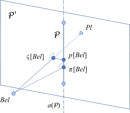
Figure 3: The geometry of the line $a(Bel,Pl)$ and the relative locations of $p[Bel]$, $\varsigma[Bel]$ and of the orthogonal projection $\pi[Bel]$ [20] for a frame of discernment of arbitrary size. Each belief function $Bel$ and the related plausibility function $Pl$ lie on opposite sides of the hyperplane $\mathcal{P}^{\prime}$ of all Bayesian pseudo belief functions [20], which divides the space $\mathbb{R}^{N-2}$ of all such functions into two halves. The line $a(Bel,Pl)$ connecting them always intersects $\mathcal{P}^{\prime}$, but not necessarily $a(\mathcal{P})$ (vertical line). This intersection $\varsigma[Bel]$ is naturally associated with a probability $p[Bel]$ (in general distinct from the orthogonal projection $\pi[Bel]$ of $Bel$ onto $\mathcal{P}$), having the same components in the base $\{Bel_{x},x\in\Theta\}$ of $a(\mathcal{P})$. $\mathcal{P}$ is a simplex (a segment in the figure) in $a(\mathcal{P})$: $\pi[Bel]$ and $p[Bel]$ are both ‘true’ probabilities.

5.1.2 Dual line

The intersection probability for a belief function $Bel$ can be shown to be the unique probability distribution determined by the intersection of the dual line joining a belief function $Bel$ and the related plausibility function $Pl$ with the region of Bayesian (pseudo) belief functions [20].

It can be shown that this dual line $a(Bel,Pl)$ is always orthogonal to $\mathcal{P}$, but it does not intersect the probabilistic subspace in general. It does always intersect, however, the region of Bayesian pseudo belief functions (or ‘normalised sum functions’) in a point

$$\varsigma[Bel]\doteq Bel+\beta[Bel](Pl-Bel)=a(Bel,Pl)\cap\mathcal{P}^{\prime}$$ (32)

(where $\mathcal{P}^{\prime}$ denotes the set of all Bayesian normalised sum functions in $\mathbb{R}^{N-2}$). $\varsigma[Bel]$ is a Bayesian pseudo BF but is not guaranteed to be a ‘proper’ Bayesian belief function.

But, of course, since $\sum_{x}m_{\varsigma[Bel]}(x)=1$, $\varsigma[Bel]$ is naturally associated with a Bayesian belief function assigning an equal amount of mass to each singleton and 0 to each $A:|A|>1$. Namely, we can define the probability measure

$$p[Bel]\doteq\sum_{x\in\Theta}m_{\varsigma[Bel]}(x)Bel_{x},$$ (33)

where $m_{\varsigma[Bel]}(x)$ is given by

$$m_{\varsigma[Bel]}(x)=m(x)+\beta[Bel]\sum_{A\supsetneq x}m(A).$$ (34)

This Bayesian BF $p[Bel]$ is nothing but the intersection probability associated with the probability interval system induced by $Bel$. The relative geometry of $\varsigma[Bel]$ and $p[Bel]$ with respect to the regions of Bayesian belief and normalised sum functions, respectively, is outlined in Fig. 3.

5.2 Justification for the name

The pseudo probability $\varsigma[Bel]$ (32) provides the justification for the name ‘intersection probability’. It turns out that $p[Bel]$ and $\varsigma[Bel]$ are equivalent when combined with a Bayesian belief function.

We first need to recall the following result [14].

Proposition 1.

The orthogonal sum $Bel\oplus(\alpha_{1}Bel_{1}+\alpha_{2}Bel_{2})$ of a belief function $Bel$ and any affine combination $\alpha_{1}Bel_{1}+\alpha_{2}Bel_{2}$, $\alpha_{1}+\alpha_{2}=1$ of other two belief functions $Bel_{1}$, $Bel_{2}$ on the same frame reads as

$$Bel\oplus(\alpha_{1}Bel_{1}+\alpha_{2}Bel_{2})=\gamma_{1}(Bel\oplus Bel_{1})+\gamma_{2}(Bel\oplus Bel_{2}),$$ (35)

where

$$\gamma_{i}=\frac{\alpha_{i}k(Bel,Bel_{i})}{\alpha_{1}k(Bel,Bel_{1})+\alpha_{2}k(Bel,Bel_{2})}$$

and $k(Bel,Bel_{i})$ is the normalisation factor of the orthogonal sum $Bel\oplus Bel_{i}$.

Similar results can be proven for both conjunctive and disjunctive rules.

Lemma 1.

Affine combination commutes with both conjunctive and disjunctive rules:

$$\begin{array}[]{l}Bel$\scriptstyle{\cap}$⃝(\alpha_{1}Bel_{1}+\alpha_{2}Bel_{2})=\alpha_{1}(Bel$\scriptstyle{\cap}$⃝Bel_{1})+\alpha_{2}(Bel$\scriptstyle{\cap}$⃝Bel_{2}),\\ Bel$\scriptstyle{\cup}$⃝(\alpha_{1}Bel_{1}+\alpha_{2}Bel_{2})=\alpha_{1}(Bel$\scriptstyle{\cup}$⃝Bel_{1})+\alpha_{2}(Bel$\scriptstyle{\cup}$⃝Bel_{2})\end{array}$$

whenever $\alpha_{1}+\alpha_{2}=1$.

Proof.

By definition (9), we have that $Bel$\scriptstyle{\cap}$⃝(\alpha_{1}Bel_{1}+\alpha_{2}Bel_{2})$ has basic probability assignment:

$$\begin{array}[]{lll}&&m_{Bel$\scriptstyle{\cap}$⃝(\alpha_{1}Bel_{1}+\alpha_{2}Bel_{2})}(A)\\ \\ &=&\displaystyle\sum_{B\cap C=A}m(B)m_{\alpha_{1}Bel_{1}+\alpha_{2}Bel_{2}}(C)\\ &=&\displaystyle\sum_{B\cap C=A}m(B)\big{(}\alpha_{1}m_{1}(C)+\alpha_{2}m_{2}(C)\big{)}\\ &=&\displaystyle\alpha_{1}\sum_{B\cap C=A}m(B)m_{1}(C)+\alpha_{2}\sum_{B\cap C=A}m(B)m_{2}(C)\\ \\ &=&\alpha_{1}m_{Bel$\scriptstyle{\cap}$⃝Bel_{1}}(A)+\alpha_{2}m_{Bel$\scriptstyle{\cap}$⃝Bel_{2}}(A).\end{array}$$

An analogous proof holds for (8). ∎

Theorem 1.

The combinations of $p[Bel]$ and $\varsigma[Bel]$ with any probability function $p\in\mathcal{P}$ coincide under both the Dempster (6) and conjunctive (9) rules:

$$\begin{array}[]{ccc}p[Bel]\oplus p=\varsigma[Bel]\oplus p,&p[Bel]\cap p=\varsigma[Bel]\cap p,&\forall p\in\mathcal{P}.\end{array}$$ (36)

Proof.

Let us define by

$$\mu(A)=\sum_{B\subseteq A}(-1)^{|A-B|}Pl(B)$$ (37)

the Moebius inverse of a plausibility function $Pl$ (see [22]). It can be proven that [34]:

$$\sum_{A\supseteq\{x\}}\mu(A)=m(x).$$ (38)

Now, applying Equation (35) to $\varsigma\oplus p$ yields

$$\begin{array}[]{lll}\varsigma\oplus p&=&\big{[}\beta[Bel]Pl+(1-\beta[Bel])Bel\big{]}\oplus p\\ \\ &=&\displaystyle\frac{\beta[Bel]k(p,Pl)Pl\oplus p+(1-\beta[Bel])k(p,Bel)Bel\oplus p}{\beta[Bel]k(p,Pl)+(1-\beta[Bel])k(p,Bel)}\end{array}$$ (39)

where

$$\begin{array}[]{llll}k(p,Pl)&=&\displaystyle\sum_{x\in\Theta}p(x)\left(\sum_{A\supseteq\{x\}}\mu(A)\right)&=\displaystyle\sum_{x\in\Theta}p(x)m(x),\\ \\ k(p,Bel)&=&\displaystyle\sum_{x\in\Theta}p(x)\left(\sum_{A\supseteq\{x\}}m(A)\right)&\displaystyle=\sum_{x\in\Theta}p(x)Pl(x).\end{array}$$

by Equation (38), and by the definition of the plausibility of singletons ($\sum_{A\supseteq\{x\}}m(A)=Pl(x)$). On the other hand, recalling Equation (29), we can write

$$p[Bel]=\beta[Bel]\bar{Pl}+(1-\beta[Bel])\bar{Bel}$$ (40)

where we call the quantities

$$\begin{array}[]{ccc}\displaystyle\bar{Pl}\doteq\sum_{x\in\Theta}Pl(x)Bel_{x}&&\displaystyle\bar{Bel}=\sum_{x\in\Theta}m(x)Bel_{x}\end{array}$$ (41)

plausibility of singletons and belief of singletons, respectively [27, 24, 33, 37], for sake of consistency of nomenclature. However, $\bar{Pl}$ is traditionally referred to as the contour function.

Therefore when we apply (35) to $p[Bel]\oplus p$, instead, we get (by Equation (40)):

$$\begin{array}[]{lll}p[Bel]\oplus p&=&\big{[}\beta[Bel]\bar{Pl}+(1-\beta[Bel])\bar{Bel}\big{]}\oplus p\\ \\ &=&\displaystyle\frac{\beta[Bel]k(p,\bar{Pl})\bar{Pl}\oplus p+(1-\beta[Bel])k(p,\bar{Bel})\bar{Bel}\oplus p}{\beta[Bel]k(p,\bar{Pl})+(1-\beta[Bel])k(p,\bar{Bel})}.\end{array}$$ (42)

By definition of Dempster’s combination (6):

$$\begin{array}[]{c}\displaystyle\bar{Pl}\oplus p=\frac{\displaystyle\sum_{x\in\Theta}Bel_{x}p(x)(Pl(x)+1-k_{Pl})}{k(p,\bar{Pl})},\\ \\ \displaystyle\bar{Bel}\oplus p=\frac{\displaystyle\sum_{x\in\Theta}Bel_{x}p(x)(m(x)+1-k_{Bel})}{k(p,\bar{Bel})}.\end{array}$$

Hence

$$\begin{array}[]{ll}\displaystyle k(p,\bar{Pl})\bar{Pl}\oplus p&\displaystyle=\sum_{x\in\Theta}Bel_{x}p(x)Pl(x)+(1-k_{Pl})\sum_{x\in\Theta}Bel_{x}p(x)\\ &=\displaystyle k(Bel,p)Bel\oplus p+(1-k_{Pl})p,\\ \\ \displaystyle k(p,\bar{Bel})\bar{Bel}\oplus p&\displaystyle=\sum_{x\in\Theta}Bel_{x}p(x)m(x)+(1-k_{Bel})\sum_{x\in\Theta}Bel_{x}p(x)\\ &=\displaystyle k(Pl,p)Pl\oplus p+(1-k_{Bel})p,\end{array}$$

as:

1. $\sum_{x\in\Theta}Bel_{x}p(x)=p$;

2. in the calculation of $Bel\oplus p$, each singleton $x$ is assigned mass

   $$p(x)\sum_{A\supseteq\{x\}}m(A)=p(x)Pl(x);$$

3. in the calculation of $Pl\oplus p$, each singleton $x$ is assigned mass

   $$p(x)\sum_{A\supseteq\{x\}}\mu(A)=p(x)m(x)$$

   (again by Equation (38)).

After replacing these expressions in the numerator of (42) we can notice that, as

$$\begin{array}[]{ccc}\displaystyle\beta[Bel]=\frac{1-k_{Bel}}{k_{Pl}-k_{Bel}},&&\displaystyle 1-\beta[Bel]=\frac{k_{Pl}-1}{k_{Pl}-k_{Bel}},\end{array}$$

the contributions of $p$ vanish, leaving expression (39) for $\varsigma\oplus p$.

As conjunctive rule and affine combination commute, and $k(Bel_{1},Bel_{2})=1$ for each pair of pseudo belief functions $Bel_{1},Bel_{2}$ under conjunctive combination, the proof holds for $$\scriptstyle{\cap}$⃝$ too. ∎

Even though $p[Bel]$ is not the actual intersection $\varsigma[Bel]$ of the line $a(Bel,Pl)$ with the region of pseudo probabilities in the belief space, it behaves exactly like it when aggregated to a probability distribution.

Notice that Theorem 1 is not a simple consequence of Voorbraak’s representation theorem [24]:

$$Bel\oplus p=\tilde{Pl}\oplus p.$$

It is indeed easy to prove that the relative plausibility of singletons of $\varsigma[Bel]$ is not $p[Bel]$. As $\varsigma[Bel](A)=Bel(A)+\beta[Bel][Pl-Bel](A)$ we have:

$$\begin{array}[]{lll}&&Pl_{\varsigma[Bel]}(x)\\ &=&\displaystyle 1-\varsigma[Bel](\{x\}^{c})=1-Bel(\{x\}^{c})-\beta[Bel]\left[Pl(\{x\}^{c})-Bel(\{x\}^{c})\right]\\ &=&\displaystyle Pl(x)-\beta[Bel]\left[1-Bel(x)-1+Pl(x)\right]\\ &=&Pl(x)-\beta[Bel]\left[Pl(x)-Bel(x)\right]\\ &=&\beta[Bel]Bel(x)+(1-\beta[Bel])Pl(x)=\beta[Bel]m(x)+(1-\beta[Bel])Pl(x).\end{array}$$

Its normalization factor is

$$\begin{array}[]{lll}\sum_{x}Pl_{\varsigma[Bel]}(x)&=&\displaystyle\sum_{x}Pl(x)-\beta[Bel]\left[\sum_{x}Pl(x)-\sum_{x}m(x)\right]\\ &=&\displaystyle\sum_{x}Pl(x)-1+\sum_{x}m(x).\end{array}$$

Clearly then

$$\tilde{Pl}_{\varsigma[Bel]}(x)=\frac{Pl_{\varsigma[Bel]}(x)}{\sum_{y}Pl_{\varsigma[Bel]}(y)}=\frac{\beta[Bel]m(x)+(1-\beta[Bel])Pl(x)}{\sum_{y}Pl(y)-1+\sum_{y}m(y)}$$

is different from $p[Bel](x)=\beta[Bel]Pl(x)+(1-\beta[Bel])m(x)$.

6 Credal rationale

Probability interval systems admit a credal representation, which for intervals associated with belief functions is also strictly related to the credal set $\mathcal{P}[Bel]$ of all consistent probabilities [31, 43].

By the definition (10) of $\mathcal{P}[Bel]$, it follows that the polytope of consistent probabilities can be decomposed into a number of component polytopes, namely

$$\mathcal{P}[Bel]=\bigcap_{i=1}^{n-1}\mathcal{P}^{i}[Bel],$$ (43)

where $\mathcal{P}^{i}[Bel]$ is the set of probabilities that satisfy the lower probability constraint for size-$i$ events,

$$\mathcal{P}^{i}[Bel]\doteq\Big{\{}P\in\mathcal{P}:P(A)\geq Bel(A),\forall A:|A|=i\Big{\}}.$$ (44)

Note that for $i=n$ the constraint is trivially satisfied by all probability measures $P$: $\mathcal{P}^{n}[Bel]=\mathcal{P}$.

6.1 Lower and upper simplices

A simple and elegant geometric description of interval probability systems can be provided if, instead of considering the polytopes (44), we focus on the credal sets

$$T^{i}[Bel]\doteq\Big{\{}P^{\prime}\in\mathcal{P}^{\prime}:P^{\prime}(A)\geq Bel(A),\forall A:|A|=i\Big{\}}.$$

Here $\mathcal{P}^{\prime}$ denotes the set of all pseudo-probability measures $P^{\prime}$ on $\Theta$, whose distribution $p^{\prime}:\Theta\rightarrow\mathbb{R}$ satisfy the normalisation constraint $\sum_{x\in\Theta}p^{\prime}(x)=1$ but not necessarily the non-negativity one – there may exist an element $x$ such that $p^{\prime}(x)<0$. In particular, we focus here on the set of pseudo-probability measures which satisfy the lower constraint on singletons,

$$T^{1}[Bel]\doteq\Big{\{}p^{\prime}\in\mathcal{P}^{\prime}:p^{\prime}(x)\geq Bel(x)\;\;\forall x\in\Theta\Big{\}},$$ (45)

and the set $T^{n-1}[Bel]$ of pseudo-probability measures which satisfy the analogous constraint on events of size $n-1$,

$$\begin{array}[]{lll}T^{n-1}[Bel]&\doteq&\Big{\{}P^{\prime}\in\mathcal{P}^{\prime}:P^{\prime}(A)\geq Bel(A)\;\;\forall A:|A|=n-1\Big{\}}\\ \\ &=&\Big{\{}P^{\prime}\in\mathcal{P}^{\prime}:P^{\prime}(\{x\}^{c})\geq Bel(\{x\}^{c})\;\;\forall x\in\Theta\Big{\}}\\ \\ &=&\Big{\{}p^{\prime}\in\mathcal{P}^{\prime}:p^{\prime}(x)\leq Pl(x)\;\;\forall x\in\Theta\Big{\}},\end{array}$$ (46)

i.e., the set of pseudo-probabilities which satisfy the upper constraint on singletons.

6.2 Simplicial form

The extension to pseudo-probabilities allows us to prove that the credal sets (45) and (46) have the form of simplices (see [31] and [43], Chapter 16).

Theorem 2.

The credal set $T^{1}[Bel]$, or lower simplex, can be written as

$$T^{1}[Bel]=Cl(t^{1}_{x}[Bel],x\in\Theta),$$ (47)

namely as the convex closure of the vertices

$$t^{1}_{x}[Bel]=\sum_{y\neq x}m(y)Bel_{y}+\left(1-\sum_{y\neq x}m(y)\right)Bel_{x}.$$ (48)

Dually, the upper simplex $T^{n-1}[Bel]$ reads as the convex closure

$$T^{n-1}[Bel]=Cl(t^{n-1}_{x}[Bel],x\in\Theta)$$ (49)

of the vertices

$$t^{n-1}_{x}[Bel]=\sum_{y\neq x}Pl(y)Bel_{y}+\left(1-\sum_{y\neq x}Pl(y)\right)Bel_{x}.$$ (50)

By (48), each vertex $t^{1}_{x}[Bel]$ of the lower simplex is a pseudo-probability that adds the total mass $1-k_{Bel}$ of non-singletons to that of the element $x$, leaving all the others unchanged:

$$m_{t^{1}_{x}[Bel]}(x)=m(x)+1-k_{Bel},\quad m_{t^{1}_{x}[Bel]}(y)=m(y)\;\forall y\neq x.$$

In fact, as $m_{t^{1}_{x}[Bel]}(z)\geq 0$ for all $z\in\Theta$ and for all $x\in\Theta$ (all $t^{1}_{x}[Bel]$ are actual probabilities), we have that

$$T^{1}[Bel]=\mathcal{P}^{1}[Bel],$$ (51)

and $T^{1}[Bel]$ is completely included in the probability simplex.

On the other hand, the vertices (50) of the upper simplex are not guaranteed to be valid probabilities.
Each vertex $t^{n-1}_{x}[Bel]$ assigns to each element of $\Theta$ different from $x$ its plausibility $Pl(y)=pl(y)$, while it subtracts from $Pl(x)$ the ‘excess’ plausibility $k_{Pl}-1$:

$$\begin{array}[]{llll}m_{t^{n-1}_{x}[Bel]}(x)&=&Pl(x)+(1-k_{Pl}),&\\ m_{t^{n-1}_{x}[Bel]}(y)&=&Pl(y)&\forall y\neq x.\end{array}$$

Now, as $1-k_{Pl}$ can be a negative quantity, $m_{t^{n-1}_{x}[Bel]}(x)$ can also be negative and $t^{n-1}_{x}[Bel]$ is not guaranteed to be a ‘true’ probability.

We will have confirmation of this fact in the example in Section 6.4.

6.3 Lower and upper simplices and probability intervals

By comparing (2), (45) and (46), it is clear that the credal set $\mathcal{P}[(l,u)]$ associated with a set of probability intervals $(l,u)$ is nothing but the intersection

$$\mathcal{P}[(l,u)]=T[l]\cap T[u]$$

of the lower and upper simplices (52) associated with its lower- and upper-bound constraints, respectively:

$$T[l]\doteq\Big{\{}p:p(x)\geq l(x)\;\forall x\in\Theta\Big{\}},\quad T[u]\doteq\Big{\{}p:p(x)\leq u(x)\;\;\forall x\in\Theta\Big{\}}.$$ (52)

In particular, when these lower and upper bounds are those enforced by a pair of belief and plausibility measures on the singleton elements of a frame of discernment, $l(x)=Bel(x)$ and $u(x)=Pl(x)$, we get

$$\mathcal{P}[(Bel,Pl)]=T^{1}[Bel]\cap T^{n-1}[Bel].$$

6.4 Ternary case

Let us consider the case of a frame of cardinality 3, $\Theta=\{x,y,z\}$, and a belief function $Bel$ with mass assignment

$$\begin{array}[]{ccc}m(x)=0.2,&m(y)=0.1,&m(z)=0.3,\\ \\ m(\{x,y\})=0.1,&m(\{y,z\})=0.2,&m(\Theta)=0.1.\end{array}$$ (53)

Figure 4 illustrates the geometry of the related credal set $\mathcal{P}[Bel]$ in the simplex, denoted by $Cl(P_{x},P_{y},P_{z})$, of all the probability measures on $\Theta$.

It is well known [7, 26] that the credal set associated with a belief function is a polytope whose vertices are associated with all possible permutations of singletons.

Proposition 2.

Given a belief function $Bel:2^{\Theta}\rightarrow[0,1]$, the simplex $\mathcal{P}[Bel]$ of the probability measures consistent with $Bel$ is the polytope

$$\mathcal{P}[Bel]=Cl(P^{\rho}[Bel]\;\forall\rho),$$

where $\rho$ is any permutation $\{x_{\rho(1)},\ldots,x_{\rho(n)}\}$ of the singletons of $\Theta$, and the vertex $P^{\rho}[Bel]$ is the Bayesian belief function such that

$$P^{\rho}[Bel](x_{\rho(i)})=\sum_{A\ni x_{\rho}(i),A\not\ni x_{\rho}(j)\;\forall j<i}m(A).$$ (54)

By Proposition 2, for the example belief function (53), $\mathcal{P}[Bel]$ has as vertices the probabilities $P^{\rho^{1}},P^{\rho^{2}},P^{\rho^{3}}$, $P^{\rho^{4}}$, $P^{\rho^{5}}[Bel]$ identified by purple squares in Fig. 4, namely

$$\begin{array}[]{llll}\rho^{1}=(x,y,z):&\quad P^{\rho^{1}}[Bel](x)=.4,&P^{\rho^{1}}[Bel](y)=.3,&P^{\rho^{1}}[Bel](z)=.3,\\ \rho^{2}=(x,z,y):&\quad P^{\rho^{2}}[Bel](x)=.4,&P^{\rho^{2}}[Bel](y)=.1,&P^{\rho^{2}}[Bel](z)=.5,\\ \rho^{3}=(y,x,z):&\quad P^{\rho^{3}}[Bel](x)=.2,&P^{\rho^{3}}[Bel](y)=.5,&P^{\rho^{3}}[Bel](z)=.3,\\ \rho^{4}=(z,x,y):&\quad P^{\rho^{4}}[Bel](x)=.3,&P^{\rho^{4}}[Bel](y)=.1,&P^{\rho^{4}}[Bel](z)=.6,\\ \rho^{5}=(z,y,x):&\quad P^{\rho^{5}}[Bel](x)=.2,&P^{\rho^{5}}[Bel](y)=.2,&P^{\rho^{5}}[Bel](z)=.6\end{array}$$ (55)

(as the permutations $(y,x,z)$ and $(y,z,x)$ yield the same probability distribution).

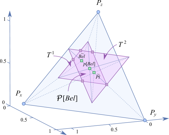
Figure 4: The polytope $\mathcal{P}[Bel]$ of probabilities consistent with the belief function $Bel$ (53) defined on $\{x,y,z\}$ is shown in a darker shade of purple, in the probability simplex $\mathcal{P}=Cl(P_{x},P_{y},P_{z})$ (shown in light blue). Its vertices (purple squares) are given in (55). The intersection probability, relative belief and relative plausibility of singletons (green squares) are the foci of the pairs of simplices $\{T^{1}[Bel],T^{2}[Bel]\}$, $\{T^{1}[Bel],\mathcal{P}\}$ and $\{\mathcal{P},T^{2}[Bel]\}$, respectively. In the ternary case, $T^{1}[Bel]$ and $T^{2}[Bel]$ (light purple) are regular triangles. Geometrically, their focus is the intersection of the lines joining their corresponding vertices (dashed lines for $\{T^{1}[Bel],\mathcal{P}\}$,$\{\mathcal{P},T^{2}[Bel]\}$; solid lines for $\{T^{1}[Bel],T^{2}[Bel]\}$).

We can notice a number of relevant facts:

1. As pointed out above, $\mathcal{P}[Bel]$ (the polygon delimited by the purple squares) is the intersection of the two triangles (two-dimensional simplices) $T^{1}[Bel]$ and $T^{2}[Bel]$.

2. The relative belief of singletons,

   $$\tilde{Bel}(x)=\frac{.2}{.6}=\frac{1}{3},\quad\tilde{Bel}(y)=\frac{.1}{.6}=\frac{1}{6},\quad\tilde{Bel}(z)=\frac{.3}{.6}=\frac{1}{2},$$

   is the intersection of the lines joining the corresponding vertices of the probability simplex $\mathcal{P}$ and the lower simplex $T^{1}[Bel]$.

3. The relative plausibility of singletons,

   $$\begin{array}[]{lll}\tilde{Pl}(x)&=&\displaystyle\frac{m(x)+m(\{x,y\})+m(\Theta)}{k_{Pl}-k_{Bel}}=\frac{.4}{.4+.5+.6}=\frac{4}{15},\\ \\ \tilde{Pl}(y)&=&\displaystyle\frac{.5}{.4+.5+.6}=\frac{1}{3},\quad\tilde{Pl}(z)=\frac{2}{5},\end{array}$$

   is the intersection of the lines joining the corresponding vertices of the probability simplex $\mathcal{P}$ and the upper simplex $T^{2}[Bel]$.

4. Finally, the intersection probability,

   $$\begin{array}[]{lll}p[Bel](x)&=&\displaystyle m(x)+\beta[Bel]\big{(}m(\{x,y\})+m(\Theta)\big{)}=.2+\frac{.4\ast 0.2}{1.5-0.4}=.27,\\ p[Bel](y)&=&\displaystyle.1+\frac{.4}{1.1}0.4=.245,\quad p[Bel](z)=.485,\end{array}$$

   is the unique intersection of the lines joining the corresponding vertices of the upper and lower simplices $T^{2}[Bel]$ and $T^{1}[Bel]$.

Although Fig. 4 suggests that $\tilde{Bel}$, $\tilde{Pl}$ and $p[Bel]$ might be consistent with $Bel$, this is a mere artefact of this ternary example, for it can be proved ([43], Chapter 12) that neither the relative belief of singletons nor the relative plausibility of singletons necessarily belongs to the credal set $\mathcal{P}[Bel]$. Indeed, the point here is that the epistemic transforms $\tilde{Bel}$, $\tilde{Pl}$, $p[Bel]$ are instead consistent with the interval probability system $\mathcal{P}[(Bel,Pl)]$ associated with the original belief function $Bel$:

$$\tilde{Bel},\tilde{Pl},p[Bel]\in\mathcal{P}[(Bel,Pl)]=T^{1}[Bel]\cap T^{n-1}[Bel].$$

Their geometric behaviour, as described by facts 2, 3 and 4, holds in the general case as well.

6.5 Focus of a pair of simplices

Definition 2.

Consider two simplices in $\mathbb{R}^{n-1}$, denoted by $S=Cl(s_{1},\ldots,s_{n})$ and $T=Cl(t_{1},\ldots,t_{n})$, with the same number of vertices. If there exists a permutation $\rho$ of $\{1,\ldots,n\}$ such that the intersection

$$\bigcap_{i=1}^{n}a(s_{i},t_{\rho(i)})$$ (56)

of the lines joining corresponding vertices of the two simplices exists and is unique, then $p=f(S,T)\doteq\bigcap_{i=1}^{n}a(s_{i},t_{\rho(i)})$ is termed the focus of the two simplices $S$ and $T$.

Not all pairs of simplices admit a focus. For instance, the pair of simplices (triangles) $S=Cl(s_{1}=[2,2]^{\prime},s_{2}=[5,2]^{\prime},s_{3}=[3,5]^{\prime})$ and $T=Cl(t_{1}=[3,1]^{\prime},t_{2}=[5,6]^{\prime},t_{3}=[2,6]^{\prime})$ in $\mathbb{R}^{2}$ does not admit a focus, as no matter what permutation of the order of the vertices we consider, the lines joining corresponding vertices do not intersect. Geometrically, all pairs of simplices admitting a focus can be constructed by considering all possible stars of lines, and all possible pairs of points on each line of each star as pairs of corresponding vertices of the two simplices.

Definition 3.

We call a focus special if the affine coordinates of $f(S,T)$ on the lines $a(s_{i},t_{\rho(i)})$ all coincide, namely $\exists\alpha\in\mathbb{R}$ such that

$$f(S,T)=\alpha s_{i}+(1-\alpha)t_{\rho(i)}\quad\forall i=1,\ldots,n.$$ (57)

Not all foci are special. As an example, the simplices $S=Cl(s_{1}=[-2,-2]^{\prime},s_{2}=[0,3]^{\prime},s_{3}=[1,0]^{\prime})$ and $T=Cl(t_{1}=[-1,0]^{\prime},t_{2}=[0,-1]^{\prime},t_{3}=[2,2]^{\prime})$ in $\mathbb{R}^{2}$ admit a focus, in particular for the permutation $\rho(1)=3,\rho(2)=2,\rho(3)=1$ (i.e., the lines $a(s_{1},t_{3})$, $a(s_{2},t_{2})$ and $a(s_{3},t_{1})$ intersect in $\mathbf{0}=[0,0]^{\prime}$). However, the focus $f(S,T)=[0,0]^{\prime}$ is not special, as its simplicial coordinates in the three lines are $\alpha=\frac{1}{2}$, $\alpha=\frac{1}{4}$ and $\alpha=\frac{1}{2}$, respectively.

On the other hand, given any pair of simplices in $\mathbb{R}^{n-1}$ $S=Cl(s_{1},\ldots,s_{n})$ and $T=Cl(t_{1},\ldots,t_{n})$, for any permutation $\rho$ of the indices there always exists a linear variety of points which have the same affine coordinates in both simplices,

$$\left\{p\in\mathbb{R}^{n-1}\Bigg{|}p=\sum_{i=1}^{n}\alpha_{i}s_{i}=\sum_{j=1}^{n}\alpha_{j}t_{\rho(j)},\;\sum_{i=1}^{n}\alpha_{i}=1.\right\}$$ (58)

Indeed, the conditions on the right-hand side of (58) amount to a linear system of $n$ equations in $n$ unknowns ($\alpha_{i}$, $i=1,\ldots,n$). Thus, there exists a linear variety of solutions to such a system, whose dimension depends on the rank of the matrix of constraints in (58).

It is rather easy to prove the following theorem.

Theorem 3.

Any special focus $f(S,T)$ of a pair of simplices $S,T$ has the same affine coordinates in both simplices, i.e.,

$$f(S,T)=\sum_{i=1}^{n}\alpha_{i}s_{i}=\sum_{j=1}^{n}\alpha_{j}t_{\rho(j)},\quad\sum_{i=1}^{n}\alpha_{i}=1,$$

where $\rho$ is the permutation of indices for which the intersection of the lines $a(s_{i},t_{\rho(i)})$, $i=1,\ldots,n$ exists.

Note that the affine coordinates $\{\alpha_{i},i\}$ associated with a focus can be negative, i.e., the focus may be located outside one or both simplices.

Notice also that the barycentre itself of a simplex is a special case of a focus. In fact, the centre of mass $b$ of a $d$-dimensional simplex $S$ is the intersection of the medians of $S$, i.e., the lines joining each vertex with the barycentre of the opposite (($d-1$)-dimensional) face (see Fig. 5). But those barycentres, for all ($d-1$)-dimensional faces, themselves constitute the vertices of a simplex $T$.

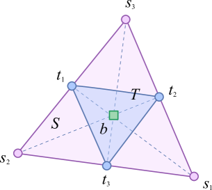
Figure 5: The barycentre of a simplex is itself a special case of a focus, as shown here for a two-dimensional example.

6.6 Intersection probability as a focus

Theorem 4.

For each belief function $Bel$, the intersection probability $p[Bel]$ has the same affine coordinates in the lower and upper simplices $T^{1}[Bel]$ and $T^{n-1}[Bel]$, respectively.

Theorem 5.

The intersection probability is the special focus of the pair of lower and upper simplices $\{T^{1}[Bel],T^{n-1}[Bel]\}$, with its affine coordinate on the corresponding intersecting lines equal to $\beta[Bel]$ (30).

The fraction $\alpha=\beta[Bel]$ of the width of the probability interval that generates the intersection probability can be read in the probability simplex as its coordinate on any of the lines determining the special focus of $\{T^{1}[Bel],T^{n-1}[Bel]\}$.

Similar results hold for the relative belief and relative plausibility of singletons, which are the (special) foci associated with the lower and upper simplices $T^{1}[Bel]$ and $T^{n-1}[Bel]$, the geometric incarnations of the lower and upper constraints on singletons. Those two simplices can also be interpreted as the sets of probabilities consistent with the plausibility and belief of singletons, respectively (see [43], Chapter 12).

Just as the pignistic function adheres to sensible rationality principles and, as a consequence, it has a clear geometrical interpretation as the centre of mass of the credal set associated with a belief function $Bel$, the intersection probability has an elegant geometric behaviour with respect to the credal set associated with an interval probability system, being the (special) focus of the related upper and lower simplices.

Now, selecting the special focus of two simplices representing two different constraints (i.e., the point with the same convex coordinates in the two simplices) means adopting the single probability distribution which satisfies both constraints in exactly the same way. If we assume homogeneous behaviour in the two sets of constraints $\{P(x)\geq Bel(x)\;\forall x\}$, $\{P(x)\leq Pl(x)\;\forall x\}$ as a rationality principle for the probability transformation of an interval probability system, then the intersection probability necessarily follows as the unique solution to the problem.

Another interesting results stems from the fact that the pignistic function and affine combination commute:

$$BetP[\alpha_{1}Bel_{1}+\alpha_{2}Bel_{2}]=\alpha_{1}BetP[Bel_{1}]+\alpha_{2}BetP[Bel_{2}]$$

whenever $\alpha_{1}+\alpha_{2}=1$.

Proposition 3.

[43] The intersection probability is the convex combination of the barycentres $t^{1}[Bel],t^{n-1}[Bel]$ of the lower and upper simplices $T^{1}[Bel],T^{n-1}[Bel]$ associated with a belief function $Bel$, with coefficient (30)

$$p[Bel]=\beta[Bel]t^{n-1}[Bel]+(1-\beta[Bel])t^{1}[Bel].$$

7 Relations with other probability transforms

In Section 4.2 we discussed how the intersection probability relates to alternative probability transforms for probability intervals, including Sudano’s proposals.

Since the intersection probability can also be interpreted (as we have seen) as a probability transform which applies to belief functions, it is quite natural to wonder how it relates to the two main classes of such transforms: the epistemic family and the affine family (see [43], Chapters 11 and 12).

7.1 Epistemic transforms

From (18) it follows that, for a belief function $Bel$,

$$p[Bel](x)=m(x)+(1-k_{Bel})\frac{Pl(x)-m(x)}{k_{Pl}-k_{Bel}},$$ (59)

which can be rewritten as:

$$p[Bel]=k_{Bel}\;\tilde{Bel}+(1-k_{Bel})R[Bel].$$ (60)

Since $k_{Bel}=\sum_{x\in\Theta}m(x)\leq 1$, (60) implies that the intersection probability $p[Bel]$ belongs to the segment linking the relative uncertainty of singletons $R[Bel]$ to the relative belief of singletons $\tilde{Bel}$. Its convex coordinate on this segment is the total mass of singletons $k_{Bel}$.

The relative plausibility function $\tilde{Pl}$ can also be written in terms of $\tilde{Bel}$ and $R[Bel]$ as, by definition (13),

$$\begin{array}[]{lll}R[Bel](x)&=&\displaystyle\frac{Pl(x)-m(x)}{k_{Pl}-k_{Bel}}=\frac{Pl(x)}{k_{Pl}-k_{Bel}}-\frac{m(x)}{k_{Pl}-k_{Bel}}\\ \\ &=&\displaystyle\tilde{Pl}(x)\frac{k_{Pl}}{k_{Pl}-k_{Bel}}-\tilde{Bel}(x)\frac{k_{Bel}}{k_{Pl}-k_{Bel}},\end{array}$$

since $\tilde{Pl}(x)=Pl(x)/k_{Pl}$ and $\tilde{Bel}(x)=m(x)/k_{Bel}$. Therefore,

$$\tilde{Pl}=\left(\frac{k_{Bel}}{k_{Pl}}\right)\tilde{Bel}+\left(1-\frac{k_{Bel}}{k_{Pl}}\right)R[Bel].$$ (61)

In summary, both the relative plausibility of singletons $\tilde{Pl}$ and the intersection probability $p[Bel]$ belong to the segment $Cl(R[Bel],\tilde{Bel})$ joining the relative belief $\tilde{Bel}$ and the relative uncertainty of singletons $R[Bel]$ (see Fig. 6). The convex coordinate of $\tilde{Pl}$ in $Cl(R[Bel],\tilde{Bel})$ (61) measures the ratio between the total mass and the total plausibility of the singletons, while that of $\tilde{Bel}$ measures the total mass of the singletons $k_{Bel}$. Since $k_{Pl}=\sum_{A\subset\Theta}m(A)|A|\geq 1$, we have that $k_{Bel}/k_{Pl}\leq k_{Bel}$: hence the relative plausibility function of singletons $\tilde{Pl}$ is closer to $R[Bel]$ than $p[Bel]$ is (Figure 6 again).

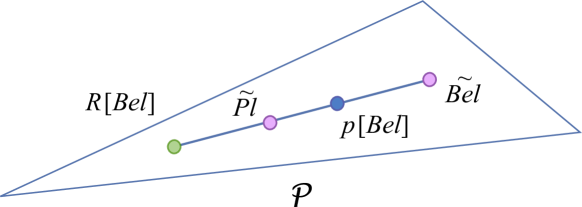
Figure 6: Location in the probability simplex $\mathcal{P}$ of the intersection probability $p[Bel]$ and the relative plausibility of singletons $\tilde{Pl}$ with respect to the relative uncertainty of singletons $R[Bel]$. They both lie on the segment joining $R[Bel]$ and the relative belief of singletons $\tilde{Bel}$, but $\tilde{Pl}$ is closer to $R[Bel]$ than $p[Bel]$ is.

Obviously, when $k_{Bel}=0$ (the relative belief of singletons $\tilde{Bel}$ does not exist, for $Bel$ assigns no mass to singletons), the remaining probability approximations coincide: $p[Bel]=\tilde{Pl}=R[Bel]$ by (59).

7.2 Pignistic function

To shed even more light on $p[Bel]$, and to get an alternative interpretation of the intersection probability, it is useful to compare $p[Bel]$ as expressed in (59) with the pignistic function,

$$BetP[Bel](x)\doteq\sum_{A\supseteq x}\frac{m(A)}{|A|}=m(x)+\sum_{A\supset x,A\neq x}\frac{m(A)}{|A|}.$$

In $BetP[Bel]$ the mass of each event $A$, $|A|>1$, is considered separately, and its mass $m(A)$ is shared equally among the elements of $A$. In $p[Bel]$, instead, it is the total mass $\sum_{|A|>1}m(A)=1-k_{Bel}$ of non-singleton focal sets which is considered, and this total mass is distributed proportionally to their non-Bayesian contribution to each element of $\Theta$.

Now, if $|A|>1$,

$$\beta[Bel_{A}]=\frac{\sum_{|B|>1}m(B)}{\sum_{|B|>1}m(B)|B|}=\frac{1}{|A|},$$

so that both $p[Bel](x)$ and $BetP[Bel](x)$ assume the form

$$m(x)+\sum_{A\supset x,A\neq x}m(A)\beta_{A},$$

where $\beta_{A}=\text{const}=\beta[Bel]$ for $p[Bel]$, while $\beta_{A}=\beta[Bel_{A}]$ in the case of the pignistic function.

Under what conditions do the intersection probability and pignistic function coincide? A sufficient condition can be easily given for a special class of belief functions.

Theorem 6.

The intersection probability and pignistic function coincide for a given belief function $Bel$ whenever the focal elements of $Bel$ have size 1 or $k$ only.

Proof.

The desired equality $p[Bel]=BetP[Bel]$ is equivalent to

$$m(x)+\sum_{A\supsetneq x}m(A)\beta[Bel]=m(x)+\sum_{A\supsetneq x}\frac{m(A)}{|A|},$$

which in turn reduces to

$$\sum_{A\supsetneq x}m(A)\beta[Bel]=\sum_{A\supsetneq x}\frac{m(A)}{|A|}.$$

If $\exists$ $k:m(A)=0$ for $|A|\neq k$, $|A|>1$, then $\beta[Bel]=1/k$ and the equality is satisfied. ∎

In particular, this is true when $Bel$ is 2-additive (its focal elements have cardinality $\leq 2$).

Example 1.

Let us briefly discuss these two interpretations of $p[Bel]$ in a simple example. Consider a ternary frame $\Theta=\{x,y,z\}$, and a belief function $Bel$ with BPA

$$\begin{array}[]{c}\begin{array}[]{ccc}m(x)=0.1,&m(y)=0,&m(z)=0.2,\end{array}\\ \begin{array}[]{cccc}m(\{x,y\})=0.3,&m(\{x,z\})=0.1,&m(\{y,z\})=0,&m(\Theta)=0.3.\end{array}\end{array}$$ (62)

The related basic plausibility assignment is, according to (37),

$$\begin{array}[]{c}\begin{array}[]{lll}\mu(x)&=&\displaystyle(-1)^{|x|+1}\sum_{B\supseteq\{x\}}m(B)\\ &=&\displaystyle m(x)+m(\{x,y\})+m(\{x,z\})+m(\Theta)=0.8,\end{array}\\ \\ \begin{array}[]{lllll}\mu(y)=0.6,&&\mu(z)=0.6,&&\mu(\{x,y\})=-0.6,\\ \\ \mu(\{x,z\})=-0.4,&&\mu(\{y,z\})=-0.3,&&\mu(\Theta)=0.3.\end{array}\end{array}$$

Figure 7 depicts the subsets of $\Theta$ with non-zero BPA (left) and BPlA (middle) induced by the belief function (62): dashed ellipses indicate a negative mass. The total mass that (62) accords to singletons is $k_{Bel}=0.1+0+0.2=0.3$. Thus, the line coordinate $\beta[Bel]$ of the intersection $\varsigma[Bel]$ of the line $a(Bel,Pl)$ with $\mathcal{P}^{\prime}$ is

$$\beta[Bel]=\frac{1-k_{Bel}}{m(\{x,y\})|\{x,y\}|+m(\{x,z\})|\{x,z\}|+m(\Theta)|\Theta|}=\frac{0.7}{1.7}.$$

By (34), the mass assignment of $\varsigma[Bel]$ is therefore

$$\begin{array}[]{l}\displaystyle m_{\varsigma[Bel]}(x)=m(x)+\beta[Bel](\mu(x)-m(x))=0.1+0.7\cdot\frac{0.7}{1.7}=0.388,\\ \\ \displaystyle m_{\varsigma[Bel]}(y)=0+0.6\cdot\frac{0.7}{1.7}=0.247,\;\;\;\;\;\;\;\;\;m_{\varsigma[Bel]}(z)=0.2+0.4\cdot\frac{0.7}{1.7}=0.365,\\ \\ \displaystyle m_{\varsigma[Bel]}(\{x,y\})=0.3-0.9\cdot\frac{0.7}{1.7}=-0.071,\\ \\ \displaystyle m_{\varsigma[Bel]}(\{x,z\})=0.1-0.5\cdot\frac{0.7}{1.7}=-0.106,\\ \\ \displaystyle m_{\varsigma[Bel]}(\{y,z\})=0-0.3\cdot\frac{0.7}{1.7}=-0.123,\;\;\;\;m_{\varsigma[Bel]}(\Theta)=0.3+0\cdot\frac{0.7}{1.7}=0.3.\end{array}$$

We can verify that all singleton masses are indeed non-negative and add up to one, while the masses of the non-singleton events add up to zero,

$$-0.071-0.106-0.123+0.3=0,$$

confirming that $\varsigma[Bel]$ is a Bayesian normalised sum function (pseudo belief function). Its mass assignment has signs which are still described by Fig. 7 (middle) although, as $m_{\varsigma[Bel]}$ is a weighted average of $m$ and $\mu$, its mass values are closer to zero.

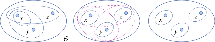
Figure 7: Signs of non-zero masses assigned to events by the functions discussed in Example 1. Left: BPA of the belief function (62), with five focal elements. Middle: the associated BPlA assigns positive masses (solid ellipses) to all events of size 1 and 3, and negative ones (dashed ellipses) to all events of size 2. This is the case for the mass assignment associated with $\varsigma$ (34) too. Right: the intersection probability $p[Bel]$ (33) retains, among the latter, only the masses assigned to singletons.

In order to compare $\varsigma[Bel]$ with the intersection probability, we need to recall (59): the non-Bayesian contributions of $x,y,z$ are, respectively,

$$\begin{array}[]{lll}Pl(x)-m(x)&=&m(\Theta)+m(\{x,y\})+m(\{x,z\})=0.7,\\ Pl(y)-m(y)&=&m(\{x,y\})+m(\Theta)=0.6,\\ Pl(z)-m(z)&=&m(\{x,z\})+m(\Theta)=0.4,\end{array}$$

so that the relative uncertainty of singletons is

$$R(x)=0.7/1.7,\quad R(y)=0.6/1.7,\quad R(z)=0.4/1.7.$$

For each singleton $\theta$, the value of the intersection probability results from adding to the original BPA $m(\theta)$ a share of the mass of the non-singleton events $1-k_{Bel}=0.7$ proportional to the value of $R(\theta)$ (see Fig. 7, right):

$$\begin{array}[]{lllll}p[Bel](x)&=&m(x)+(1-k_{Bel})R(x)=0.1+0.7*0.7/1.7&=&0.388,\\ p[Bel](y)&=&m(y)+(1-k_{Bel})R(y)=0+0.7*0.6/1.7&=&0.247,\\ p[Bel](z)&=&m(z)+(1-k_{Bel})R(z)=0.2+0.7*0.4/1.7&=&0.365.\end{array}$$

We can see that $p[Bel]$ coincides with the restriction of $\varsigma[Bel]$ to singletons.

Equivalently, $\beta[Bel]$ measures the share of $Pl(x)-m(x)$ assigned to each element of the frame of discernment:

$$\begin{array}[]{lllll}p[Bel](x)&=&m(x)+\beta[Bel](Pl(x)-m(x))&=&0.1+0.7/1.7*0.7,\\ p[Bel](y)&=&m(y)+\beta[Bel](Pl(y)-m(y))&=&0+0.7/1.7*0.6,\\ p[Bel](z)&=&m(z)+\beta[Bel](Pl(z)-m(z))&=&0.2+0.7/1.7*0.4.\end{array}$$

8 Operators

To complete our analysis, it can be useful to understand the way the intersection probability relates to two major (geometric) operators in the space of belief functions: affine combination and convex closure.

8.1 Affine combination

We have seen in Section 7 that $p[Bel]$ and $BetP[Bel]$ are closely related probability transforms, linked by the role of the quantity $\beta[Bel]$. It is natural to wonder whether $p[Bel]$ exhibits a similar behaviour with respect to the convex closure operator (see [43], Chapter 4). Indeed, although the situation is a little more complex in this second case, $p[Bel]$ turns also out to be related to $Cl(.)$ in a rather elegant way.

Let us introduce the notation $\beta[Bel_{i}]=N_{i}/D_{i}$.

Theorem 7.

Given two arbitrary belief functions $Bel_{1},Bel_{2}$ defined on the same frame of discernment, the intersection probability of their affine combination $\alpha_{1}\;Bel_{1}$ $+\;\alpha_{2}\;Bel_{2}$ is, for any $\alpha_{1}\in[0,1]$, $\alpha_{2}=1-\alpha_{1}$,

$$\begin{array}[]{lll}p[\alpha_{1}\;Bel_{1}+\alpha_{2}\;Bel_{2}]&=&\displaystyle\widehat{\alpha_{1}D_{1}}\big{(}\alpha_{1}p[Bel_{1}]+\alpha_{2}T[Bel_{1},Bel_{2}]\big{)}\\ \\ &&\displaystyle+\widehat{\alpha_{2}D_{2}}\big{(}\alpha_{1}T[Bel_{1},Bel_{2}])+\alpha_{2}p[Bel_{2}]\big{)},\end{array}$$ (63)

where $\widehat{\alpha_{i}D_{i}}=\frac{\alpha_{i}D_{i}}{\alpha_{1}D_{1}+\alpha_{2}D_{2}}$, $T[Bel_{1},Bel_{2}]$ is the probability with values

$$T[Bel_{1},Bel_{2}](x)\doteq\hat{D}_{1}p[Bel_{2},Bel_{1}]+\hat{D}_{2}p[Bel_{1},Bel_{2}],$$ (64)

with $\hat{D}_{i}\doteq\frac{D_{i}}{D_{1}+D_{2}}$, and

$$\begin{array}[]{c}p[Bel_{2},Bel_{1}](x)\doteq m_{2}(x)+\beta[Bel_{1}]\big{(}Pl_{2}(x)-m_{2}(x)\big{)},\\ \\ p[Bel_{1},Bel_{2}](x)\doteq m_{1}(x)+\beta[Bel_{2}]\big{(}Pl_{1}(x)-m_{1}(x)\big{)}.\end{array}$$ (65)

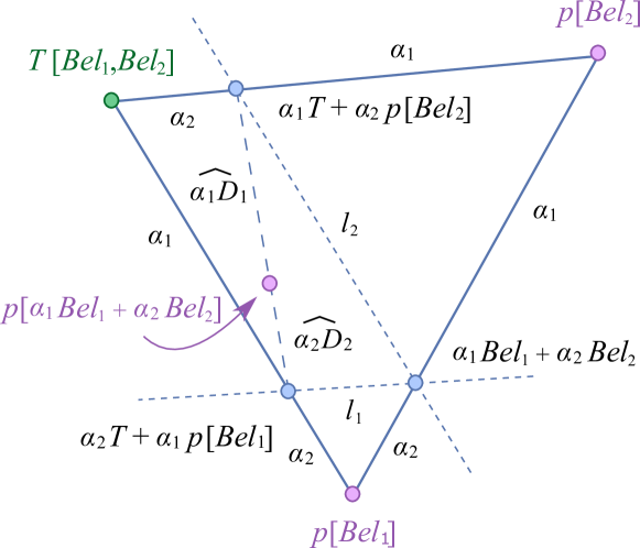
Figure 8: Behaviour of the intersection probability $p[Bel]$ under affine combination. $\alpha_{2}T+\alpha_{1}p[Bel_{1}]$ and $\alpha_{1}T+\alpha_{2}p[Bel_{2}]$ lie in inverted locations on the segments joining $T[Bel_{1},Bel_{2}]$ and $p[Bel_{1}]$, $p[Bel_{2}]$, respectively: $\alpha_{i}p[Bel_{i}]+\alpha_{j}T$ is the intersection of the line $Cl(T,p[Bel_{i}])$ with the line parallel to $Cl(T,p[Bel_{j}])$ passing through $\alpha_{1}p[Bel_{1}]+\alpha_{2}p[Bel_{2}]$. The quantity $p[\alpha_{1}Bel_{1}+\alpha_{2}Bel_{2}]$ is, finally, the point of the segment joining them with convex coordinate $\widehat{\alpha_{i}D_{i}}$.

Geometrically, $p[\alpha_{1}\;Bel_{1}+\alpha_{2}\;Bel_{2}]$ can be constructed as in Fig. 8 as a point of the simplex $Cl(T[Bel_{1},Bel_{2}],p[Bel_{1}],p[Bel_{2}])$. The point

$$\alpha_{1}T[Bel_{1},Bel_{2}]+\alpha_{2}p[Bel_{2}]$$

is the intersection of the segment $Cl(T,p[Bel_{2}])$ with the line $l_{2}$ passing through $\alpha_{1}p[Bel_{1}]+\alpha_{2}p[Bel_{2}]$ and parallel to $Cl(T,p[Bel_{1}])$. Dually, the point

$$\alpha_{2}T[Bel_{1},Bel_{2}]+\alpha_{1}p[Bel_{1}]$$

is the intersection of the segment $Cl(T,p[Bel_{1}])$ with the line $l_{1}$ passing through $\alpha_{1}p[Bel_{1}]+\alpha_{2}p[Bel_{2}]$ and parallel to $Cl(T,p[Bel_{2}])$. Finally, $p[\alpha_{1}Bel_{1}+\alpha_{2}Bel_{2}]$ is the point of the segment

$$Cl(\alpha_{1}T+\alpha_{2}p[Bel_{2}],\alpha_{2}T+\alpha_{1}p[Bel_{1}])$$

with convex coordinate $\widehat{\alpha_{1}D_{1}}$ (or, equivalently, $\widehat{\alpha_{2}D_{2}}$).

8.1.1 Location of $T[Bel_{1},Bel_{2}]$ in the binary case

As an example, let us consider the location of $T[Bel_{1},Bel_{2}]$ in the binary belief space $\mathcal{B}_{2}$ (Fig. 9), where

$$\beta[Bel_{1}]=\beta[Bel_{2}]=\frac{m_{i}(\Theta)}{2m_{i}(\Theta)}=\frac{1}{2}\quad\forall Bel_{1},Bel_{2}\in\mathcal{B}_{2},$$

and $p[Bel]$ always commutes with the convex closure operator. Accordingly,

$$\begin{array}[]{lll}\displaystyle T[Bel_{1},Bel_{2}](x)&=&\displaystyle\frac{m_{1}(\Theta)}{m_{1}(\Theta)+m_{2}(\Theta)}\left[m_{2}(x)+\frac{m_{2}(\Theta)}{2}\right]\\ \\ &&\displaystyle+\frac{m_{2}(\Theta)}{m_{1}(\Theta)+m_{2}(\Theta)}\left[m_{1}(x)+\frac{m_{1}(\Theta)}{2}\right]\\ \\ &=&\displaystyle\frac{m_{1}(\Theta)}{m_{1}(\Theta)+m_{2}(\Theta)}p[Bel_{2}]+\frac{m_{2}(\Theta)}{m_{1}(\Theta)+m_{2}(\Theta)}p[Bel_{1}].\end{array}$$

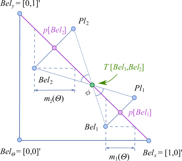
Figure 9: Location of the probability function $T[Bel_{1},Bel_{2}]$ in the binary belief space $\mathcal{B}_{2}$.

Looking at Figure 9, simple trigonometric considerations show that the segment defined by $Cl(p[Bel_{i}],T[Bel_{1},Bel_{2}])$ has length $m_{i}(\Theta)/(\sqrt{2}\tan{\phi})$, where $\phi$ is the angle between the segments $Cl(Bel_{i},T)$ and $Cl(p[Bel_{i}],T)$. $T[Bel_{1},Bel_{2}]$ is then the unique point of $\mathcal{P}$ such that the angles $\widehat{Bel_{1}Tp[Bel_{1}]}$ and $\widehat{Bel_{2}Tp[Bel_{2}]}$ coincide, i.e., $T$ is the intersection of $\mathcal{P}$ with the line passing through $Bel_{i}$ and the reflection of $Bel_{j}$ through $\mathcal{P}$. As this reflection (in $\mathcal{B}_{2}$) is nothing but $Pl_{j}$,

$$T[Bel_{1},Bel_{2}]=Cl(Bel_{1},Pl_{2})\cap\mathcal{P}=Cl(Bel_{2},Pl_{1})\cap\mathcal{P}.$$

8.2 Convex closure

Although the intersection probability does not commute with affine combination (Theorem 7), $p[Bel]$ can still be assimilated into the orthogonal projection and the pignistic function. Theorem 8 states the conditions under which $p[Bel]$ and convex closure ($Cl$) commute.

Theorem 8.

The intersection probability and convex closure commute iff

$$T[Bel_{1},Bel_{2}]=\hat{D}_{1}p[Bel_{2}]+\hat{D}_{2}p[Bel_{1}]$$

or, equivalently, either $\beta[Bel_{1}]=\beta[Bel_{2}]$ or $R[Bel_{1}]=R[Bel_{2}]$.

Geometrically, only when the two lines $l_{1},l_{2}$ in Fig. 8 are parallel to the affine space $a(p[Bel_{1}],p[Bel_{2}])$ (i.e., $T[Bel_{1},Bel_{2}]\in Cl(p[Bel_{1}],p[Bel_{2}])$; compare the above) does the desired quantity $p[\alpha_{1}Bel_{1}+\alpha_{2}Bel_{2}]$ belong to the line segment $Cl(p[Bel_{1}],p[Bel_{2}])$ (i.e., it is also a convex combination of $p[Bel_{1}]$ and $p[Bel_{2}]$).

Theorem 8 reflects the two complementary interpretations of $p[Bel]$ we gave in terms of $\beta[Bel]$ and $R[Bel]$:

$$\begin{array}[]{l}p[Bel]=m(x)+(1-k_{Bel})R[Bel](x),\\ \\ p[Bel]=m(x)+\beta[Bel](Pl(x)-m(x)).\end{array}$$

If $\beta[Bel_{1}]=\beta[Bel_{2}]$, both belief functions assign to each singleton the same share of their non-Bayesian contribution. If $R[Bel_{1}]=R[Bel_{2}]$, the non-Bayesian mass $1-k_{Bel}$ is distributed in the same way to the elements of $\Theta$.

A sufficient condition for the commutativity of $p[.]$ and $Cl(.)$ can be obtained via the following decomposition of $\beta[Bel]$:

$$\begin{array}[]{l}\displaystyle\beta[Bel]=\frac{\sum_{|B|>1}m(B)}{\sum_{|B|>1}m(B)|B|}=\frac{\sum_{k=2}^{n}\sum_{|B|=k}m(B)}{\sum_{k=2}^{n}k\cdot\sum_{|B|=k}m(B)}=\frac{\sigma_{2}+\cdots+\sigma_{n}}{2\sigma_{2}+\cdots+n\sigma_{n}},\end{array}$$ (66)

where $\sigma_{k}\doteq\sum_{|B|=k}m(B)$.

Theorem 9.

If the ratio between the total masses of focal elements of different cardinality is the same for all the belief functions involved, namely

$$\begin{array}[]{cccc}\displaystyle\frac{\sigma_{1}^{l}}{\sigma_{1}^{m}}=\frac{\sigma_{2}^{l}}{\sigma_{2}^{m}}&\quad\forall l,m\geq 2&\text{s.t.}&\sigma_{1}^{m},\sigma_{2}^{m}\neq 0,\end{array}$$ (67)

then the intersection probability (considered as an operator mapping belief functions to probabilities) and convex combination commute.

9 Conclusions

The intersection probability possesses a simple credal interpretation in the probability simplex (Section 6), as it can be linked to a pair of credal sets, thus in turn extending the classical interpretation of the pignistic transformation as the barycentre of the polygon of consistent probabilities.

Just like $\mathcal{P}[Bel]$ is the credal set associated with a belief function $Bel$, the upper and lower simplices geometrically embody the probability interval associated with $Bel$:

$$\mathcal{P}[(Bel,Pl)]=\Big{\{}p\in\mathcal{P}:Bel(x)\leq p(x)\leq Pl(x),\forall x\in\Theta\Big{\}}.$$

The intersection probability turns out to be the focus to the pair $\{T^{1}[Bel],T^{n-1}[Bel]\}$ of lower and upper simplices:

$$f(T^{1}[Bel],T^{n-1}[Bel])=p[Bel].$$ (68)

Its coordinates as foci encode major features of the underlying belief function, in particular the fraction $\beta$ of the related probability interval which yields the intersection probability.

This credal interpretation hints at the possible formulation of a decision making framework for probability intervals analogous to Smets’s transferable belief model (TBM) [101]. We can think of the TBM as a pair $\{\mathcal{P}[Bel],BetP[Bel]\}$ formed by a credal set linked to each belief function $Bel$ (in this case the polytope of consistent probabilities) and a probability transformation (the pignistic function). As the barycentre of a simplex is a special case of a focus, the pignistic transformation is just another probability transformation induced by the focus of two simplices.

The results in this paper therefore suggest a similar framework

$$\Big{\{}\big{\{}T^{1}[Bel],T^{n-1}[Bel]\big{\}},p[Bel]\Big{\}},$$

in which interval constraints on probability distributions on $\mathcal{P}$ are represented by a similar pair, formed by the above pair of simplices and by the probability transformation identified by their focus. Decisions are then made based on the appropriate focus probability, i.e., the intersection probability.

In the TBM [101], disjunctive/conjunctive combination rules are applied to belief functions to update or revise our state of belief according to new evidence. The formulation of a similar alternative frameworks for interval probability systems would then require us to design specific evidence elicitation/revision operators for them. This elicits a number of questions: how can we design such operator(s)? How are they related to combination rules for belief functions in the case of probability intervals induced by belief functions?

We will further explore the betting interpretation of the intersection probability in the near future.

Appendix

Proof of Theorem 2

Lemma 2.

The points $\{t_{x}^{1}[Bel],x\in\Theta\}$ are affinely independent.

Proof.

Let us suppose, contrary to the thesis, that there exists an affine decomposition of one of the points, say $t_{x}[Bel]$, in terms of the others:

$$t_{x}^{1}[Bel]=\sum_{z\neq x}\alpha_{z}t_{z}^{1}[Bel],\quad\alpha_{z}\geq 0\;\forall z\neq x,\;\sum_{z\neq x}\alpha_{z}=1.$$

But then we would have, by the definition of $t_{z}^{1}[Bel]$,

$$\begin{array}[]{lll}t_{x}^{1}[Bel]&=&\displaystyle\sum_{z\neq x}\alpha_{z}t_{z}^{1}[Bel]\\ &=&\displaystyle\sum_{z\neq x}\alpha_{z}\left(\sum_{y\neq z}m(y)Bel_{y}\right)+\sum_{z\neq x}\alpha_{z}\big{(}m(z)+1-k_{Bel}\big{)}Bel_{z}\\ \\ &=&\displaystyle m(x)Bel_{x}\sum_{z\neq x}\alpha_{z}+\sum_{z\neq x}Bel_{z}m(z)(1-\alpha_{z})\end{array}$$

$$\begin{array}[]{lll}&&+\displaystyle\sum_{z\neq x}\alpha_{z}m(z)Bel_{z}+(1-k_{Bel})\sum_{z\neq x}\alpha_{z}Bel_{z}\\ \\ &=&\displaystyle\sum_{z\neq x}m(z)Bel_{z}+m(x)Bel_{x}+(1-k_{Bel})\sum_{z\neq x}\alpha_{z}Bel_{z}.\end{array}$$

The latter is equal to (48)

$$t_{x}^{1}[Bel]=\sum_{z\neq x}m(z)Bel_{z}+(m(x)+1-k_{Bel})Bel_{x}$$

if and only if $\sum_{z\neq x}\alpha_{z}Bel_{z}=Bel_{x}.$ But this is impossible, as the categorical probabilities $Bel_{x}$ are trivially affinely independent. ∎

Proof of Theorem 3

Suppose that $p$ is a special focus of $S$ and $T$, namely $\exists\alpha\in\mathbb{R}$ such that

$$p=\alpha s_{i}+(1-\alpha)t_{\rho(i)}\quad\forall i=1,\ldots,n,$$

for some permutation $\rho$ of $\{1,\ldots,n\}$. Then, necessarily,

$$t_{\rho(i)}=\frac{1}{1-\alpha}[p-\alpha s_{i}]\quad\forall i=1,\ldots,n.$$

If $p$ has coordinates $\{\alpha_{i},i=1,\ldots,n\}$ in $T$, $p=\sum_{i=1}^{n}\alpha_{i}t_{\rho(i)}$, it follows that

$$\begin{array}[]{lll}p&=&\displaystyle\sum_{i=1}^{n}\alpha_{i}t_{\rho(i)}=\frac{1}{1-\alpha}\sum_{i}\alpha_{i}\big{[}p-\alpha s_{i}\big{]}\\ \\ &=&\displaystyle\frac{1}{1-\alpha}\left[p\sum_{i}\alpha_{i}-\alpha\sum_{i}\alpha_{i}s_{i}\right]=\frac{1}{1-\alpha}\left[p-\alpha\sum_{i}\alpha_{i}s_{i}\right].\end{array}$$

The latter implies that $p=\sum_{i}\alpha_{i}s_{i}$, i.e., $p$ has the same simplicial coordinates in $S$ and $T$.

Proof of Theorem 4

The common simplicial coordinates of $p[Bel]$ in $T^{1}[Bel]$ and $T^{n-1}[Bel]$ turn out to be the values of the relative uncertainty function (19) for $Bel$,

$$R[Bel](x)=\frac{Pl(x)-m(x)}{k_{Pl}-k_{Bel}}.$$ (69)

Recalling the expression (48) for the vertices of $T^{1}[Bel]$, the point of the simplex $T^{1}[Bel]$ with coordinates (69) is

$$\begin{array}[]{lll}&&\displaystyle\sum_{x}R[Bel](x)t_{x}^{1}[Bel]\\ &=&\displaystyle\sum_{x}R[Bel](x)\left[\sum_{y\neq x}m(y)Bel_{y}+\bigg{(}1-\sum_{y\neq x}m(y)\bigg{)}Bel_{x}\right]\\ \\ &=&\displaystyle\sum_{x}R[Bel](x)\left[\sum_{y\in\Theta}m(y)Bel_{y}+(1-k_{Bel})Bel_{x}\right]\\ \\ &=&\displaystyle\sum_{x}Bel_{x}\left[(1-k_{Bel})R[Bel](x)+m(x)\sum_{y}R[Bel](y)\right]\\ \\ &=&\displaystyle\sum_{x}Bel_{x}\Big{[}(1-k_{Bel})R[Bel](x)+m(x)\Big{]},\end{array}$$

as $R[Bel]$ is a probability ($\sum_{y}R[Bel](y)=1$). By Equation (18), the above quantity coincides with $p[Bel]$.

The point of $T^{n-1}[Bel]$ with the same coordinates, $\{R[Bel](x),x\in\Theta\}$, is

$$\begin{array}[]{lll}&&\displaystyle\sum_{x}R[Bel](x)t_{x}^{n-1}[Bel]\\ &=&\displaystyle\sum_{x}R[Bel](x)\left[\sum_{y\neq x}Pl(y)Bel_{y}+\bigg{(}1-\sum_{y\neq x}Pl(y)\bigg{)}Bel_{x}\right]\\ \\ &=&\displaystyle\sum_{x}R[Bel](x)\left[\sum_{y\in\Theta}Pl(y)Bel_{y}+(1-k_{Pl})Bel_{x}\right]\\ \\ &=&\displaystyle\sum_{x}Bel_{x}\left[(1-k_{Pl})R[Bel](x)+Pl(x)\sum_{y}R[Bel](y)\right]\\ \\ &=&\displaystyle\sum_{x}Bel_{x}\Big{[}(1-k_{Pl})R[Bel](x)+Pl(x)\Big{]}\\ \\ &=&\displaystyle\sum_{x}Bel_{x}\bigg{[}Pl(x)\frac{1-k_{Bel}}{k_{Pl}-k_{Bel}}-m(x)\frac{1-k_{Bel}}{k_{Pl}-k_{Bel}}\bigg{]},\end{array}$$

which is equal to $p[Bel]$ by (69).

Proof of Theorem 5

Again, we need to impose the condition (57) on the pair $\{T^{1}[Bel],T^{n-1}[Bel]\}$, namely

$$p[Bel]=t_{x}^{1}[Bel]+\alpha(t_{x}^{n-1}[Bel]-t_{x}^{1}[Bel])=(1-\alpha)t_{x}^{1}[Bel]+\alpha t_{x}^{n-1}[Bel]$$

for all the elements $x\in\Theta$ of the frame, $\alpha$ being some constant real number. This is equivalent to (after substituting the expressions (48), (50) for $t_{x}^{1}[Bel]$ and $t_{x}^{n-1}[Bel]$)

$$\begin{array}[]{lll}&&\displaystyle\sum_{x\in\Theta}Bel_{x}\Big{[}m(x)+\beta[Bel](Pl(x)-m(x))\Big{]}\\ &=&\displaystyle(1-\alpha)\left[\sum_{y\in\Theta}m(y)Bel_{y}+(1-k_{Bel})Bel_{x}\right]\\ \\ &&\displaystyle+\alpha\left[\sum_{y\in\Theta}Pl(y)Bel_{y}+(1-k_{Pl})Bel_{x}\right]\\ \\ &=&\displaystyle Bel_{x}\Big{[}(1-\alpha)(1-k_{Bel})+(1-\alpha)m(x)+\alpha Pl(x)+\alpha(1-k_{Pl})\Big{]}\\ \\ &&\displaystyle+\sum_{y\neq x}Bel_{y}\Big{[}(1-\alpha)m(y)+\alpha Pl(y)\Big{]}\\ \\ &=&\displaystyle Bel_{x}\Big{\{}(1-k_{Bel})+m(x)+\alpha\big{[}Pl(x)+(1-k_{Pl})-m(x)-(1-k_{Bel})\big{]}\Big{\}}\\ \\ &&\displaystyle+\sum_{y\neq x}Bel_{y}\Big{[}m(y)+\alpha\big{(}Pl(y)-m(y)\big{)}\Big{]}.\end{array}$$

If we set $\alpha=\beta[Bel]=(1-k_{Bel})/(k_{Pl}-k_{Bel})$, we get the following for the coefficient of $Bel_{x}$ in the above expression (i.e., the probability value of $x$):

$$\begin{array}[]{lll}&&\displaystyle\frac{1-k_{Bel}}{k_{Pl}-k_{Bel}}\big{[}Pl(x)+(1-k_{Pl})-m(x)-(1-k_{Bel})\big{]}+(1-k_{Bel})+m(x)\\ \\ &=&\beta[Bel][Pl(x)-m(x)]+(1-k_{Bel})+m(x)-(1-k_{Bel})=p[Bel](x).\end{array}$$

On the other hand,

$$m(y)+\alpha(Pl(y)-m(y))=m(y)+\beta[Bel](Pl(y)-m(y))=p[Bel](y)$$

for all $y\neq x$, no matter what the choice of $x$.

Proof of Theorem 7

By definition, the quantity $p[\alpha_{1}Bel_{1}+\alpha_{2}Bel_{2}](x)$ can be written as

$$m_{\alpha_{1}Bel_{1}+\alpha_{2}Bel_{2}}(x)+\beta[\alpha_{1}Bel_{1}+\alpha_{2}Bel_{2}]\sum_{A\supsetneq\{x\}}m_{\alpha_{1}Bel_{1}+\alpha_{2}Bel_{2}}(A),$$ (70)

where

$$\begin{array}[]{lll}&&\displaystyle\beta[\alpha_{1}Bel_{1}+\alpha_{2}Bel_{2}]\\ \\ &=&\displaystyle\frac{\displaystyle\sum_{|A|>1}m_{\alpha_{1}Bel_{1}+\alpha_{2}Bel_{2}}(A)}{\displaystyle\sum_{|A|>1}m_{\alpha_{1}Bel_{1}+\alpha_{2}Bel_{2}}(A)|A|}=\frac{\displaystyle\alpha_{1}\sum_{|A|>1}m_{1}(A)+\alpha_{2}\sum_{|A|>1}m_{2}(A)}{\displaystyle\alpha_{1}\sum_{|A|>1}m_{1}(A)|A|+\alpha_{2}\sum_{|A|>1}m_{2}(A)|A|}\\ \\ &=&\displaystyle\frac{\alpha_{1}N_{1}+\alpha_{2}N_{2}}{\alpha_{1}D_{1}+\alpha_{2}D_{2}}=\frac{\alpha_{1}D_{1}\beta[Bel_{1}]+\alpha_{2}D_{2}\beta[Bel_{2}]}{\alpha_{1}D_{1}+\alpha_{2}D_{2}}\\ \\ &=&\widehat{\alpha_{1}D_{1}}\beta[Bel_{1}]+\widehat{\alpha_{2}D_{2}}\beta[Bel_{2}],\end{array}$$

once we introduce the notation $\beta[Bel_{i}]=N_{i}/D_{i}$.

Substituting this decomposition for $\beta[\alpha_{1}Bel_{1}+\alpha_{2}Bel_{2}]$ into (70) yields

$$\begin{array}[]{lll}&&\displaystyle\alpha_{1}m_{1}(x)+\alpha_{2}m_{2}(x)\\ &&\displaystyle+\Big{(}\widehat{\alpha_{1}D_{1}}\beta[Bel_{1}]+\widehat{\alpha_{2}D_{2}}\beta[Bel_{2}]\Big{)}\left(\alpha_{1}\sum_{A\supsetneq\{x\}}m_{1}(A)+\alpha_{2}\sum_{A\supsetneq\{x\}}m_{2}(A)\right)\\ \\ &=&\displaystyle\frac{(\alpha_{1}D_{1}+\alpha_{2}D_{2})(\alpha_{1}m_{1}(x)+\alpha_{2}m_{2}(x))}{\alpha_{1}D_{1}+\alpha_{2}D_{2}}\\ \\ &&\displaystyle+\frac{\alpha_{1}D_{1}\beta[Bel_{1}]+\alpha_{2}D_{2}\beta[Bel_{2}]}{\alpha_{1}D_{1}+\alpha_{2}D_{2}}\left(\alpha_{1}\sum_{A\supsetneq\{x\}}m_{1}(A)+\alpha_{2}\sum_{A\supsetneq\{x\}}m_{2}(A)\right),\end{array}$$ (71)

which can be reduced further to

$$\begin{array}[]{lll}&&\displaystyle\frac{\alpha_{1}D_{1}}{\alpha_{1}D_{1}+\alpha_{2}D_{2}}\Big{(}\alpha_{1}m_{1}(x)+\alpha_{2}m_{2}(x)\Big{)}\\ &&+\displaystyle\frac{\alpha_{1}D_{1}}{\alpha_{1}D_{1}+\alpha_{2}D_{2}}\beta[Bel_{1}]\left(\alpha_{1}\sum_{A\supsetneq\{x\}}m_{1}(A)+\alpha_{2}\sum_{A\supsetneq\{x\}}m_{2}(A)\right)\\ &&\displaystyle+\frac{\alpha_{2}D_{2}}{\alpha_{1}D_{1}+\alpha_{2}D_{2}}\Big{(}\alpha_{1}m_{1}(x)+\alpha_{2}m_{2}(x)\Big{)}\\ &&\displaystyle+\frac{\alpha_{2}D_{2}}{\alpha_{1}D_{1}+\alpha_{2}D_{2}}\beta[Bel_{2}]\left(\alpha_{1}\sum_{A\supsetneq\{x\}}m_{1}(A)+\alpha_{2}\sum_{A\supsetneq\{x\}}m_{2}(A)\right)\\ \\ &=&\displaystyle\frac{\alpha_{1}D_{1}}{\alpha_{1}D_{1}+\alpha_{2}D_{2}}\alpha_{1}\left(m_{1}(x)+\beta[Bel_{1}]\sum_{A\supsetneq\{x\}}m_{1}(A)\right)\end{array}$$

$$\begin{array}[]{lll}&&\displaystyle+\frac{\alpha_{1}D_{1}}{\alpha_{1}D_{1}+\alpha_{2}D_{2}}\alpha_{2}\left(m_{2}(x)+\beta[Bel_{1}]\sum_{A\supsetneq\{x\}}m_{2}(A)\right)\\ \\ &&+\displaystyle\frac{\alpha_{2}D_{2}}{\alpha_{1}D_{1}+\alpha_{2}D_{2}}\alpha_{1}\left(m_{1}(x)+\beta[Bel_{2}]\sum_{A\supsetneq\{x\}}m_{1}(A)\right)\\ \\ &&+\displaystyle\frac{\alpha_{2}D_{2}}{\alpha_{1}D_{1}+\alpha_{2}D_{2}}\alpha_{2}\left(m_{2}(x)+\beta[Bel_{2}]\sum_{A\supsetneq\{x\}}m_{2}(A)\right)\\ \\ &=&\displaystyle\frac{\alpha^{2}_{1}D_{1}}{\alpha_{1}D_{1}+\alpha_{2}D_{2}}p[Bel_{1}]+\frac{\alpha^{2}_{2}D_{2}}{\alpha_{1}D_{1}+\alpha_{2}D_{2}}p[Bel_{2}]\\ \\ &&\displaystyle+\frac{\alpha_{1}\alpha_{2}}{\alpha_{1}D_{1}+\alpha_{2}D_{2}}\Big{(}D_{1}p[Bel_{2},Bel_{1}](x)+D_{2}p[Bel_{1},Bel_{2}](x)\Big{)},\end{array}$$ (72)

after recalling (65).

We can notice further that the function

$$F(x)\doteq D_{1}p[Bel_{2},Bel_{1}](x)+D_{2}p[Bel_{1},Bel_{2}](x)$$

is such that

$$\begin{array}[]{ll}&\displaystyle\sum_{x\in\Theta}F(x)\\ =&\displaystyle\sum_{x\in\Theta}\big{[}D_{1}m_{2}(x)+N_{1}(Pl_{2}-m_{2}(x))+D_{2}m_{1}(x)+N_{2}(Pl_{1}-m_{1}(x))\big{]}\\ =&D_{1}(1-N_{2})+N_{1}D_{2}+D_{2}(1-N_{1})+N_{2}D_{1}=D_{1}+D_{2}\end{array}$$

(making use of (30)). Thus, $T[Bel_{1},Bel_{2}](x)=F(x)/(D_{1}+D_{2})$ is a probability (as $T[Bel_{1},Bel_{2}](x)$ is always non-negative), expressed by (64). By (71), the quantity $p[\alpha_{1}Bel_{1}+\alpha_{2}Bel_{2}](x)$ can be expressed as

$$\frac{\alpha_{1}^{2}D_{1}p[Bel_{1}](x)+\alpha_{2}^{2}D_{2}p[Bel_{2}](x)+\alpha_{1}\alpha_{2}(D_{1}+D_{2})T[Bel_{1},Bel_{2}](x)}{\alpha_{1}D_{1}+\alpha_{2}D_{2}},$$

i.e., (63).

Proof of Theorem 8

By (63), we have that

$$\begin{array}[]{lll}&&p[\alpha_{1}Bel_{1}+\alpha_{2}Bel_{2}]-\alpha_{1}p[Bel_{1}]-\alpha_{2}p[Bel_{2}]\\ \\ &=&\widehat{\alpha_{1}D_{1}}\alpha_{1}p[Bel_{1}]+\widehat{\alpha_{1}D_{1}}\alpha_{2}T+\widehat{\alpha_{2}D_{2}}\alpha_{1}T+\widehat{\alpha_{2}D_{2}}\alpha_{2}p[Bel_{2}]\\ \\ &&-\alpha_{1}p[Bel_{1}]-\alpha_{2}p[Bel_{2}]\\ \\ &=&\alpha_{1}p[Bel_{1}](\widehat{\alpha_{1}D_{1}}-1)+\widehat{\alpha_{1}D_{1}}\alpha_{2}T+\widehat{\alpha_{2}D_{2}}\alpha_{1}T+\alpha_{2}p[Bel_{2}](\widehat{\alpha_{2}D_{2}}-1)\\ \\ &=&-\alpha_{1}p[Bel_{1}]\widehat{\alpha_{2}D_{2}}+\widehat{\alpha_{1}D_{1}}\alpha_{2}T+\widehat{\alpha_{2}D_{2}}\alpha_{1}T-\alpha_{2}p[Bel_{2}]\widehat{\alpha_{1}D_{1}}\\ \\ &=&\widehat{\alpha_{1}D_{1}}\Big{(}\alpha_{2}T-\alpha_{2}p[Bel_{2}]\Big{)}+\widehat{\alpha_{2}D_{2}}\Big{(}\alpha_{1}T-\alpha_{1}p[Bel_{1}]\Big{)}\\ \\ &=&\displaystyle\frac{\displaystyle\alpha_{1}\alpha_{2}}{\displaystyle\alpha_{1}D_{1}+\alpha_{2}D_{2}}\Big{[}D_{1}(T-p[Bel_{2}])+D_{2}(T-p[Bel_{1}])\Big{]}.\end{array}$$

This is zero iff

$$T[Bel_{1},Bel_{2}](D_{1}+D_{2})=p[Bel_{1}]D_{2}+p[Bel_{2}]D_{1},$$

which is equivalent to

$$T[Bel_{1},Bel_{2}]=\hat{D}_{1}p[Bel_{2}]+\hat{D}_{2}p[Bel_{1}],$$

as $(\alpha_{1}\alpha_{2})/(\alpha_{1}D_{1}+\alpha_{2}D_{2})$ is always non-zero in non-trivial cases. This is equivalent to (after replacing the expressions for $p[Bel]$ (LABEL:eq:interpretation2) and $T[Bel_{1},Bel_{2}]$ (64))

$$D_{1}(Pl_{2}-m_{2}(x))(\beta[Bel_{2}]-\beta[Bel_{1}])+D_{2}(Pl_{1}-m_{1}(x))(\beta[Bel_{1}]-\beta[Bel_{2}])=0,$$

which is in turn equivalent to

$$\begin{array}[]{c}(\beta[Bel_{2}]-\beta[Bel_{1}])\Big{[}D_{1}(Pl_{2}(x)-m_{2}(x))-D_{2}(Pl_{1}(x)-m_{1}(x))\Big{]}=0.\end{array}$$

Obviously, this is true iff $\beta[Bel_{1}]=\beta[Bel_{2}]$ or the second factor is zero, i.e.,

$$\begin{array}[]{lll}&&\displaystyle D_{1}D_{2}\frac{Pl_{2}(x)-m_{2}(x)}{D_{2}}-D_{1}D_{2}\frac{Pl_{1}(x)-m_{1}(x)}{D_{1}}\\ \\ &=&D_{1}D_{2}(R[Bel_{2}](x)-R[Bel_{1}](x))=0\end{array}$$

for all $x\in\Theta$, i.e., $R[Bel_{1}]=R[Bel_{2}]$.

Proof of Theorem 9

By (66), the equality $\beta[Bel_{1}]=\beta[Bel_{2}]$ is equivalent to

$$(2\sigma_{2}^{2}+\cdots+n\sigma_{2}^{n})(\sigma_{1}^{2}+\cdots+\sigma_{1}^{n})=(2\sigma_{1}^{2}+\cdots+n\sigma_{1}^{n})(\sigma_{2}^{2}+\cdots+\sigma_{2}^{n}).$$

Let us assume that there exists a cardinality $k$ such that $\sigma_{1}^{k}\neq 0\neq\sigma_{2}^{k}$. We can then divide the two sides by $\sigma_{1}^{k}$ and $\sigma_{2}^{k}$, obtaining

$$\begin{array}[]{lll}&&\displaystyle\left(2\frac{\sigma_{2}^{2}}{\sigma_{2}^{k}}+\cdots+k+\cdots+n\frac{\sigma_{2}^{n}}{\sigma_{2}^{k}}\right)\left(\frac{\sigma_{1}^{2}}{\sigma_{1}^{k}}+\cdots+1+\cdots+\frac{\sigma_{1}^{n}}{\sigma_{1}^{k}}\right)\\ \\ &=&\displaystyle\left(2\frac{\sigma_{1}^{2}}{\sigma_{1}^{k}}+\cdots+k+\cdots+n\frac{\sigma_{1}^{n}}{\sigma_{1}^{k_{1}}}\right)\left(\frac{\sigma_{2}^{2}}{\sigma_{2}^{k}}+\cdots+1+\cdots+\frac{\sigma_{2}^{n}}{\sigma_{2}^{k}}\right).\end{array}$$

Therefore, if $\sigma_{1}^{j}/\sigma_{1}^{k}=\sigma_{2}^{j}/\sigma_{2}^{k}$ $\forall j\neq k$, the condition $\beta[Bel_{1}]=\beta[Bel_{2}]$ is satisfied. But this is equivalent to (67).

References

- [1] Alessandro Antonucci and Fabio Cuzzolin. Credal sets approximation by lower probabilities: Application to credal networks. In Eyke Hüllermeier, Rudolf Kruse, and Frank Hoffmann, editors, Computational Intelligence for Knowledge-Based Systems Design, volume 6178 of Lecture Notes in Computer Science, pages 716–725. Springer, Berlin Heidelberg, 2010.
- [2] Astride Aregui and Thierry Denœux. Constructing consonant belief functions from sample data using confidence sets of pignistic probabilities. International Journal of Approximate Reasoning, 49(3):575–594, 2008.
- [3] Mathias Bauer. Approximation algorithms and decision making in the Dempster–Shafer theory of evidence – An empirical study. International Journal of Approximate Reasoning, 17(2-3):217–237, 1997.
- [4] Amel Ben Yaghlane, Thierry Denœux, and Khaled Mellouli. Coarsening approximations of belief functions. In S. Benferhat and P. Besnard, editors, Proceedings of the 6th European Conference on Symbolic and Quantitative Approaches to Reasoning and Uncertainty (ECSQARU-2001), pages 362–373, 2001.
- [5] Paul K. Black. Geometric structure of lower probabilities. In Goutsias, Malher, and Nguyen, editors, Random Sets: Theory and Applications, pages 361–383. Springer, 1997.
- [6] Thomas Burger and Fabio Cuzzolin. The barycenters of the k-additive dominating belief functions and the pignistic k-additive belief functions. In Proceedings of the First International Workshop on the Theory of Belief Functions (BELIEF 2010), 2010.
- [7] A. Chateauneuf and Jean-Yves Jaffray. Some characterization of lower probabilities and other monotone capacities through the use of Möebius inversion. Mathematical social sciences, (3):263–283, 1989.
- [8] Gustave Choquet. Theory of capacities. Annales de l’Institut Fourier, 5:131–295, 1953.
- [9] Barry R. Cobb and Prakash P. Shenoy. A comparison of Bayesian and belief function reasoning. Information Systems Frontiers, 5(4):345–358, 2003.
- [10] Barry R. Cobb and Prakash P. Shenoy. On the plausibility transformation method for translating belief function models to probability models. International Journal of Approximate Reasoning, 41(3):314–330, 2006.
- [11] Barry R. Cobb and Prakash P. Shenoy. On transforming belief function models to probability models. Technical report, University of Kansas, School of Business, Working Paper No. 293, February 2003.
- [12] Fabio Cuzzolin. Lattice modularity and linear independence. In Proceedings of the 18th British Combinatorial Conference (BCC’01), 2001.
- [13] Fabio Cuzzolin. Visions of a generalized probability theory. PhD dissertation, Università degli Studi di Padova, 19 February 2001.
- [14] Fabio Cuzzolin. Geometry of Dempster’s rule of combination. IEEE Transactions on Systems, Man and Cybernetics part B, 34(2):961–977, 2004.
- [15] Fabio Cuzzolin. Simplicial complexes of finite fuzzy sets. In Proceedings of the 10th International Conference on Information Processing and Management of Uncertainty (IPMU’04), volume 4, pages 4–9, 2004.
- [16] Fabio Cuzzolin. Algebraic structure of the families of compatible frames of discernment. Annals of Mathematics and Artificial Intelligence, 45(1-2):241–274, 2005.
- [17] Fabio Cuzzolin. On the orthogonal projection of a belief function. In Proceedings of the International Conference on Symbolic and Quantitative Approaches to Reasoning with Uncertainty (ECSQARU’07), volume 4724 of Lecture Notes in Computer Science, pages 356–367. Springer, Berlin / Heidelberg, 2007.
- [18] Fabio Cuzzolin. On the relationship between the notions of independence in matroids, lattices, and Boolean algebras. In Proceedings of the British Combinatorial Conference (BCC’07), 2007.
- [19] Fabio Cuzzolin. Relative plausibility, affine combination, and Dempster’s rule. Technical report, INRIA Rhone-Alpes, 2007.
- [20] Fabio Cuzzolin. Two new Bayesian approximations of belief functions based on convex geometry. IEEE Transactions on Systems, Man, and Cybernetics - Part B, 37(4):993–1008, 2007.
- [21] Fabio Cuzzolin. A geometric approach to the theory of evidence. IEEE Transactions on Systems, Man, and Cybernetics, Part C: Applications and Reviews, 38(4):522–534, 2008.
- [22] Fabio Cuzzolin. Alternative formulations of the theory of evidence based on basic plausibility and commonality assignments. In Proceedings of the Pacific Rim International Conference on Artificial Intelligence (PRICAI’08), pages 91–102, 2008.
- [23] Fabio Cuzzolin. Boolean and matroidal independence in uncertainty theory. In Proceedings of the International Symposium on Artificial Intelligence and Mathematics (ISAIM 2008), 2008.
- [24] Fabio Cuzzolin. Dual properties of the relative belief of singletons. In Tu-Bao Ho and Zhi-Hua Zhou, editors, PRICAI 2008: Trends in Artificial Intelligence, volume 5351, pages 78–90. Springer, 2008.
- [25] Fabio Cuzzolin. An interpretation of consistent belief functions in terms of simplicial complexes. In Proceedings of the International Symposium on Artificial Intelligence and Mathematics (ISAIM 2008), 2008.
- [26] Fabio Cuzzolin. On the credal structure of consistent probabilities. In Steffen Hölldobler, Carsten Lutz, and Heinrich Wansing, editors, Logics in Artificial Intelligence, volume 5293 of Lecture Notes in Computer Science, pages 126–139. Springer, Berlin Heidelberg, 2008.
- [27] Fabio Cuzzolin. Semantics of the relative belief of singletons. In Interval/Probabilistic Uncertainty and Non-Classical Logics, pages 201–213. Springer, 2008.
- [28] Fabio Cuzzolin. Semantics of the relative belief of singletons. In Proceedings of the International Workshop on Interval/Probabilistic Uncertainty and Non-Classical Logics (UncLog’08), 2008.
- [29] Fabio Cuzzolin. Complexes of outer consonant approximations. In Proceedings of the 10th European Conference on Symbolic and Quantitative Approaches to Reasoning with Uncertainty (ECSQARU’09), pages 275–286, 2009.
- [30] Fabio Cuzzolin. The intersection probability and its properties. In Claudio Sossai and Gaetano Chemello, editors, Symbolic and Quantitative Approaches to Reasoning with Uncertainty, volume 5590 of Lecture Notes in Computer Science, pages 287–298. Springer, Berlin Heidelberg, 2009.
- [31] Fabio Cuzzolin. Credal semantics of Bayesian transformations in terms of probability intervals. IEEE Transactions on Systems, Man, and Cybernetics, Part B: Cybernetics, 40(2):421–432, 2010.
- [32] Fabio Cuzzolin. The geometry of consonant belief functions: simplicial complexes of necessity measures. Fuzzy Sets and Systems, 161(10):1459–1479, 2010.
- [33] Fabio Cuzzolin. Geometry of relative plausibility and relative belief of singletons. Annals of Mathematics and Artificial Intelligence, 59(1):47–79, May 2010.
- [34] Fabio Cuzzolin. Three alternative combinatorial formulations of the theory of evidence. Intelligent Data Analysis, 14(4):439–464, 2010.
- [35] Fabio Cuzzolin. Geometric conditional belief functions in the belief space. In Proceedings of the 7th International Symposium on Imprecise Probabilities and Their Applications (ISIPTA’11), 2011.
- [36] Fabio Cuzzolin. On consistent approximations of belief functions in the mass space. In Weiru Liu, editor, Symbolic and Quantitative Approaches to Reasoning with Uncertainty, volume 6717 of Lecture Notes in Computer Science, pages 287–298. Springer, Berlin Heidelberg, 2011.
- [37] Fabio Cuzzolin. On the relative belief transform. International Journal of Approximate Reasoning, 53(5):786–804, 2012.
- [38] Fabio Cuzzolin. Chapter 12: An algebraic study of the notion of independence of frames. In S. Chakraverty, editor, Mathematics of Uncertainty Modeling in the Analysis of Engineering and Science Problems. IGI Publishing, 2014.
- [39] Fabio Cuzzolin. Lp consonant approximations of belief functions. IEEE Transactions on Fuzzy Systems, 22(2):420–436, April 2014.
- [40] Fabio Cuzzolin. Lp consonant approximations of belief functions. IEEE Transactions on Fuzzy Systems, 22(2):420–436, 2014.
- [41] Fabio Cuzzolin. On the fiber bundle structure of the space of belief functions. Annals of Combinatorics, 18(2):245–263, 2014.
- [42] Fabio Cuzzolin. Generalised max entropy classifiers. In Sébastien Destercke, Thierry Denœux, Fabio Cuzzolin, and Arnaud Martin, editors, Belief Functions: Theory and Applications, pages 39–47, Cham, 2018. Springer International Publishing.
- [43] Fabio Cuzzolin. The geometry of uncertainty - The geometry of imprecise probabilities. Springer Nature, 2021.
- [44] Fabio Cuzzolin. Geometric conditioning of belief functions. In Proceedings of the Workshop on the Theory of Belief Functions (BELIEF’10), April 2010.
- [45] Fabio Cuzzolin. Geometry of upper probabilities. In Proceedings of the 3rd Internation Symposium on Imprecise Probabilities and Their Applications (ISIPTA’03), July 2003.
- [46] Fabio Cuzzolin. The geometry of relative plausibilities. In Proceedings of the 11th International Conference on Information Processing and Management of Uncertainty (IPMU’06), special session on ”Fuzzy measures and integrals, capacities and games”, Paris, France, July 2006.
- [47] Fabio Cuzzolin. Lp consonant approximations of belief functions in the mass space. In Proceedings of the 7th International Symposium on Imprecise Probability: Theory and Applications (ISIPTA’11), July 2011.
- [48] Fabio Cuzzolin. Consistent approximation of belief functions. In Proceedings of the 6th International Symposium on Imprecise Probability: Theory and Applications (ISIPTA’09), June 2009.
- [49] Fabio Cuzzolin. Geometry of Dempster’s rule. In Proceedings of the 1st International Conference on Fuzzy Systems and Knowledge Discovery (FSKD’02), November 2002.
- [50] Fabio Cuzzolin. On the properties of relative plausibilities. In Proceedings of the International Conference of the IEEE Systems, Man, and Cybernetics Society (SMC’05), volume 1, pages 594–599, October 2005.
- [51] Fabio Cuzzolin. Families of compatible frames of discernment as semimodular lattices. In Proceedings of the International Conference of the Royal Statistical Society (RSS 2000), September 2000.
- [52] Fabio Cuzzolin. Visions of a generalized probability theory. Lambert Academic Publishing, September 2014.
- [53] Fabio Cuzzolin and Ruggero Frezza. An evidential reasoning framework for object tracking. In Matthew R. Stein, editor, Proceedings of SPIE - Photonics East 99 - Telemanipulator and Telepresence Technologies VI, volume 3840, pages 13–24, 19-22 September 1999.
- [54] Fabio Cuzzolin and Ruggero Frezza. Evidential modeling for pose estimation. In Proceedings of the 4th Internation Symposium on Imprecise Probabilities and Their Applications (ISIPTA’05), July 2005.
- [55] Fabio Cuzzolin and Ruggero Frezza. Integrating feature spaces for object tracking. In Proceedings of the International Symposium on the Mathematical Theory of Networks and Systems (MTNS 2000), June 2000.
- [56] Fabio Cuzzolin and Ruggero Frezza. Geometric analysis of belief space and conditional subspaces. In Proceedings of the 2nd International Symposium on Imprecise Probabilities and their Applications (ISIPTA’01), June 2001.
- [57] Fabio Cuzzolin and Ruggero Frezza. Lattice structure of the families of compatible frames. In Proceedings of the 2nd International Symposium on Imprecise Probabilities and their Applications (ISIPTA’01), June 2001.
- [58] Fabio Cuzzolin and Wenjuan Gong. Belief modeling regression for pose estimation. In Proceedings of the 16th International Conference on Information Fusion (FUSION 2013), pages 1398–1405, 2013.
- [59] Milan Daniel. On transformations of belief functions to probabilities. International Journal of Intelligent Systems, 21(3):261–282, 2006.
- [60] Luis M. de Campos, Juan F. Huete, and Serafín Moral. Probability intervals: a tool for uncertain reasoning. International Journal of Uncertainty, Fuzziness and Knowledge-Based Systems, 2(2):167–196, 1994.
- [61] Bruno de Finetti. Theory of Probability. Wiley, London, 1974.
- [62] Arthur P. Dempster. A generalization of Bayesian inference. Journal of the Royal Statistical Society, Series B, 30(2):205–247, 1968.
- [63] Arthur P. Dempster. Upper and lower probabilities generated by a random closed interval. Annals of Mathematical Statistics, 39(3):957–966, 1968.
- [64] Dieter Denneberg. Conditioning (updating) non-additive measures. Annals of Operations Research, 52(1):21–42, 1994.
- [65] Dieter Denneberg and Michel Grabisch. Interaction transform of set functions over a finite set. Information Sciences, 121(1-2):149–170, 1999.
- [66] Thierry Denœux. Inner and outer approximation of belief structures using a hierarchical clustering approach. International Journal of Uncertainty, Fuzziness and Knowledge-Based Systems, 9(4):437–460, 2001.
- [67] Thierry Denœux. Conjunctive and disjunctive combination of belief functions induced by nondistinct bodies of evidence. Artificial Intelligence, 172(2):234–264, 2008.
- [68] Thierry Denœux and Amel Ben Yaghlane. Approximating the combination of belief functions using the fast Möbius transform in a coarsened frame. International Journal of Approximate Reasoning, 31(1–2):77–101, October 2002.
- [69] Didier Dubois and Henri Prade. A set-theoretic view of belief functions Logical operations and approximations by fuzzy sets. International Journal of General Systems, 12(3):193–226, 1986.
- [70] Didier Dubois and Henri Prade. Possibility theory. Plenum Press, New York, 1988.
- [71] Didier Dubois and Henri Prade. Representation and combination of uncertainty with belief functions and possibility measures. Computational Intelligence, 4(3):244–264, 1988.
- [72] Didier Dubois and Henri Prade. Consonant approximations of belief functions. International Journal of Approximate Reasoning, 4:419–449, 1990.
- [73] Didier Dubois and Henri Prade. Possibility theory: an approach to computerized processing of uncertainty. Springer Science & Business Media, 2012.
- [74] Ronald Fagin and Joseph Y. Halpern. A new approach to updating beliefs. In Proceedings of the Sixth Annual Conference on Uncertainty in Artificial Intelligence (UAI’90), pages 347–374, 1990.
- [75] Scott Ferson, Vladik Kreinovich, Lev Ginzburg, Davis S. Myers, and Kari Sentz. Constructing probability boxes and Dempster–Shafer structures. Technical Report SAND2002-4015, Sandia National Laboratories, 2003.
- [76] Giambattista Gennari, Alessandro Chiuso, Fabio Cuzzolin, and Ruggero Frezza. Integrating shape and dynamic probabilistic models for data association and tracking. In Proceedings of the 41st IEEE Conference on Decision and Control (CDC’02), volume 3, pages 2409–2414, December 2002.
- [77] Wenjuan Gong and Fabio Cuzzolin. A belief-theoretical approach to example-based pose estimation. IEEE Transactions on Fuzzy Systems, 26(2):598–611, 2017.
- [78] Vu Ha, AnHai Doan, Van H. Vu, and Peter Haddawy. Geometric foundations for interval-based probabilities. Annals of Mathematics and Artical Inteligence, 24(1-4):1–21, 1998.
- [79] Vu Ha and Peter Haddawy. Theoretical foundations for abstraction-based probabilistic planning. In Proceedings of the 12th International Conference on Uncertainty in Artificial Intelligence (UAI’96), pages 291–298, August 1996.
- [80] Rolf Haenni. Aggregating referee scores: an algebraic approach. In U. Endriss and W. Goldberg, editors, Proceedings of the 2nd International Workshop on Computational Social Choice (COMSOC’08), pages 277–288, 2008.
- [81] Rolf Haenni and Norbert Lehmann. Resource bounded and anytime approximation of belief function computations. International Journal of Approximate Reasoning, 31(1):103–154, 2002.
- [82] Joseph Y. Halpern. Reasoning About Uncertainty. MIT Press, 2017.
- [83] Eyke Hüllermeier and Willem Waegeman. Aleatoric and epistemic uncertainty in machine learning: An introduction to concepts and methods. Machine Learning, 110(3):457–506, 2021.
- [84] V.-N. Huynh, Y. Nakamori, H. Ono, J. Lawry, V. Kreinovich, and Hung T. Nguyen, editors. Interval / Probabilistic Uncertainty and Non-Classical Logics. Springer, 2008.
- [85] Daniel A. Klain and Gian-Carlo Rota. Introduction to Geometric Probability. Cambridge University Press, 1997.
- [86] Frank Klawonn and Philippe Smets. The dynamic of belief in the transferable belief model and specialization-generalization matrices. In Proceedings of the Eighth International Conference on Uncertainty in Artificial Intelligence (UAI’92), pages 130–137. Morgan Kaufmann, 1992.
- [87] Ivan Kramosil. Approximations of believeability functions under incomplete identification of sets of compatible states. Kybernetika, 31(5):425–450, 1995.
- [88] Henry E. Kyburg. Bayesian and non-Bayesian evidential updating. Artificial Intelligence, 31(3):271–294, 1987.
- [89] Ehud Lehrer. Updating non-additive probabilities - a geometric approach. Games and Economic Behavior, 50:42–57, 2005.
- [90] Isaac Levi. The enterprise of knowledge: An essay on knowledge, credal probability, and chance. The MIT Press, Cambridge, Massachusetts, 1980.
- [91] Hong Feng Long, Zhen Ming Peng, and Yong Deng. Visualization of basic probability assignment. 2021.
- [92] John D. Lowrance, Thomas D. Garvey, and Thomas M. Strat. A framework for evidential reasoning systems. In Glenn Shafer and Judea Pearl, editors, Readings in uncertain reasoning, pages 611–618. Morgan Kaufman, 1990.
- [93] Ziyuan Luo and Yong Deng. A vector and geometry interpretation of basic probability assignment in dempster-shafer theory. International Journal of Intelligent Systems, 35(6):944–962, 2020.
- [94] Hung T. Nguyen. On random sets and belief functions. Journal of Mathematical Analysis and Applications, 65:531–542, 1978.
- [95] Lipeng Pan and Yong Deng. Probability transform based on the ordered weighted averaging and entropy difference. International Journal of Computers Communications & Control, 15(4), 2020.
- [96] Glenn Shafer. A Mathematical Theory of Evidence. Princeton University Press, 1976.
- [97] Glenn Shafer and Vladimir Vovk. Probability and Finance: It’s Only a Game! Wiley, New York, 2001.
- [98] Philippe Smets. Belief functions versus probability functions. In B. Bouchon, L. Saitta, and R. R. Yager, editors, Proceedings of the International Conference on Information Processing and Management of Uncertainty in Knowledge-Based Systems (IPMU’88), pages 17–24. Springer Verlag, 1988.
- [99] Philippe Smets. Constructing the pignistic probability function in a context of uncertainty. In Proceedings of the Fifth Annual Conference on Uncertainty in Artificial Intelligence (UAI ’89), pages 29–40. North-Holland, 1990.
- [100] Philippe Smets. The nature of the unnormalized beliefs encountered in the transferable belief model. In Proceedings of the 8th Annual Conference on Uncertainty in Artificial Intelligence (UAI-92), pages 292–29, San Mateo, CA, 1992. Morgan Kaufmann.
- [101] Philippe Smets. Belief functions : the disjunctive rule of combination and the generalized Bayesian theorem. International Journal of Approximate Reasoning, 9(1):1–35, 1993.
- [102] Philippe Smets. Decision making in the TBM: the necessity of the pignistic transformation. International Journal of Approximate Reasoning, 38(2):133–147, 2005.
- [103] Philippe Smets. Decision making in the TBM: the necessity of the pignistic transformation. International Journal of Approximate Reasoning, 38(2):133–147, February 2005.
- [104] Philippe Smets and Robert Kennes. The Transferable Belief Model. Artificial Intelligence, 66(2):191–234, 1994.
- [105] John J. Sudano. Pignistic probability transforms for mixes of low- and high-probability events. In Proceedings of the Fourth International Conference on Information Fusion (FUSION 2001), pages 23–27, 2001.
- [106] John J. Sudano. Equivalence between belief theories and naive Bayesian fusion for systems with independent evidential data: part I, the theory. In Proceedings of the Sixth International Conference on Information Fusion (FUSION 2003), volume 2, pages 1239–1243, July 2003.
- [107] Michio Sugeno. Theory of fuzzy integrals and its applications. PhD dissertation, Tokyo Institute of Technology, 1974. Tokyo, Japan.
- [108] Patrick Suppes and Mario Zanotti. On using random relations to generate upper and lower probabilities. Synthese, 36(4):427–440, 1977.
- [109] Bjøornar Tessem. Interval probability propagation. International Journal of Approximate Reasoning, 7(3-4):95–120, 1992.
- [110] Bjøornar Tessem. Approximations for efficient computation in the theory of evidence. Artificial Intelligence, 61(2):315–329, 1993.
- [111] Matthias Troffaes. Decision making under uncertainty using imprecise probabilities. International Journal of Approximate Reasoning, 45(1):17–29, 2007.
- [112] F. Voorbraak. A computationally efficient approximation of Dempster–Shafer theory. International Journal on Man-Machine Studies, 30(5):525–536, 1989.
- [113] Abraham Wald. Statistical decision functions which minimize the maximum risk. Annals of Mathematics, 46(2):265–280, 1945.
- [114] Peter Walley. Statistical Reasoning with Imprecise Probabilities. Chapman and Hall, New York, 1991.
- [115] Peter Walley. Towards a unified theory of imprecise probability. International Journal of Approximate Reasoning, 24(2-3):125–148, 2000.
- [116] Chua-Chin Wang and Hon-Son Don. A geometrical approach to evidential reasoning. In Proceedings of the IEEE International Conference on Systems, Man, and Cybernetics (SMC’91), volume 3, pages 1847–1852, 1991.
- [117] Zhenyuan Wang and George J. Klir. Choquet integrals and natural extensions of lower probabilities. International Journal of Approximate Reasoning, 16(2):137–147, 1997.
- [118] Thomas Weiler. Approximation of belief functions. International Journal of Uncertainty, Fuzziness and Knowledge-Based Systems, 11(6):749–777, 2003.
- [119] Ronald R. Yager. On the Dempster–Shafer framework and new combination rules. Information Sciences, 41(2):93–138, 1987.
- [120] Lotfi A. Zadeh. Fuzzy sets as a basis for a theory of possibility. Fuzzy Sets and Systems, 1:3–28, 1978.