Optimal Control of Moving Sets

Abstract

Motivated by the control of invasive biological populations, we consider a class of optimization problems for moving sets $t\mapsto\Omega(t)\subset I\!\!R^{2}$. Given an initial set $\Omega_{0}$, the goal is to minimize the area of the contaminated set $\Omega(t)$ over time, plus a cost related to the control effort. Here the control function is the inward normal speed along the boundary $\partial\Omega(t)$. We prove the existence of optimal solutions, within a class of sets with finite perimeter. Necessary conditions for optimality are then derived, in the form of a Pontryagin maximum principle. Additional optimality conditions show that the sets $\Omega(t)$ cannot have certain types of outward or inward corners. Finally, some explicit solutions are presented.

1 Introduction

The original motivation for our study comes from control problems for reaction-diffusion equations, of the form

$$u_{t}~{}=~{}f(u)+\Delta u-g(u,\alpha).$$ (1.1)

Here we think of $u=u(t,x)$ as the density of an invasive population, which grows at rate $f(u)$, diffuses in space, and can by partly removed by implementing a control $\alpha=\alpha(t,x)$. Given an initial density

$$u(0,x)~{}=~{}\bar{u}(x),$$

we seek a control $\alpha$ which minimizes:

[total size of the population over time] + [cost of implementing the control].

For example, $u$ may describe the density of mosquitoes, the control $\alpha$ is the amount of pesticides which are used, and $g(u,\alpha)$ is the rate at which mosquitoes are eliminated by this action. Assuming that the source term has two equilibrium states at $u=0$ and $u=1$, i.e.

$$f(0)~{}=~{}f(1)~{}=~{}0,$$

a simplified model was derived in [8], formulated in terms of the evolution of a set. Indeed, in a common situation one can identify a “contaminated set”

$$\Omega(t)~{}=~{}\bigl{\{}x\in I\!\!R^{d}\,;~{}u(t,x)\approx 1\bigr{\}}$$

where the population is large, while $u(t,x)\approx 0$ over most of the complementary set $I\!\!R^{d}\setminus\Omega(t)$. By implementing different controls $\alpha$ in (1.1), one can shrink the contaminated set $\Omega(t)$ at different rates.

As shown by the analysis in [8], the effort $E(\beta)$ required for pushing the boundary $\partial\Omega(t)$ inward, with speed $\beta$ in the normal direction, can be determined in terms of a minimization problem. Namely, we define $E(\beta)$ to be the minimum cost of a control $\alpha$ which yields a traveling wave profile for (1.1) with speed $\beta$. More precisely,

$$E(\beta)~{}=~{}\min\|\alpha\|_{{\bf L}^{1}}\,,$$

where the minimization is taken over all controls $\alpha:I\!\!R\mapsto I\!\!R_{+}$ such that there exists a profile $U:I\!\!R\mapsto[0,1]$ with

$$U^{\prime\prime}+\beta U^{\prime}+f(U)-g(U,\alpha)~{}=~{}0,\qquad\qquad U(-\infty)=0,\qquad U(+\infty)=1.$$

By taking a sharp interface limit (see again [8]) for details), this leads to a class of optimization problems for the evolution of a set $t\mapsto\Omega(t)$ of finite perimeter. Here we regard the inward normal velocity $\beta=\beta(t,x)$, assigned at every point $x\in\partial\Omega(t)$, as our new control function. The main goal of the present paper is to study these optimization problems for a moving set. For notational simplicity, we carry out the analysis in the planar case $\Omega(t)\subset I\!\!R^{2}$, which is most relevant for applications. We expect that our results can be extended to higher space dimensions, with similar proofs.

Three problems will be considered.

• Null Controllability Problem. Let an initial set $\Omega_{0}\subset I\!\!R^{2}$, a convex cost function $E:I\!\!R\mapsto I\!\!R_{+}$, and a constant $M>0$ be given. Find a set-valued function $t\mapsto\Omega(t)$ such that, for some $T>0$,

  $$\Omega(0)~{}=~{}\Omega_{0},\qquad\qquad\Omega(T)~{}=~{}\emptyset,$$ (1.2)

  $${\cal E}(t)~{}\doteq~{}\int_{\partial\Omega(t)}E\bigl{(}\beta(t,x)\bigr{)}\,d\sigma~{}\leq~{}M\quad\qquad\hbox{for all}~{}t\in[0,T],$$ (1.3)

  where $\beta$ denotes the velocity of a boundary point in the inward normal direction, and the integral is taken w.r.t. the 1-dimensional Hausdorff measure along the boundary of $\Omega(t)$.

• Minimum Time Problem Among all strategies that satisfy (1.2)-(1.3), find one which minimizes the time $T$.

• Optimization Problem. Let an initial set $\Omega_{0}\subset I\!\!R^{2}$ and cost functions $E:I\!\!R\mapsto I\!\!R_{+}$, $\phi:I\!\!R_{+}\mapsto I\!\!R_{+}\cup\{+\infty\}$ be given. Find a set-valued function $t\mapsto\Omega(t)$, with $\Omega(0)=\Omega_{0}$, which minimizes

  $$J~{}=~{}\int_{0}^{T}\phi\bigl{(}{\cal E}(t)\bigr{)}dt+c_{1}\int_{0}^{T}m_{2}\bigl{(}\Omega(t)\bigr{)}\,dt+c_{2}\,m_{2}\bigl{(}\Omega(T)\bigr{)}.$$ (1.4)

  Here ${\cal E}(t)$ is the total effort at time $t$, defined as in (1.3), while $m_{2}$ denotes the 2-dimensional Lebesgue measure.

Remark 1.1

In (1.4), we are thinking of $\Omega(t)\subset I\!\!R^{2}$ as a contaminated region. We seek to minimize the area of this region, plus a cost related to the control effort.

We now introduce assumptions on the cost functions $E$ and $\phi$, that will be used in the sequel.

• The function $E:I\!\!R\mapsto I\!\!R_{+}$ is continuous and convex. There exist constants $\beta_{0}<0$ and $a>0$ such that

  $$\left\{\begin{array}[]{rll}E(\beta)&\geq~{}a(\beta-\beta_{0})&\hbox{if}~{}~{}\beta\geq\beta_{0},\\[5.69054pt] E(\beta)&=~{}0&\hbox{if}~{}~{}\beta\leq\beta_{0}.\end{array}\right.$$ (1.5)

  In addition, $E$ is twice continuously differentiable for $\beta>\beta_{0}$ and satisfies

  $$E(\beta)-\beta\,E^{\prime}(\beta)~{}\geq~{}0\qquad\qquad\hbox{for all}~{}\beta>0.$$ (1.6)

• The function $\phi:I\!\!R_{+}\mapsto I\!\!R_{+}\cup\{+\infty\}$ is lower semicontinuous, nondecreasing, and convex. Moreover, for some constants $C_{1},C_{2}>0$ and $p>1$ one has

  $$\phi(0)=0,\qquad\quad\phi(s)~{}\geq~{}C_{1}s^{p}-C_{2}\qquad\hbox{for all}~{}~{}s\geq 0\,.$$ (1.7)

Remark 1.2

The particular form (1.5) of the effort function $E$ models the fact that, if no control is applied, the contaminated region $\Omega(t)$ expands in all directions with speed $|\beta_{0}|$. If some control is active, this expansion rate can be reduced, or even reversed (so that the contaminated region actually shrinks). For practical purposes, the values of the function $E$ for inward normal speed $\beta<\beta_{0}<0$ are irrelevant, because in an optimization problem it is never convenient to let the set $\Omega(t)$ expand with speed larger than $|\beta_{0}|$. Indeed, this will only increase the overall cost in (1.4). As it will be shown in Section 2, thanks to the choice $E(\beta)=0$ in (1.5) one achieves the convexity of the cost function $L$ in (2.13).

Remark 1.3

The assumptions (A1) imply that the effort function $E$ has sublinear growth. Indeed, when $\beta>1$, from (1.6) by convexity it follows

$$E(\beta)-\beta\,{E(\beta)-E(1)\over\beta-1}~{}\geq~{}E(\beta)-\beta\,E^{\prime}(\beta)~{}\geq~{}0.$$

This implies

$$E(\beta)~{}\leq~{}\beta\,E(1)\qquad\qquad\hbox{for all}~{}\beta\geq 1.$$ (1.8)

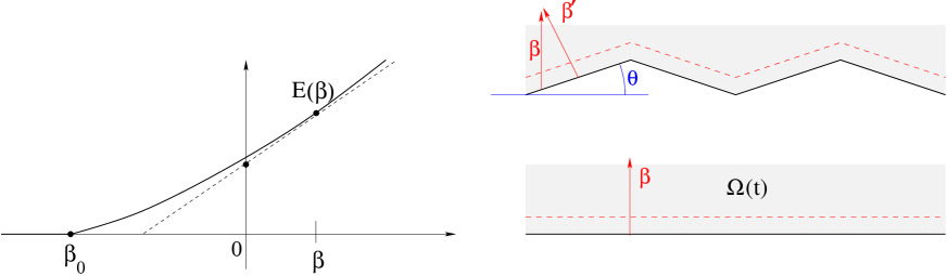
Figure 1: Left: an effort function $E$ that satisfies the assumption (1.6). Right: a geometric explanation of the necessity of this assumption.

Remark 1.4

The geometric meaning of the assumption (1.6) is shown in Fig. 1, left. Namely, the tangent line at $\beta$ has a positive intersection with the vertical axis. This assumption plays a crucial role for the lower semicontinuity of the cost functional in (1.4). Indeed, consider the situation in Figure 1, right. Here the contaminated region $\Omega(t)$ shrinks with inward normal speed $\beta>0$. We can slightly perturb its boundary, so that it oscillates with angle $\pm\theta$. In the first case the cost of the control, for a portion of the boundary parameterized by $s\in[s_{1},s_{2}]$, is computed by

$$\int_{s_{1}}^{s_{2}}E(\beta)\,ds,$$

where $ds$ denotes arclength along the boundary. In the perturbed case, the boundary length increases, while the normal speed decreases. This leads to

$$ds^{\prime}~{}=~{}{ds\over\cos\theta}\,,\qquad\qquad\beta^{\prime}~{}=~{}\beta\,\cos\theta.$$

The new total effort is

$$\int_{s_{1}}^{s_{2}}{E(\beta\cos\theta)\over\cos\theta}\,ds\,.$$

Differentiating w.r.t. $\theta$ we find

$${d\over d\theta}{E(\beta\cos\theta)\over\cos\theta}\Bigg{|}_{\theta=0}~{}=~{}0,\qquad\qquad{d^{2}\over d\theta^{2}}{E(\beta\cos\theta)\over\cos\theta}\Bigg{|}_{\theta=0}~{}=~{}E(\beta)-\beta\,E^{\prime}(\beta).$$

Therefore, if we want the wiggly profile to yield a larger or equal cost, the inequality (1.6) must be satisfied.

Example 1.1

Consider the basic case where

$$\left\{\begin{array}[]{rll}E(\beta)&=~{}\beta+1&\hbox{if}~{}~{}\beta\geq-1,\cr E(\beta)&=~{}0&\hbox{if}~{}~{}\beta\leq-1,\end{array}\right.\qquad\qquad\phi(s)~{}=~{}\left\{\begin{array}[]{cl}0&\hbox{if}\quad s\leq M,\cr+\infty&\hbox{if}\quad s>M.\end{array}\right.$$ (1.9)

In this case, with zero control effort, we obtain a set $\Omega(t)$ which expands in all directions with unit speed. On the other hand, the bound (1.3) on the instantaneous control effort allows us reduce the area of $\Omega(t)$ at rate $M$ per unit time. Calling

$$A(t)~{}=~{}m_{2}(\Omega(t)),\qquad P(t)~{}=~{}m_{1}(\partial\Omega(t))$$

respectively the area (i.e., the 2-dimensional Lebesgue measure) of $\Omega(t)$ and the perimeter of $\Omega(t)$, (i.e., the 1-dimensional Hausdorff measure of the boundary $\partial\Omega(t)$), we thus have

$${d\over dt}A(t)~{}=~{}P(t)-M.$$ (1.10)

The Null Controllability Problem (NCP) can thus be solved if we can reduce the perimeter $P(t)$ to a value smaller than $M$.

The remainder of the paper is organized as follows. Section 2 contains preliminary material. In particular, we reformulate the optimization problems in terms of sets with finite perimeter, and prove the one-sided Hölder estimate (2.16) on the area of the sets $\Omega(t)$, valid whenever the total cost of the control is bounded. In Section 3 we give a simple condition that ensures the solvability of the Null Controllability Problem. The existence of optimal solutions to (OP) is proved in Section 4, in the somewhat relaxed formulation (4.1). The following Sections 5 to 7 establish various necessary conditions for optimality. Finally, in Section 8 we discuss the geometric meaning of the necessary conditions, and give an example of a set-valued map $t\mapsto\Omega(t)$ that satisfies all these necessary conditions.

Based on these necessary conditions, we expect that at each time $t\in[0,T]$ the optimal control should concentrate all the effort along the portion of the boundary $\partial\Omega(t)$ with maximum curvature. At the present time, however, this remains on open question (see Conjecture 8.1), for two reasons:

• The existence of optimal solutions is here proved within a class of sets with finite perimeter, while our necessary conditions require piecewise ${\cal C}^{2}$ regularity.

• The set-valued functions $t\mapsto\Omega(t)$ which satisfy our optimality conditions may not be unique.

In earlier literature, several different models related to the control of a moving set have been analyzed in [6, 7, 9, 11, 13, 14]. Eradication problems for invasive biological species were studied in [3, 4].

2 Preliminaries

The instantaneous effort functional ${\cal E}(t)$ in (1.3) is naturally defined for moving sets with ${\cal C}^{1}$ boundary. Toward the analysis of optimization problems, it will be convenient to extend this definition to more general sets with finite perimeter [2, 16]. We shall thus work within the family of admissible sets

$${\cal A}~{}\doteq~{}\Big{\{}\Omega\subset\,]0,T[\,\times I\!\!R^{2}\,;~{}~{}\Omega~{}\hbox{is bounded and has bounded perimeter}\Big{\}}.$$ (2.1)

Calling ${\bf 1}_{\Omega}$ the characteristic function of $\Omega$, this implies that ${\bf 1}_{\Omega}\in BV$. In other words, the distributional gradient $\mu_{\Omega}\doteq D\,{\bf 1}_{\Omega}$ is a finite $I\!\!R^{3}$-valued Radon measure:

$$\int_{\Omega}\hbox{div}\,\varphi\,dx~{}=~{}-\int\varphi\cdot d\mu_{\Omega}\qquad\qquad\hbox{for all}~{}\varphi\in{\cal C}^{1}_{c}\bigl{(}]0,T[\,\times I\!\!R^{2}\,;~{}I\!\!R^{3}\bigr{)}.$$ (2.2)

Given a set $\Omega\in{\cal A}$, we consider the multifunction

$$t~{}\mapsto~{}\Omega(t)~{}\doteq~{}\bigl{\{}x\in I\!\!R^{2}\,;~{}(t,x)\in\Omega\bigr{\}}.$$ (2.3)

By possibly modifying ${\bf 1}_{\Omega}$ on a set of 3-dimensional measure zero, the map $t\mapsto{\bf 1}_{\Omega(t)}$ has bounded variation from $\,]0,T[\,$ into ${\bf L}^{1}(I\!\!R^{2})$. In particular, for every $0<t<T$, the one-sided limits

$${\bf 1}_{\Omega(t+)}~{}\doteq~{}\lim_{t\to t+}{\bf 1}_{\Omega(t)}\,,\qquad\qquad{\bf 1}_{\Omega(t-)}~{}\doteq~{}\lim_{t\to t-}{\bf 1}_{\Omega(t)}\,,$$ (2.4)

are well defined in ${\bf L}^{1}(I\!\!R^{2})$. This uniquely defines the sets $\Omega(t+)$, $\Omega(t-)$, up to a set of 2-dimensional Lebesgue measure zero. Throughout the following, we define the sets $\Omega(0)$ and $\Omega(T)$ in terms of

$${\bf 1}_{\Omega(0)}~{}\doteq~{}\lim_{t\to 0+}{\bf 1}_{\Omega(t)}\,,\qquad\qquad{\bf 1}_{\Omega(T)}~{}\doteq~{}\lim_{t\to T-}{\bf 1}_{\Omega(t)}\,.$$ (2.5)

We write ${\cal H}^{m}$ for the $m$-dimensional Hausdorff measure, while $\mu\,\llcorner V$ denotes the restriction of a measure $\mu$ to the set $V$. By $B(y,r)$ we denote the open ball centered at $y$ with radius $r$, while $S^{2}$ is the sphere of unit vectors in $I\!\!R^{3}$.

For every set of finite perimeter $\Omega\in{\cal A}$, its reduced boundary $\partial^{*}\Omega$ is defined to be the set of points $y=(t,x)\in\,]0,T[\,\times I\!\!R^{2}$ such that

$$\nu_{\Omega}(y)~{}\doteq~{}\lim_{r\downarrow 0}~{}{\mu_{\Omega}\bigl{(}B(y,r)\bigr{)}\over|\mu_{\Omega}|\bigl{(}B(y,r)\bigr{)}}$$ (2.6)

exists in $I\!\!R^{3}$ and satisfies $|\nu_{\Omega}(y)|=1$. The function $\nu_{\Omega}:\partial^{*}\Omega\mapsto S^{2}$ is called the generalized inner normal to $\Omega$. A fundamental theorem of De Giorgi [2, 16] implies that $\partial^{*}\Omega$ is countably 2-rectifiable and $|D{\bf 1}_{\Omega}|={\cal H}^{2}\llcorner\partial^{*}\Omega$.

In order to introduce a cost associated with each set $\Omega\in{\cal A}$, we observe that, in the smooth case, the (inward) normal velocity of the set $\Omega(t)$ at the point $(t,x)\in\partial^{*}\Omega$ is computed by

$$\beta~{}=~{}{-\nu_{0}\over\sqrt{\nu_{1}^{2}+\nu_{2}^{2}}}\,.$$ (2.7)

This leads us to consider the scalar measure

$$\mu~{}\doteq~{}\sqrt{\nu_{1}^{2}+\nu_{2}^{2}}\cdot E\left({-\nu_{0}\over\sqrt{\nu_{1}^{2}+\nu_{2}^{2}}}\right)\cdot{\cal H}^{2}\llcorner\partial^{*}\Omega\,,$$ (2.8)

and its projection $\widetilde{\mu}$ on the $t$-axis, defined by

$$\widetilde{\mu}(S)~{}=~{}\mu\Big{(}\bigl{\{}(t,x)\,;~{}t\in S,~{}x\in I\!\!R^{2}\bigr{\}}\Big{)}$$ (2.9)

for every Borel set $S\subset\,]0,T[\,$. We can now define a cost functional $\Psi(\Omega)$, for every $\Omega\in{\cal A}$, by setting

$$\Psi(\Omega)~{}\doteq~{}\left\{\begin{array}[]{cl}\displaystyle\int_{0}^{T}\phi\bigl{(}{\cal E}(t)\bigr{)}\,dt&\hbox{if}~{}~{}\widetilde{\mu}~{}\hbox{ is absolutely continuous with density ${\cal E}(t)$}\\ &\qquad\qquad\qquad\hbox{ w.r.t.~{}Lebesgue measure on $[0,T]$,}\\[11.38109pt] +\infty&\hbox{if}~{}~{}\widetilde{\mu}~{}\hbox{ is not absolutely continuous w.r.t.~{}Lebesgue measure.}\end{array}\right.$$ (2.10)

Remark 2.1

In the smooth case, (2.10) yields

$$\Psi(\Omega)~{}=~{}\int_{0}^{T}\phi\left(\int_{\partial\Omega(t)}E(\beta)\,d\sigma\right)dt.$$ (2.11)

where $d\sigma$ denotes the 1-dimensional measure along the boundary $\partial\Omega(t)$. Notice that, in the second alternative of (2.10), the infinite cost is motivated by the assumption of superlinear growth in (1.7).

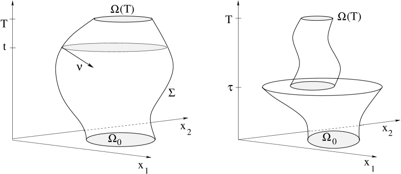
Figure 2: Left: the measure $\mu$ is absolutely continuous w.r.t. 2-dimensional Hausdorff measure on the surface $\Sigma\subset I\!\!R^{3}$ where $u$ has a jump. Right: an example where the projection of $\mu$ on the $t$-axis is not absolutely continuous w.r.t. 1-dimensional Lebesgue measure. Here $\widetilde{\mu}$ has a point mass at $t=\tau$.

Remark 2.2

If the assumptions (A1) hold, the function

$$L(\nu)~{}=~{}\sqrt{\nu_{1}^{2}+\nu_{2}^{2}}\cdot E\left({-\nu_{0}\over\sqrt{\nu_{1}^{2}+\nu_{2}^{2}}}\right)$$ (2.12)

is uniformly bounded on the set of all unit vectors $\nu=(\nu_{0},\nu_{1},\nu_{2})\in I\!\!R^{3}$. Hence the measure $\mu$, introduced at (2.8), is absolutely continuous w.r.t. 2-dimensional Hausdorff measure on the reduced boundary $\partial^{*}\Omega$. However, its projection $\widetilde{\mu}$ on the time axis may not be absolutely continuous w.r.t. 1-dimensional Lebesgue measure, as shown in Fig. 2, right.

We can now extend the function $L$ in (2.12) to a positively homogeneous function defined for all vectors ${\bf v}=(v_{0},v_{1},v_{2})\in I\!\!R^{3}$, by setting

$$L({\bf v})~{}\doteq~{}|{\bf v}|\,L\left({{\bf v}\over|{\bf v}|}\right)~{}=~{}\sqrt{v_{1}^{2}+v_{2}^{2}}\cdot E\left({-v_{0}\over\sqrt{v_{1}^{2}+v_{2}^{2}}}\right).$$ (2.13)

To analyze the lower semicontinuity of the corresponding integral functional, we check whether $L$ is convex. Restricted to the set where

$${-v_{0}\over\sqrt{v_{1}^{2}+v_{2}^{2}}}~{}>~{}\beta_{0}\,,$$

the partial derivatives are

$$L_{v_{0}}~{}=~{}\sqrt{v_{1}^{2}+v_{2}^{2}}\cdot E^{\prime}\left({-v_{0}\over\sqrt{v_{1}^{2}+v_{2}^{2}}}\right)\cdot{-1\over\sqrt{v_{1}^{2}+v_{2}^{2}}}~{}=~{}-E^{\prime}\left({-v_{0}\over\sqrt{v_{1}^{2}+v_{2}^{2}}}\right),$$

$$L_{v_{i}}~{}=~{}{v_{i}\over\sqrt{v_{1}^{2}+v_{2}^{2}}}\cdot E\left({-v_{0}\over\sqrt{v_{1}^{2}+v_{2}^{2}}}\right)+{v_{0}v_{i}\over v_{1}^{2}+v_{2}^{2}}E^{\prime}\left({-v_{0}\over\sqrt{v_{1}^{2}+v_{2}^{2}}}\right),\qquad\qquad i=1,2,$$

$$L_{v_{0}v_{0}}~{}=~{}E^{\prime\prime}\left({-v_{0}\over\sqrt{v_{1}^{2}+v_{2}^{2}}}\right)\cdot{1\over\sqrt{v_{1}^{2}+v_{2}^{2}}}~{}\geq~{}0\,,$$

$$L_{v_{0}v_{i}}~{}=~{}E^{\prime\prime}\left({-v_{0}\over\sqrt{v_{1}^{2}+v_{2}^{2}}}\right)\cdot(-v_{0}v_{i})\cdot(v_{1}^{2}+v_{2}^{2})^{-3/2}\,,$$

$$\begin{array}[]{rl}L_{v_{i}v_{i}}&=\displaystyle{1\over\sqrt{v_{1}^{2}+v_{2}^{2}}}\Big{(}1-{v_{i}^{2}\over v_{1}^{2}+v_{2}^{2}}\Big{)}\,E\left({-v_{0}\over\sqrt{v_{1}^{2}+v_{2}^{2}}}\right)+{v_{0}(v_{1}^{2}+v_{2}^{2})-v_{0}v_{i}^{2}\over(v_{1}^{2}+v_{2}^{2})^{2}}E^{\prime}\left({-v_{0}\over\sqrt{v_{1}^{2}+v_{2}^{2}}}\right)\\[8.53581pt] &\qquad\displaystyle+{v_{0}^{2}v_{i}^{2}\over(v_{1}^{2}+v_{2}^{2})^{5/2}}E^{\prime\prime}\left({-v_{0}\over\sqrt{v_{1}^{2}+v_{2}^{2}}}\right),\end{array}$$

$$\begin{array}[]{lr}\displaystyle L_{v_{i}v_{j}}=-{v_{i}v_{j}\over(v_{1}^{2}+v_{2}^{2})^{3/2}}E\left({-v_{0}\over\sqrt{v_{1}^{2}+v_{2}^{2}}}\right)-{v_{0}v_{i}v_{j}\over(v_{1}^{2}+v_{2}^{2})^{2}}E^{\prime}\left({-v_{0}\over\sqrt{v_{1}^{2}+v_{2}^{2}}}\right)\\[8.53581pt] \qquad\qquad\displaystyle+~{}{v_{0}^{2}v_{i}v_{j}\over(v_{1}^{2}+v_{2}^{2})^{5/2}}E^{\prime\prime}\left({-v_{0}\over\sqrt{v_{1}^{2}+v_{2}^{2}}}\right),\qquad\qquad i=1,2\quad i\neq j\end{array}$$

Since $L$ is positively homogeneous, and invariant under rotations in the $v_{1},v_{2}$ coordinates, it suffices to compute the Hessian matrix of partial derivatives in the special case where ${\bf v}=(v_{0},v_{1},v_{2})=(v_{0},1,0)$. At this particular point, the above computations yield

$$D^{2}L({\bf v})~{}=~{}\begin{pmatrix}E^{\prime\prime}(-v_{0})&-v_{0}E^{\prime\prime}(-v_{0})&0\\ -v_{0}E^{\prime\prime}(-v_{0})&v_{0}^{2}E^{\prime\prime}(-v_{0})&0\\ 0&0&v_{0}E^{\prime}(-v_{0})+E(-v_{0})\end{pmatrix}.$$ (2.14)

The eigenvalues of this matrix are found to be

$$0\,,\qquad(1+v_{0}^{2})\,E^{\prime\prime}(-v_{0})\,,\qquad v_{0}E^{\prime}(-v_{0})+E(-v_{0}).$$

All of these are non-negative, provided that the effort function satisfies (1.6). We notice that the vector ${\bf v}=(v_{0},1,0)$ is itself an eigenvector of the Hessian matrix $D^{2}L({\bf v})$ at (2.14), with zero as corresponding eigenvalue. This is consistent with the fact that, by (2.13), $L$ is linear homogeneous along each ray through the origin.

The above computations show that the Hessian matrix of $L$ is non-negative definite at every point outside the cone

$$\Gamma~{}=~{}\Big{\{}(v_{0},v_{1},v_{2})\,;~{}v_{0}\geq-\beta_{0}\sqrt{v_{1}^{2}+v_{2}^{2}}\,\Big{\}}.$$ (2.15)

By (1.5), $L$ vanishes on the convex cone $\Gamma$. We thus conclude that $L$ is convex on the entire space $I\!\!R^{3}$. In view of (1.5), the cost function $L$ in (2.12) does not pose any restriction on how fast the set $\Omega(t)$ expands, but it penalizes the rate at which $\Omega(t)$ shrinks. This leads to the following one-sided Hölder estimate:

Lemma 2.1

Let the assumptions (A1)-(A2) hold, and let $\Omega\in{\cal A}$ be such that $\Psi(\Omega)<+\infty$. Then there exists a constant $C$ such that

$$m_{2}\bigl{(}\Omega(\tau+)\setminus\Omega(\tau^{\prime}-)\bigr{)}~{}\leq~{}C(\tau^{\prime}-\tau)^{p-1\over p}\qquad\hbox{for all}~{}0<\tau<\tau^{\prime}<T.$$ (2.16)

Proof. 1. Given $\tau<\tau^{\prime}$, consider the set

$$\Sigma^{-}~{}\doteq~{}\Big{\{}(t,x)\in\partial^{*}\Sigma\,;~{}\tau<t<\tau^{\prime},~{}\nu_{0}<0\Big{\}}.$$ (2.17)

Observing that $E(\beta)$ is uniformly positive for $\beta\geq 0$, define the constant

$$c_{0}~{}\doteq~{}\min_{|\nu|=1,\,\nu_{0}\geq 0}~{}L(\nu)~{}=~{}\min_{|\nu|=1,\,\nu_{0}\geq 0}\bigg{\{}\sqrt{\nu_{1}^{2}+\nu_{2}^{2}}\cdot E\left({-\nu_{0}\over\sqrt{\nu_{1}^{2}+\nu_{2}^{2}}}\right)\bigg{\}}.$$

One now has the estimate

$$m_{2}\bigl{(}\Omega(\tau+)\setminus\Omega(\tau^{\prime}-)\bigr{)}~{}\leq~{}{\cal H}^{2}(\Sigma^{-})~{}~{}\leq~{}{1\over c_{0}}\int_{\Sigma^{-}}L(\nu)\,d{\cal H}^{2}\,.$$ (2.18)

2. In view of the assumption (1.7), using Hölder’s inequality with ${1\over p}+{1\over q}=1$, we obtain

$$\begin{array}[]{l}\displaystyle\int_{\tau}^{\tau^{\prime}}1\cdot{\cal E}(t)\,dt~{}\leq~{}(\tau^{\prime}-\tau)^{1/q}\cdot\left(\int_{\tau}^{\tau^{\prime}}\bigl{[}{\cal E}(t)\bigr{]}^{p}\,dt\right)^{1/p}\\[11.38109pt] \displaystyle\qquad\leq~{}(\tau^{\prime}-\tau)^{1/q}\cdot\left(\int_{\tau}^{\tau^{\prime}}\left[{1\over C_{1}}\phi\bigl{(}{\cal E}(t)\bigr{)}+C_{2}\right]\,dt\right)^{1/p}~{}\leq~{}C_{3}\,(\tau^{\prime}-\tau)^{1/q},\end{array}$$

for a suitable constant $C_{3}$. Together with (2.18), this yields

$$m_{2}\bigl{(}\Omega(\tau+)\setminus\Omega(\tau^{\prime}-)\bigr{)}~{}\leq~{}{1\over c_{0}}\int_{\tau}^{\tau^{\prime}}{\cal E}(t)\,dt~{}\leq~{}{C_{3}\over c_{0}}\,(\tau^{\prime}-\tau)^{1/q},$$

completing the proof. MM     

Remark 2.3

If $\phi(s)=+\infty$ for $s>M$, then (2.16) can be replaced by the one-sided Lipschitz estimate:

$$m_{2}\bigl{(}\Omega(\tau+)\setminus\Omega(\tau^{\prime}-)\bigr{)}~{}\leq~{}C(\tau^{\prime}-\tau)\qquad\hbox{for all}~{}0<\tau<\tau^{\prime}<T.$$ (2.19)

3 Existence of eradication strategies

The next result provides a simple condition for the solvability of the Null Controllability Problem (NCP). Thinking of $\Omega(t)$ as the region contaminated by an invasive biological species, this yields a strategy that eradicates the contamination in finite time.

Theorem 3.1

Let the assumptions (A1) hold. Let $\Omega_{0}$ be a compact set whose convex closure $\widehat{\Omega}_{0}=co\,\Omega_{0}$ has perimeter which satisfies

$$E(0)\cdot m_{1}(\partial\widehat{\Omega}_{0})~{}<~{}M.$$ (3.1)

Then the null controllability problem (NCP) has a solution.

Proof. 1. By (3.1) and the continuity of $E$, there exists a speed $\beta_{1}>0$ small enough so that

$$E(\beta_{1})\cdot m_{1}\bigl{(}\partial\widehat{\Omega}_{0}\bigr{)}~{}\leq~{}M.$$ (3.2)

We now define the convex subsets

$$\widehat{\Omega}(t)~{}=~{}\Big{\{}x\in I\!\!R^{2}\,;~{}~{}B(x,\,\beta_{1}t)\subseteq\widehat{\Omega}_{0}\Big{\}}.$$ (3.3)

Notice that these sets are obtained starting from $\widehat{\Omega}_{0}$, and letting every boundary point $x\in\partial\widehat{\Omega}(t)$ move with inward normal speed $\beta_{1}$. Since the boundaries of these sets have decreasing length, the total effort required by this strategy at time $t\geq 0$ is

$$\widehat{\cal E}(t)~{}=~{}E(\beta_{1})\cdot m_{1}\bigl{(}\partial\widehat{\Omega}(t)\bigr{)}~{}\leq~{}E(\beta_{1})\cdot m_{1}\bigl{(}\partial\widehat{\Omega}_{0}\bigr{)}~{}\leq~{}M.$$

The set $\widehat{\Omega}(t)$ shrinks to the empty set within a finite time $T$, which can be estimated in terms of the diameter of $\Omega_{0}$. Namely,

$$T~{}<~{}{\hbox{diam}(\widehat{\Omega}_{0})\over\beta_{1}}~{}=~{}{\hbox{diam}(\Omega_{0})\over\beta_{1}}\,.$$

2. Next, consider the smaller sets

$$\Omega(t)~{}\doteq~{}\widehat{\Omega}(t)\cap B\bigl{(}\Omega_{0}\,,~{}|\beta_{0}|t\bigr{)}.$$

By construction, at each time $t\in[0,T]$ the boundary $\partial\Omega(t)$ either touches the boundary $\partial\widehat{\Omega}(t)$, ore else it expands with normal speed $|\beta_{0}|$. This implies

$${\cal E}(t)~{}=~{}\int_{\partial\Omega(t)}E\bigl{(}\beta(t,x)\bigr{)}\,d\sigma~{}=~{}\int_{\partial\Omega(t)\cap\partial\widehat{\Omega}(t)}E(\beta_{1})\,d\sigma~{}\leq~{}\widehat{\cal E}(t)~{}\leq~{}M.$$

Therefore, the multifunction $t\mapsto\Omega(t)$ satisfies (1.3). 3. It remains to prove that the initial condition is satisfied, in the sense that

$$\lim_{t\to 0+}\,\bigl{\|}{\bf 1}_{\Omega(t)}-{\bf 1}_{\Omega_{0}}\bigr{\|}_{{\bf L}^{1}(I\!\!R^{2})}~{}=~{}0.$$ (3.4)

Toward this goal, we observe that, since $\Omega_{0}$ is compact,

$$\lim_{t\to 0+}m_{2}\Big{(}B\bigl{(}\Omega_{0},\,2|\beta_{0}|t\bigr{)}\Big{)}~{}=~{}m_{2}(\Omega_{0}).$$ (3.5)

Hence

$$\lim_{t\to 0+}m_{2}\bigl{(}\Omega(t)\setminus\Omega_{0}\bigl{)}~{}=~{}0.$$ (3.6)

On the other hand, observing that

$$\Omega_{0}\setminus\Omega(t)~{}\subseteq~{}\bigl{\{}x\in\widehat{\Omega}_{0}\,;~{}~{}d(x,\partial\widehat{\Omega}_{0})~{}\leq~{}|\beta_{1}|t\Bigr{\}},$$

we obtain

$$\lim_{t\to 0+}m_{2}\bigl{(}\Omega_{0}\setminus\Omega(t)\bigr{)}~{}\leq~{}\lim_{t\to 0+}|\beta_{1}|\,t\cdot m_{1}(\partial\widehat{\Omega})~{}=~{}0.$$ (3.7)

Together, (3.6) and (3.7) yield (3.4). MM     

4 Existence of optimal strategies

To achieve the existence of an optimal strategy $t\mapsto\Omega(t)$, we need to somewhat relax the formulation of the problem (OP). We recall that a subset $\Omega\subset\,]0,T[\,\times I\!\!R^{2}$ determines the multifunction $t\mapsto\Omega(t)$ as in (2.3). Moreover, assuming that $\Omega\in{\cal A}$ is bounded and has finite perimeter, the initial and terminal values $\Omega(0)$ and $\Omega(T)$ are uniquely determined by (2.5). Recalling the functional $\Psi(\Omega)$ introduced at (2.10), and denoting by $m_{2}$, $m_{3}$ respectively the 2- and 3-dimensional Lebesgue measure, we thus consider the problem of Optimal Set Motion:

• Given a bounded initial set $\Omega_{0}\subset I\!\!R^{2}$, find a set $\Omega\subset\,]0,T[\,\times I\!\!R^{2}$ which minimizes the functional

  $${\cal J}(\Omega)~{}\doteq~{}\Psi(\Omega)+c_{1}m_{3}(\Omega)+c_{2}\,m_{2}\bigl{(}\Omega(T)\bigr{)}\,,$$ (4.1)

  among all sets $\Omega\in{\cal A}$ such that $\Omega(0)=\Omega_{0}$.

Aim of this section is to prove the existence of solutions to the above optimization problem.

Theorem 4.1

Let $E,\phi$ satisfy the assumptions (A1)-(A2). Then, for any compact set $\Omega_{0}\subset I\!\!R^{2}$ with finite perimeter and any $T,c_{1},c_{2}>0$, the problem (OSM) has an optimal solution.

Proof. 1. We start with the trivial observation that ${\cal J}(\Omega)\geq 0$ for every $\Omega\in{\cal A}$. Moreover, choosing $\Omega=\,]0,T[\,\times\Omega_{0}$, so that $\Omega(t)\equiv{\Omega_{0}}$ for all $t\in[0,1]$, we obtain an admissible set $\Omega\in{\cal A}$ with ${\cal J}(\Omega)<+\infty$. We can thus consider a minimizing sequence of sets $\Omega_{n}\in{\cal A}$ such that, as $n\to\infty$,

$${\cal J}(\Omega_{n})~{}\to~{}{\cal J}_{min}~{}\doteq~{}\inf_{\Omega\in{\cal A}}{\cal J}(\Omega)\,.$$

Without loss of generality we can assume that the sets

$$\Omega_{n}(t)~{}\doteq~{}\bigl{\{}x\in I\!\!R^{2}\,;~{}(t,x)\in\Omega_{n}\bigr{\}}$$

are contained in the neighborhood of radius $|\beta_{0}|t$ around $\Omega_{0}$:

$$\Omega_{n}(t)~{}\subseteq~{}B\bigl{(}\Omega_{0}\,;~{}|\beta_{0}|t\bigr{)}$$ (4.2)

for every $n\geq 1$ and $t\geq 0$. Otherwise, we can simply replace each set $\Omega_{n}(t)$ with the intersection $\Omega_{n}(t)\cap B\bigl{(}\Omega_{0}\,;~{}|\beta_{0}|t\bigr{)}$, without increasing the total cost. 2. In the next two steps we prove a uniform bound on perimeters of the sets $\Omega_{n}\subset I\!\!R^{3}$.

Choose a speed $\beta^{*}<0$ and constants $\delta,\lambda>0$ such that (see Fig. 3, left)

$$E(\beta^{*})~{}=~{}\delta~{}>~{}0,\qquad E(\beta)~{}\geq~{}\delta+\lambda\,(\beta-\beta^{*})\qquad\hbox{for all}~{}\beta\geq\beta^{*}\,.$$ (4.3)

We split the reduced boundary in the form

$$\partial^{*}\Omega_{n}~{}=~{}\Sigma_{n}^{-}\cup\Sigma_{n}^{+}\,,$$ (4.4)

so that the following holds. Calling $\nu=(\nu_{0},\nu_{1},\nu_{2})$ the normal vector at the point $(t,x)\in\partial^{*}\Omega$, and defining the inner normal velocity $\beta_{n}=\beta_{n}(t,x)$ as in (2.7), one has

$$\left\{\begin{array}[]{rl}\beta_{n}(t,x)~{}\leq~{}\beta^{*}&\hbox{if}\quad(t,x)\in\Sigma_{n}^{-}\,,\\[5.69054pt] \beta_{n}(t,x)~{}>~{}\beta^{*}&\hbox{if}\quad(t,x)\in\Sigma_{n}^{+}\,.\end{array}\right.$$ (4.5)

By (A2) we can find a constant $b_{0}>0$ such that

$$\phi(s)~{}\geq~{}s-b_{0}\qquad\qquad\hbox{for all}~{}s\in I\!\!R_{+}\,.$$ (4.6)

In view of (1.5), this implies

$$\begin{array}[]{rl}\displaystyle\int_{0}^{T}\phi\bigl{(}{\cal E}_{n}(t)\bigr{)}\,dt&\displaystyle\geq~{}\int_{\Sigma_{n}}\sqrt{\nu_{1}^{2}+\nu_{2}^{2}}\cdot E\left({-\nu_{0}\over\sqrt{\nu_{1}^{2}+\nu_{2}^{2}}}\right)\,d{\cal H}^{2}-b_{0}T.\end{array}$$ (4.7)

On the domain $\Sigma_{n}^{+}$, where

$$\beta~{}\doteq~{}{-\nu_{0}\over\sqrt{\nu_{1}^{2}+\nu_{2}^{2}}}~{}\geq~{}\beta^{*},$$ (4.8)

by (4.3) we have

$$\sqrt{\nu_{1}^{2}+\nu_{2}^{2}}\cdot E\left({-\nu_{0}\over\sqrt{\nu_{1}^{2}+\nu_{2}^{2}}}\right)~{}\geq~{}\sqrt{\nu_{1}^{2}+\nu_{2}^{2}}\left(\delta+\lambda\Big{(}{-\nu_{0}\over\sqrt{\nu_{1}^{2}+\nu_{2}^{2}}}-\beta^{*}\Big{)}\right)~{}\geq~{}c_{3}$$ (4.9)

for some constant $c_{3}>0$. Together with (4.7), this yields

$$\int_{\Sigma_{n}^{+}}d{\cal H}^{2}~{}\leq~{}{1\over c_{3}}\left[\int_{0}^{T}\phi\bigl{(}{\cal E}_{n}(t)\bigr{)}\,dt+b_{0}T\right].$$ (4.10)

Figure 3: Left: a lower bound on the function $E(\beta)$, considered at (4.3). Right: since the cost function $\phi$ has superlinear growth, it admits a lower bound of the form (4.6).

3. On the domain $\Sigma_{n}^{-}$ where (4.8) fails, we have a lower bound

$$\nu_{0}~{}\geq~{}c_{4}~{}>~{}0,$$ (4.11)

for some positive constant $c_{4}$. We can now write

$$\begin{array}[]{l}\displaystyle m_{2}\Big{(}B\bigl{(}\Omega_{0},\,|\beta_{0}|T\bigr{)}\Big{)}~{}\geq~{}m_{2}\bigl{(}\Omega_{n}(T)\bigr{)}-m_{2}\bigl{(}\Omega_{n}(0)\bigr{)}\\[11.38109pt] \qquad\displaystyle=~{}\int_{\Sigma_{n}^{+}\cup\Sigma_{n}^{-}}\nu_{0}\,d{\cal H}^{2}~{}\geq~{}c_{4}\int_{\Sigma_{n}^{-}}d{\cal H}^{2}-\int_{\Sigma_{n}^{+}}d{\cal H}^{2}.\end{array}$$ (4.12)

Combining (4.12) with (4.10) one obtains

$$\int_{\Sigma_{n}^{-}}d\Sigma~{}\leq~{}{1\over c_{4}}\left\{m_{2}\Big{(}B\bigl{(}\Omega_{0},\,|\beta_{0}|T\bigr{)}\Big{)}+{1\over c_{3}}\left[\int_{0}^{T}\phi\bigl{(}{\cal E}_{n}(t)\bigr{)}\,dt+b_{0}T\right]\right\}.$$ (4.13)

We notice that, for a minimizing sequence, the integrals $\int{\cal E}_{n}(t)dt$ must be bounded, because they are part of the cost functional (2.10).

Together, the two inequalities (4.10) and (4.13) thus yield a uniform bound on the 2-dimensional measure ${\cal H}^{2}(\Sigma_{n})$, i.e. on the total variation of the function $u_{n}$, for every $n\geq 1$.

4. Thanks to the uniform BV bound, by possibly taking a subsequence, a compactness argument (see Theorem 12.26 in [16]) yields the the existence of a bounded set with finite perimeter $\Omega\in{\cal A}$ such that the following holds. As $n\to\infty$, one has the convergence

$$\Big{\|}{\bf 1}_{\Omega_{n}}-{\bf 1}_{\Omega}\Big{\|}_{{\bf L}^{1}\bigl{(}]0,T[\,\times I\!\!R^{2}\bigr{)}}~{}\to~{}0,$$ (4.14)

together with the weak convergence of measures

$$\mu_{\Omega_{n}}~{}\rightharpoonup~{}\mu_{\Omega}\,.$$ (4.15)

Next, the assumption of superlinear growth (1.7) implies

$$\int_{0}^{T}\phi\bigl{(}{\cal E}_{n}(t)\bigr{)}dt~{}\geq~{}C_{1}\int_{0}^{T}\bigl{[}{\cal E}_{n}(t)\bigr{]}^{p}\,dt-C_{2}T.$$ (4.16)

Therefore, the functions ${\cal E}_{n}$ are uniformly bounded in ${\bf L}^{p}$. Since $p>1$, we can extract a weakly convergent subsequence ${\cal E}_{n}\rightharpoonup{\cal E}_{\infty}\in{\bf L}^{p}([0,T],I\!\!R)$. We observe that ${\cal E}_{\infty}$ yields the density of the measure $\widetilde{\mu}_{\infty}$, defined as the weak limit of the projected measures $\widetilde{\mu}_{n}$. 5. To prove a lower semicontinuity result, we first replace $\phi$ with a globally Lipschitz, convex function

$$\phi_{m}(s)~{}=~{}\sup_{0\leq a\leq m,\,b\in I\!\!R}\Big{\{}as+b\,;~{}~{}at+b\leq\phi(t)\quad\hbox{for all}~{}t\in I\!\!R\Big{\}}.$$ (4.17)

Notice that the function $\phi_{m}$ is Lipschitz continuous with constant $m$. Its graph is the upper envelope of all straight lines with slope $\leq m$ that lie below the graph of $\phi$.

Let $\varepsilon>0$ be given. Choosing $m$ large enough, we achieve

$$\int_{0}^{T}\phi\bigl{(}{\cal E}_{\infty}(t)\bigr{)}\,dt~{}\leq~{}\varepsilon+\int_{0}^{T}\phi_{m}\bigl{(}{\cal E}_{\infty}(t)\bigr{)}\,dt.$$ (4.18)

6. Next, we partition the interval $[0,T]$ into finitely many subintervals $I_{j}=[t_{j-1},t_{j}]$, $j=1,\ldots,N$, so that the difference between ${\cal E}_{\infty}$ and its average value over each subinterval is bounded by

$$\sum_{1\leq j\leq N}\int_{t_{j-1}}^{t_{j}}\left|{\cal E}_{\infty}(t)--\!\!\!\!\!\!\int_{t_{j-1}}^{t_{j}}{\cal E}_{\infty}(\tau)d\tau\right|dt~{}<~{}{\varepsilon\over m}\,.$$ (4.19)

The Lipschitz continuity of the function $\phi_{m}$ now yields

$$\sum_{1\leq j\leq N}\int_{t_{j-1}}^{t_{j}}\left|\phi_{m}\bigl{(}{\cal E}_{\infty}(t)\bigr{)}-\phi_{m}\left(-\!\!\!\!\!\!\int_{t_{j-1}}^{t_{j}}{\cal E}_{\infty}(\tau)d\tau\right)\right|dt~{}<~{}\varepsilon\,,$$ (4.20)

$$\int_{0}^{T}\phi_{m}\bigl{(}{\cal E}_{\infty}(t)\bigr{)}\,dt~{}\leq~{}\varepsilon+\sum_{1\leq j\leq N}(t_{j}-t_{j-1})\phi_{m}\left(-\!\!\!\!\!\!\int_{t_{j-1}}^{t_{j}}{\cal E}_{\infty}(\tau)d\tau\right).$$ (4.21)

7. We now study the relation between ${\cal E}_{\infty}(t)$ and the instantaneous effort ${\cal E}(t)$ associated to the limit set $\Omega$.

Since the function $L$ in (2.12) is convex, for any $0<\tau<\tau^{\prime}<T$ we can use a lower semicontinuity result for anisotropic functionals (see Theorem 20.1 in [16]) and conclude

$$\begin{array}[]{rl}\displaystyle\int_{\tau}^{\tau^{\prime}}{\cal E}(t)\,dt&\displaystyle=~{}\int_{\partial^{*}\Omega\cap\{\tau<t<\tau^{\prime}\}}L(\nu)\,d{\cal H}^{2}~{}\leq~{}\liminf_{n\to\infty}\int_{\partial^{*}\Omega\cap\{\tau<t<\tau^{\prime}\}}L(\nu_{n})\,d{\cal H}^{2}\\[11.38109pt] &\displaystyle=~{}\liminf_{n\to\infty}\int_{\tau}^{\tau^{\prime}}{\cal E}_{n}(t)\,dt~{}=~{}\int_{\tau}^{\tau^{\prime}}{\cal E}_{\infty}(t)\,dt\,.\end{array}$$ (4.22)

Since $\tau,\tau^{\prime}$ were arbitrary, this implies ${\cal E}(t)\leq{\cal E}_{\infty}(t)$ for a.e. $t\in[0,T]$. Next, by Jensen’s inequality and the convexity of $\phi_{m}$ it follows

$$(t_{j}-t_{j-1})\phi_{m}\left(-\!\!\!\!\!\!\int_{t_{j-1}}^{t_{j}}{\cal E}_{n}(\tau)d\tau\right)~{}\leq~{}\int_{t_{j-1}}^{t_{j}}\phi_{m}\bigl{(}{\cal E}_{n}(t)\bigr{)}dt\,.$$ (4.23)

Summing over $j=1,\ldots,N$, and using (4.21) and (4.18), (4.20), we conclude

$$\begin{array}[]{l}\displaystyle\int_{0}^{T}\phi\bigl{(}{\cal E}(t)\bigr{)}\,dt~{}\leq~{}\int_{0}^{T}\phi\bigl{(}{\cal E}_{\infty}(t)\bigr{)}\,dt~{}\leq~{}\varepsilon+\int_{0}^{T}\phi_{m}\bigl{(}{\cal E}_{\infty}(t)\bigr{)}\,dt\\[11.38109pt] \displaystyle\qquad\leq 2\varepsilon+\sum_{1\leq j\leq N}(t_{j}-t_{j-1})\phi_{m}\left(-\!\!\!\!\!\!\int_{t_{j-1}}^{t_{j}}{\cal E}_{\infty}(\tau)d\tau\right)\\[11.38109pt] \displaystyle\qquad=2\varepsilon+\sum_{1\leq j\leq N}(t_{j}-t_{j-1})\phi_{m}\left(\lim_{n\to\infty}-\!\!\!\!\!\!\int_{t_{j-1}}^{t_{j}}{\cal E}_{n}(\tau)d\tau\right)\\[11.38109pt] \qquad\displaystyle=~{}2\varepsilon+\lim_{n\to\infty}\sum_{1\leq j\leq N}(t_{j}-t_{j-1})\phi_{m}\left(-\!\!\!\!\!\!\int_{t_{j-1}}^{t_{j}}{\cal E}_{n}(\tau)d\tau\right)\\[11.38109pt] \qquad\displaystyle\leq~{}2\varepsilon+\liminf_{n\to\infty}\int_{0}^{T}\phi_{m}\bigl{(}{\cal E}_{n}(t)\bigr{)}\,dt~{}\leq~{}2\varepsilon+\liminf_{n\to\infty}\int_{0}^{T}\phi\bigl{(}{\cal E}_{n}(t)\bigr{)}\,dt\,.\end{array}$$ (4.24)

8. As $n\to\infty$, the convergence (4.14) immediately implies

$$m_{3}(\Omega_{n})~{}\to~{}m_{3}(\Omega).$$ (4.25)

Moreover, since the map $t\mapsto{\bf 1}_{\Omega(t)}\in{\bf L}^{1}(I\!\!R^{2})$ has bounded variation, given $\varepsilon>0$ we can find $\delta>0$ such that

$$\left|m_{2}(\Omega(T)\big{)}-{1\over\delta}\int_{T-\delta}^{T}m_{2}(\Omega(t)\big{)}\,dt\right|~{}<~{}\varepsilon.$$ (4.26)

On the other hand, by the one-sided estimate in Lemma 2.1 it follows

$$m_{2}\bigl{(}\Omega_{n}(\tau)\setminus\Omega_{n}(T)\bigr{)}~{}\leq~{}C\,(T-\tau)^{p-1\over p},$$

for some constant $C$ independent of $T,\tau$, and $n$. Therefore, we can find $\delta>0$ such that

$$m_{2}\bigl{(}\Omega_{n}(T)\bigr{)}~{}\geq~{}{1\over\delta}\int_{T-\delta}^{T}m_{2}\bigl{(}\Omega_{n}(t)\bigr{)}\,dt-\varepsilon$$

for every $n\geq 1$. Since

$${1\over\delta}\int_{T-\delta}^{T}m_{2}\bigl{(}\Omega_{n}(t)\bigr{)}\,dt~{}\to~{}{1\over\delta}\int_{T-\delta}^{T}m_{2}\bigl{(}\Omega(t)\bigr{)}\,dt\,,$$

we conclude

$$m_{2}\bigl{(}\Omega(T)\bigr{)}~{}\leq~{}\liminf_{n\to\infty}m_{2}\bigl{(}\Omega_{n}(T)\bigr{)}+2\varepsilon.$$ (4.27)

9. Combining (4.24), (4.25), and (4.27), since $\varepsilon>0$ was arbitrary we conclude

$${\cal J}(\Omega)~{}\doteq~{}\int_{0}^{T}{\cal E}(t)\,dt+c_{1}\,m_{3}(\Omega)+c_{2}\,m_{2}\bigl{(}\Omega(T)\bigr{)}~{}\leq~{}\liminf_{n\to\infty}{\cal J}(\Omega_{n}).$$ (4.28)

10. It remains to prove that the limit set $\Omega$ satisfies the initial condition (3.4). Since $\Omega_{0}$ is compact, by (4.2) we immediately have

$$\lim_{t\to 0+}m_{2}\bigl{(}\Omega(t)\setminus\Omega_{0}\bigr{)}~{}\leq~{}\lim_{t\to 0+}m_{2}\Big{(}B\bigl{(}\Omega_{0};\,|\beta_{0}|t\bigr{)}\setminus\Omega_{0}\Big{)}~{}=~{}0.$$ (4.29)

On the other hand, by (2.16) for every $t>0$ one has

$$m_{2}\bigl{(}\Omega_{0}\setminus\Omega_{n}(t)\bigr{)}~{}\leq~{}C\,t^{p-1\over p},$$

for a suitable constant $C$ independent of $t$ and $n$. Taking the limit as $n\to\infty$ one obtains

$$m_{2}\bigl{(}\Omega_{0}\setminus\Omega(t)\bigr{)}~{}\leq~{}C\,t^{p-1\over p}.$$ (4.30)

Together, (4.29) and (4.30) yield the convergence ${\bf 1}_{\Omega(t)}\to{\bf 1}_{\Omega_{0}}$ in ${\bf L}^{1}(I\!\!R^{2})$, completing the proof. MM     

By entirely similar arguments one can prove the existence of an optimal solution for the minimum time problem.

Theorem 4.2

Let the functions $E$ satisfy the assumptions (A1) and let $M>0$ be given. Let $\Omega_{0}\subset I\!\!R^{2}$ be a compact set with finite perimeter such that the null controllability problem (NCP) has a solution. Then the minimum time problem (MTP) has an optimal solution.

Proof. Consider a minimizing sequence $(\Omega_{n})_{n\geq 1}$. Calling $\Omega_{n}(t)=\bigl{\{}x\,;~{}(t,x)\in\Omega_{n}\bigl{\}}$, we thus have

$$m_{2}\bigl{(}\Omega_{n}(T_{n})\bigr{)}~{}=~{}0,$$ (4.31)

with $T_{n}\downarrow T$. The same arguments used in the proof of Theorem 4.1 yield a uniform bound on the perimeter of $\Omega_{n}$. By possibly taking a subsequence we obtain the strong convergence ${\bf 1}_{\Omega_{n}}\to{\bf 1}_{\Omega}$. By assumption, ${\cal E}_{n}(t)\leq M$ for every $t,n$. Calling ${\cal E}(t)$ the effort corresponding to $\Omega$, and ${\cal E}_{\infty}$ the weak limit of the functions ${\cal E}_{n}$, the previous arguments yield ${\cal E}(t)\leq{\cal E}_{\infty}(t)\leq M$ for all $t\geq 0$.

In the present setting, for any $n\geq 1$, we have the one-sided Lipschitz estimate (2.19). In particular, taking $\tau=T_{n}$ and $\tau^{\prime}=T$, we obtain

$$m_{2}\big{(}\Omega_{n}(T)\bigr{)}~{}\leq~{}C_{4}(T_{n}-T).$$

Taking the limit as $n\to\infty$, this implies $m_{2}\bigl{(}\Omega(T)\bigr{)}=0$. Hence the set-valued function $t\mapsto\Omega(t)$ provides an optimal solution to the minimum time problem. MM     

5 Necessary conditions for optimality

Let $t\mapsto\Omega(t)\subset I\!\!R^{2}$ be an optimal solution for the problem (OP) of control of a moving set. Aim of this section is to derive a set of necessary conditions for optimality, in the form of a Pontryagin maximum principle [10, 12, 15]. For this purpose, somewhat stronger regularity assumptions will be needed. As shown in Fig. 4, we consider the unit circumference $S=\{\xi\in I\!\!R^{2}\,;~{}|\xi|=1\}$ and, for each $t\in[0,T]$, we assume that

$$\xi~{}\mapsto~{}x(t,\xi)~{}\in~{}\partial\Omega(t)$$

is a ${\cal C}^{2}$ parameterization of the boundary of $\Omega(t)$ (oriented counterclockwise), satisfying

• There exists a constant $C>0$ such that

  $${1\over C}~{}\leq~{}\bigl{|}x_{\xi}(t,\xi)\bigr{|}~{}\leq~{}C\qquad\hbox{for all}~{}(t,\xi)\in[0,T]\times S,$$ (5.1)

  Moreover, for every $\xi\in S$ the trajectory $t\mapsto x(t,\xi)$ is orthogonal to the boundary $\partial\Omega(t)$ at every time $t$. Namely,

  $$x_{t}(t,\xi)~{}=~{}\beta(t,\xi)\,{\bf n}(t,\xi),$$ (5.2)

  where ${\bf n}=(n_{1},n_{2})$ is the unit inner normal to $\partial\Omega(t)$ at the point $x(t,\xi)$, and $\beta$ is a continuous, scalar function.

Throughout the following, we write ${\bf n}^{\perp}=(-n_{2},n_{1})$ for the perpendicular vector and denote by

$$\omega(t,\xi)~{}\doteq~{}{1\over\bigl{|}x_{\xi}(t,\xi)\bigr{|}}\,\big{\langle}{\bf n}^{\perp}(t,\xi),{\bf n}_{\xi}(t,\xi)\big{\rangle}$$ (5.3)

the curvature of the boundary $\partial\Omega(t)$ at the point $x(t,\xi)$.

To derive a set of optimality conditions, we introduce the adjoint function $Y:[0,T]\times S\mapsto I\!\!R$, defined as the solution of the linearized equation

$$Y_{t}(t,\xi)~{}=~{}\left(\beta(t,\xi)-{E(\beta(t,\xi))\over E^{\prime}(\beta(t,\xi))}\right)\omega(t,\xi)\,Y(t,\xi)-c_{1}\,,$$ (5.4)

with terminal condition

$$Y(T,\xi)~{}=~{}c_{2}.$$ (5.5)

Notice that (5.4) yields a family of linear ODEs, that can be independently solved for each $\xi\in S$. In addition, we consider the function

$$\lambda(t)~{}\doteq~{}\phi^{\prime}\bigl{(}{\cal E}(t)\bigr{)}~{}=~{}\phi^{\prime}\left(\int_{S}E(\beta(t,\xi))\,|x_{\xi}(t,\xi)|\,d\xi\right).$$ (5.6)

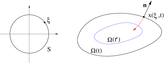
Figure 4: At each time $t\in[0,T]$, the boundary of the set $\Omega(t)$ is parameterized by $\xi\mapsto x(t,\xi)$, where $\xi\in S$ ranges over the unit circle.

We are now ready to state our main result, providing necessary conditions for optimality.

Theorem 5.1

Let $E$ satisfy (A1) and let $\phi:I\!\!R_{+}\mapsto I\!\!R_{+}$ be a ${\cal C}^{1}$ function which satisfies (A2). Assume that $t\mapsto\Omega(t)$ provides an optimal solution to (OP). Let $\xi\mapsto x(t,\xi)$ be a ${\cal C}^{2}$ parameterization of the boundary of the set $\Omega(t)$, satisfying (A3). Let $\lambda(t)$ be as in (5.6) and consider the adjoint function $Y=Y(t,\xi)$ constructed at (5.4)-(5.5).

Then, for every $t\in[0,T]$ and $\xi\in S$, the normal velocity $\beta=\beta(t,\xi)$ satisfies

$$\lambda(t)E\big{(}\beta(t,\xi)\bigr{)}-Y(t,\xi)\beta(t,\xi)~{}=~{}\min_{\beta\geq\beta_{0}}~{}\Big{\{}\lambda(t)E(\beta)-Y(t,\xi)\beta\Big{\}}.$$ (5.7)

Proof. 1. Assume that the conclusion fails. We can thus find a point $(\tau,\xi_{0})\in]0,T[\,\times S$ and some value $\overline{\beta}\in I\!\!R$ such that

$$\lambda(\tau)E\big{(}\beta(\tau,\xi_{0})\bigr{)}-Y(\tau,\xi_{0})\beta(\tau,\xi_{0})~{}>~{}\lambda(\tau)E(\overline{\beta})-Y(\tau,\xi_{0})\overline{\beta}.$$ (5.8)

We shall construct a family of perturbations $\Omega^{\varepsilon}(t)$, $t\in[0,T]$, which achieve a lower cost. Here $\Omega^{\varepsilon}(t)$ will be the set with boundary

$$\partial\Omega^{\varepsilon}(t)~{}=~{}\bigl{\{}x^{\varepsilon}(t,\xi)\,;~{}\xi\in S\bigr{\}},$$ (5.9)

for suitable perturbations $x^{\varepsilon}$ (see Fig. 6). These resemble the “needle variations” used in the classical proof of the Pontryagin maximum principle. Namely, we perform a large change in the inward normal velocity $\beta=\beta(t,\xi)$ (which here plays the role of a control function) on the small domain $[\tau-\varepsilon^{4},\tau]\times[\xi_{0}-\varepsilon,\xi_{0}+\varepsilon]$. At all subsequent times $t\in[\tau,T]$, we choose the perturbed normal velocity $\beta^{\varepsilon}$ so that its cost remains almost the same as is the original solution. 2. As a preliminary, consider a smooth function $\varphi:I\!\!R\mapsto[0,1]$ such that

$$\left\{\begin{array}[]{rl}\varphi(s)=1&\hbox{if}~{}~{}s\leq 0,\cr\varphi(s)=0&\hbox{if}~{}~{}s\geq 1,\cr\varphi^{\prime}(s)\leq 0&\hbox{for all}~{}~{}s\in I\!\!R.\end{array}\right.$$

As shown in Fig. 5, we then define the functions

$$\varphi_{\varepsilon}(s)~{}\doteq~{}\varphi\left({|s|-\varepsilon\over\varepsilon^{2}}\right).$$ (5.10)

Recalling (5.3), for $t\in[\tau,T]$ we define $X=X(t,\xi)$ to be the solution to the linearized evolution equation

$$X_{t}(t,\xi)~{}=~{}{E\bigl{(}\beta(t,\xi)\bigr{)}\over E^{\prime}\bigl{(}\beta(t,\xi)\bigr{)}}\cdot\omega(t,\xi)\,X(t,\xi),$$ (5.11)

with initial data at $t=\tau$ given by

$$X(\tau,\xi)~{}=~{}\bigl{[}\overline{\beta}-\beta(\tau,\xi_{0})\bigr{]}\cdot\varphi_{\varepsilon}(\xi-\xi_{0}).$$ (5.12)

Figure 5: The functions $\varphi_{\varepsilon}$ introduced at (5.10).

The perturbations $x^{\varepsilon}$ are now defined as follows. On an initial time interval, we set

$$x^{\varepsilon}(t,\xi)~{}=~{}x(t,\xi)\qquad\hbox{if}\quad t\in[0,\tau-\varepsilon^{4}],~{}\xi\in S.$$ (5.13)

For $t\geq\tau$, recalling (5.11)-(5.12), we define

$$x^{\varepsilon}(t,\xi)~{}=~{}x(t,\xi)+\varepsilon^{4}X(t,\xi){\bf n}(t,\xi)\qquad\hbox{if}\quad t\in[\tau,T],~{}\xi\in S.$$ (5.14)

Finally, in the remaining small interval of time before $\tau$, we define $x^{\varepsilon}$ by setting

$$x^{\varepsilon}(t,\xi)~{}=~{}x(t,\xi)+\bigl{[}\varepsilon^{4}-(\tau-t)\bigr{]}\,X(\tau,\xi){\bf n}(t,\xi)\qquad\hbox{if}\quad t\in[\tau-\varepsilon^{4},\,\tau],~{}\xi\in S.$$ (5.15)

In the remainder of the proof we will show that, if (5.8) holds, then for a suitably small $\varepsilon>0$ the perturbed sets $\Omega^{\varepsilon}(t)$ in (5.9) achieve a strictly smaller cost. In view of the definition of the perturbation $X$, it will be convenient to split the domain as

$$S~{}=~{}S_{1}\cup S_{2}\cup S_{3}\,,$$ (5.16)

where

$$\begin{array}[]{rl}S_{1}&\doteq~{}\bigl{\{}\xi\in S\,;~{}|\xi-\xi_{0}|\leq\varepsilon\bigr{\}},\\[5.69054pt] S_{2}&\doteq~{}\bigl{\{}\xi\in S\,;~{}\varepsilon<|\xi-\xi_{0}|<\varepsilon+\varepsilon^{2}\bigr{\}},\\[5.69054pt] S_{3}&\doteq~{}\bigl{\{}\xi\in S\,;~{}|\xi-\xi_{0}|\geq\varepsilon+\varepsilon^{2}\bigr{\}}.\end{array}$$ (5.17)

3. We begin by analyzing what happens during the interval $[\tau-\varepsilon^{4},\tau]$, where, by (5.12) and (5.15),

$$x^{\varepsilon}(t,\xi)~{}=~{}x(t,\xi)+\bigl{[}\varepsilon^{4}-(\tau-t)\bigr{]}\,\bigl{[}\overline{\beta}-\beta(\tau,\xi_{0})\bigr{]}\cdot\varphi_{\varepsilon}(\xi-\xi_{0}){\bf n}(t,\xi).$$ (5.18)

Differentiating w.r.t. $\xi$ and recalling (5.10), we obtain

$$\begin{array}[]{rl}x^{\varepsilon}_{\xi}(t,\xi)&=~{}x_{\xi}(t,\xi)+\bigl{[}\varepsilon^{4}-(\tau-t)\bigr{]}\,\bigl{[}\overline{\beta}-\beta(\tau,\xi_{0})\bigr{]}\cdot\varphi^{\prime}_{\varepsilon}(\xi-\xi_{0}){\bf n}(t,\xi)\\[8.53581pt] &\qquad+\bigl{[}\varepsilon^{4}-(\tau-t)\bigr{]}\,\bigl{[}\overline{\beta}-\beta(\tau,\xi_{0})\bigr{]}\cdot\varphi_{\varepsilon}(\xi-\xi_{0}){\bf n}_{\xi}(t,\xi).\end{array}$$ (5.19)

In connection with the decomposition (5.16)-(5.17), by (5.12), we have

$$x^{\varepsilon}_{\xi}(t,\xi)-x_{\xi}(t,\xi)~{}=~{}\left\{\begin{array}[]{cl}{\cal O}(1)\cdot\varepsilon^{4}&\hbox{if}\quad\xi\in S_{1}\,,\\[2.84526pt] {\cal O}(1)\cdot\varepsilon^{2}&\hbox{if}\quad\xi\in S_{2}\,,\\[2.84526pt] 0&\hbox{if}\quad\xi\in S_{3}\,.\end{array}\right.$$ (5.20)

In view of (5.1), the same bounds hold for the normal vector ${\bf n}^{\varepsilon}(t,\xi)$, namely

$${\bf n}^{\varepsilon}(t,\xi)-{\bf n}(t,\xi)~{}=~{}\left\{\begin{array}[]{cl}{\cal O}(1)\cdot\varepsilon^{4}&\hbox{if}\quad\xi\in S_{1}\,,\\[2.84526pt] {\cal O}(1)\cdot\varepsilon^{2}&\hbox{if}\quad\xi\in S_{2}\,,\\[2.84526pt] 0&\hbox{if}\quad\xi\in S_{3}\,.\end{array}\right.$$ (5.21)

Next, differentiating (5.18) w.r.t. time, we compute

$$\begin{array}[]{rl}\beta^{\varepsilon}(t,\xi)&=~{}\big{\langle}x^{\varepsilon}_{t}(t,\xi)\,,~{}{\bf n}^{\varepsilon}(t,\xi)\big{\rangle}\\[8.53581pt] &=~{}\Big{\langle}\beta(t,\xi){\bf n}(t,\xi)+\bigl{[}\overline{\beta}-\beta(\tau,\xi_{0})\bigr{]}\cdot\varphi_{\varepsilon}(\xi-\xi_{0}){\bf n}(t,\xi),\,{\bf n}^{\varepsilon}(t,\xi)\Big{\rangle}\\[8.53581pt] &\qquad\qquad+~{}\Big{\langle}\bigl{[}\varepsilon^{4}-(\tau-t)\bigr{]}\,\bigl{[}\overline{\beta}-\beta(\tau,\xi_{0})\bigr{]}\cdot\varphi_{\varepsilon}(\xi-\xi_{0}){\bf n}_{t}(t,\xi),\,{\bf n}^{\varepsilon}(t,\xi)\Big{\rangle}\\[8.53581pt] &=\displaystyle~{}\beta(t,\xi)+\Big{\langle}\beta(t,\xi){\bf n}(t,\xi),\,{\bf n}^{\varepsilon}(t,\xi)-{\bf n}(t,\xi)\Big{\rangle}\\[8.53581pt] &\qquad\qquad\displaystyle+\bigl{[}\overline{\beta}-\beta(\tau,\xi_{0})\bigr{]}\varphi_{\varepsilon}(\xi-\xi_{0})]\Big{(}1+\big{\langle}{\bf n}(t,\xi),\,{\bf n}^{\varepsilon}(t,\xi)-{\bf n}(t,\xi)\big{\rangle}\Big{)}\\[8.53581pt] &\displaystyle\qquad\qquad+\bigl{[}\varepsilon^{4}-(\tau-t)\bigr{]}\,\bigl{[}\overline{\beta}-\beta(\tau,\xi_{0})\bigr{]}\varphi_{\varepsilon}(\xi-\xi_{0})\cdot\big{\langle}{\bf n}_{t}(t,\xi),\,{\bf n}^{\varepsilon}(t,\xi)-{\bf n}(t,\xi)\big{\rangle}.\end{array}$$ (5.22)

We here used the fact that $\langle{\bf n}_{t},{\bf n}\rangle=0$, because ${\bf n}$ is a unit vector. In view of (5.21), we conclude

$$\beta^{\varepsilon}(t,\xi)-\beta(t,\xi)~{}=~{}\left\{\begin{array}[]{cl}\overline{\beta}-\beta(\tau,\xi_{0})+{\cal O}(1)\cdot\varepsilon&\hbox{if}\quad\xi\in S_{1}\,,\\[2.84526pt] {\cal O}(1)&\hbox{if}\quad\xi\in S_{2}\,,\\[2.84526pt] 0&\hbox{if}\quad\xi\in S_{3}\,.\end{array}\right.$$ (5.23)

For $t\in[\tau-\varepsilon^{4},\tau]$, by (5.20) and (5.23) we obtain

$$\begin{array}[]{rl}{\cal E}^{\varepsilon}(t)-{\cal E}(t)&\displaystyle=~{}\int_{S}\Big{[}E\bigl{(}\beta^{\varepsilon}(t,\xi)\bigr{)}\,\bigl{|}x^{\varepsilon}_{\xi}(t,\xi)\bigr{|}-E\bigl{(}\beta(t,\xi)\bigr{)}\,\bigl{|}x_{\xi}(t,\xi)\bigr{|}\Big{]}\,d\xi\\[11.38109pt] &\displaystyle=~{}\int_{|\xi-\xi_{0}|<\varepsilon}\bigl{[}E(\overline{\beta})-E(\beta(\tau,\xi_{0})\bigr{]}\,\bigl{|}x_{\xi}(\tau,\xi_{0})\bigr{|}\,d\xi+{\cal O}(1)\cdot\varepsilon^{2}\\[11.38109pt] &=~{}2\varepsilon\,\bigl{[}E(\overline{\beta})-E(\beta(\tau,\xi_{0})\bigr{]}\,\bigl{|}x_{\xi}(\tau,\xi_{0})\bigr{|}+{\cal O}(1)\cdot\varepsilon^{2}.\end{array}$$ (5.24)

Integrating over time, we finally obtain

$$\int_{\tau-\varepsilon^{4}}^{\tau}\Big{[}\phi\bigl{(}{\cal E}^{\varepsilon}(t)\bigr{)}-\phi\bigl{(}{\cal E}(t)\bigr{)}\Big{]}\,dt~{}=~{}\phi^{\prime}\bigl{(}{\cal E}(\tau)\bigr{)}\cdot 2\varepsilon^{5}\bigl{[}E(\overline{\beta})-E(\beta(\tau,\xi_{0})\bigr{]}\,\bigl{|}x_{\xi}(\tau,\xi_{0})\bigr{|}+{\cal O}(1)\cdot\varepsilon^{6}.$$ (5.25)

4. In this step we compute the difference ${\cal E}^{\varepsilon}(t)-{\cal E}(t)$ in the control effort, during the time interval $t\in[\tau,T]$. For $(t,\xi)\in[\tau,T]\times S$, the solution $X$ of (5.11)-(5.12) will satisfy different bounds over the above three sets:

$$X_{\xi}(t,\xi)~{}=~{}\left\{\begin{array}[]{cl}\quad{\cal O}(1)&\hbox{if}\quad\xi\in S_{1}\,,\\ {\cal O}(1)\cdot\varepsilon^{-2}&\hbox{if}\quad\xi\in S_{2}\,,\\ \quad 0&\hbox{if}\quad\xi\in S_{3}\,.\end{array}\right.$$ (5.26)

Therefore

$$x^{\varepsilon}_{\xi}(t,\xi)-x_{\xi}(t,\xi)~{}=~{}\begin{cases}{\cal O}(1)\cdot\varepsilon^{4}\quad&\hbox{if}\quad\xi\in S_{1}\,,\\ {\cal O}(1)\cdot\varepsilon^{2}\quad&\hbox{if}\quad\xi\in S_{2}\,,\\ \quad 0\quad\quad&\hbox{if}\quad\xi\in S_{3}\,.\end{cases}$$ (5.27)

The change in the normal speed is computed by

$$\begin{array}[]{rl}\beta^{\varepsilon}-\beta&=~{}\big{\langle}x^{\varepsilon}_{t},\,{\bf n}^{\varepsilon}\big{\rangle}-\big{\langle}x_{t},\,{\bf n}\big{\rangle}\\[8.53581pt] &=~{}\varepsilon^{4}X_{t}+\Big{\langle}\beta{\bf n}+\varepsilon^{4}X_{t}{\bf n}+\varepsilon^{4}X{\bf n}_{t}\,,~{}{\bf n}^{\varepsilon}-{\bf n}\Big{\rangle}.\end{array}$$ (5.28)

We observe that ${\bf n}^{\varepsilon}$ and ${\bf n}$ are unit vectors. For $\xi\in S_{1}$, by (5.21) the angle between them is

$$\theta_{\varepsilon}~{}=~{}{\cal O}(1)\cdot|{\bf n}^{\varepsilon}-{\bf n}|~{}=~{}{\cal O}(1)\cdot\varepsilon^{4}.$$

Therefore,

$$\big{\langle}{\bf n},\,{\bf n}^{\varepsilon}-{\bf n}\big{\rangle}~{}=~{}\cos\theta_{\varepsilon}-1~{}=~{}{\cal O}(1)\cdot\theta_{\varepsilon}^{2}~{}=~{}{\cal O}(1)\cdot\varepsilon^{8}.$$ (5.29)

Similarly, when $\xi\in S_{2}$, by (5.21) it follows

$$\big{\langle}{\bf n},\,{\bf n}^{\varepsilon}-{\bf n}\big{\rangle}~{}=~{}{\cal O}(1)\cdot\varepsilon^{4}.$$ (5.30)

Combining (5.28) with (5.29)-(5.30), one obtains the bounds

$$R(t,\xi)~{}\doteq~{}\beta^{\varepsilon}(t,\xi)-\beta(t,\xi)-\varepsilon^{4}X_{t}(t,\xi)~{}=~{}\left\{\begin{array}[]{cl}{\cal O}(1)\cdot\varepsilon^{8}&\hbox{if}\quad\xi\in S_{1}\,,\\ {\cal O}(1)\cdot\varepsilon^{4}&\hbox{if}\quad\xi\in S_{2}\,,\\ 0&\hbox{if}\quad\xi\in S_{3}\,.\end{array}\right.$$ (5.31)

We now compute

$$\begin{array}[]{rl}\bigl{|}x^{\varepsilon}_{\xi}\bigr{|}-|x_{\xi}|&=\displaystyle~{}\Big{\langle}(x+\varepsilon^{4}X{\bf n})_{\xi}\,,~{}(x+\varepsilon^{4}X{\bf n})_{\xi}\Big{\rangle}^{1/2}-|x_{\xi}|\\[8.53581pt] &\displaystyle=~{}\varepsilon^{4}\,\left\langle{x_{\xi}\over|x_{\xi}|}\,,~{}X_{\xi}{\bf n}+X{\bf n}_{\xi}\right\rangle+{\cal O}(1)\cdot\varepsilon^{8}\\[11.38109pt] &=~{}\displaystyle-\varepsilon^{4}\big{\langle}{\bf n}^{\perp},{\bf n}_{\xi}\big{\rangle}X+{\cal O}(1)\cdot\varepsilon^{8}\\[11.38109pt] &=~{}-\varepsilon^{4}\omega|x_{\xi}|\,X+{\cal O}(1)\cdot\varepsilon^{8}\,,\end{array}$$ (5.32)

where $\omega$ denotes the signed curvature, as in (5.3).

Combining (5.32) with the evolution equation (5.11) for the perturbation $X$, and using (5.31), we obtain

$$\begin{array}[]{l}E(\beta^{\varepsilon})\,|x^{\varepsilon}_{\xi}|-E(\beta)\,|x_{\xi}|\\[11.38109pt] \qquad=~{}\Big{[}E(\beta^{\varepsilon})-E(\beta)\bigr{]}\,|x_{\xi}|+E(\beta)\,\big{(}|x^{\varepsilon}_{\xi}|-|x_{\xi}|\bigr{)}+\Big{[}E(\beta^{\varepsilon})-E(\beta)\bigr{]}\,\big{(}|x^{\varepsilon}_{\xi}|-|x_{\xi}|\bigr{)}\\[11.38109pt] \qquad=~{}E^{\prime}(\beta)[\beta^{\varepsilon}-\beta]\,|x_{\xi}|+{\cal O}(1)\cdot|\beta^{\varepsilon}-\beta|^{2}+E(\beta)\,\big{(}|x^{\varepsilon}_{\xi}|-|x_{\xi}|\bigr{)}+{\cal O}(1)\cdot|\beta^{\varepsilon}-\beta|\,\big{(}|x^{\varepsilon}_{\xi}|-|x_{\xi}|\bigr{)}\\[11.38109pt] \qquad=~{}E^{\prime}(\beta)(\varepsilon^{4}X_{t}+R)\,|x_{\xi}|+{\cal O}(1)\cdot|\beta^{\varepsilon}-\beta|^{2}+E(\beta)\,\big{(}-\varepsilon\omega|x_{\xi}|X+{\cal O}(1)\cdot\varepsilon^{8}\bigr{)}\\[11.38109pt] \qquad\qquad+{\cal O}(1)\cdot|\beta^{\varepsilon}-\beta|\,\big{(}|x^{\varepsilon}_{\xi}|-|x_{\xi}|\bigr{)},\end{array}$$ (5.33)

$$E\bigl{(}\beta^{\varepsilon}(t,\xi)\bigr{)}\,\bigl{|}x^{\varepsilon}_{\xi}(t,\xi)\bigr{|}-E\bigl{(}\beta(t,\xi)\bigr{)}\bigl{|}x_{\xi}(t,\xi)\bigr{|}~{}=~{}\left\{\begin{array}[]{cl}{\cal O}(1)\cdot\varepsilon^{8}&\hbox{if}\quad\xi\in S_{1}\,,\\ {\cal O}(1)\cdot\varepsilon^{4}&\hbox{if}\quad\xi\in S_{2}\,,\\ 0&\hbox{if}\quad\xi\in S_{3}\,.\end{array}\right.$$ (5.34)

Integrating over the whole set $S$, for every $t\in[\tau,T]$ we thus obtain

$${\cal E}^{\varepsilon}(t)-{\cal E}(t)~{}=~{}{\cal O}(1)\cdot\varepsilon^{8}\,\hbox{meas}(S_{1})+{\cal O}(1)\cdot\varepsilon^{4}\,\hbox{meas}(S_{2})~{}=~{}{\cal O}(1)\cdot\varepsilon^{6},$$ (5.35)

and finally

$$\int_{\tau}^{T}\bigl{[}{\cal E}^{\varepsilon}(t)-{\cal E}(t)\bigr{]}\,dt~{}=~{}{\cal O}(1)\cdot\varepsilon^{6}.$$ (5.36)

In other words, by the identity (5.11) and the choice of the function $x^{\varepsilon}$ in (5.14), the change in the cost of the control $\beta$ over the remaining time interval $[\tau,T]$ vanishes, to higher order. 5. It remains to estimate the change in the running cost and in the terminal cost for the perturbed strategies. We compute

$$\begin{array}[]{l}\displaystyle\left(\int_{\tau-\varepsilon^{4}}^{\tau}+\int_{\tau}^{T}\right)\Big{[}m_{2}\bigl{(}\Omega^{\varepsilon}(t)\bigr{)}-m_{2}\bigl{(}\Omega(t)\bigr{)}\Big{]}\,dt\\[11.38109pt] \displaystyle\qquad=~{}{\cal O}(1)\cdot\varepsilon^{9}-\int_{\tau}^{T}\int_{S_{1}\cup S_{2}}\Big{(}\varepsilon^{4}X(t,\xi)+{\cal O}(1)\cdot\varepsilon^{5}\Big{)}\,\bigl{|}x_{\xi}(t,\xi)\bigr{|}\,d\xi\,dt\\[11.38109pt] \displaystyle\qquad=~{}-\varepsilon^{4}\int_{\tau}^{T}\int_{S_{1}}X(t,\xi)\,\bigl{|}x_{\xi}(t,\xi)\bigr{|}\,d\xi\,dt+{\cal O}(1)\cdot\varepsilon^{6}.\end{array}$$ (5.37)

Moreover, the change in the final area can be estimated as

$$\begin{array}[]{l}\displaystyle m_{2}\bigl{(}\Omega^{\varepsilon}(T)\bigr{)}-m_{2}\bigl{(}\Omega(T)\bigr{)}~{}=~{}-\int_{S_{1}\cup S_{2}}\Big{(}\varepsilon^{4}X(T,\xi)+{\cal O}(1)\cdot\varepsilon^{5}\Big{)}\,\bigl{|}x_{\xi}(T,\xi)\bigr{|}\,d\xi\\[11.38109pt] \qquad\displaystyle=~{}-\varepsilon^{4}\int_{\tau}^{T}\int_{S_{1}}X(T,\xi)\,\bigl{|}x_{\xi}(T,\xi)\bigr{|}\,d\xi\,dt+{\cal O}(1)\cdot\varepsilon^{6}.\end{array}$$ (5.38)

We now claim that, if the adjoint variable $Y$ satisfies (5.4)-(5.5), then the change in cost can be computed by

$$c_{1}\int_{\tau}^{T}\int_{S_{1}}\bigl{|}x_{\xi}(t,\xi)\bigr{|}X(t,\xi)\,d\xi dt+c_{2}\int_{S_{1}}\bigl{|}x_{\xi}(T,\xi)\bigr{|}X(T,\xi)\,d\xi~{}=~{}\int_{S_{1}}\bigl{|}x_{\xi}(\tau,\xi)\bigr{|}X(\tau,\xi)\,Y(\tau,\xi)\,d\xi.$$ (5.39)

Indeed, this is trivially true when $\tau=T$, because in this case $Y(T,\xi)=c_{2}$. Moreover, differentiating (5.39) w.r.t. time $\tau$, by (5.11) and (5.4) we obtain

$$\begin{array}[]{l}\displaystyle{d\over d\tau}\int_{S_{1}}\bigl{|}x_{\xi}(\tau,\xi)\bigr{|}\,X(\tau,\xi)\,Y(\tau,\xi)\,d\xi\\[11.38109pt] \qquad\displaystyle=~{}\int_{S_{1}}\left(-\omega(\tau,\xi)\,\beta(\tau,\xi)+{E\bigl{(}\beta(\tau,\xi)\bigr{)}\over E^{\prime}\bigl{(}\beta(\tau,\xi)\bigr{)}}\cdot\omega(\tau,\xi)\right)\bigl{|}x_{\xi}(\tau,\xi)\bigr{|}X(\tau,\xi)\,Y(\tau,\xi)\,d\xi\\[11.38109pt] \qquad\qquad\displaystyle+\int_{S_{1}}\bigl{|}x_{\xi}(\tau,\xi)\bigr{|}X(\tau,\xi)\,Y_{\tau}(\tau,\xi)\,d\xi\\[11.38109pt] \qquad\displaystyle=~{}-c_{1}\int_{S_{1}}\bigl{|}x_{\xi}(\tau,\xi)\bigr{|}X(\tau,\xi)\,d\xi~{}=~{}{d\over d\tau}\int_{\tau}^{T}\int_{S_{1}}c_{1}\bigl{|}x_{\xi}(t,\xi)\bigr{|}X(t,\xi)\,d\xi dt\,.\end{array}$$ (5.40)

This shows that the identity (5.39) holds for every $\tau$.

Together with (5.37)-(5.38), from (5.39) we obtain

$$\begin{array}[]{l}\displaystyle c_{1}\,\left(\int_{\tau-\varepsilon^{4}}^{\tau}+\int_{\tau}^{T}\right)\Big{[}m_{2}\bigl{(}\Omega^{\varepsilon}(t)\bigr{)}-m_{2}\bigl{(}\Omega(t)\bigr{)}\Big{]}\,dt+c_{2}\,m_{2}\bigl{(}\Omega^{\varepsilon}(T)\bigr{)}-m_{2}\bigl{(}\Omega(T)\bigr{)}\\[11.38109pt] \qquad=~{}\displaystyle-\varepsilon^{4}\,\int_{S_{1}}\bigl{|}x_{\xi}(\tau,\xi)\bigr{|}\,X(\tau,\xi)\,Y(\tau,\xi)\,d\xi+{\cal O}(1)\cdot\varepsilon^{6}\\[11.38109pt] \qquad=~{}-2\varepsilon^{5}\bigl{|}x_{\xi}(\tau,\xi_{0})\bigr{|}\,X(\tau,\xi_{0})\,Y(\tau,\xi_{0})+{\cal O}(1)\cdot\varepsilon^{6}\\[11.38109pt] \qquad=~{}-2\varepsilon^{5}\bigl{|}x_{\xi}(\tau,\xi_{0})\bigr{|}\,\bigl{(}\overline{\beta}-\beta(\tau,\xi_{0})\bigr{)}Y(\tau,\xi_{0})+{\cal O}(1)\cdot\varepsilon^{6}\par\end{array}$$ (5.41)

6. By assumption, the cost of the perturbation cannot be lower than the original cost. In view of (5.25), (5.36), and (5.41), this implies

$$\phi^{\prime}\bigl{(}{\cal E}(\tau)\bigr{)}\cdot 2\varepsilon^{5}\bigl{[}E(\overline{\beta})-E(\beta(\tau,\xi_{0})\bigr{]}\,\bigl{|}x_{\xi}(\tau,\xi_{0})\bigr{|}-2\varepsilon^{5}\bigl{|}x_{\xi}(\tau,\xi_{0})\bigr{|}\,\,\bigl{(}\overline{\beta}-\beta(\tau,\xi_{0})\bigr{)}Y(\tau,\xi_{0})+{\cal O}(1)\cdot\varepsilon^{6}~{}\geq~{}0$$ (5.42)

for every $(\tau,\xi)\in\,]0,T[\,\times S$ and every speed $\overline{\beta}\geq\beta_{0}$. Since $\varepsilon>0$ can be taken arbitrarily small, from (5.42) we deduce

$$\phi^{\prime}\bigl{(}{\cal E}(\tau)\bigr{)}\bigl{[}E(\overline{\beta})-E(\beta(\tau,\xi_{0})\bigr{]}-\bigl{(}\overline{\beta}-\beta(\tau,\xi_{0})\bigr{)}Y(\tau,\xi_{0})~{}\geq~{}0$$ (5.43)

for every $\overline{\beta}\geq\beta_{0}$. This proves (5.7).

Finally, by continuity the same conclusion remains valid also for $t=0$ or $t=T$. MM     

Figure 6: A perturbation of the optimal strategy. If at time $\tau$ the additional region $\widehat{\Omega}$ could be freed from the contamination, the total cost would be reduced in the amount $m_{2}(\widehat{\Omega})\cdot Y(\tau,\xi_{0})$.

Remark 5.1

The adjoint variable $Y>0$ introduced at (5.4)-(5.5) can be interpreted as a “shadow price”. Namely (see Fig. 6), assume that at time $\tau$ an external contractor offered to remove the contamination from a neighborhood of the point $x(\tau,\xi_{0})$, thus replacing the set $\Omega(\tau)$ with a smaller set $\Omega^{\varepsilon}(\tau)$, at a price of $Y(\tau,\xi_{0})$ per unit area. In this case, accepting or refusing the offer would make no difference in the total cost.

Remark 5.2

In order to derive the necessary conditions (5.7), we assumed that the parameterization $(t,\xi)\mapsto x(t,\xi)$ had ${\cal C}^{2}$ regularity. In several applications, this map is continuously differentiable, but only piecewise ${\cal C}^{2}$. In particular (see the example in Section 8), the curvature $\omega(t,\xi)$ may only be piecewise continuous. It is worth noting that the proof of Theorem 5.1 remains valid also in this slightly more general setting.

6 The case with constraint on the total effort

We now consider again the optimization problem (OP), but in the case where the cost function $\phi$ is given by (1.9). This is equivalent to an optimization problem with constraint on the total effort:

$$\hbox{minimize:}\qquad{\cal J}(\Omega)~{}=~{}c_{1}\int_{0}^{T}m_{2}(\Omega(t))\,dt+c_{2}\,\hbox{meas}\bigl{(}\Omega(T)\bigr{)},$$ (6.1)

subject to

$${\cal E}(t)~{}\doteq~{}\int_{\partial\Omega(t)}E(\beta(t,x))\,d\sigma~{}\leq~{}M\qquad\hbox{ for every}~{}~{}~{}t\in[0,T].$$ (6.2)

This leads to a somewhat different set of necessary conditions.

Theorem 6.1

Let $E$ satisfy the assumptions (A1). Assume that $t\mapsto\Omega(t)$ provides an optimal solution to (6.1)-(6.2). Let $\xi\mapsto x(t,\xi)$ be a ${\cal C}^{2}$ parameterization of the boundary of the set $\Omega(t)$, satisfying the regularity properties (A3). Call $Y=Y(t,\xi)$ the adjoint function constructed at (5.4)-(5.5).

Then, for every $t\in[0,T]$ one has ${\cal E}(t)=M$. Moreover, there exists a scalar function $t\mapsto\lambda(t)>0$ such that the normal velocity $\beta=\beta(t,\xi)$ satisfies

$$\lambda(t)E\big{(}\beta(t,\xi)\bigr{)}-Y(t,\xi)\beta(t,\xi)~{}=~{}\min_{\beta\geq\beta_{0}}~{}\Big{\{}\lambda(t)E(\beta)-Y(t,\xi)\beta\Big{\}}.$$ (6.3)

Proof. 1. To prove the first statement, we argue by contradiction. If ${\cal E}(\tau)<M$, by continuity we can assume ${\cal E}(t)<M$ for all $t$ in a neighborhood of $\tau$. Then we can choose any $\xi_{0}\in S$ and any constant $\overline{\beta}>\beta(\tau,\xi_{0})$. For $\varepsilon>0$ small, we define the perturbed strategy $x^{\varepsilon}$ on $[\tau-\varepsilon^{4},\tau]$ as in (5.12), (5.15). Since we are changing the inward velocity $\beta$ only when $|\xi-\xi_{0}|<\varepsilon+\varepsilon^{2}$, for $\varepsilon>0$ small enough the corresponding total effort will satisfy

$${\cal E}^{\varepsilon}(t)~{}\leq~{}{\cal E}(t)+C\,\varepsilon~{}<~{}M\qquad\hbox{for all}~{}t\in[\tau-\varepsilon^{4},\tau].$$

Notice that this perturbation satisfies

$$\Omega^{\varepsilon}(t)\subseteq\Omega(t)\qquad\hbox{for all}~{}t\in[0,\tau].$$

Moreover, the inclusion is strict for $\tau-\varepsilon<t\leq\tau$.

For $t\in[\tau,T]$ we now define

$$\Omega^{\varepsilon}(t)~{}=~{}\Omega(t)\cap B\Big{(}\Omega^{\varepsilon}(\tau),|\beta_{0}|(t-\tau)\Big{)}.$$

This yields

$${\cal E}^{\varepsilon}(t)~{}\leq~{}{\cal E}(t)~{}\leq~{}M\qquad\hbox{for all}~{}t\in[\tau,T].$$ (6.4)

Indeed, at a.e. boundary point $x\in\partial\Omega^{\varepsilon}(t)$, two cases can arise:

• $x\in\partial\Omega^{\varepsilon}(t)\cap\partial\Omega(t)$. Then the inward normal speed at $x$ is the same as in the original solution.

• $x\in\partial\Omega^{\varepsilon}(t)\setminus\partial\Omega(t)$, so that

  $$d\bigl{(}x\,;~{}\Omega^{\varepsilon}(\tau)\bigr{)}~{}=~{}|\beta_{0}|(t-\tau).$$

  In this case, the inward normal speed is precisely $\beta_{0}$, and this comes at zero cost.

Combining the two above cases, we obtain (6.4).

In conclusion, we obtained an admissible motion $t\mapsto\Omega^{\varepsilon}(t)\subseteq\Omega(t)$, which achieves the strict inequality

$$\int_{\tau-\varepsilon^{4}}^{\tau}\Omega^{\varepsilon}(t)\,dt~{}<~{}\int_{\tau-\varepsilon^{4}}^{\tau}\Omega(t)\,dt.$$

This contradicts the optimality of $\Omega(\cdot)$. 2. To prove the second statement, we need to find $\lambda(t)>0$ for which the (6.3) holds.

Fix a time $\tau$, and consider any two points $\xi_{1},\xi_{2}\in S$ where the control is active:

$$\beta(\tau,\xi_{1})\,>\,\beta_{0},\qquad\beta(\tau,\xi_{2})\,>\,\beta_{0}.$$

We claim that for $i=1,2$ the ratios ${Y(\tau,\xi_{i})/E^{\prime}\bigl{(}\beta(\tau,\xi_{i})\bigr{)}}$ must be equal. If they are not, assuming that

$${Y(\tau,\xi_{1})\over E^{\prime}\bigl{(}\beta(\tau,\xi_{1})\bigr{)}}~{}>~{}{Y(\tau,\xi_{2})\over E^{\prime}\bigl{(}\beta(\tau,\xi_{2})\bigr{)}}~{}>~{}0\,,$$ (6.5)

we will obtain a contradiction.

Indeed, recalling that $Y>0$, by (6.5) we deduce the existence of $\delta_{1},\delta_{2}>0$ small enough such that

$$\delta_{1}E^{\prime}(\tau,\xi_{1})~{}>~{}\delta_{2}E^{\prime}(\tau,\xi_{2}),$$ (6.6)

$$\delta_{1}Y(\tau,\xi_{1})~{}>~{}\delta_{2}Y(\tau,\xi_{2})~{}>~{}0.$$ (6.7)

Since the function $E$ is continuously differentiable, by possibly shrinking the values of $\delta_{1},\delta_{2}$ while keeping the ratio $\delta_{1}/\delta_{2}$ constant, by (6.6) we obtain

$$\begin{array}[]{l}\displaystyle\bigl{|}x_{\xi}(\tau,\xi_{1})\bigr{|}\left[E\left(\beta(\tau,\xi_{1})+{\delta_{1}\over\bigl{|}x_{\xi}(\tau,\xi_{1})\bigr{|}}\right)-E\bigl{(}\beta(\tau,\xi_{1})\bigr{)}\right]\\[11.38109pt] \qquad\displaystyle<~{}\bigl{|}x_{\xi}(\tau,\xi_{2})\bigr{|}\left[E\bigl{(}\beta(\tau,\xi_{2})\bigr{)}-E\left(\beta(\tau,\xi_{2})-{\delta_{2}\over\bigl{|}x_{\xi}(\tau,\xi_{1})\bigr{|}}\right)\right],\end{array}$$ (6.8)

For $\varepsilon>0$ small we construct a perturbation $x^{\varepsilon}(t,\xi)$ as in the proof of Theorem 5.1, but taking place simultaneously over the two disjoint intervals

$$I_{1}\cup I_{2}~{}=~{}\{\xi\,;~{}|\xi-\xi_{1}|<\varepsilon+\varepsilon^{2}\}\cup\{\xi\,;~{}|\xi-\xi_{2}|<\varepsilon+\varepsilon^{2}\}.$$

At time $\tau$ we define

$$X^{\varepsilon}(\tau,\xi)~{}=~{}{\delta_{1}\over\bigl{|}x_{\xi}(\tau,\xi_{1})\bigr{|}}\,\varphi_{\varepsilon}(\xi-\xi_{1})-{\delta_{2}\over\bigl{|}x_{\xi}(\tau,\xi_{2})\bigr{|}}\,\varphi_{\varepsilon}(\xi-\xi_{2}).$$ (6.9)

On the remaining interval $[\tau,T]$, we define $X^{\varepsilon}$ to be the solution of

$$X^{\varepsilon}_{t}(t,\xi)~{}=~{}{E\bigl{(}\beta(t,\xi)\bigr{)}\over E^{\prime}\bigl{(}\beta(t,\xi)\bigr{)}}\cdot\omega(t,\xi)\,X^{\varepsilon}(t,\xi)-\varepsilon^{2/3}\,\bigl{|}X^{\varepsilon}(t,\xi)\bigr{|},$$ (6.10)

with initial data (6.9) at $t=\tau$. Notice that, compared with (5.11)-(5.12), here the construction of $X^{\varepsilon}$ includes a further $\varepsilon$-perturbation. This is needed, in order to guarantee that the total effort remains $\leq M$ at all times.

Similarly to the proof of Theorem 5.1, for all $\xi\in S$ we now define

$$x^{\varepsilon}(t,\xi)~{}=~{}\left\{\begin{array}[]{cl}x(t,\xi)&\hbox{if}~{}~{}t\in[0,\tau-\varepsilon^{4}],\\[8.53581pt] x(t,\xi)+\bigl{[}\varepsilon^{4}-(\tau-t)\bigr{]}\,X^{\varepsilon}(\tau,\xi){\bf n}(t,\xi)&\hbox{if}\quad t\in[\tau-\varepsilon^{4},\,\tau],\\[8.53581pt] x(t,\xi)+\varepsilon^{4}X^{\varepsilon}(\tau,\xi){\bf n}(t,\xi)&\hbox{if}~{}~{}t\in[\tau,T].\end{array}\right.$$ (6.11)

3. In this step we prove that, for $\varepsilon>0$ sufficiently small and every $t\in\,]\tau-\varepsilon^{4},\tau[\,$, the instantaneous effort satisfies

$${\cal E}^{\varepsilon}(t)~{}\leq~{}{\cal E}(t)~{}\leq~{}M.$$ (6.12)

For notational convenience, define

$$S_{1}^{i}\,\doteq\,\{\xi\in S\,;~{}|\xi-\xi_{i}|\leq\varepsilon\},\qquad S_{2}^{i}\,\doteq\,\{\xi\in S\,;~{}\varepsilon<|\xi-\xi_{i}|<\varepsilon+\varepsilon^{2}\},\qquad i=1,2$$ (6.13)

As in (5.20), one has

$$x^{\varepsilon}_{\xi}(t,\xi)-x_{\xi}(t,\xi)~{}=~{}\begin{cases}{\cal O}(1)\cdot\varepsilon^{4}\quad&\hbox{if}\quad\xi\in S_{1}^{i}\,,\\ {\cal O}(1)\cdot\varepsilon^{2}\quad&\hbox{if}\quad\xi\in S_{2}^{i}\,,\\ \quad 0\quad\quad&\hbox{otherwise.}\end{cases}$$ (6.14)

As in (5.21), the same bounds hold for ${\bf n}^{\varepsilon}-{\bf n}$.

For $\tau-\varepsilon^{4}<t<\tau$, the same arguments used at (5.23) show that the inward normal velocity satisfies

$$\beta^{\varepsilon}(t,\xi)-\beta(t,\xi)~{}=~{}\left\{\begin{array}[]{cl}\displaystyle{\delta_{1}\over\bigl{|}x_{\xi}(\tau,\xi_{1})\bigr{|}}+{\cal O}(1)\cdot\varepsilon&\hbox{if}\quad\xi\in S_{1}^{1}\,,\\[11.38109pt] \displaystyle-{\delta_{2}\over\bigl{|}x_{\xi}(\tau,\xi_{2})\bigr{|}}+{\cal O}(1)\cdot\varepsilon&\hbox{if}\quad\xi\in S_{1}^{2}\,,\\[11.38109pt] {\cal O}(1)&\hbox{if}\quad\xi\in S_{2}^{1}\cup S_{2}^{2}\,,\\[5.69054pt] 0&\hbox{otherwise.}\end{array}\right.$$ (6.15)

For $\tau-\varepsilon^{4}<t<\tau$, using (6.15) and (6.8), we now compute

$$\begin{array}[]{l}{\cal E}^{\varepsilon}(t)-{\cal E}(t)~{}\displaystyle=~{}\int_{S}\Big{[}E\bigl{(}\beta^{\varepsilon}(t,\xi)\bigr{)}\,\bigl{|}x^{\varepsilon}_{\xi}(t,\xi)\bigr{|}-E\bigl{(}\beta(t,\xi)\bigr{)}\,\bigl{|}x_{\xi}(t,\xi)\bigr{|}\Big{]}\,d\xi\\[11.38109pt] \qquad\displaystyle=~{}\varepsilon\Bigg{\{}\bigl{|}x_{\xi}(\tau,\xi_{1})\bigr{|}\left[E\Big{(}\beta(\tau,\xi_{1})+{\delta_{1}\over\bigl{|}x_{\xi}(\tau,\xi_{1})\bigr{|}}\Big{)}-E\bigl{(}\beta(\tau,\xi_{1})\bigr{)}\right]\\[11.38109pt] \qquad\qquad\qquad\displaystyle-\bigl{|}x_{\xi}(\tau,\xi_{2})\bigr{|}\left[E\bigl{(}\beta(\tau,\xi_{2})\bigr{)}-E\Big{(}\beta(\tau,\xi_{2})-{\delta_{2}\over\bigl{|}x_{\xi}(\tau,\xi_{1})\bigr{|}}\Big{)}\right]\Bigg{\}}\\[11.38109pt] \qquad\quad\displaystyle+\int_{S_{1}^{1}\cup S_{1}^{2}}{\cal O}(1)\cdot\varepsilon\,d\xi+\int_{S_{2}^{1}\cup S_{2}^{2}}{\cal O}(1)\,d\xi\\[11.38109pt] \qquad<~{}0,\end{array}$$ (6.16)

provided that $\varepsilon>0$ is sufficiently small. Indeed, the first term on the right hand side of (6.16) is strictly negative, while the last two terms are of order ${\cal O}(1)\cdot\varepsilon^{2}$. 4. Next, we estimate the change in the control effort ${\cal E}(t)$ for $\tau<t<T$. Here the computations are very similar to the ones in step 4 of the proof of Theorem 5.1. Because of the additional term on the right hand side of (6.10), the bounds (5.31) are now replaced by

$$R(t,\xi)~{}\doteq~{}\beta^{\varepsilon}(t,\xi)-\beta(t,\xi)-\varepsilon^{4}X_{t}(t,\xi)~{}=~{}\left\{\begin{array}[]{cl}{\cal O}(1)\cdot\varepsilon^{8}-\varepsilon^{4}\varepsilon^{2/3}\bigl{|}X(t,\xi)\bigr{|}&\hbox{if}\quad\xi\in S_{1}^{1}\cup S_{1}^{2}\,,\\ {\cal O}(1)\cdot\varepsilon^{4}&\hbox{if}\quad\xi\in S_{2}^{1}\cup S_{2}^{2}\,,\\ 0&\hbox{otherwise.}\end{array}\right.$$ (6.17)

In turn, the estimates (5.34) are replaced by

$$\begin{array}[]{l}E\bigl{(}\beta^{\varepsilon}(t,\xi)\bigr{)}\,\bigl{|}x^{\varepsilon}_{\xi}(t,\xi)\bigr{|}-E\bigl{(}\beta(t,\xi)\bigr{)}\bigl{|}x_{\xi}(t,\xi)\bigr{|}\\[11.38109pt] \displaystyle\qquad=~{}\left\{\begin{array}[]{cl}-\varepsilon^{4}\varepsilon^{2/3}\bigl{|}X(t,\xi)\bigr{|}E^{\prime}\bigl{(}\beta(t,\xi)\bigr{)}+{\cal O}(1)\cdot\varepsilon^{8}&\hbox{if}\quad\xi\in S_{1}^{1}\cup S_{1}^{2}\,,\\ {\cal O}(1)\cdot\varepsilon^{4}&\hbox{if}\quad\xi\in S_{2}^{1}\cup S_{2}^{2}\,,\\ 0&\hbox{otherwise.}\end{array}\right.\end{array}$$ (6.18)

We now integrate over the whole set $S$. Observing that, for $\varepsilon>0$ small, the function $|X(t,\xi)\bigr{|}$ remains uniformly positive over the set $(S_{1}^{1}\cup S_{1}^{2})\times[\tau,T]$, for a suitable constant $c_{0}>0$ and all $\tau<t<T$ we obtain

$$\begin{array}[]{rl}{\cal E}^{\varepsilon}(t)-{\cal E}(t)&\displaystyle=~{}-\int_{S_{1}^{1}\cup S_{1}^{2}}\varepsilon^{4}\varepsilon^{2/3}\bigl{|}X(t,\xi)\bigr{|}E^{\prime}\bigl{(}\beta(t,\xi)\bigr{)}\,d\xi\\[11.38109pt] &\qquad+{\cal O}(1)\cdot\varepsilon^{8}\,\hbox{meas}(S_{1}^{1}\cup S_{1}^{2})+{\cal O}(1)\cdot\varepsilon^{4}\,\hbox{meas}(S_{2}^{1}\cup S_{2}^{2})\\[8.53581pt] &\leq-c_{0}\varepsilon^{5}\varepsilon^{2/3}+{\cal O}(1)\cdot\varepsilon^{6}~{}<~{}0.\end{array}$$ (6.19)

5. It remains to estimate the change in the running cost and in the terminal cost for the perturbed strategies. We notice that the formulas (5.37)-(5.38) remain valid.

We now consider the auxiliary function $\widetilde{X}:[\tau,T]\times S\mapsto I\!\!R$, defined to be the solution to the Cauchy problem

$$\widetilde{X}_{t}(t,\xi)~{}=~{}{E\bigl{(}\beta(t,\xi)\bigr{)}\over E^{\prime}\bigl{(}\beta(t,\xi)\bigr{)}}\cdot\omega(t,\xi)\,\widetilde{X}(t,\xi),$$ (6.20)

$$\widetilde{X}(\tau,\xi)~{}=~{}{\delta_{1}\over\bigl{|}x_{\xi}(\tau,\xi_{1})\bigr{|}}\,\varphi_{\varepsilon}(\xi-\xi_{1})-{\delta_{2}\over\bigl{|}x_{\xi}(\tau,\xi_{2})\bigr{|}}\,\varphi_{\varepsilon}(\xi-\xi_{2}).$$ (6.21)

A comparison with (6.9)-(6.10) yields

$$\bigl{|}X^{\varepsilon}(t,\xi)-\widetilde{X}(t,\xi)\bigr{|}~{}\leq~{}C\,\varepsilon^{2/3}$$ (6.22)

for all $t,\xi$. We now call $\Omega^{\varepsilon}(t)$ and $\widetilde{\Omega}^{\varepsilon}(t)$ respectively the sets corresponding to the perturbations

$$x^{\varepsilon}(t,\xi)~{}=~{}x(t,\xi)+\varepsilon^{4}X^{\varepsilon}(t,\xi){\bf n}(t,\xi),\qquad\tilde{x}^{\varepsilon}(t,\xi)~{}=~{}x(t,\xi)+\varepsilon^{4}\widetilde{X}(t,\xi){\bf n}(t,\xi).$$

In view of (5.41), with $X$ replaced by $\widetilde{X}$, recalling (6.7) we conclude

$$\begin{array}[]{l}\displaystyle c_{1}\,\left(\int_{\tau-\varepsilon^{4}}^{\tau}+\int_{\tau}^{T}\right)\Big{[}m_{2}\bigl{(}\Omega^{\varepsilon}(t)\bigr{)}-m_{2}\bigl{(}\Omega(t)\bigr{)}\Big{]}\,dt+c_{2}\,\Big{[}m_{2}\bigl{(}\Omega^{\varepsilon}(T)\bigr{)}-m_{2}\bigl{(}\Omega(T)\bigr{)}\Big{]}\\[11.38109pt] \qquad=~{}\displaystyle{\cal O}(1)\cdot\varepsilon^{4}\,\varepsilon\,\varepsilon^{2/3}+c_{1}\int_{\tau}^{T}\Big{[}m_{2}\bigl{(}\widetilde{\Omega}^{\varepsilon}(t)\bigr{)}-m_{2}\bigl{(}\Omega(t)\bigr{)}\Big{]}\,dt+c_{2}\,\Big{[}m_{2}\bigl{(}\widetilde{\Omega}^{\varepsilon}(T)\bigr{)}-m_{2}\bigl{(}\widetilde{\Omega}(T)\bigr{)}\Big{]}\\[11.38109pt] \qquad=~{}\displaystyle\displaystyle{\cal O}(1)\cdot\varepsilon^{17/3}-\varepsilon^{4}\,\int_{S_{1}^{1}\cup S_{1}^{2}}\bigl{|}x_{\xi}(\tau,\xi)\bigr{|}\,\widetilde{X}(\tau,\xi)\,Y(\tau,\xi)\,d\xi+{\cal O}(1)\cdot\varepsilon^{6}\\[11.38109pt] \qquad=~{}-2\varepsilon^{5}\bigg{[}\bigl{|}x_{\xi}(\tau,\xi_{1})\bigr{|}\,\widetilde{X}(\tau,\xi_{1})\,Y(\tau,\xi_{1})+\bigl{|}x_{\xi}(\tau,\xi_{2})\bigr{|}\,\widetilde{X}(\tau,\xi_{2})\,Y(\tau,\xi_{2})\bigg{]}+{\cal O}(1)\cdot\varepsilon^{17/3}\\[11.38109pt] \qquad=~{}-2\varepsilon^{5}\Big{(}\delta_{1}Y(\tau,\xi_{1})-\delta_{2}Y(\tau,\xi_{2})\Big{)}+{\cal O}(1)\cdot\varepsilon^{17/5},\end{array}$$ (6.23)

for all $\varepsilon>0$ small enough. 6. The previous steps have established the existence of a function $t\mapsto\lambda(t)>0$ such that

$$E^{\prime}\bigl{(}\beta(t,\xi)\bigr{)}~{}=~{}{Y(t,\xi)\over\lambda(t)}\,$$ (6.24)

at all points where $\beta(t,\xi)>\beta_{0}$. Since the function $E(\cdot)$ is convex, we conclude

$$\beta(t,\xi)~{}=~{}\operatorname*{arg\,min}_{\beta\geq\beta_{0}}\Big{\{}E(\beta)-{Y(t,\xi)\over\lambda(t)}\beta\Big{\}}~{}=~{}\operatorname*{arg\,min}_{\beta\geq\beta_{0}}\Big{\{}\lambda(t)E(\beta)-Y(t,\xi)\beta\Big{\}}.$$

This yields (6.3).MM     

7 Optimality conditions at junctions

In Theorem 4.1, the existence of optimal solutions was proved within a class of functions with BV regularity. On the other hand, the necessary conditions for optimality derived in Theorem 5.1 require that the sets $\Omega(t)$ have ${\cal C}^{2}$ boundary. Aim of this section is to partially fill this regularity gap, ruling out certain configurations where the sets $\Omega(t)$ have corners. Toward this goal, we need to strengthen the assumption (A1), replacing (1.6) with the strict inequality

$$E(\beta)-\beta E^{\prime}(\beta)~{}>~{}0\qquad\qquad\hbox{for all}~{}\beta>0.$$ (7.1)

As explained in Remark 1.4, if (1.6) holds then a wiggly boundary as shown in Fig. 1 cannot achieve a lower cost, compared with a flat boundary. By imposing the stronger assumption (7.1), we make sure that the wiggly boundary yields a strictly larger cost. A useful consequence of this assumption is

Lemma 7.1

Assume that the effort function $E:I\!\!R\mapsto I\!\!R_{+}$ satisfies (A1), with (1.6) replaced by (7.1). Then, for all $\beta>\beta_{0}$ and $\lambda>1$ one has

$$E(\lambda\beta)~{}<~{}\lambda E(\beta).$$ (7.2)

Proof. 1. Assume first $\beta_{0}<\beta\leq 0$. In this case, for $\lambda>1$ we have

$$\lambda\beta\leq\beta\leq 0,\qquad E(\beta)>0,$$

and hence

$$E(\lambda\beta)~{}\leq~{}E(\beta)~{}<~{}\lambda\,E(\beta).$$

2. Next, assume $\beta>0$. If $E(\lambda\beta)\geq\lambda E(\beta)$, a contradiction is obtained as follows. Choose an intermediate value $\beta_{1}\in[\beta,\lambda\beta]$ such that

$$E^{\prime}(\beta_{1})~{}=~{}{E(\lambda\beta)-E(\beta)\over(\lambda-1)\beta}\,.$$

By convexity, the graph of $E$ lies below the secant line through the points $\beta,\lambda\beta$. Therefore

$$\begin{array}[]{l}\displaystyle E(\beta_{1})-\beta_{1}E^{\prime}(\beta_{1})~{}\displaystyle\leq~{}E(\beta)+{E(\lambda\beta)-E(\beta)\over(\lambda-1)\beta}\cdot(\beta_{1}-\beta)-\beta_{1}{E(\lambda\beta)-E(\beta)\over(\lambda-1)\beta}\\[11.38109pt] \qquad\displaystyle=~{}E(\beta)-{E(\lambda\beta)-E(\beta)\over(\lambda-1)\beta}\,\beta~{}\leq~{}E(\beta)-{\lambda E(\beta)-E(\beta)\over(\lambda-1)\beta}\,\beta~{}=~{}0,\end{array}$$

reaching a contradiction with (7.1). MM     

Figure 7: Left: an effort function $E(\beta)$ satisfying the strict inequality (7.1). Right: an effort function $\widetilde{E}(\beta)$ satisfying the assumptions (A2) but not (7.1).

In the remainder of this section, we shall consider the following situation:

• There exists $\tau,\delta_{0}>0$ such that, for $|t-\tau|<\delta_{0}$, the boundary $\partial\Omega(t)$ contains two adjacent arcs $\gamma_{1}(t,\cdot)$, $\gamma_{2}(t,\cdot)$ joining at a point $P(t)$ at an angle $\theta(t)$. Each of these arcs admits a ${\cal C}^{1}$ parameterization by arc-length, of the form

  $$\left\{\begin{array}[]{l}s\mapsto\gamma_{1}(t,s),\qquad s\leq 0,\\[5.69054pt] s\mapsto\gamma_{2}(t,s),\qquad s\geq 0,\end{array}\right.\qquad\qquad\gamma_{1}(t,0)=\gamma_{2}(t,0)=P(t).$$ (7.3)

For future reference, the tangent vectors to the curves $\gamma_{1}(\tau,\cdot)$ and $\gamma_{2}(\tau,\cdot)$ at the intersection point $P(\tau)$ will be denoted by

$${\bf w}_{1}~{}=~{}\gamma_{1,s}(\tau,0-)\,,\qquad\qquad{\bf w}_{2}~{}=~{}\gamma_{2,s}(\tau,0+)\,.$$ (7.4)

Moreover, we call ${\bf w}^{\perp}_{1},{\bf w}_{2}^{\perp}$ the orthogonal vectors (rotated by $90^{o}$ counterclockwise). Notice that the two curves $\gamma_{1},\gamma_{2}$ form an outward corner at $P(\tau)$ if the vector product satisfies (see Fig. 9, left)

$${\bf w}_{1}\times{\bf w}_{2}~{}\doteq~{}\big{\langle}{\bf w}_{1}^{\perp},{\bf w}_{2}\big{\rangle}~{}>~{}0.$$

On the other hand, if ${\bf w}_{1}\times{\bf w}_{2}<0$ one has an inward corner, as shown in Fig. 10.

As before, we say that the control is active on a portion of the boundary $\partial\Omega(t)$ if the inward normal speed is $\beta>\beta_{0}$. By (A1), this means that the effort is strictly positive: $E(\beta)>0$. The main result of this section shows that, for an optimal motion $t\mapsto\Omega(t)$, non-parallel junctions cannot be optimal if the control is active on at least one of the adjacent arcs.

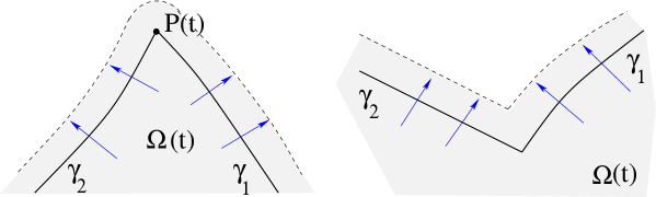
Figure 8: If no control is active, the set $\Omega(t)$ expands with speed $|\beta_{0}|$ in all directions. Hence outward corners instantly disappear (left), but inward corners persist (right).

Remark 7.1

If the control is not active along any of the two arcs $\gamma_{1},\gamma_{2}$, then the set $\Omega(t)$ expands with speed $|\beta_{0}|$ all along the boundary, in a neighborhood of $P(t)$. This implies that $\Omega(t)$ satisfies an interior ball condition, hence it can only have inward corners, as shown in Fig. 8.

Theorem 7.1

Let $E$ satisfy (A1), with (1.6) replaced by (7.1), and let $\phi:I\!\!R_{+}\mapsto I\!\!R_{+}$ be a ${\cal C}^{1}$ function which satisfies (A2). Assume that $t\mapsto\Omega(t)$ provides an optimal solution to (OP).

In the setting described at (A4), if along at least one of the two arcs $\gamma_{1},\gamma_{2}$ the control is active (i.e., if $\beta>\beta_{0}$ along the arc), then the two arcs must be tangent at $P(t)$.

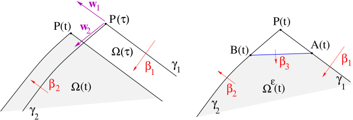
Figure 9: The case of outward corner. Left: the shaded region is the set $\Omega(t)$, for $t\in[\tau,\tau+\delta]$. Right: the set $\Omega^{\varepsilon}$ is obtained from $\Omega(t)$ by removing the triangular region $\widehat{APB}$.

Proof. 1. Assume that the two arcs $\gamma_{1},\gamma_{2}$ are not tangent, forming an angle $\theta(t)\neq\pi$ for $|\tau-t|<\delta$. We will then construct a perturbed multifunction $t\mapsto\Omega^{\varepsilon}(t)$ with a smaller cost. Given $0<\varepsilon<\!<\delta$, for $t\in[\tau-\varepsilon,\tau+\delta+\varepsilon]$ consider the points

$$A(t)~{}=~{}\left\{\begin{array}[]{cl}\gamma_{1}\bigl{(}t,\,\tau-t-\varepsilon\bigr{)}&\hbox{if}~{}~{}t\in[\tau-\varepsilon,\,\tau],\cr\gamma_{1}(t,-\varepsilon)&\hbox{if}~{}~{}t\in[\tau,\,\tau+\delta],\cr\gamma_{1}\bigl{(}t,\,t-\tau-\delta-\varepsilon)\bigr{)}&\hbox{if}~{}~{}t\in[\tau+\delta,\,\tau+\delta+\varepsilon],\end{array}\right.$$ (7.5)

$$B(t)~{}=~{}\left\{\begin{array}[]{cl}\gamma_{2}\bigl{(}t,\,t-\tau+\varepsilon\bigr{)}&\hbox{if}~{}~{}t\in[\tau-\varepsilon,\,\tau],\cr\gamma_{2}(t,\varepsilon)&\hbox{if}~{}~{}t\in[\tau,\,\tau+\delta],\cr\gamma_{2}\bigl{(}t,\,\tau+\delta+\varepsilon-t\bigr{)}&\hbox{if}~{}~{}t\in[\tau+\delta,\,\tau+\delta+\varepsilon].\end{array}\right.$$ (7.6)

Observe that $A(t)=B(t)=P(t)$ for $t=\tau-\varepsilon$ and for $t=\tau+\delta+\varepsilon$. We now construct a family of perturbed sets $\Omega^{\varepsilon}(t)$ by the following rules.

• For $t\notin[\tau-\varepsilon,\tau+\delta+\varepsilon]$, one has $\Omega^{\varepsilon}(t)~{}=~{}\Omega(t)$.

• If ${\bf w}_{1}\times{\bf w}_{2}>0$ (an outward corner), then for $t\in[\tau-\varepsilon,\tau+\delta+\varepsilon]$ the set $\Omega^{\varepsilon}(t)$ is obtained from $\Omega(t)$ by removing the triangular region with vertices $A(t),P(t),B(t)$, as shown in Fig. 9.

• If ${\bf w}_{1}\times{\bf w}_{2}<0$ (an inward corner), then for $t\in[\tau-\varepsilon,\tau+\delta+\varepsilon]$ the set $\Omega^{\varepsilon}(t)$ is obtained from $\Omega(t)$ by adding the triangular region with vertices $A(t),P(t),B(t)$, as shown in Fig. 10.

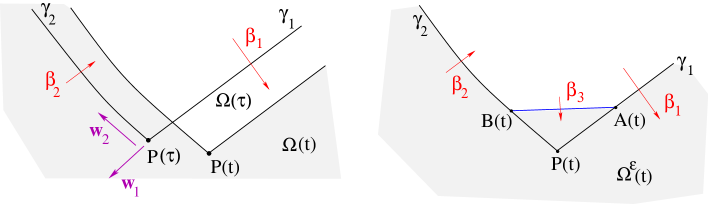
Figure 10: The case of an inward corner, with ${\bf w}_{1}\times{\bf w}_{2}<0$. Left: the shaded region is the set $\Omega(t)$, for $t\in[\tau,\tau+\delta]$. Right: the set $\Omega^{\varepsilon}$ is obtained from $\Omega(t)$ by adding the triangular region $\widehat{APB}$.

2. To estimate the change in the cost of the new strategy $\Omega^{\varepsilon}$, the crucial step is to determine the inward normal speed $\beta_{3}$ along the segment $\overline{A(t)B(t)}$. Referring to Fig. 11 consider a triangle with vertices

$$P(t),\qquad A(t)\,=\,P(t)-{\bf w}_{1},\qquad B(t)\,=\,P(t)+{\bf w}_{2}\,.$$

Call $\beta_{1},\beta_{2},\beta_{3}$ respectively the normal speeds of the three sides $AP$, $BP$, and $AB$. Knowing the velocity $\dot{P}=dP/dt$, these are computed by

$$\beta_{1}~{}=~{}\big{\langle}\dot{P},{\bf w}_{1}^{\perp}\big{\rangle},\qquad\beta_{2}~{}=~{}\big{\langle}\dot{P},{\bf w}_{2}^{\perp}\big{\rangle},\qquad\beta_{3}~{}=~{}\left\langle\dot{P},{({\bf w}_{1}+{\bf w}_{2})^{\perp}\over|{\bf w}_{1}+{\bf w}_{2}|}\right\rangle~{}=~{}{\beta_{1}+\beta_{2}\over|{\bf w}_{1}+{\bf w}_{2}|}.$$ (7.7)

Neglecting higher order terms, during the time interval $[\tau,\tau+\delta]$ the change in the total effort is thus computed as

$$\begin{array}[]{rl}{\cal E}^{\varepsilon}(t)-{\cal E}(t)&=~{}\varepsilon\Big{(}|{\bf w}_{1}+{\bf w}_{2}|\,E(\beta_{3})-E(\beta_{1})-E(\beta_{2})+{\cal O}(1)\cdot(\delta+\varepsilon)\Big{)}+o(\varepsilon)\\[8.53581pt] &=\displaystyle~{}\varepsilon\left(|{\bf w}_{1}+{\bf w}_{2}|\,E\left({\beta_{1}+\beta_{2}\over|{\bf w}_{1}+{\bf w}_{2}|}\right)-E(\beta_{1})-E(\beta_{2})\right)+{\cal O}(1)\cdot\delta\varepsilon+o(\varepsilon).\end{array}$$ (7.8)

We claim that, for $\varepsilon,\delta$ sufficiently small, the right hand side of (7.8) is strictly negative. Indeed, set

$$\overline{\beta}~{}\doteq~{}{\beta_{1}+\beta_{2}\over 2}~{}>~{}\beta_{0}\,\qquad\qquad\lambda~{}\doteq~{}{2\over|{\bf w}_{1}+{\bf w}_{2}|}~{}>~{}1\,.$$

Notice that the first inequality follows from the assumption that at least one of the normal speeds $\beta_{1},\beta_{2}$ is strictly larger than $\beta_{0}$. The second inequality is trivially true because ${\bf w}_{1},{\bf w}_{2}$ are non-parallel unit vectors. By the strict inequality (7.2) and the convexity of $E$ it now follows

$$\begin{array}[]{l}\displaystyle{1\over 2}\left[{|{\bf w}_{1}+{\bf w}_{2}|}\,E\left({\beta_{1}+\beta_{2}\over|{\bf w}_{1}+{\bf w}_{2}|}\right)-E(\beta_{1})-E(\beta_{2})\right]=~{}{1\over\lambda}E\left(\lambda\cdot{\beta_{1}+\beta_{2}\over 2}\right)-{E(\beta_{1})+E(\beta_{2})\over 2}\\[11.38109pt] \qquad<~{}\displaystyle E\left({\beta_{1}+\beta_{2}\over 2}\right)-{E(\beta_{1})+E(\beta_{2})\over 2}~{}\leq~{}0.\end{array}$$ (7.9)

By choosing $0<\varepsilon<\!<\delta$ sufficiently small, our claim is proved.

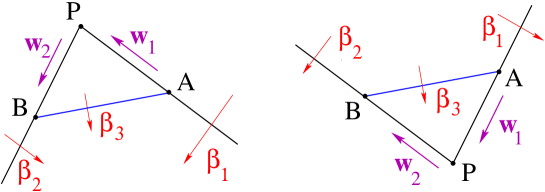
Figure 11: Computing the normal speed $\beta_{3}$ of the side $AB$, as in (7.7).

3. We now compare the cost of the two strategies $\Omega^{\varepsilon}(\cdot)$ and $\Omega(\cdot)$, for $0<\varepsilon<\!<\delta$ sufficiently small. For sake of definiteness, we consider an outward corner, so that ${\bf w}_{1}\times{\bf w}_{2}>0$. The case of an inward corner is entirely similar.

• Since $\Omega^{\varepsilon}(T)=\Omega(T)$, there is no difference in the terminal cost.

• For every $t\in[\tau-\varepsilon,\tau+\delta+\varepsilon]$ the difference in the area is bounded by

  $$\Big{|}m_{2}\bigl{(}\Omega^{\varepsilon}(t)\bigr{)}-m_{2}\bigl{(}\Omega(t)\bigr{)}\Big{|}~{}=~{}{\cal O}(1)\cdot\varepsilon^{2}.$$

  Integrating in time, this yields

  $$c_{1}\int_{0}^{T}m_{2}\bigl{(}\Omega^{\varepsilon}(t)\bigr{)}\,dt-c_{1}\int_{0}^{T}m_{2}\bigl{(}\Omega(t)\bigr{)}\,dt~{}=~{}{\cal O}(1)\cdot\varepsilon^{2}(\delta+2\varepsilon).$$ (7.10)

• At every time $t\in[\tau-\varepsilon,\,\tau+\delta+\varepsilon]$, the difference in the total effort is estimated by an integral of the effort over the segment with endpoints $A(t)$, $B(t)$. Namely

  $${\cal E}^{\varepsilon}(t)-{\cal E}(t)~{}\leq~{}\int_{\overline{A(t)\,B(t)}}E\bigl{(}\beta^{\varepsilon}(t,x)\bigr{)}\,d\sigma~{}=~{}{\cal O}(1)\cdot|B(t)-A(t)|~{}=~{}{\cal O}(1)\cdot\varepsilon.$$

  Since we are assuming the differentiability of the cost function $\phi$, this implies

  $$\left(\int_{\tau-\varepsilon}^{\tau}+\int_{\tau+\delta}^{\tau+\delta+\varepsilon}\right)\Big{[}\phi\bigl{(}{\cal E}^{\varepsilon}(t)\bigr{)}-\phi\bigl{(}{\cal E}(t)\bigr{)}\Big{]}\,dt~{}=~{}{\cal O}(1)\cdot\varepsilon^{2}.$$ (7.11)

• Finally, by the inequalities at (7.8)-(7.9), for $t\in[\tau,\tau+\delta]$, the difference in the total effort is bounded by

  $${\cal E}^{\varepsilon}(t)-{\cal E}(t)~{}\leq~{}-\varepsilon\kappa_{0}+o(\varepsilon),$$

  for some constant $\kappa_{0}>0$ and all $\delta,\varepsilon>0$ sufficiently small. Therefore, we can write

  $$\begin{array}[]{l}\displaystyle\int_{\tau}^{\tau+\delta}\Big{[}\phi\bigl{(}{\cal E}^{\varepsilon}(t)\bigr{)}-\phi\bigl{(}{\cal E}(t)\bigr{)}\Big{]}\,dt~{}\leq~{}\int_{\tau}^{\tau+\delta}{1\over 2}\phi^{\prime}\bigl{(}{\cal E}(t)\bigr{)}\cdot\bigl{[}{\cal E}^{\varepsilon}(t)-{\cal E}(t)\bigr{]}\,dt\\[11.38109pt] \displaystyle\qquad\qquad\leq~{}-\int_{\tau}^{\tau+\delta}{\kappa_{0}\over 4}\phi^{\prime}\bigl{(}{\cal E}(t)\bigr{)}~{}\leq~{}-\kappa_{1}\varepsilon\delta\,,\end{array}$$ (7.12)

  for some constant $\kappa_{1}>0$.

Combining the estimates (7.10), (7.11) and (7.12), the difference in the total cost is estimated as

$$J(\Omega^{\varepsilon})-J(\Omega)~{}\leq~{}-\kappa_{1}\varepsilon\delta+{\cal O}(1)\cdot\varepsilon^{2}~{}<~{}0,$$

showing that the original strategy was not optimal.MM     

8 Optimal motions determined by the necessary conditions

In this last section we study the set motions $t\mapsto\Omega(t)$ that satisfy the necessary conditions derived earlier. We focus on the basic case where

$$E(\beta)~{}=~{}\max\,\{0,\,1+\beta\}.$$ (8.1)

In connection with the optimality condition

$$\lambda(t)E\big{(}\beta(t,\xi)\bigr{)}-Y(t,\xi)\beta(t,\xi)~{}=~{}\min_{\beta\geq-1}~{}\Big{\{}\lambda(t)E(\beta)-Y(t,\xi)\beta\Big{\}},$$ (8.2)

three cases need to be considered.

CASE 1: $\lambda(t)-Y(t,\xi)>0$. In this case $\beta(t,\xi)=-1$. In other words, no effort is made at the point $x(t,\xi)$. Hence the boundary point $x(t,\xi)$ moves in the direction of the outer normal with unit speed.

CASE 2: $\lambda(t)-Y(t,\xi)=0$. In this case, any inward normal speed $\beta(t,\xi)\geq-1$ is compatible with (5.7).

CASE 3: $\lambda(t)-Y(t,\xi)<0$. This can never happen, because the minimality condition cannot be satisfied. Formally, (8.2) would imply that the optimal control is $\beta(t,\xi)=+\infty$.

Similarly to the case of singular controls, often encountered in geometric control theory [1, 5, 17], in Case 2 the pointwise values of $\beta(t,\xi)$ are determined not by the minimum principle (8.2), but by the requirement that the function $\xi\mapsto Y(t,\xi)=\lambda(t)$ is independent of $\xi$ on the region where the control is active. In other words, to determine the optimal normal speed $\beta=\beta(t,\xi)$ we need to use (5.4), and impose that the right hand side is constant w.r.t. $\xi$, over the portion of the boundary where the control is active. When the effort $E$ takes the simple form (8.1), the backward Cauchy problem (5.4)-(5.5) reduces to

$$Y_{t}(t,\xi)~{}=~{}\omega(t,\xi)Y(t,\xi)-c_{1}\,,\qquad\qquad Y(T,\xi)=c_{2}\,.$$ (8.3)

In order for $Y(t,\xi)=Y^{*}(t)$ to be a function of time alone, this implies the constant curvature condition:

• At any time $t\in[0,T]$ the curvature $\omega(t,\cdot)$ must be constant along the portion of the boundary where the control is active.

When the cost function $\phi$ is smooth, this constant value $\lambda(t)$ is determined by the scalar equation (5.6). On the other hand, when $\phi$ is the function in (1.9), $\lambda(t)$ can be determined by the global constraint

$$\int_{S}E(\beta(t,\xi))\,\bigl{|}x_{\xi}(t,\xi)\bigr{|}\,d\xi~{}=~{}M.$$ (8.4)

By the necessary conditions, the control is active at points $x(t,\xi)$ where the dual variable $Y(t,\xi)$ has the largest values. These are the points where it is most advantageous to shrink the set $\Omega(t)$. By (8.3), the characteristics $t\mapsto x(t,\xi)$ where the dual function $Y$ grows faster (going backwards in time) are those where the curvature is maximum, and the control is active. This leads to the following

Conjecture 8.1

At every time $t\in[0,T]$, the optimal control is active precisely along the portion of the boundary where the curvature is maximum.

The validity of this conjecture will be a topic for future investigation. Here we conclude with a simple example, where a motion satisfying the necessary conditions can be computed explicitly.

Example 8.1

Assume that the initial set $\Omega_{0}$ is a square with sides of length $a$, and let the cost functions $E,\phi$ be as in (1.9). Assuming that the control is applied along the portion of the boundary with maximum curvature, we describe here the evolution of the set $\Omega(t)$. As usual, we denote by $B(x,r)$ the open ball centered at $x$ with radius $r$, and by $B(\Omega_{0},\rho)$ the neighborhood of radius $\rho$ around the set $\Omega_{0}$. For $t,r>0$, consider the set

$$V(\Omega_{0},t,r)~{}\doteq~{}\bigcup\Big{\{}B(x,r)\,;~{}~{}B(x,r)\subseteq B(\Omega_{0},t)\Big{\}}.$$ (8.5)

This is the union of all balls of radius $r$ which are entirely contained inside $B(\Omega_{0},\rho)$.

  

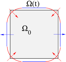
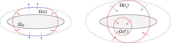
Figure 12: Left: the moving set $\Omega(t)$ in Example 8.1, where $\Omega_{0}$ is a square. Center and right: the moving set $\Omega(t)$, in the case where $\Omega_{0}$ is an ellipse and the control always acts on the portion of the boundary with maximum curvature.

In this case (see Fig. 12, left), the set $V(\Omega_{0},t,r)$ is obtained starting with a square of sides $a+2t$, and cutting out the regions near the four corners. The boundary of this set thus consists of four segments, and four arcs of circumferences of radius $r$. The perimeter and the area of the set $V(\Omega_{0},t,r)$ are computed as

$$\left\{\begin{array}[]{rl}P(t,r)&=~{}4(a+2t)-(8-2\pi)r,\\[2.84526pt] A(t,r)&=~{}(a+2t)^{2}-(4-\pi)r^{2}.\end{array}\right.$$ (8.6)

To derive an ODE for the function $r=r(t)$, we use the basic relation (1.10) and obtain

$${d\over dt}A\bigl{(}\bigl{(}t,r(t)\bigr{)}-P\bigl{(}t,r(t)\bigr{)}+M~{}=~{}-2(4-\pi)r\dot{r}(t)-(8-2\pi)r+M~{}=~{}0.$$ (8.7)

Solving the Cauchy problem

$${(8-2\pi)r\over M-(8-2\pi)r}\dot{r}~{}=~{}1\,,\qquad\qquad r(0)\,=\,0,$$ (8.8)

we determine $r(t)$ by the implicit equation

$$\lambda\,r(t)~{}=~{}1-e^{-\lambda\bigl{(}t+r(t)\bigr{)}}\,,\qquad\qquad\lambda~{}\doteq~{}{8-2\pi\over M}.$$ (8.9)

Notice that the function $t\mapsto r(t)$ depends on $M$, but not on $a$.

Next, the time $t_{1}$ when four arcs of circumferences join together is determined by the identity

$$a+2t_{1}~{}=~{}2r(t_{1}).$$

This yields the implicit equation

$$\lambda\left({a\over 2}+t_{1}\right)~{}=~{}1-\exp\left\{-\lambda\Big{(}2t_{1}+{a\over 2}\Big{)}\right\}.$$ (8.10)

Notice that (8.10) may not have a solution, if $M$ is too small. To check if a solution exists set

$$f(t)~{}\doteq~{}1-\exp\left\{-\lambda\Big{(}2t+{a\over 2}\Big{)}\right\},$$

and call

$$\tau~{}=~{}{1\over 2\lambda}\left(\ln 2-{a\lambda\over 2}\right)$$

the unique point where $f^{\prime}(\tau)=\lambda$. Then a solution to (8.10) exists if and only if

$$\lambda\left({a\over 2}+\tau\right)~{}\leq~{}1-\exp\left\{-\lambda\Big{(}2\tau+{a\over 2}\Big{)}\right\}.$$ (8.11)

We observe that a solution certainly exists if $4a<M$. In this case, the perimeter remains strictly smaller than $M$ at all times, and the set can be shrunk to the empty set in finite time. Finally, assuming that $t_{1}$ is well defined, for $t>t_{1}$ the optimal set $\Omega(t)$ is a disc whose radius satisfies

$${d\over dt}\bigl{(}\pi r^{2}(t)\bigr{)}~{}=~{}2\pi r(t)-M.$$

References

[1] A. Agrachev and M. Sigalotti,
On the local structure of optimal trajectories in .
SIAM J. Control Optim.42 (2003), 513–531.
[2] L. Ambrosio, N. Fusco, and D. Pallara,
Functions of Bounded Variation and Free Discontinuity Problems.
Clarendon Press, Oxford, 2000.
[3] S. Anita, V. Capasso, and G. Dimitriu,
Regional control for a spatially structured malaria model.
Math. Meth. Appl. Sci.42 (2019), 2909–2933.
[4] S. Anita, V. Capasso, and A. M. Mosneagu,
Global eradication for spatially structured populations by regional control.
Discr. Cont. Dyn. Syst., Series B, 24 (2019), 2511–2533.
[5]
U. Boscain and B. Piccoli
Optimal Syntheses for Control Systems on 2-D Manifolds. Springer-Verlag, Berlin, 2004.
[6] A. Bressan, Differential inclusions and the control of forest fires,
J. Differential Equations (special volume in honor of
A. Cellina and J. Yorke), 243 (2007), 179–207.
[7] A. Bressan, Dynamic blocking problems for a model of fire propagation.
In Advances in Applied Mathematics, Modeling,
and Computational Science, pp. 11–40.
R. Melnik and I. Kotsireas editors.
Fields Institute Communications, Springer, New York, 2013.
[8]
A. Bressan, M. T. Chiri, and N. Salehi, On the optimal control of propagation fronts,
submitted. Available on arXiv:2108.09321v1, 2021.
[9]
A. Bressan, M. Mazzola, and K. T. Nguyen,
Approximation of sweeping processes and controllability
for a set valued evolution, SIAM J. Control Optim.57 (2019), 2487–2514.
[10]
A. Bressan and B. Piccoli, Introduction to the Mathematical
Theory of Control, AIMS Series in Applied Mathematics, Springfield
Mo. 2007.
[11]
A. Bressan and D. Zhang, Control problems for a class of set valued evolutions,
Set-Valued Var. Anal.20 (2012), 581–601.
[12]
L. Cesari,
Optimization Theory and Applications,
Springer-Verlag, 1983.
[13]
R. M. Colombo and N. Pogodaev, On the control of moving sets: Positive and negative confinement results, SIAM J. Control Optim.51 (2013), 380–401.
[14]
R. M. Colombo, T. Lorenz and N. Pogodaev,
On the modeling of moving populations through set evolution equations.
Discrete Contin. Dyn. Syst.35 (2015), 73–98.
[15]
W.H. Fleming and R.W. Rishel,
Deterministic and Stochastic Optimal Control,
Springer-Verlag, New York, 1975.
[16] F. Maggi, Sets of Finite Perimeter and Geometric Variational Problems. Cambridge University Press, 2012.
[17]
H. J. Sussmann, The structure of time-optimal trajectories for single-input systems in the plane: The
nonsingular case, SIAM J. Control Optim.25 (1987), 433–465.