Local Spanners Revisited

Abstract

For a set of points $P\subseteq\mathbb{R}^{2}$, and a family of regions $\mathcal{F}$, a local $t$-spanner of $P$, is a sparse graph $G$ over $P$, such that, for any region $\mathcalb{r}\in\mathcal{F}$, the subgraph restricted to $\mathcalb{r}$, denoted by $G\cap{\mathcalb{r}}=G_{P\cap\mathcalb{r}}$, is a $t$-spanner for all the points of $\mathcalb{r}\cap P$.

We present algorithms for the construction of local spanners with respect to several families of regions, such as homothets of a convex region. Unfortunately, the number of edges in the resulting graph depends logarithmically on the spread of the input point set. We prove that this dependency can not be removed, thus settling an open problem raised by Abam and Borouny. We also show improved constructions (with no dependency on the spread) of local spanners for fat triangles, and regular $k$-gons. In particular, this improves over the known construction for axis parallel squares.

We also study a somewhat weaker notion of local spanner where one allows to shrink the region a “bit”. Any spanner is a weak local spanner if the shrinking is proportional to the diameter. Surprisingly, we show a near linear size construction of a weak spanner for axis-parallel rectangles, where the shrinkage is multiplicative.

1 Introduction

For a set $P$ of points in $\mathbb{R}^{d}$, the Euclidean graph $\mathcal{K}_{P}=\bigl{(}P,\binom{P}{2}\bigr{)}$ of $P$ is an undirected graph. Here, an edge $pq\in E$ is associated with the segment $pq$, and its weight is the (Euclidean) length of the segment. Let $G=(P,E)$ and $I=(P,E^{\prime})$ be two graphs over the same set of vertices (usually $I$ is a subgraph of $G$). Consider two vertices $p,q\in P$, and parameter $t\geq 1$. A path $\pi$ between $p$ and $q$ in $I$, is a $t$-path, if the length of $\pi$ in $I$ is at most $t\cdot\mathsf{d}_{G}\left({p,q}\right)$, where $\mathsf{d}_{G}\left({p,q}\right)$ is the length of the shortest path between $p$ and $q$ in $G$. The graph $I$ is a $t$-spanner of $G$ if there is a $t$-path in $I$, for any $p,q\in P$. Thus, for a set of points $P\subseteq\mathbb{R}^{d}$, a graph $G$ over $P$ is a $t$-spanner if it is a $t$-spanner of the euclidean graph $\mathcal{K}_{P}$. There is a lot of work on building geometric spanners, see [NS07] and references there in.

Fault-tolerant spanners

An $\mathcal{F}$-fault-tolerant spanner for $P\subseteq\mathbb{R}^{d}$, is a graph $G=(P,E)$, such that for any region $\mathcalb{r}$ (i.e., the “attack”), the graph $G-\mathcalb{r}$ is a $t$-spanner of $\mathcal{K}_{P}-\mathcalb{r}$ (See Definition 2.1 for a formal definition of this notation). Here $G-\mathcalb{r}$ denotes the graph after one deletes from $G$ all the vertices in $P\cap\mathcalb{r}$, and all the edges in $G$ that their corresponding segments intersect $\mathcalb{r}$. Surprisingly, as shown by Abam et al. [ABFG09], such fault-tolerant spanners can be constructed where the attack region is any convex set. Furthermore, these spanners have a near linear number of edges.

Fault-tolerant spanners were first studied with vertex and edge faults, meaning that some arbitrary set of maximum size $k$ of vertices and edges has failed. Levcopoulos et al. [LNS02] showed the existence of $k$-vertex/edges fault tolerant spanners for a set of points $P$ in some metric space. Their spanner had $\mathcal{O}(kn\log n)$ edges, and weight, i.e. sum of edge weights, bounded by $f(k)\cdot wt(MST(P))$ for some function $f$. Lukovszki [Luk99] later achieved a similar construction, improving the number of edges to $\mathcal{O}(kn)$, and was able to prove that the result is asymptotically tight.

Local spanners

Recently, Abam and Borouny [AB21] introduced the notion of local spanners. For a family of regions $\mathcal{F}$, a graph $G=(P,E)$ is a local $t$-spanner for $\mathcal{F}$, if for any $\mathcalb{r}\in\mathcal{F}$, the subgraph of $G$ induced on $P\cap\mathcalb{r}$ is a $t$-spanner. Specifically, this induced subgraph $G\cap{\mathcalb{r}}$ contains a $t$-path between any $p,q\in P\cap\mathcalb{r}$ (note that we keep an edge in the subgraph only if both its endpoints are in $\mathcalb{r}$, see Definition 2.1).

Abam and Borouny [AB21] showed how to construct such spanners for axis-parallel squares and vertical slabs. In this work, we are further extend their results. They also showed how to construct such spanners for disks if one is allowed to add Steiner points. Abam and Borouny left the question of how to construct local spanners for disks as an open problem.

To appreciate the difficulty in constructing local spanners, observe that unlike regular spanners, the construction has to take into account many different scenarios as far as which points are available to be used in the spanner. As a concrete example, a local spanner for axis-parallel rectangle requires quadratic number of edges, see Figure 1.1.

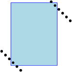
Figure 1.1: For any point in the top diagonal and bottom diagonal, there is a fat axis parallel rectangle that contains only these two points. Thus, a local spanner requires quadratic size in this case.

Namely, regular spanners can rely on using midpoints in their path under the assurance that they are always there. For local spanners this is significantly harder as natural midpoints might “disappear”. Intuitively, a local spanner construction needs to use midpoints that are guaranteed to be present judging only from the source and destination points of the path.

A good jump is hard to find

Most constructions for spanners can be viewed as searching for a way to build a path from the source to the destination by finding a “good” jump, either by finding a way to move locally from the source to a nearby point in the right direction, as done in the $\theta$-graph construction, or alternatively, by finding an edge in the spanner from the neighborhood of the source to the neighborhood of the destination, as done in the spanner constructions using well-separated pairs decomposition (WSPD). Usually, one argues inductively that the spanner must have (sufficiently short) paths from the source to the start of the jump, and from the end of the jump to the destination, and then, combining these implies that the resulting new path is short. These ideas guide our constructions as well. However, the availability of specific edges depends on the query region, making the search for a good jump significantly more challenging. The constructions have to guarantee that there are many edges available, and that at least one of them is useful as a jump regardless of the chosen region.

Region	# edges	Paper	New # edges	Location in paper
Local $(1+\varepsilon)$-spanners.
Halfplanes	$\mathcal{O}(\varepsilon^{-2}n\log n)\bigr{.}$	[ABFG09]
Axis-parallel squares	$\mathcal{O}_{\varepsilon}(n\log^{6}n)\Bigr{.}$	[AB21]	$\mathcal{O}\left({\varepsilon^{-3}n\log n}\right)$	Remark 3.20
Vertical slabs	$\mathcal{O}(\varepsilon^{-2}n\log n)\Bigr{.}$	[AB21]
Disks+Steiner points	$\mathcal{O}_{\varepsilon}(n)\Bigr{.}$	[AB21]
Disks			$\mathcal{O}\left({\varepsilon^{-2}n\log\Phi}\right)\Bigr{.}$	Theorem 3.6
			$\Omega(n\log\Phi)\Bigr{.}$	Lemma 3.10
Homothets convex shape			$\mathcal{O}\left({\varepsilon^{-2}n\log\Phi}\right)\Bigr{.}$	Theorem 3.6
Homothets $\alpha$-fat triangles			$\mathcal{O}\left({(\alpha\varepsilon)^{-1}n}\right)\Bigr{.}$	Theorem 3.16
Homothets triangles			$\Omega\left({n\log\Phi}\right)\Bigr{.}$	Lemma 3.11
$\delta$-weak local $(1+\varepsilon)$-spanners.
Bounded convex shape			$\mathcal{O}\bigl{(}(\varepsilon^{-1}+\delta^{-2})n\bigr{)}\Bigr{.}$	Lemma 2.12
$(1-\delta)$-local $(1+\varepsilon)$-spanners.
Axis-parallel rectangles			$\mathcal{O}\bigl{(}(\varepsilon^{-2}+\delta^{-2})n\log^{2}n\bigr{)}\Bigr{.}$	Theorem 4.6

Table 1.1: Known and new results. The notation $\mathcal{O}_{\varepsilon}$ hides polynomial dependency on $\varepsilon$ which is not specified in the original work.

Our results

Our results are summarized in Table 1.1.

Almost local spanners

We start by showing that regular geometric spanners are local spanners if one is required provide the spanner guarantee only to shrunken regions. Namely, if $G$ is a $(1+\varepsilon)$-spanner of $P$, then for any convex region $\mathcal{C}$, the graph $G\cap{\mathcal{C}}$ is a spanner for $\mathcal{C}^{\prime}\cap P$, where $\mathcal{C}^{\prime}$ is the set of all points in $\mathcal{C}$ that are in distance at least $\varepsilon\cdot\mathrm{diam}\left({\mathcal{C}}\right)$ from its boundary.

Homothets

A homothet of a convex region $\mathcal{C}$, is a translated and scaled copy of $\mathcal{C}$. In Section 3 we present a construction of spanners, which surprisingly, is not only fault-tolerant for all convex regions, but is also a local spanner for homothets of a prespecified convex region. This in particular works for disks, and resolves the aforementioned open problem of Abam and Borouny [AB21]. Our construction is somewhat similar to the original construction of Abam et al. [ABFG09]. For a parameter $\varepsilon>0$ the construction of a $(1+\varepsilon)$-local spanner for homothets takes $\mathcal{O}\left({\varepsilon^{-2}n\log\Phi\log n}\right)$ time, and the resulted spanner is of size $\mathcal{O}\left({\varepsilon^{-2}n\log\Phi}\right)$, where $\Phi$ is the spread of the input point set $P$, and $n=|P|$. We also provide a lower bound showing that this logarithmic dependency on $\Phi$ cannot be avoided.

The dependency on the spread $\Phi$ in the above construction is somewhat disappointing. However. the lower bound constructions, provided in Section 3.3, show that this is unavoidable for disks or homothets of triangles.

Thus, the natural question is what are the cases where one can avoid the “curse of the spread” – that is, cases where one can construct local spanners of near-linear size independent of the spread of the input point set.

The basic building block: $\mathcal{C}$-Delaunay triangulation

A key ingredient in the above construction is the concept of Delaunay triangulations induced by homothets of a convex body. Intuitively, one replaces the unit disk (of the standard $L_{2}$-norm) by the provided convex region. It is well known [CD85] that such diagrams exist, have linear complexity in the plane, and can be computed quickly. In Section 3.1 we review these results, and restate the well-known property that the $\mathcal{C}$-Delaunay triangulation is connected when restricted to a homothet of $\mathcal{C}$. By computing these triangulations for carefully chosen subsets of the input point set, we get the results stated above.

Specifically, we use well-separated and semi-separated decompositions to compute these subsets.

Fat triangles

In Section 3.4 we give a construction of local spanners for the family $\mathcal{F}$ of homothets of a given triangle $\triangle$, and get a spanner of size $\mathcal{O}\left({(\alpha\varepsilon)^{-1}n}\right)$ in $\mathcal{O}\left({(\alpha\varepsilon)^{-1}n\log n}\right)$ time, where $\alpha$ is the smallest angle in $\triangle$. This construction is a careful adaptation of the $\theta$-graph spanner construction to the given triangle, and it is significantly more technically challenging than the original construction.

$k$-regular polygons

It seems natural that if one can handle fat triangles, then homothets of $k$-regular polygons should readily follow by a simple decomposition of the polygon into fat triangles. Maybe surprisingly, this is not the case – a critical configuration might involve two points that are on the interior of two non-adjacent edges of a homothet of the input polygon. We overcome this by first showing that sufficiently narrow trapezoids, provide us with a good jump somewhere inside the trapezoid, assuming one computes the Delaunay triangulation induced by the trapezoid, and that the source and destination lie on the two legs of the trapezoid. Next, we show that such a polygon can be covered by a small number of narrow trapezoids and fat triangles. By building appropriate graphs for each trapezoid/triangle in the collection, we get a spanner for homothets of the given $k$-regular polygon, with size that has no dependency on the spread. Of course, the size does depend on $k$. See Section 3.5 for details, and Theorem 3.19 for the precise result.

Quadrant separated pair decomposition (QSPD)

In Appendix 4.1, we describe a novel pair-decomposition. Specifically, the QSPD breaks the input point set $P$ into pairs, such that for any pair $\{X,Y\}$ we have the property that there is a translated axis system such that $X$ and $Y$ belong to two antipodal quadrants. In $d$ dimensions there is such a decomposition with $\mathcal{O}(n\log^{d-1}n)$ pairs, and total weight $\mathcal{O}(n\log^{d}n)$. A somewhat similar idea was used by Abam and Borouny [AB21] for the $d=1$ case. We believe this decomposition might be useful and is of independent interest.

Multiplicative weak local spanner for rectangles

In Appendix 4.2, we use QSPDs to construct a weak local spanner for axis parallel rectangles. Here, the constructed graph $G$ over $P$, has the property that for any axis-parallel rectangle ${R}$, the graph $G\cap{{R}}$ is a $(1+\varepsilon)$-spanner for all the points of $\bigl{(}(1-\varepsilon){R}\bigr{)}\cap P$, where $(1-\varepsilon){R}$ is the scaling of the rectangle by a factor of $1-\varepsilon$ around its center. Importantly, this works for narrow rectangles where this form of multiplicative shrinking is still meaningful (unlike the diameter based shrinking mentioned above). Contrast this with the lower bound (illustrated in Figure 1.1) of $\Omega(n^{2})$ on the size of local spanner if one does not shrink the rectangles. See Theorem 4.6 for details of the precise result.

See Table 1.1 for a summary of known results and comparisons to the results of this paper.

2 Preliminaries

Residual graphs

Definition 2.1.

Let $\mathcal{F}$ be a family of regions in the plane. For a fault region $\mathcalb{r}\in\mathcal{F}$ and a geometric graph $G$ on a point set $P$, let $G-\mathcalb{r}$ be the residual graph after removing from it all the points of $P$ in $\mathcalb{r}$ and all the edges that their corresponding segments intersect $\mathcalb{r}$. Similarly, let $G\cap{\mathcalb{r}}$ denote the graph restricted to $\mathcalb{r}$. Formally, let

$$G-\mathcalb{r}=\bigl{(}P\setminus\mathcalb{r},\left\{uv\in E\;\middle|\;uv\cap\mathrm{int}\left({\mathcalb{r}}\right)=\emptyset\right\}\bigr{)}\qquad\text{and}\qquad G\cap{\mathcalb{r}}=\bigl{(}P\cap{\mathcalb{r}},\left\{uv\in E\;\middle|\;uv\subseteq{\mathcalb{r}}\right\}\bigr{)}.$$

where $\mathrm{int}\left({\mathcalb{r}}\right)$ denotes the interior of $\mathcalb{r}$.

2.1 On various pair decompositions

For sets $X,Y$, let $X\otimes Y=\left\{\left\{{x,y}\right\}\;\middle|\;x\in X,\,y\in Y,x\neq y\right\}$ be the set of all the (unordered) pairs of points formed by the sets $X$ and $Y$.

Definition 2.2 (Pair decomposition).

For a point set $P$, a pair decomposition of $P$ is a set of pairs

$$\mathcal{W}=\left\{{\bigl{.}\left\{{X_{1},Y_{1}}\right\},\ldots,\left\{{X_{s},Y_{s}}\right\}}\right\},$$

such that (I) $X_{i},Y_{i}\subseteq P$for every $i$, (II) $X_{i}\cap Y_{i}=\emptyset$for every $i$, and (III) $\bigcup_{i=1}^{s}X_{i}\otimes Y_{i}=P\otimes P$. Its weight is $\omega\left({\mathcal{W}}\right)=\sum_{i=1}^{s}\left({\left|{X_{i}}\right|+\left|{Y_{i}}\right|}\right)$.

The closest pair distance of a set of points $P\subseteq\mathbb{R}^{d}$, is $\mathrm{c{}p}\left({P}\right)=\underset{p,q\in P,p\neq q}{\min}\left\|pq\right\|.$ The diameter of $P$ is $\mathrm{diam}\left({P}\right)=\underset{p,q\in P}{\max}\left\|pq\right\|.$ The spread of $P$ is $\Phi\left({P}\right)=\mathrm{diam}\left({P}\right)/\mathrm{c{}p}\left({P}\right)$, which is the ratio between the diameter and closest pair distance. While in general the weight of a WSPD (defined below) can be quadratic, if the spread is bounded, the weight is near linear. For $X,Y\subseteq\mathbb{R}^{d}$, let $\mathsf{d}\left({X,Y}\right)=\underset{p\in X,q\in Y}{\min}\left\|pq\right\|$ be the distance between the two sets.

Definition 2.3.

Two sets $X,Y\subseteq\mathbb{R}^{d}$ are

$$1/\varepsilon \text{if}\qquad\mathbf{max}\left({\mathrm{d{}i{}am}\left({X}\right),\mathrm{d{}i{}am}\left({Y}\right)}\right)\leq\varepsilon\cdot\mathsf{d}\left({X,Y}\right),$$-well-separated

and$$1/\varepsilon \text{if}\qquad\mathbf{min}\left({\mathrm{d{}i{}am}\left({X}\right),\mathrm{d{}i{}am}\left({Y}\right)}\right)\leq\varepsilon\cdot\mathsf{d}\left({X,Y}\right).$$-semi-separated

For a point set $P$, a well-separated pair decomposition (WSPD) of $P$ with parameter $1/\varepsilon$ is a pair decomposition of $P$ with a set of pairs $\mathcal{W}=\left\{{\bigl{.}\left\{{B_{1},C_{1}}\right\},\ldots,\left\{{B_{s},C_{s}}\right\}}\right\},$ such that for all $i$, the sets $B_{i}$ and $C_{i}$ are $(1/\varepsilon)$-separated. The notion of $1/\varepsilon$-SSPD (a.k.a semi-separated pairs decomposition) is defined analogously.

Lemma 2.4 ([AH12]).

Let $P$ be a set of $n$ points in $\mathbb{R}^{d}$, with spread $\Phi=\Phi\left({P}\right)$, and let $\varepsilon>0$ be a parameter. Then, one can compute a $(1/\varepsilon)$-WSPD $\mathcal{W}$ for $P$ of total weight $\omega\left({\mathcal{W}}\right)=\mathcal{O}(n\varepsilon^{-d}\log\Phi)$. Furthermore, any point of $P$ participates in at most $\mathcal{O}\left({\varepsilon^{-d}\log\Phi}\right)$ pairs.

Theorem 2.5 ([AH12, Har11]).

Let $P$ be a set of $n$ points in $\mathbb{R}^{d}$, and let $\varepsilon>0$ be a parameter. Then, one can compute a $(1/\varepsilon)$-SSPD for $P$ of total weight $\mathcal{O}\left({n\varepsilon^{-d}\log n}\right)$. The number of pairs in the SSPD is $\mathcal{O}\left({n\varepsilon^{-d}}\right)$, and the computation time is $\mathcal{O}\left({n\varepsilon^{-d}\log n}\right)$.

Lemma 2.6.

Given an $\alpha$-SSPD $\mathcal{W}$ of a set $P$ of $n$ points in $\mathbb{R}^{d}$ and a parameter $\beta\geq 2$, one can refine $\mathcal{W}$ into an $\alpha\beta$-SSPD $\mathcal{W}^{\prime}$, such that $|\mathcal{W}^{\prime}|=\mathcal{O}(|\mathcal{W}|/\beta^{d})$ and $\omega\left({\mathcal{W}^{\prime}}\right)=\mathcal{O}(\omega\left({\mathcal{W}}\right)/\beta^{d})$.

Proof:

The algorithm scans the pairs of $\mathcal{W}$. For each pair $\Xi=\{X,Y\}\in\mathcal{W}$, assume that $\mathrm{d{}i{}am}\left({X}\right)<\mathrm{d{}i{}am}\left({Y}\right)$. Let $\mathcalb{s}$ be the smallest axis-parallel cube containing $X$, and denote its sidelength by $r$. Let $r^{\prime}=r/\left\lceil{\sqrt{d}\beta}\right\rceil$. Partition $\mathcalb{s}$ into a grid of cubes of sidelength $r^{\prime}$, and let $T_{\Xi}$ be the resulting set of squares. The algorithm now add the set pairs

$$\left\{\{X\cap\mathcalb{t},Y\}\;\middle|\;\mathcalb{t}\in T_{\Xi}\right\}$$

to the output SSPD. Clearly, the resulting set is now $\alpha\beta$-semi separated, as we chopped the smaller part of each pair into $\beta$ smaller portions.  

Definition 2.7.

An $\varepsilon$-double-wedge is a region between two lines, where the angle between the two lines is at most $\varepsilon$.

Two point sets $X$ and $Y$ that each lie in their own cone of a shared $\varepsilon$-double-wedge are $\varepsilon$-angularly separated.

Lemma 2.8 (Proof in Appendix A).

Given a $(1/\varepsilon)$-SSPD $\mathcal{W}$ of $n$ points in the plane, one can refine $\mathcal{W}$ into a $(1/\varepsilon)$-SSPD $\mathcal{W}^{\prime}$, such that each pair $\Xi=\{X,Y\}\in\mathcal{W}^{\prime}$ is contained in a $\varepsilon$-double-wedge $\times_{\Xi}$, such that $X$ and $Y$ are contained in the two different faces of the double wedge $\times_{\Xi}$. We have that $|\mathcal{W}^{\prime}|=\mathcal{O}(|\mathcal{W}|/\varepsilon)$ and $\omega\left({\mathcal{W}^{\prime}}\right)=\mathcal{O}(\omega\left({\mathcal{W}}\right)/\varepsilon)$. The construction time is proportional to the weight of $\mathcal{W}^{\prime}$.

Corollary 2.9.

Let $P$ be a set of $n$ points in the plane, and let $\varepsilon>0$ be a parameter. Then, one can compute a $(1/\varepsilon)$-SSPD for $P$ such that every pair is $\varepsilon$-angularly separated. The total weight of the SSPD is $\mathcal{O}\left({n\varepsilon^{-3}\log n}\right)$, the number of pairs in the SSPD is $\mathcal{O}\left({n\varepsilon^{-3}}\right)$, and the computation time is $\mathcal{O}\left({n\varepsilon^{-3}\log n}\right)$.

2.2 Weak local spanners for fat convex regions

Definition 2.10.

Given a convex region $C$, let

$$C_{\boxminus\delta}=\left\{p\in C\;\middle|\;\mathsf{d}\left({p,\mathbb{R}^{2}\setminus C}\right)\geq\delta\cdot\mathrm{d{}i{}am}\left({C}\right)\right\}.$$

Formally, $C_{\boxminus\delta}$ is the Minkowski difference of $C$ with a disk of radius $\delta\cdot\mathrm{d{}i{}am}\left({C}\right)$.

Definition 2.11.

Consider a (bounded) set $C$ in the plane. Let $r_{\mathrm{in}}\left({C}\right)$ be the radius of the largest disk contained inside $C$. Similarly, $R_{\mathrm{out}}\left({C}\right)$ is the smallest radius of a disk containing $C$.

The aspect ratio of a region $C$ in the plane is $\mathsf{a{}r}\left({C}\right)=R_{\mathrm{out}}\left({C}\right)/r_{\mathrm{in}}\left({C}\right)$. Given a family $\mathcal{F}$ or regions in the plane, its aspect ratio is $\mathsf{a{}r}\left({\mathcal{F}}\right)=\max_{C\in\mathcal{F}}\mathsf{a{}r}\left({C}\right)$.

Note, that if a convex region $C$ has bounded aspect ratio, then $C_{\boxminus\delta}$ is similar to the result of scaling $C$ by a factor of $1-\mathcal{O}(\delta)$. On the other hand, if $C$ is long and skinny then this region is much smaller. Specifically, if $C$ has width smaller than $2\delta\cdot\mathrm{d{}i{}am}\left({C}\right)$, then $C_{\boxminus\delta}$ is empty.

Lemma 2.12.

Given a set $P$ of $n$ points in the plane, and parameters $\delta,\varepsilon\in(0,1)$. One can construct a graph $G$ over $P$, in $\mathcal{O}((\varepsilon^{-1}+\delta^{-2})n\log n)$ time, and with $\mathcal{O}\bigl{(}(\varepsilon^{-1}+\delta^{-2})n\bigr{)}$ edges, such that for any (bounded) convex $C$ in the plane, we have that for any two points $p,q\in P\cap C_{\boxminus\delta}$ the graph $C\cap{P}$ has $(1+\varepsilon)$-path between $p$ and $q$.

Proof:

Let $\vartheta=\min(\varepsilon,\delta^{2})$. Construct, in $\mathcal{O}(\vartheta^{-1}n\log n)$ time, a standard $(1+\vartheta)$-spanner $G$ for $P$ using $\mathcal{O}(\vartheta^{-1}n)$ edges [AMS99].

So, consider any body $C\in\mathcal{F}$, and any two vertices $p,q\in P\cap C^{\prime}$, where $C^{\prime}=C_{\boxminus\delta}$, Let $\ell=\left\|pq\right\|$, let $\pi$ be the shortest path between $p$ and $q$ in $G$, and let $\mathcal{E}$ be the locus of all points $u$, such that $\left\|pu\right\|+\left\|uq\right\|\leq(1+\vartheta)\ell$. The region $\mathcal{E}$ is an ellipse that contains $\pi$. The furthest point from the segment $pq$ in this ellipse is realized by the co-vertex of the ellipse. Formally, it is one of the two intersection points of the boundary of the ellipse with the line orthogonal to $pq$ that passes through the middle point $c$ of this segment, see Figure 2.1. Let $z$ be one of these points.

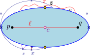
Figure 2.1: An illustration of the settings in the proof of Lemma 2.12 with $\mathcal{E}$ shown in blue.

We have that $\left\|pz\right\|=(1+\vartheta)\ell/2.$ Setting $h=\left\|zc\right\|$, we have that

$$h=\sqrt{\left\|pz\right\|^{2}-\left\|pc\right\|^{2}}=\frac{\ell}{2}\sqrt{(1+\vartheta)^{2}-1}=\frac{\sqrt{\vartheta(2+\vartheta)}}{2}\ell\leq\sqrt{\vartheta}\ell\leq\sqrt{\vartheta}\cdot\mathrm{d{}i{}am}\left({C}\right).$$

as $\ell\leq\mathrm{d{}i{}am}\left({C^{\prime}}\right)\leq\mathrm{d{}i{}am}\left({C}\right)$.

For any point $x\in C^{\prime}$, we have that $\mathsf{d}\left({x,\mathbb{R}^{2}\setminus C}\right)\geq\delta\cdot\mathrm{diam}\left({C}\right)$. As such, to ensure that $\pi\subseteq\mathcal{E}\subseteq C$, we need that $\delta\cdot\mathrm{diam}\left({C}\right)\geq h,$ which holds if $\delta\cdot\mathrm{diam}\left({C}\right)\geq\sqrt{\vartheta}\cdot\mathrm{d{}i{}am}\left({C}\right).$ This in turn holds if $\vartheta\leq\delta^{2}$. Namely, we have the desired properties if $\vartheta=\min(\varepsilon,\delta^{2})$.  

3 Local spanners of homothets of convex region

Let $\mathcal{C}$ be a bounded convex and closed region in the plane (e.g., a disk). A homothet of $\mathcal{C}$ is a scaled and translated copy of $\mathcal{C}$. A point set $P$ is in general position with respect to $\mathcal{C}$, if no four points of $P$ lie on the boundary of a homothet of $\mathcal{C}$, and no three points are colinear.

A graph $G=(P,E)$ is a $\mathcal{C}$-local $t$-spanner for $P$ if for any homothet $\mathcalb{r}$ of $\mathcal{C}$ we have that $G\cap{\mathcalb{r}}$ is a $t$-spanner of $\mathcal{K}_{P}\cap\mathcalb{r}$.

3.1 Delaunay triangulation for homothets

Definition 3.1 ([CD85]).

Given $\mathcal{C}$ as above, and a point set $P$ in general position with respect to $\mathcal{C}$, the $\mathcal{C}$-Delaunay triangulation of $P$, denoted by $\mathcal{D}_{\mathcal{C}}(P)$, is the graph formed by edges between any two points $p,q\in P$ such that there is a homothet of $\mathcal{C}$ that contains only $p$ and $q$ and no other point of $P$.

Theorem 3.2 ([CD85]).

For any convex shape $\mathcal{C}$ and a set of points $P$, $\mathcal{D}_{\mathcal{C}}(P)$ can be computed in $\mathcal{O}(n\log n)$ time. Furthermore, the triangulation $\mathcal{D}_{\mathcal{C}}(P)$ has $\mathcal{O}(n)$ edges, vertices, and faces.

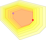
Figure 3.1: Shrinking of homothets so two points becomes on the boundary of the homothet.

Lemma 3.3.

Let $\mathcal{C}$ be a convex bounded body, and let $P$ be a set of points in general position with respect to $\mathcal{C}$. Then, if $C$ is a homothet of $\mathcal{C}$ that contains two points $p,q\in\mathcal{C}\cap P$, then there exists a homothet $C^{\prime}\subseteq C$ of $\mathcal{C}$ such that $p,q\in\partial C^{\prime}$.

Proof:

The idea is to apply a shrinking process of $C$, as illustrated in Figure 3.1. Consider the mapping $f_{\beta,v}:x\mapsto\beta(x-v)+v$. It is a scaling of the plane around $v$ by a factor of $\beta$. Let $\beta^{\prime}$ be the minimum value of $\beta$ such that $C_{1}=f_{\beta,p}(C)$ contains $q$ (i.e., we shrink $C$ around $p$ till $q$ becomes a boundary point). Next, shrink $C^{\prime}$ around $q$, till $p$ becomes a boundary point – formally, let $\beta^{\prime\prime}$ be the minimum value of $\beta$ such that $C^{\prime}=f_{\beta,q}(C_{1})$ contains $p$. Since $C^{\prime}\subseteq C_{1}\subseteq C$, and $p,q\in\partial C^{\prime}$, the claim follows.  

The following standard claim, usually stated for the standard Delaunay triangulations, also holds for homothets.

Claim 3.4.

Let $\mathcal{C}$ be a bounded close convex shape. Given a set of points $P\subseteq\mathbb{R}^{2}$ in general position with respect to $\mathcal{C}$, let $\mathcal{D}=\mathcal{D}_{\mathcal{C}}(P)$ be the $\mathcal{C}$-Delaunay triangulation of $P$. For any homothet $C$ of $\mathcal{C}$, we have that $\mathcal{D}\cap{C}$ is connected.

Proof:

We prove that for any homothet $C$ with two points $p,q\in P$ on its boundary, there is a path between $p$ and $q$ in $\mathcal{D}\cap{C}$, and Lemma 3.3 will immediately imply the general statement. The proof is by induction over the number $m$ of points of $P$ in the interior of $C$. If $m=0$ then $C$ contains no points of $P$ in its interior, and thus $pq$ is an edge of the Delaunay triangulation, as $C$ testifies.

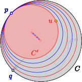
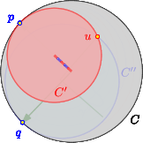
Figure 3.2: An illustration of the proof of Claim 3.4 in the case that $C$ is a disk.

Otherwise, let $u\in P$ be a point in the interior of $C$. From Lemma 3.3 we get that there exists a homothet $C^{\prime}$ of $C$ with $C^{\prime}\subseteq C$, such that $p$ and $u$ lie on the boundary of $C^{\prime}$ Thus, by induction, there is a path $\gamma^{\prime}$ between $p$ and $u$ in $\mathcal{D}\cap{C^{\prime}}\subseteq\mathcal{D}\cap{C}$. Similarly, there must be a homothet $C^{\prime\prime}$, that gives rise to a path $\gamma^{\prime\prime}$ between $u$ and $q$, and concatenating the two paths results in a path between $p$ and $q$ in $\mathcal{D}\cap{C}$.  

3.2 The generic construction

The input is a set $P$ of $n$ points in the plane (in general position) with spread $\Phi=\Phi\left({P}\right)$, and a parameter $\varepsilon\in(0,1)$. We have a convex body $\mathcal{C}$ that defines the “unit” ball. The task is to construct a local spanner for any homothet of $\mathcal{C}$.

The algorithm computes a $(1/\vartheta)$-WSPD $\mathcal{W}$ of $P$ using the algorithm of Lemma 2.4, where $\vartheta=\varepsilon/6$. For each pair $\Xi=\{X,Y\}\in\mathcal{W}$, the algorithm computes the $\mathcal{C}$-Delaunay triangulation $\mathcal{D}_{\Xi}=\mathcal{D}_{\mathcal{C}}(X\cup Y)$. The algorithm adds all the edges in $\mathcal{D}_{\Xi}\cap(X\otimes Y)$ to the computed graph $G$.

3.2.1 Analysis

Size

For each pair $\Xi=\{X,Y\}$ in the WSPD, its $\mathcal{C}$-Delaunay triangulation contains at most $\mathcal{O}(|X|+|Y|)$ edges. As such, the number of edges in the resulting graph is bounded by $\sum_{\{X,Y\}\in\mathcal{W}}O\bigl{(}|X|+|Y|\bigr{)}=\mathcal{O}\left({\omega\left({\mathcal{W}}\right)}\right)=\mathcal{O}\left({\frac{n\log\Phi}{{\vartheta}^{2}}}\right),$ by Lemma 2.4.

Construction time

The construction time is bounded by

$$\sum_{\{X,Y\}\in\mathcal{W}}O\bigl{(}(|X|+|Y|)\log(|X|+|Y|)\bigr{)}=\mathcal{O}\left({\omega\left({\mathcal{W}}\right)\log n}\right)=\mathcal{O}\left({\frac{n\log\Phi\log n}{{\vartheta}^{2}}}\right).$$

Lemma 3.5 (Local spanner property).

For $P,\mathcal{C},\varepsilon$ as above, let $G$ be the graph constructed above for the point set $P$. Then, for any homothet $C$ of $\mathcal{C}$ and any two points $x,y\in P\cap C$, we have that $G\cap{C}$ has a $(1+\varepsilon)$-path between $x$ and $y$. That is, $G$ is a $\mathcal{C}$-local $(1+\varepsilon)$-spanner.

Proof:

Fix a homothet $C$ of $\mathcal{C}$, and consider two points $p,q\in P\cap C$. The proof is by induction on the distance between $p$ and $q$ (or more precisely, the rank of their distance among the $\binom{n}{2}$ pairwise distances). Consider the pair $\Xi=\{X,Y\}$ such that $x\in X$ and $y\in Y$.

If $xy\in\mathcal{D}_{\Xi}$ then the claim holds, so assume this is not the case. By the connectivity of $\mathcal{D}_{\Xi}\cap C$, see Claim 3.4, there must be points $x^{\prime}\in X\cap C$, $y^{\prime}\in Y\cap C$, such that $x^{\prime}y^{\prime}\in E\left({\mathcal{D}_{\Xi}}\right)$. As such, by construction, we have that $x^{\prime}y^{\prime}\in E\left({G}\right)$. Furthermore, by the separation property, we have that

$$\max\left({\mathrm{d{}i{}am}\left({X}\right),\mathrm{d{}i{}am}\left({Y}\right)}\right)\leq\vartheta\,\mathsf{d}\left({X,Y}\right)\leq\vartheta\ell,$$

where $\ell=\left\|xy\right\|$. In particular, $\left\|x^{\prime}x\right\|\leq\vartheta\ell$ and $\left\|y^{\prime}y\right\|\leq\vartheta\ell$. As such, by induction, we have $\mathsf{d}_{G}\left({x,x^{\prime}}\right)\leq(1+\varepsilon)\left\|xx^{\prime}\right\|\leq(1+\varepsilon)\vartheta\ell$ and $\mathsf{d}_{G}\left({y,y^{\prime}}\right)\leq(1+\varepsilon)\left\|yy^{\prime}\right\|\leq(1+\varepsilon)\vartheta\ell$. Furthermore, $\left\|x^{\prime}y^{\prime}\right\|\leq(1+2\vartheta)\ell$. As $x^{\prime}y^{\prime}\in E\left({G}\right)$, we have

$$\mathsf{d}_{G}\left({x,y}\right) \leq\mathsf{d}_{G}\left({x,x^{\prime}}\right)+\left\|x^{\prime}y^{\prime}\right\|+\mathsf{d}_{G}\left({y^{\prime},y}\right)\leq(1+\varepsilon)\vartheta\ell+(1+2\vartheta)\ell+(1+\varepsilon)\vartheta\ell\leq\left({2\vartheta+1+2\vartheta+2\vartheta}\right)\ell$$

$$=\left({1+6\vartheta}\right)\ell\leq\left({1+\varepsilon}\right)\left\|xy\right\|,$$

if $\vartheta\leq\varepsilon/6$.  

The result

We thus get the following.

Theorem 3.6.

Let $\mathcal{C}$ be a bounded convex shape in the plane, let $P$ be a given set of $n$ points in the plane (in general position), and let $\varepsilon\in(0,1/2)$ be a parameter. The above algorithm constructs a $\mathcal{C}$-local $(1+\varepsilon)$-spanner $G$. The spanner has $\mathcal{O}\left({\varepsilon^{-2}n\log\Phi}\right)$ edges, and the construction time is $\mathcal{O}\left({\varepsilon^{-2}n\log\Phi\log n}\right)$. Formally, for any homothet $C$ of $\mathcal{C}$, and any two points $p,q\in P\cap C$, we have a $(1+\varepsilon)$-path in $G\cap{C}$.

3.2.2 Applications and comments

The following defines a “visibility” graph when we are restricted to a region $R$, where two points are visible if there is a witness homothet contained in $R$ having both points on its boundary.

Definition 3.7.

Let $\mathcal{C}$ be a bounded convex shape in the plane. Given a region $R$ in the plane and a point set $P$, consider two points $p,q\in P$. The edge $pq$ is safe in $R$ if there is a homothet $C$ of $\mathcal{C}$, such that $p,q\in C\subseteq R$. The safe graph for $P$ and $R$, denoted by $\mathcal{S}\left({P,R}\right)$, is the graph formed by all the safe edges in $P$ for $R$. Note, that this graph might have a quadratic number of edges in the worst case.

Observe that $\mathcal{S}\left({P,\mathbb{R}^{2}}\right)$ is a clique. Surprisingly, the spanner graph described above, when restricted to region $R$, is a spanner for $\mathcal{S}\left({P,R}\right)$.

Corollary 3.8.

Let $\mathcal{C}$ be a bounded convex body, $P$ be a set of $n$ points in the plane, $\varepsilon\in(0,1)$ be a parameter, and let $G$ be a $\mathcal{C}$-local $(1+\varepsilon)$-spanner of $P$.

Consider a region $R$ in the plane, and the associated graph $H=\mathcal{S}\left({P,R}\right)$, we have that $G\cap{R}$ is a $(1+\varepsilon)$-spanner for $H$. Formally, for any two points $p,q\in P\cap R$, we have that $\mathsf{d}_{G\cap{R}}\left({p,q}\right)\leq(1+\varepsilon)\mathsf{d}_{H}\left({p,q}\right)$.

In particular, for any convex region $D$, the graph $G-D$ is a $(1+\varepsilon)$-spanner for $\mathcal{S}\left({P,\mathbb{R}^{2}}\right)-D$.

Proof:

Consider the shortest path $\pi=u_{1}u_{2}\ldots u_{k}$ between $p$ and $q$ realizing $\mathsf{d}_{H}\left({p,q}\right)$. Every edge $e_{i}=u_{i}u_{i+1}$ has a homothet $C_{i}$ such that $u_{i},u_{i+1}\in C_{i}\subseteq R$. As such, there is a $(1+\varepsilon)$-path between $u_{i}$ and $u_{i+1}$ in $G\cap{C_{i}}\subseteq G\cap{R}$. Concatenating these paths directly yields the desired result.

The second claim follows by observing that the complement of $D$ is the union of halfspaces, and halfspaces can be considered to be “infinite” homothets of $\mathcal{C}$. As such, the above argument applies verbatim.  

Remark 3.9.

The above implies that local spanners for homothets are also robust to convex region faults. Namely, this construction both provides a local spanner and a fault tolerant spanner, where the locality is for homothets of the given shape, and the faults are for any convex regions.

3.3 Lower bounds

3.3.1 A lower bound for local spanner for disks

The result of Theorem 3.6 is somewhat disappointing as it depends on the spread of the point set (logarithmically, but still). Next, we show a lower bound proving that this dependency is unavoidable, even in the case of disks.

Some intuition

A natural way to attempt a spread-independent construction is to try and emulate the construction of Abam et al. [ABFG09] and use a SSPD instead of a WSPD, as the total weight of the SSPD is near linear (with no dependency on the spread). Furthermore, after some post processing, one can assume every pair $\Xi=\{X,Y\}$ is angularly $\varepsilon$-separated – that is, there is a double wedge with angle $\leq\varepsilon$, such that $X$ and $Y$ are of different sides of the double wedge. The problem is that for the local disk $\ocircle$, it might be that the bridge edge between $X$ and $Y$ that is in $\mathcal{D}_{\Xi}\cap\ocircle$ is much longer than the distance between the two points of interest. This somewhat counter-intuitive situation is illustrated in Figure 3.3.

Figure 3.3: A bridge too far – the only surviving bridge between the red and blue points is too far to be useful if the sets of points are not well separated.

Lemma 3.10.

For $\varepsilon=1/4$, and parameters $n$ and $\Phi\geq 1$, there is a point set $P$ of $n+\left\lceil{\log\Phi}\right\rceil$ points in the plane, with spread $\mathcal{O}(n\Phi)$, such that any local $(1+\varepsilon)$-spanner of $P$ for disks, must have $\Omega(n\log\Phi)$ edges.

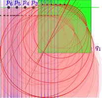
Figure 3.4: The set of disks $D_{1}$, and the construction of $q_{2}$.

Proof:

Let $p_{i}=(-i,0)$, for $i=1,\ldots,n$. Let $M=1+\left\lceil{\log_{2}\Phi}\right\rceil$ and $q_{1}=(n2^{M},-1)$. For a point $p$ on the $x$-axis, and a point $q$ below the $x$-axis and to the right of $p$, let $\ocircle_{\downarrow}^{p}\left({q}\right)$ be the disk whose boundary passes through $p$ and $q$, and its center has the same $x$-coordinate as $p$.

In the $j$th iteration, for $j=2,\ldots,M-1$, Let $x_{j}=n2^{M-j+1}=x(q_{j-1})/2$, and let $y_{j}<0$ be the maximum $y$-coordinate of a point that lies on the intersection of the vertical line $x=x_{j}$ and the disks of $D_{1}\cup\cdots\cup D_{j}$ where

$$D_{j}=\left\{\ocircle_{\downarrow}^{p_{i}}\left({q_{j-1}}\right)\;\middle|\;i=1,\ldots,n\right\},$$

see Figure 3.4 for an illustration of $D_{1}$.

Let $q_{j}=(x_{j},0.99y_{j})$.

Clearly, the point $q_{j}$ lies outside all the disks of $D_{1}\cup\ldots\cup D_{j}$. The construction now continues to the next value of $j$. Let $P=\{p_{1},\ldots,p_{n},q_{2},\ldots,q_{M}\}$. We have that $|P|=n+M-1$.

The minimum distance between any points in the construction is $1$ (i.e., $\left\|p_{1}p_{2}\right\|\bigr{.}$). Indeed $x(q_{M-1})=4n$ and thus $\left\|q_{M-1}p_{1}\right\|\geq 2n$. The diameter of $P$ is $\left\|p_{1}q_{1}\right\|=\sqrt{(n+n2^{M})^{2}+1}\leq 2n2^{M}$. As such, the spread of $P$ is bounded by $\leq n2^{M+1}=\mathcal{O}(n\Phi)$.

For any $i$ and $j$, consider the disk $\ocircle_{\downarrow}^{p_{i}}\left({q_{j}}\right)$. This disk does not contain any point of $p_{1},\ldots,p_{i-1},p_{i+1},\ldots,p_{n}$ since its interior lies below the $x$-axis. By construction it does not contain any point $q_{j+1},\ldots,q_{M-1}$. This disk potentially contains the points $q_{j-1},\ldots,q_{1}$, but observe that for any index $k\in\left\llbracket j-1\right\rrbracket$, we have that

$$\left\|p_{i}q_{k}\right\|=\sqrt{\left({i+n2^{M-k+1}}\right)^{2}+\bigl{(}y(q_{j})\bigr{)}^{2}},$$

which implies that $n2^{M-k+1}\leq\left\|p_{i}q_{k}\right\|<n(2^{M-k+1}+2).$ We thus have that

$$\frac{\left\|p_{i}q_{k}\right\|}{\left\|p_{i}q_{j}\right\|}\geq\frac{n2^{M-k+1}}{n(2^{M-j+1}+2)}=\frac{2^{M-j}\cdot 2^{j-k}}{2^{M-j}+1}=\frac{2^{j-k}}{1+1/2^{M-j}}\geq\frac{2}{1+1/2}=\frac{4}{3}>1+\varepsilon,$$

since $j\in\left\llbracket M-1\right\rrbracket$. Namely, the shortest path in $G$ between $p_{i}$ and $q_{j}$, can not use any of the points $q_{1},\ldots q_{j-1}$. As such, the graph $G$ must contain the edge $p_{i}q_{j}$. This implies that $|E\left({G}\right)|\geq n(M-1)$, which implies the claim.  

3.3.2 A lower bound for triangles

Lemma 3.11.

For any $n>0$, and $\Phi=\Omega(n)$, one can compute a set $P$ of $n+\mathcal{O}(\log\Phi)$ points, with spread $\mathcal{O}(\Phi n)$, and a triangle $\triangle$, such that any $\triangle$-local $(3/2)$-spanner of $P$ requires $\Omega\left({n\log\Phi}\right)$ edges.

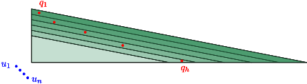
Figure 3.5: An Illustration of the construction of Lemma 3.11.

Proof:

Let $h=\left\lceil{\log_{2}\Phi}\right\rceil$. Let $\triangle$ be the triangle formed by the points $(0,0)$, $(0,1)$ and $(8\Phi h,0)$. The hypotenuse of this triangle lies on the line $\ell\equiv\frac{1}{8\Phi h}x+y=1$, and let $v=\bigl{(}\frac{1}{8\Phi h},1\bigr{)}$ be the vector orthogonal to this line.

For $i\in\left\llbracket h\right\rrbracket$ and $j\in\left\llbracket n\right\rrbracket$, let

$$q_{i}=\bigl{(}2^{i+1},1-i/h\bigr{)}\qquad\text{ and }\qquad u_{j}=\bigl{(}\tfrac{j}{n}-1,-\tfrac{j}{n}\bigr{)},$$

and let $P=\{q_{1},\ldots,q_{h},u_{1},\ldots,u_{n}\}$, see Figure 3.5. Observe that $\mathrm{c{}p}\left({P}\right)=\left\|u_{1}u_{2}\right\|=\sqrt{2}/n$, and as such we have that $\Phi\left({P}\right)=n\cdot\mathrm{diam}\left({P}\right)/\sqrt{2}\leq n(4\Phi+2n)\leq 8\Phi n$, as $\Phi\geq n$. Observe that

$$\left\langle{{q_{i+1}-q_{i}},{v}}\right\rangle=\left\langle{{(2^{i+1},-\tfrac{1}{h})},{\bigl{(}\tfrac{1}{8\Phi h},1\bigr{)}}}\right\rangle\leq\tfrac{4\Phi}{8\Phi h}-\tfrac{1}{h}<0.$$

That is, the points $q_{1},\ldots,q_{i}$ are increasing in distance from $\ell$.

Let $\triangle_{i,j}$ be the homothet of $\triangle$, that has its bottom left corner at $u_{j}$, and its hypotenuse passes through $q_{i}$. By the above, $P(i,j)=\triangle_{i,j}\cap P=\{u_{j},q_{i},q_{i+1},\ldots q_{h}\}$. Any $(1+\varepsilon)$-spanner for $P(i,j)$ must contain the edge $u_{j}q_{i}$. Indeed, we have, for any $k$, that $2^{k+1}\leq\left\|u_{j}q_{k}\right\|\leq 2^{k+1}+3$. As such, any path on a graph induced on $P(i,j)$ from $u_{j}$ to $q_{i}$ that uses (say) a midpoint $q_{k}$, for $k>i$, must have dilation at least

$$\frac{\left\|u_{j}q_{k}\right\|+\left\|q_{k}q_{i}\right\|}{\left\|u_{j}q_{i}\right\|}\geq\frac{2^{k+1}+2^{k}}{2^{i+1}+3}\geq\frac{3\cdot 2^{i+1}}{(1+3/4)2^{i+1}}=\frac{12}{7}>\frac{3}{2}.$$

Thus, any $\triangle$-local $3/2$-spanner for homothets of $\triangle$, must contain the edge $q_{i}u_{j}$, for any $i\in\left\llbracket h\right\rrbracket$ and $j\in\left\llbracket n\right\rrbracket$. Thus, such a spanner must have $\Omega(n\log\Phi)$ edges, as claimed.  

3.4 Local spanners for fat triangles

While local spanners for homothets of an arbitrary convex shape are costly, if we are given a triangle $\triangle$ with the single constraint that $\triangle$ is not too “thin”, then one can construct a $\triangle$-local $t$-spanner with a number of edges that does not depend on the spread of the points. See Figure 3.5 for an illustration of a construction showing that dependency if ”thin” triangles are allowed.

Definition 3.12.

A triangle $\triangle$ is $\alpha$-fat if the smallest angle in $\triangle$ is at least $\alpha$.

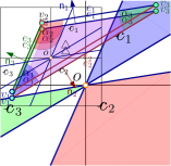
Figure 3.6: For the triangle $\triangle$ with angles $\alpha_{1},\alpha_{2}$, and $\alpha_{3}$ we create the cones $\mathcalb{c}_{1},\mathcalb{c}_{2}$, and $\mathcalb{c}_{3}$.

3.4.1 Construction

The input is a set $P$ of $n$ points in the plane, an $\alpha$-fat triangle $\triangle$, and an approximation parameter $\varepsilon\in(0,1)$. Let $v_{i}$ denote the $i$th vertex of $\triangle$, $\alpha_{i}$ be the adjacent angle, and let $e_{i}$ denote the opposing edge, for $i\in\left\llbracket 3\right\rrbracket$. Let $\mathcalb{c}_{i}=\left\{(p-v_{i})t\;\middle|\;p\in e_{i}\text{ and }t\geq 0\right\}$ denote the cone with an apex at the origin induced by the $i$th vertex of $\triangle$. Let $\mathsf{n}_{i}$ be the outer normal of $\triangle$ orthogonal to $e_{i}$. See Figure 3.6 for an illustration. Let $\mathcal{C}_{i}$ be a minimum size partition of $\mathcalb{c}_{i}$ into cones each with angle in the range $[\beta/2,\beta]$, where $\beta=\varepsilon\alpha/\gamma$, and $\gamma>1$ is a constant to be determined shortly. For each point $p\in P$, and a cone $\mathcalb{c}\in\mathcal{C}_{i}$, let $\mathsf{nn}_{i}\left({p,\mathcalb{c}}\right)$ be the first point in $(P-p)\cap(p+\mathcalb{c})$ ordered by the direction $\mathsf{n}_{i}$ (it is the “nearest-neighbor” to $p$ in $p+\mathcalb{c}$ with respect to the direction $\mathsf{n}_{i}$).

The construction

Let $G$ be the graph over $P$ formed by connecting every point $p\in P$ to $\mathsf{nn}_{i}\left({p,\mathcalb{c}}\right)$, for all $i\in\left\llbracket 3\right\rrbracket$ and $\mathcalb{c}\in\mathcal{C}_{i}$.

3.4.2 Analysis

Lemma 3.13.

Let $p\in P$, $\mathcalb{c}\in\mathcal{C}_{i}$, and $u=\mathsf{nn}_{i}\left({p,\mathcalb{c}}\right)$, and let $q$ be a point in $(P\cap(p+\mathcalb{c}))\setminus\{p,u\}$. We have that $\left\|pu\right\|+(1+\varepsilon)\left\|qu\right\|\leq(1+\varepsilon)\left\|pq\right\|$ and $\left\|qu\right\|\leq\left\|pq\right\|.$

Figure 3.7: The case that $\left\|pq\right\|\leq\left\|pu\right\|$ in Lemma 3.13. The vector used to determine $\mathsf{nn}_{i}\left({p,\mathcalb{c}}\right)$ is shown in red, and denoted $\mathsf{n}$

Proof:

Consider the triangle $\Delta pqu$ and denote the angles at $p,q,$ and $u$ by $\sphericalangle p,\sphericalangle q$, and $\sphericalangle u$ respectively. Since the angle of $\mathcalb{c}$ is smaller than $60$ degrees (for an appropriate choice of $\gamma$), we have that $\left\|qu\right\|\leq\max\{\left\|pu\right\|,\left\|pq\right\|\}$.

Consider the case that $\left\|pq\right\|\leq\left\|pu\right\|$, illustrated in Figure 3.7. Observe that $\sphericalangle u\leq\sphericalangle q$. As such $\sphericalangle u\leq\pi/2$. Furthermore, $\sphericalangle u\geq\alpha\gg\varepsilon\alpha/\gamma=\beta\geq\sphericalangle p$. Similarly, $\sphericalangle q\in[\alpha,\pi-\alpha]$. By the $1$-Lipshitz of $\sin$, and as $\sin x\approx x$, for small $x$, and for $\gamma$ sufficiently large, we have that

$$\sin(\sphericalangle q+\sphericalangle p)\in[1-\varepsilon/4,1+\varepsilon/4]\sin\sphericalangle q\qquad\text{and}\qquad\sin\sphericalangle p\leq(\varepsilon/4)\sin\sphericalangle u.$$

As such, by the law of sines, we have that $\frac{\left\|qu\right\|}{\sin{\sphericalangle p}}=\frac{\left\|pq\right\|}{\sin{\sphericalangle u}}=\frac{\left\|pu\right\|}{\sin{\sphericalangle q}}.$ This implies that

$$\left\|pu\right\|+(1+\varepsilon)\left\|qu\right\|=\left({\frac{\sin{\sphericalangle q}}{\sin{\sphericalangle u}}+(1+\varepsilon)\frac{\sin{\sphericalangle p}}{\sin{\sphericalangle u}}}\right)\left\|pq\right\|.$$

Observe, by the above that

$$\frac{\sin{\sphericalangle q}}{\sin{\sphericalangle u}}+(1+\varepsilon)\frac{\sin{\sphericalangle p}}{\sin{\sphericalangle u}}\leq\frac{\sin{\sphericalangle q}}{\sin{\left({\sphericalangle p+\sphericalangle q}\right)}}+(1+\varepsilon)\frac{\varepsilon}{4}\leq\frac{\sin{\sphericalangle q}}{(1-\varepsilon/4)\sin{\left({\sphericalangle q}\right)}}+(1+\varepsilon)\frac{\varepsilon}{4}\leq 1+\varepsilon.$$

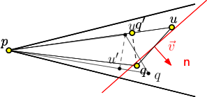
Figure 3.8: The case that $\left\|pq\right\|>\left\|pu\right\|$ in Lemma 3.13.

The other possibility is that $\left\|pq\right\|>\left\|pu\right\|$, illustrated in Figure 3.8. Let $u^{\prime}$ be the projection of $u$ to $pq$. Observe that

$$\left\|uu^{\prime}\right\|=\left\|pu^{\prime}\right\|\tan\sphericalangle p\leq 2\beta\left\|pu^{\prime}\right\|\leq(\varepsilon/8)\left\|pu^{\prime}\right\|.$$

Observe that $\cos\sphericalangle p\geq 1-(\sphericalangle p)^{2}/2\geq 1-\varepsilon^{2}/8$ as $\sphericalangle p$ is an angle smaller than (say) $\varepsilon/16$. As such $1/\cos\sphericalangle p\leq 1+\varepsilon^{2}/4$. This implies that $\left\|pu\right\|\leq{\left\|pu^{\prime}\right\|}/{\cos\sphericalangle p}\leq(1+\varepsilon^{2}/4)\left\|pu^{\prime}\right\|.$ We thus have that

$$\tau =\left\|pu\right\|+(1+\varepsilon)\left\|qu\right\|\leq(1+\varepsilon^{2}/4)\left\|pu^{\prime}\right\|+(1+\varepsilon)\left({\Bigl{.}\left\|uu^{\prime}\right\|+\left\|u^{\prime}q\right\|}\right)$$

$$\leq\bigl{(}1+\varepsilon^{2}/4+(1+\varepsilon)\varepsilon/8\bigr{)}\left\|pu^{\prime}\right\|+(1+\varepsilon)\left\|u^{\prime}q\right\|\leq(1+\varepsilon)\left\|pq\right\|.$$

 

Lemma 3.14.

Let $\triangle$ be a triangle that contains two points $p,q$. Then, there is a homothet $\triangle^{\prime}\subseteq\triangle$ of $\triangle$, such that one of these points is a vertex of $\triangle^{\prime}$, and the other point lies on a facing edge of $\triangle^{\prime}$.

Proof:

This follows by the same shrinking argument as Lemma 3.3, with the addition of a single step. When a homothet $\triangle^{\prime}$ with $p,q\in\partial\triangle^{\prime}$ is found, if neither point is on a vertex, we “push” the only edge that does not contain one of the points towards the vertex $v$ opposite of it (this the same mapping described in Lemma 3.3 with center $v$), until one of the points, say $p$ lies on the edge. $p$ now lies on two edges, meaning, at a vertex, while $q$ lies on the only remaining edge which must be opposite of that vertex. See Figure 3.9.  

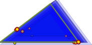
Figure 3.9: An illustration of the shrinking process of Lemma 3.14. The three left figures illustrates the process of Lemma 3.3, for the case that the convex region $\mathcal{C}$ is a triangle, and the rightmost figure is the additional final step.

Local spanner property

Lemma 3.15.

Let $\triangle^{\prime}$ be a homothet of $\triangle$. For any two points $p,q\in P\cap\triangle^{\prime}$, we have a $(1+\varepsilon)$-path in $G^{\prime}=G\cap{\triangle^{\prime}}$.

Proof:

Consider the closest pair $p,q\in P\cap\triangle$. They must be connected directly in $G^{\prime}$, as otherwise there is a point $u\in P^{\prime}=P\cap\triangle^{\prime}$ in the cone containing the segment $pq$, such that $pu\in E\left({G^{\prime}}\right)$. But then, by Lemma 3.13, we have $\left\|pu\right\|+(1+\varepsilon)\left\|qu\right\|\leq(1+\varepsilon)\left\|pq\right\|,$ which implies that either $pu$ or $qu$ are the closest pair, which is a contradiction.

For any other pair $p,q\in P^{\prime}$ we have from Lemma 3.14 that there exists a homothet $\triangle^{\prime\prime}\subseteq\triangle^{\prime}$ with one of the two points, say $p$, at a vertex, and the other on the opposite edge. We therefore have a cone $\mathcalb{c}$ with apex at $p$ such that $q\in\mathcalb{c}\cap\triangle^{\prime\prime}$. If $pq$ is an edge in $G$ then we are done. Otherwise, we have a vertex $u\in\mathcalb{c}$ such that $pu$ is an edge in $G$, and by Lemma 3.13 we have $\left\|qu\right\|\leq\left\|pq\right\|$, which, by induction, means that there exists a $(1+\varepsilon)$ path between $u$ and $q$ in $G$. Lemma 3.13 now implies that $\left\|pu\right\|+(1+\varepsilon)\left\|qu\right\|\leq(1+\varepsilon)\left\|pq\right\|$. Thus, there is a $(1+\varepsilon)$ path between $p$ and $q$ in $G^{\prime}$, as stated.  

Size and running time

Theorem 3.16.

Let $P$ be a set of $n$ points in the plane, and let $\varepsilon\in(0,1)$ be an approximation parameter. The above algorithm computes a $\triangle$-local $(1+\varepsilon)$-spanner $G$ for an $\alpha$-fat triangle $\triangle$. The construction time is $\mathcal{O}\left({(\alpha\varepsilon)^{-1}n\log n}\right)$, and the spanner $G$ has $\mathcal{O}\left({(\alpha\varepsilon)^{-1}n\bigr{.}}\right)$ edges.

Proof:

The local-spanning property is proven in Lemma 3.15, and we are only left with bounding the size and the running time of the algorithm. The bound on the size is immediate from the construction, as every point $p$ is the apex of $\mathcal{O}\left({\frac{2\pi}{\varepsilon\alpha}}\right)$ cones, each giving rise to a single edge incident to $p$. The construction time is bounded by the construction time for a $\theta$-graph with cone size $\alpha\varepsilon$, which is $\mathcal{O}\left({(\alpha\varepsilon)^{-1}n\log n}\right)$ ([Cla87]).  

3.5 A local spanner for nice polygons

3.5.1 A good jump for narrow trapezoids

As a reminder, a trapezoid is a quadrilateral with two parallel edges, known as its bases. The other two edges are its legs. For $\varepsilon\in(0,1/4)$, a trapezoid $T$ is $\varepsilon$-narrow if the length of each of its legs is at most $\varepsilon\cdot\mathrm{diam}\left({T}\right)$.

Lemma 3.17.

Let $\varepsilon\in(0,1)$ be some parameter, and $\vartheta=\varepsilon/16$. Let $X,Y$ be two points sets that are $\vartheta$-semi separated and $\vartheta$-angularly separated (see Definition 2.7), and let $T$ be a $\vartheta$-narrow trapezoid, with two points $p\in X$ and $q\in Y$ lying on the two legs of $T$. Then, one can compute a homothet $T^{\prime}\subseteq T$ of $T$, such that:

1. There are two points $p^{\prime}\in X$ and $q^{\prime}\in Y$, such that $p^{\prime}q^{\prime}$ is an edge of the $T$-Delaunay triangulation of $X\cup Y$.

2. We have that $(1+\varepsilon)\left\|pp^{\prime}\right\|+\left\|p^{\prime}q^{\prime}\right\|+(1+\varepsilon)\left\|q^{\prime}q\right\|\leq(1+\varepsilon)\left\|pq\right\|$.

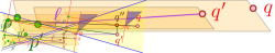
(i)       (ii)       (iii)

Figure 3.10: Illustration of the settings in the proof of Lemma 3.17. Left: A $\vartheta$-narrow trapezoid with $p$ and $q$ on its legs. Center: $p$ and $q$ are $\vartheta$-semi separated and $\vartheta$-angularly separated. Right: The triangle of all the points of the trapezoids that their nearest point on $pq$ is $q$.

Proof:

Let $\mathcal{D}=\mathcal{D}_{T}(X\cup Y)$. Claim 3.4 implies that $\mathcal{D}\cap T$ is connected. Thus, there is a path in $\mathcal{D}\cap T$ between $p$ and $q$, and thus, there must be an edge $p^{\prime}q^{\prime}$ along this path with $p^{\prime}\in X$ and $q^{\prime}\in Y$. This implies part (I).

Let $\ell=\left\|p^{\prime}q^{\prime}\right\|$. Assume for concreteness that $\left\|pp^{\prime}\right\|\leq\mathrm{diam}\left({X}\right)\leq\vartheta\mathsf{d}\left({X,Y}\right)\leq\vartheta\ell\leq\vartheta\mathcalb{d}$, where $\mathcalb{d}=\mathrm{diam}\left({T}\right)$. Let $q^{\prime\prime}$ be the closest point on $pq$ to $q^{\prime}$.

We first consider the case that $q^{\prime\prime}\in\mathrm{int}\left({pq}\right)$. We have that

$$\left\|pq^{\prime\prime}\right\|=\left\|pq^{\prime}\right\|\cos\angle q^{\prime}pq\geq\bigl{(}\left\|p^{\prime}q^{\prime}\right\|-\left\|pp^{\prime}\right\|\bigr{)}\cos\angle q^{\prime}pq\geq(1-\vartheta)\ell\cdot(1-\vartheta^{2}/2)\geq(1-2\vartheta)\ell,$$

since $\cos\vartheta\geq 1-\vartheta^{2}/2$, for $\vartheta<1/2$. Similar argumentation implies that $\left\|pq^{\prime\prime}\right\|\leq(1+\vartheta)\ell$. As such, we have

$$\left\|q^{\prime}q^{\prime\prime}\right\|\leq(1+\vartheta)\ell\sin\angle p^{\prime}pq^{\prime}\leq 2\vartheta\ell.$$

Thus, we have that

$$\left\|qq^{\prime}\right\|\leq\left\|qq^{\prime\prime}\right\|+\left\|q^{\prime\prime}q^{\prime}\right\|\leq\left\|pq\right\|-\left\|pq^{\prime\prime}\right\|+2\vartheta\ell\leq\left\|pq\right\|-(1-2\vartheta)\ell+2\vartheta\ell\leq\left\|pq\right\|-\ell.$$

Thus, we have that

$$(1+\varepsilon)\left\|pp^{\prime}\right\|+\left\|p^{\prime}q^{\prime}\right\|+(1+\varepsilon)\left\|q^{\prime}q\right\|\leq(1+\varepsilon)\vartheta\ell+\ell+(1+\varepsilon)\bigl{(}\left\|pq\right\|-\ell\bigr{)}$$

$$\qquad=(1+\varepsilon)\left\|pq\right\|+(1+\varepsilon)\vartheta\ell+\ell-(1+\varepsilon)\ell\leq(1+\varepsilon)\left\|pq\right\|,$$

for $\vartheta\leq\varepsilon/2$. Which establish the claim in this case.

The case that $q^{\prime\prime}=p$ is impossible, because of the angular separation property. Thus, the only remaining possibility is that $q^{\prime\prime}=q$. This however implies that $q^{\prime}$ must be in the triangle of all the points of the trapezoids that their nearest point on $pq$ is $q$. The diameter of this triangle is bounded by the length of the leg of the trapezoid, which is bounded by $\vartheta\,\mathcalb{d}$. Namely, we have $\left\|qq^{\prime}\right\|\leq\vartheta\mathcalb{d}$. Similarly, we have $(1-2\vartheta)\mathcalb{d}\leq\left\|pq\right\|\leq(1+2\vartheta)\mathcalb{d}.$ Since $\left\|pp^{\prime}\right\|,\left\|qq^{\prime}\right\|\leq\vartheta\mathcalb{d}$, it follows that

$$(1-4\vartheta)\mathcalb{d}\leq\ell\leq(1+4\vartheta)\mathcalb{d}.$$

As such, for $\vartheta\leq\varepsilon/8$ and $\varepsilon\leq 1$, we have

$$(1+\varepsilon)\left\|pp^{\prime}\right\|+\ell+(1+\varepsilon)\left\|q^{\prime}q\right\|\leq 4\vartheta\mathcalb{d}+(1+4\vartheta)\mathcalb{d}=(1+8\vartheta)\mathcalb{d}\leq(1+\varepsilon)\left\|pq\right\|.$$

 

3.5.2 Breaking a nice polygon into narrow trapezoids

For a convex polygon $\mathcal{C}$, its sensitivity, denoted by $\mathrm{sen}\left({\mathcal{C}}\right)$, is the minimum distance between any two non-adjacent edges (this quantity is no bigger than the length of the shortest edge in the polygon). A convex polygon $\mathcal{C}$ is $t$-nice, if the outer angle at any vertex of the polygon is at least $2\pi/t$, and the length of the longest edge of $\mathcal{C}$ is $\mathcal{O}(\mathrm{sen}\left({\mathcal{C}}\right))$. As an example, a $k$-regular polygon is $k$-nice.

Lemma 3.18.

Let $t$ be a positive integer. Given a $t$-nice polygon $\mathcal{C}$, and a parameter $\vartheta$, one can cover it by a set $\mathcal{T}$ of $\mathcal{O}(t^{4}/\vartheta^{3})$ $\vartheta$-narrow trapezoids, such that for any two points $p,q\in\partial\mathcal{C}$ that belong to two edges of $\mathcal{C}$ that are not adjacent, there exists a narrow trapezoid $T\in\mathcal{T}$, such that $p$ and $q$ are located on two different short legs of $T$.

Proof:

We show a somewhat suboptimal but simple construction. A $t$-nice polygon has at most $t$ edges. Let $\psi$ be the sensitivity of $\mathcal{C}$, and place a minimum set of points $P$ on the boundary of $\mathcal{C}$, which includes all the vertices of $\mathcal{C}$, and such that the distance between any consecutive pair of points is in the range $[c_{1},2c_{1}]$, where $c_{1}=\vartheta\psi/c_{2}$, for some sufficiently large constant $c_{2}$. In particular, let $M=\max_{e\in E\left({\mathcal{C}}\right)}\left\lceil{\|e\|/c_{1}}\right\rceil=\mathcal{O}(1/\vartheta)$.

In addition, place $c_{3}t$ equally spaced points between any two consecutive points of $P$, where $c_{3}$ is a constant to be determined shortly. Let $Q$ be the set resulting from $P$ after adding all these points.

Figure 3.11: The points of $P$ (round), and all the points added to $P$ in order to create $Q$ (square). On the right, a “vertical” decomposition induced by one of the directions of $P\times Q$.

We have that $|P|=\mathcal{O}(t/\vartheta)$ and $|Q|=\mathcal{O}(t^{2}/\vartheta)$. For a direction $v$, let $\mathcal{T}_{v}$ be the decomposition into trapezoids formed by shooting rays from inside $\mathcal{C}$ in the direction of $v$ (or $-v$) from all the points of $P$, see Figure 3.11. Let $\mathcal{T}_{v}^{\prime}$ be the set resulting from throwing away trapezoids with legs that lie on adjacent edges. It is easy to verify that all the trapezoids of $\mathcal{T}_{v}^{\prime}$ are $\vartheta$-narrow. Let $U$ be the set of all directions induced by pairs of points of $P\times Q$, and let $\mathcal{T}=\cup_{u\in U}\mathcal{T}_{u}^{\prime}$. We have that $|\mathcal{T}|=\mathcal{O}(|P|\cdot|U|)=\mathcal{O}(|P|^{2}|Q|)=\mathcal{O}(t^{4}/\vartheta^{3})$.

Consider any two points $p,q$ on non-adjacent edges of $\mathcal{C}$, and let $p_{1},p_{2}$ be the two adjacent points of $P$ such that $p\in p_{1}p_{2}$. Now, let $q_{1},q_{2}$ be the adjacent points of $Q$ such that $q\in q_{1}q_{2}$. We assume that $p_{1},p_{2},q_{1},q_{2}$ are in this clockwise order along the boundary of $\mathcal{C}$.

Observe that when we project the interval $p_{1}p_{2}$, to the line induced by $q_{1}q_{2}$, in the direction $\overrightarrow{p_{1}q_{2}}$, the projected interval contains $q_{1}q_{2}$. The last claim is intuitively obvious, but requires some work to see formally. The minimum height of a triangle involving three vertices of $\mathcal{C}$ is formed by three consecutive vertices. In the worst case, this is an isosceles triangle with sidelength $\psi$ and base angle $\pi/t$. As such, the height of such a triangle is $h=\psi\sin(\pi/t)\geq\psi/t$.

Figure 3.12: The height of the triangle $\triangle p_{1}p_{2}q_{2}$ is minimized as $q_{2}$ and $p_{1}$ are moved to vertices of $\mathcal{C}$.

The height of the triangle $\triangle p_{1}p_{2}q_{2}$ is minimized when $p_{1}$ or $p_{2}$ is a vertex of $\mathcal{C}$, and $q_{2}$ is at a vertex of $\mathcal{C}$, see Figure 3.12. Assume, for concreteness, that $p_{1}$ is a vertex of $\mathcal{C}$, and observe that $\left\|p_{1}p_{2}\right\|\geq\|e\|/M$, where $e$ is the edge of $\mathcal{C}$ containing this segment. Using similar triangles, it is straightforward to show that the height of this triangle is at least $h^{\prime}=h/M=\Omega(\varepsilon\psi/t)$. The quantity $h^{\prime}$ is a lower bound on the length of the projection of $p_{1}p_{2}$ on the line spanned by $q_{1}q_{2}$. However, $\left\|q_{1}q_{2}\right\|\leq 2c_{1}/c_{3}t=\mathcal{O}(\vartheta\psi/c_{3}t)<h^{\prime}$, by picking $c_{3}$ to be sufficiently large constant.

This readily implies that the trapezoid induced by the direction $u=\overrightarrow{p_{1}q_{2}}$ in $\mathcal{T}_{u}^{\prime}$ that contains $p$ on its leg, contains $q$ on its other leg.  

3.5.3 Constructing the local spanner for nice polygons

Theorem 3.19.

Let $\mathcal{C}$ be a $k$-nice convex polygon, $P$ be a set of $n$ points in the plane, and let $\varepsilon\in(0,1)$ be a parameter. Then, one can construct a $\mathcal{C}$-local $(1+\varepsilon)$-spanner of $P$. The construction time is $\mathcal{O}\left({\bigl{.}({k^{4}}/{\varepsilon^{6}})n\log^{2}n}\right)$, and the resulting graph has $\mathcal{O}\left({\bigl{.}({k^{4}}/{\varepsilon^{6}})n\log n}\right)$ edges. In particular these bounds hold if $\mathcal{C}$ is a $k$-regular polygon.

Proof:

Let $\vartheta=\varepsilon/c_{4}$, for $c_{4}$ sufficiently large constant. We construct $\bm{\Delta}$, a family of triangles induced by a vertex of $\mathcal{C}$, and an non-adjacent edge of $\mathcal{C}$. This family has $\mathcal{O}(k^{2})$ triangles. Each such triangle is $\Omega(1/k)$-fat, and for each such triangle we construct the $(1+\vartheta)$-spanner of Theorem 3.16 for P. Next, we cover $\mathcal{C}$ by a set $\mathcal{T}$ of $k^{\prime}=\mathcal{O}(k^{4}/\vartheta^{3})$ $\vartheta$-narrow trapezoids using Lemma 3.18.

We compute an $\vartheta$-angular $(1/\vartheta)$-SSPD $\mathcal{W}$ decomposition of $P$ using Corollary 2.9 – the total weight of the decomposition is $w=\mathcal{O}\left({n\vartheta^{-3}\log n}\right)$. For each pair $\{X,Y\}\in\mathcal{W}$, and each trapezoid $T\in\mathcal{T}$, we compute the $T$-Delaunay triangulation of $X\cup Y$.

Let $G$ denote the union of all these graphs. We claim that it is the desired spanner. The construction time is

$$\mathcal{O}((k^{3}/\vartheta)n\log n+k^{\prime}w\log n)=\mathcal{O}\left({\frac{k^{3}}{\vartheta}n\log n+\frac{k^{4}}{\vartheta^{3}}\cdot\frac{n}{\vartheta^{3}}\log n\cdot\log n}\right)=\mathcal{O}\left({\frac{k^{4}}{\vartheta^{6}}n\log^{2}n}\right),$$

and the resulting graph has $\mathcal{O}\left({\bigl{.}({k^{4}}/{\vartheta^{6}})n\log n}\right)$ edges.

As for correctness, consider a homothet $\mathcal{C}^{\prime}$ of $\mathcal{C}$ that contains two points $p,q\in P$. By Lemma 3.3, there is a homothet $\mathcal{C}^{\prime\prime}\subseteq\mathcal{C}^{\prime}$ of $\mathcal{C}$ such that $p,q\in\partial\mathcal{C}^{\prime\prime}$. There are two possibilities:

(A) The point $p$ is on a vertex of $\mathcal{C}^{\prime\prime}$ and $q$ is on an edge. In this case, the vertex and the edge induce a fat triangle, that is a homothet of a triangle $\triangle\in\bm{\Delta}$. Since the graph $G$ contains a $\triangle$-local $(1+\varepsilon)$-spanner for $P$, it follows readily that $G$ is a $(1+\varepsilon)$-spanner for these points, and the path is strictly inside $\mathcal{C}^{\prime\prime}$.

(B) The points $p$ and $q$ are on two non-adjacent edges of $\mathcal{C}^{\prime\prime}$. Then, there is an $\vartheta$-narrow trapezoid $T^{\prime}$ that has $p$ and $q$ on its two legs, and a homothet of $T^{\prime}$, denoted by $T$, is in $\mathcal{T}$. There is a pair $\{X,Y\}\in\mathcal{W}$ that is $(1/\vartheta)$-semi separated (and $\vartheta$-angularly separated), such that $p\in X$ and $q\in Y$. By Lemma 3.17, there are two points $p^{\prime}\in X$ and $q^{\prime}\in Y$, such that $p^{\prime}q^{\prime}$ is an edge of the $T$-Delaunay triangulation of $X\cup Y$, and by construction this edge is in $G$. We now use induction on the shortest paths from $p$ to $p^{\prime}$ and from $q$ to $q^{\prime}$ in $G$. By induction, and Lemma 3.17, we have that

$$\mathsf{d}\left({p,q}\right)\leq\mathsf{d}\left({p,p^{\prime}}\right)+\left\|p^{\prime}q^{\prime}\right\|+\mathsf{d}\left({q^{\prime},q}\right)\leq(1+\varepsilon)\left\|pp^{\prime}\right\|+\left\|p^{\prime}q^{\prime}\right\|+(1+\varepsilon)\left\|q^{\prime}q\right\|\leq(1+\varepsilon)\left\|pq\right\|,$$

which implies that the there is $(1+\varepsilon)$-path from $p$ to $q$ inside $\mathcal{C}^{\prime}$.  

Remark 3.20.

For axis-parallel squares Theorem 3.19 implies a local spanner with $\mathcal{O}\left({\varepsilon^{-6}n\log n}\right)$ edges. However, for this special case, the decomposition into narrow trapezoid can be skipped. In particular, in this case, the resulting spanner has $\mathcal{O}(\varepsilon^{-3}n\log n)$ edges. We do not provide the details here, as it is only a minor improvement over the above, and requires quite a bit of additional work – essentially, one has to prove a version of Lemma 3.17 for squares.

4 Weak local spanners for axis-parallel rectangles

4.1 Quadrant separated pair decomposition

For two points $p=(p_{1},\ldots,p_{d})$ and $q=(q_{1},\ldots,q_{d})$ in $\mathbb{R}^{d}$, let $p\prec q$ denotes that $q$ dominates $p$ coordinate-wise. That is $p_{i}<q_{i}$, for all $i$. More generally, let $p<_{i}q$ denote that $p_{i}<q_{i}$. For two point sets $X,Y\subseteq\mathbb{R}^{d}$, we use $X<_{i}Y$ to denote that $\forall x\in X,y\in Y\quad x<_{i}y$. In particular $X$ and $Y$ are $i$-coordinate separated if $X<_{i}Y$ or $Y<_{i}X$. A pair $\{X,Y\}$ is quadrant-separated, if $X$ and $Y$ are $i$-coordinate separated, for $i=1,\ldots,d$.

A quadrant-separated pair decomposition of a point set $P\subseteq\mathbb{R}^{d}$, is a pair decomposition (see Definition 2.2) $\mathcal{W}=\bigl{\{}\{X_{1},Y_{1}\},\ldots,\{X_{s},Y_{s}\}\bigr{\}}$ of $P$, such that $\{X_{i},Y_{i}\}$ are quadrant-separated for all $i$.

Lemma 4.1.

Given a set $P$ of $n$ points in $\mathbb{R}$, one can compute, in $\mathcal{O}(n\log n)$ time, a QSPD of $P$ with $\mathcal{O}(n)$ pairs, and of total weight $\mathcal{O}(n\log n)$.

Proof:

If $P$ is a singleton then there is nothing to do. If $P=\{p,q\}$, then the decomposition is the pair formed by the two singleton points.

Otherwise, let $x$ be the median of $P$, such that $P_{\leq x}=\left\{p\in P\;\middle|\;p\leq x\right\}$ contains exactly $\left\lceil{n/2}\right\rceil$ points, and $P_{>x}=P\setminus P_{\leq x}$ contains $\left\lfloor{n/2}\right\rfloor$ points. Construct the pair $\Xi=\{P_{\leq x},P_{>x}\}$, and compute recursively a QSPDs $\mathcal{Q}_{\leq x}$ and $\mathcal{Q}_{>x}$ for $P_{\leq x}$ and $P_{>x}$, respectively. The desired QSPD is $\mathcal{Q}_{\leq x}\cup\mathcal{Q}_{>x}\cup\{\Xi\}.$ The bounds on the size and weight of the desired QSPD are immediate.  

Lemma 4.2.

Given a set $P$ of $n$ points in $\mathbb{R}^{d}$, one can compute, in $\mathcal{O}(n\log^{d}n)$ time, a QSPD of $P$ with $\mathcal{O}(n\log^{d-1}n)$ pairs, and of total weight $\mathcal{O}(n\log^{d}n)$.

Proof:

The construction algorithm is recursive on the dimensions, using the algorithm of Lemma 4.1 in one dimension.

The algorithm computes a value $\alpha_{d}$ that partitions the values of the points’ $d$th coordinates roughly equally (and is distinct from all of them), and let $h$ be a hyperplane parallel to the first $d-1$ coordinate axes, and having value $\alpha_{d}$ in the $d$th coordinate.

Let $P_{\uparrow}$ and $P_{\downarrow}$ be the subset of points of $P$ that are above and below $h$, respectively. The algorithm recursively computes QSPDs $\mathcal{Q}_{\uparrow}$ and $\mathcal{Q}_{\downarrow}$ for $P_{\uparrow}$ and $P_{\downarrow}$, respectively. Next, the algorithm projects the points of $P$ on $h$, let $P^{\prime}$ be the resulting $d-1$ dimensional point set (after we ignore the $d$th coordinate), and recursively computes a QSPD $\mathcal{Q}^{\prime}$ for $P^{\prime}$.

For a point set $X^{\prime}\subseteq P^{\prime}$, let $\mathrm{lift}\left({X^{\prime}}\right)$ be the subset of points of $P$ whose projection on $h$ is $X^{\prime}$. The algorithm now computes the set of pairs

$$\widehat{\mathcal{Q}}=\left\{\Bigl{.}\{\mathrm{lift}\left({X^{\prime}}\right)\cap P_{\uparrow},\mathrm{lift}\left({Y^{\prime}}\right)\cap P_{\downarrow}\},\,\,\{\mathrm{lift}\left({X^{\prime}}\right)\cap P_{\downarrow},\mathrm{lift}\left({Y^{\prime}}\right)\cap P_{\uparrow}\}\;\middle|\;\{X^{\prime},Y^{\prime}\}\in\mathcal{Q}^{\prime}\right\}.$$

The desired QSPD is $\widehat{\mathcal{Q}}\cup\mathcal{Q}_{\uparrow}\cup\mathcal{Q}_{\downarrow}$.

To observe that this is indeed a QSPD, observe that all the pairs in $\mathcal{Q}_{\uparrow},\mathcal{Q}_{\downarrow}$ are quadrant separated by induction. As for pairs in $\widehat{\mathcal{Q}}$, they are quadrant separated in the first $d-1$ coordinates by induction on the dimension, and separated in the $d$ coordinate since one side of the pair comes from $P_{\uparrow}$, and the other side from $P_{\downarrow}$.

As for coverage, consider any pair of points $p,q\in P$, and observe that the claim holds by induction if they are both in $P_{\uparrow}$ or $P_{\downarrow}$. As such, assume that $p\in P_{\uparrow}$ and $q\ni P_{\downarrow}$. But then there is a pair $\{X^{\prime},Y^{\prime}\}\in\mathcal{Q}^{\prime}$ that separates the two projected points in $h$, and clearly one of the two lifted pairs that corresponds to this pair quadrant-separates $p$ and $q$ as desired.

The number pairs in the decomposition is $N(n,d)=2N(n,d-1)+2N\left({n/2,d}\right)$ with $N(n,1)=\mathcal{O}(n)$. The solution to this recurrence is $N(n,d)=\mathcal{O}(n\log^{d-1}n)$. The total weight of the decomposition is $W(n,d)=2W(n,d-1)+2W\left({n/2,d}\right)$ with $W(n,1)=\mathcal{O}(n\log n)$. The solution to this recurrence is $W(n,d)=\mathcal{O}(n\log^{d}n)$. Clearly, this also bounds the construction time.  

4.2 Weak local spanner for axis parallel rectangles

For a parameter $\delta\in(0,1)$, and an interval $I=[b,c]$, let $(1-\delta)I=[t-(1-\delta)r,t+(1-\delta)r]$, where $t=(b+c)/2$, and $r=(c-b)/2$, be the shrinking of $I$ by a factor of $1-\delta$.

Let $\mathcal{R}$ be the set of all axis parallel rectangles in the plane. For a rectangle ${R}\in\mathcal{R}$, with ${R}=I\times J$, let $(1-\delta){R}=(1-\delta)I\times(1-\delta)J$ denote the rectangle resulting from shrinking ${R}$ by a factor of $1-\delta$.

Definition 4.3.

Given a set $P$ of $n$ points in the plane, and parameters $\varepsilon,\delta\in(0,1)$, a graph $G$ is a $(1-\delta)$-local $(1+\varepsilon)$-spanner for rectangles, if for any axis-parallel rectangle ${R}$, we have that $G\cap{{R}}$ is a $(1+\varepsilon)$-spanner for all the points in $\bigl{(}(1-\delta){R}\bigr{)}\cap P$.

Observe that rectangles in $\mathcal{R}$ might be quite “skinny”, so the previous notion of shrinkage used before is not useful in this case.

4.2.1 Construction for a single quadrant separated pair

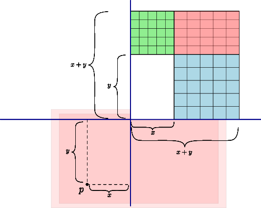
Figure 4.1: The construction of the grid $\mathsf{K}(p,\Xi)$ for a point $p=(-x,-y)$ and a pair $\Xi$.

Consider a pair $\Xi=\{X,Y\}$ in a QSPD of $P$. The set $X$ is quadrant-separated from $Y$. That is, there is a point $c_{\Xi}$, such that $X$ and $Y$ are contained in two opposing quadrants in the partition of the plane formed by the vertical and horizontal line through $c_{\Xi}$.

For simplicity of exposition, assume that $c_{\Xi}=(0,0)$, and $X\prec(0,0)\prec Y$. That is, the points of $X$ are in the negative quadrant, and the points of $Y$ are in the positive quadrant.

We construct a non-uniform grid $\mathsf{K}(p,\Xi)$ in the square $[0,x+y]^{2}$. To this end, we first partition it into four subrectangles

$$\begin{array}[]{l|l}B_{\nwarrow}=[0,x]\times[y,x+y]&B_{\nearrow}=[x,x+y]\times[y,x+y]\Bigr{.}\\ \hline\cr B_{\swarrow}=[0,x]\times[0,y]&B_{\searrow}=[x,x+y]\times[0,y].\Bigr{.}\\ \end{array}$$

Let $\tau\geq 4/\varepsilon+4/\delta$ be an integer number. We partition each of these rectangles into a $\tau\times\tau$ grid, where each cell is a copy of the rectangle scaled by a factor of $1/\tau$. See Figure 4.1. This grid has $\mathcal{O}(\tau^{2})$ cells. For a cell $\mathsf{C}$ in this grid, let $Y\cap\mathsf{C}$ be the points of $Y$ contained in it. We connect $p$ to the left-most and bottom-most points in $Y\cap\mathsf{C}$. This process generates two edges in the constructed graph for each grid cell (that contains at least two points), and $\mathcal{O}(\tau^{2})$ edges overall.

The algorithm repeats this construction for all the points $p\in X$, and does the symmetric construction for all the points of $Y$.

4.2.2 The construction algorithm

The algorithm computes a QSPD $\mathcal{W}$ of $P$. For each pair $\Xi\in\mathcal{W}$, the algorithm generates edges for $\Xi$ using the algorithm of Section 4.2.1 and adds them to the generated spanner $G$.

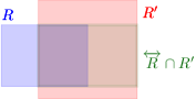
Figure 4.2: Left: The two rectangles ${R}$, ${R}^{\prime}$. Right: In green ${\overleftrightarrow{{R}}}\cap{R}^{\prime}$, the restriction of the slab ${\overleftrightarrow{{R}}}$ to the rectangle ${R}^{\prime}$.

4.2.3 Correctness

For a rectangle ${R}$, let ${\overleftrightarrow{{R}}}=\left\{(x,y)\in\mathbb{R}^{2}\;\middle|\;\exists(x^{\prime},y)\in{R}\right\}$ be its expansion into a horizontal slab. Restricted to a rectangle ${R}^{\prime}$, the resulting set is ${\overleftrightarrow{{R}}}\cap{R}^{\prime}$, depicted in Figure 4.2. Similarly, we denote

$$\updownarrow\!{{R}}=\left\{(x,y)\in\mathbb{R}^{2}\;\middle|\;\exists(x,y^{\prime})\in{R}\right\}.$$

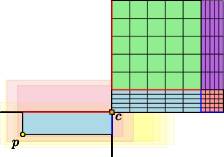
Figure 4.3: An illustration of $\mathsf{K}(p,\Xi)$ with three rectangles and their shrunken version.

Lemma 4.4.

Assume that $\tau\geq\left\lceil{20/\varepsilon+20/\delta}\right\rceil$. Consider a pair $\Xi=\{X,Y\}$ in the above construction, and a point $p=(-x,-y)\in X$ with its associated grid $\mathsf{K}=\mathsf{K}(p,\Xi)$. Consider any axis parallel rectangle ${R}$, such that $p\in(1-\delta){R}=I\times J$, and $(1-\delta){R}$ intersects a cell $\mathsf{C}\in\mathsf{K}$. We have that:

1. If $\mathsf{C}\subseteq(1-\delta){R}$ then $(1-\delta)^{-1}\mathsf{C}\subseteq{R}$.

2. $\mathrm{d{}i{}am}\left({\mathsf{C}}\right)\leq(\varepsilon/4)\mathsf{d}\left({p,\mathsf{C}}\right)$.

3. If $x\geq y$ and $\mathsf{C}\subseteq{R}_{\swarrow}\cup{R}_{\searrow}$ then $(1-\delta)^{-1}\mathsf{C}\subseteq{R}$.

4. If $x\leq y$ and $\mathsf{C}\subseteq{R}_{\swarrow}\cup{R}_{\nwarrow}$ then $(1-\delta)^{-1}\mathsf{C}\subseteq{R}$.

5. If $x\geq y$ and $\mathsf{C}\subseteq{R}_{\nwarrow}$, then $(1-\delta)^{-1}\bigl{(}{\overleftrightarrow{(1-\delta){R}}}\cap\mathsf{C}\bigr{)}\subseteq{R}$.

6. If $x\leq y$ and $\mathsf{C}\subseteq{R}_{\searrow}$, then $(1-\delta)^{-1}\Bigl{(}\updownarrow\!{\bigl{(}(1-\delta){R}\bigr{)}}\cap\mathsf{C}\Bigr{)}\subseteq{R}$.

Proof:

(I) is immediate, (IV) and (VI) follows by symmetry from (III) and (V), respectively.

(II) We have that $\mathrm{d{}i{}am}\left({\mathsf{C}}\right)\leq(x+y)/\tau=\|p\|_{1}/\tau\leq(\varepsilon/4)\mathsf{d}\left({p,\mathsf{C}}\right).$

(III) The width, denoted $\mathsf{wd}\left({\cdot}\right)$, of $(1-\delta){R}$ is at least $x$, as it contains both $p$ and the origin. As such,

$$\bigl{(}\mathsf{wd}\left({{R}}\right)-\mathsf{wd}\left({(1-\delta){R}}\right)\bigr{)}/2\geq 2(x/\tau)\geq 2\mathsf{wd}\left({\mathsf{C}}\right).$$

That is, the width of the “expanded” rectangle ${R}$ is enough to cover $\mathsf{C}$, and a grid cell adjacent to it to the right.

A similar argument about the height shows that ${R}$ covers the region immediately above $\mathsf{C}$ – in particular, the vertical distance from $\mathsf{C}$ to the top boundary of ${R}$ is at least the height of $\mathsf{C}$. This implies that the expanded cell $(1-\delta)^{-1}\mathsf{C}$ is contained in ${R}$, as claimed, as $\delta<1/2$.

(V) We decompose the claim to the two dimensions of the region. Let $B=\bigl{(}{\overleftrightarrow{(1-\delta){R}}}\cap\mathsf{C}\bigr{)}$. Observe that containment in the $x$-axis follows by arguing as in (III). As for the $y$-interval of $B$, observe that it is contained in the $y$-interval of $(1-\delta){R}$, which implies that when expanded by $(1-\delta)^{-1}$, it would be contained in the $y$-interval of ${R}$. Combining the two implies the result.  

Lemma 4.5.

For any axis-parallel rectangle ${R}$, and any two points $p,q\in(1-\delta){R}\cap P$, there exists a $(1+\varepsilon)$-path between $p$ and $q$ in $G$.

Proof:

The proof is by induction over the size of ${R}$ (i.e. area, width, or height). Let $\Xi=\{X,Y\}\in\mathcal{W}$ be the pair in the QSPD that separates $p$ and $q$, let $c$ be the separation point of the pair, and assume for the simplicity of exposition that $p\in X$, $X\prec c\prec Y$, and $c=(0,0)$. Furthermore, assume that $\|p\|_{1}\geq\|q\|_{1}$.

Let $p=(-x,-y)$, and let $\mathsf{C}$ be the grid cell of $\mathsf{K}(p,\Xi)$ that contains $q$. If $\mathsf{C}\subseteq(1-\delta){R}$, then $(1-\delta)^{-1}\mathsf{C}\subseteq{R}$ by Lemma 4.4 (I). As such, let $u$ be the leftmost point in $\mathsf{C}\cap P$. Both $q,u\in(1-\delta)^{-1}\mathsf{C}$, and by induction, there is an $(1+\varepsilon)$-path $\pi$ between them in $G$ (note that the induction applies to the two points, and the “expanded” rectangle $(1-\delta)^{-1}\mathsf{C}$). Since $pu$ is an edge of $G$, prefixing $\pi$ by this edge results in an $(1+\varepsilon)$-path, as $\left\|qu\right\|\leq(\varepsilon/4)\left\|pq\right\|$, by Lemma 4.4 (II) (verifying this requires some standard calculations which we omit).

Otherwise, one need to apply the same argument using the appropriate case of Lemma 4.4. So assume that $x\geq y$ (the case that $y\geq x$ is handled symmetrically). If $\mathsf{C}\subseteq{R}_{\swarrow}\cup{R}_{\searrow}$, then (III) implies that $(1-\delta)^{-1}\mathsf{C}\subseteq{R}$. Which implies that induction applies, and the claim holds.

The remaining case is that $x\geq y$ and $\mathsf{C}\subseteq{R}_{\nwarrow}$. Let $D={\overleftrightarrow{(1-\delta){R}}}\cap\mathsf{C}$. By (V), we have $(1-\delta)^{-1}D\subseteq{R}$. Namely, $q\in(1-\delta){R}\cap\mathsf{C}\subseteq D$, and let $u$ be the lowest point in $\mathsf{C}\cap P$. By construction $pu\in E\left({G}\right)$, $q,u\in D$, $(1-\delta)^{-1}D\subseteq{R}$. As such, we can apply induction to $q$, $u$, and $(1-\delta)^{-1}D$, and conclude that $\mathsf{d}_{G}\left({q,u}\right)\leq(1+\varepsilon)\left\|qu\right\|$. Plugging this into the regular machinery implies the claim.  

Theorem 4.6.

Let $P$ be a set of $n$ points in the plane, and let $\varepsilon,\delta\in(0,1)$ be parameters. The above algorithm constructs, in $\mathcal{O}((1/\varepsilon^{2}+1/\delta^{2})n\log^{2}n)$ time, a graph $G$ with $\mathcal{O}((1/\varepsilon^{2}+1/\delta^{2})n\log^{2}n)$ edges. The graph $G$ is a $(1-\delta)$-local $(1+\varepsilon)$-spanner for axis parallel rectangles. Formally, for any axis-parallel rectangle ${R}$, we have that ${R}\cap P$ is an $(1+\varepsilon)$-spanner for all the points of $\bigl{(}(1-\delta){R}\bigr{)}\cap P$.

Proof:

Computing the QSPD $\mathcal{W}$ takes $\mathcal{O}(n\log^{2}n)$ time. For each pair $\{X,Y\}$ in the decomposition with $m=|X|+|Y|$ points, we need to compute the lowest and leftmost points in $(X\cup Y)\cap\mathsf{C}$, for each cell in the constructed grid. This can readily be done using orthogonal range trees in $\mathcal{O}(\log^{2}n)$ time per query (a somewhat faster query time should be possible by using that offline nature of the queries, etc). This yields the construction time. The size of the computed graph is $\mathcal{O}(\omega\left({\mathcal{W}}\right)\tau^{2})=O\bigl{(}(1/\delta^{2}+1/\varepsilon^{2})n\log^{2}n\bigr{)}$.

The desired local spanner property is provided by Lemma 4.5.  

Appendix A Proof of Lemma 2.8

Restatement of Lemma 2.8. Given a $(1/\varepsilon)$-SSPD $\mathcal{W}$ of $n$ points in the plane, one can refine $\mathcal{W}$ into a $(1/\varepsilon)$-SSPD $\mathcal{W}^{\prime}$, such that each pair $\Xi=\{X,Y\}\in\mathcal{W}^{\prime}$ is contained in a $\varepsilon$-double-wedge $\times_{\Xi}$, such that $X$ and $Y$ are contained in the two different faces of the double wedge $\times_{\Xi}$. We have that $|\mathcal{W}^{\prime}|=\mathcal{O}(|\mathcal{W}|/\varepsilon)$ and $\omega\left({\mathcal{W}^{\prime}}\right)=\mathcal{O}(\omega\left({\mathcal{W}}\right)/\varepsilon)$. The construction time is proportional to the weight of $\mathcal{W}^{\prime}$.

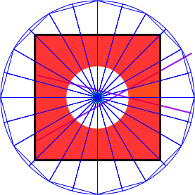
Figure A.1: An illustration of refining the pairs in a SSPD into pairs contained in opposite parts of an $\varepsilon$-double-wedge. $X$ is contained in the green square $\square$, while $Y$ is contained in the red square, and the white gap between them is a result of the separation property. The set of cones with the apex at the center of $\square$ gives us the desired partition as demonstrated by the purple double-wedge.

Proof:

By using Lemma 2.6, we can assume that $\mathcal{W}$ is (say) $(10/\varepsilon)$-separated. Now, the algorithm scans the pairs of $\mathcal{W}$. For each pair $\Xi=\{X,Y\}\in\mathcal{W}$, assume that $\mathrm{d{}i{}am}\left({X}\right)<\mathrm{d{}i{}am}\left({Y}\right)$. Let $\square$ be the smallest axis-parallel square containing $X$, centered at point $o$. Partition the plane around $o$, by drawing $\mathcal{O}(1/\varepsilon)$ lines intersecting $o$ with the angle between any two consecutive lines being at most (say) $\varepsilon/4$, see Figure A.1. This partitions the plane into a set of cones $\mathcal{C}$. For a cone $\mathcalb{c}\in\mathcal{C}$, we show that there exists an $\varepsilon$-double-wedge that contains $X$ in one side, and $Y\cap\mathcalb{c}$ in the other.

To see that, take the double-wedge formed by the cross tangents between $\mathsf{ch}\left({X}\right)$ and $\mathsf{ch}\left({Y\cap\mathcalb{c}}\right)$, where $\mathsf{ch}\left({X}\right)$ denotes the convex-hull of $X$. Assume w.l.o.g that $\square$ has side length 1, and let $c$ be a cone of angle $\varepsilon/4$ with apex $o$, whose angular bisector is a horizontal ray in the positive direction of the $x$ axis. See figure Figure A.2 for an illustration.

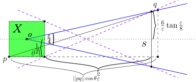
Figure A.2: An illustration of the proof for Lemma 2.8

We would like to find a vertical segment $s$ such that all points of $Y$ lie to its right, with one endpoint on the upper line of $c$, and the other on the lower line of $c$. Using the segments’ height and distance from the right side of $\square$ we will be able to get a bound on the angle of the cross tangents. We first find a segment $s$ with all points of $Y$ to its right. A trivial bound on that distance is given by the segment from, say, the lower left corner of $\square$, denoted $p$, of length $10/\varepsilon$ with its right endpoint on the upper line of $c$, denote this point by $q$. We know that all points of $Y$ lie to the right of $q$ due to the $10/\varepsilon$ separation property of the SSPD. The segment $pq$ creates an angle $\leq\pi/4$ with the $x$-axis (by the choice of the angle of $c$). We therefore get that the $x$-coordinate difference between $\square$ and $q$ is at most $10/\varepsilon\cdot\cos\frac{\pi}{4}-1\leq 7/\varepsilon-1\leq 6/\varepsilon$. So let $s^{\prime}$ be a vertical segment between the upper and lower rays of $c$, with $x$-coordinate distance of $6/\varepsilon-\frac{1}{2}$ from $\square$ (in order to make calculations easier). We get that $s^{\prime}$ is of length $2\cdot\frac{6}{\varepsilon}\tan\frac{\varepsilon}{8}$. Finally, we take $s$ to be a vertical segment of length $\frac{12}{\varepsilon}\tan\frac{\varepsilon}{8}$, with its center on the $x$-axis at a distance of $5/\varepsilon+\frac{1}{2}$ away from $o$. The angle of the $x$-axis and the segment between the lower end of the right side of $\square$ and the upper end of $s$ is now given by:

$$\arctan\left({\frac{\frac{6}{\varepsilon}\tan\frac{\varepsilon}{8}+\frac{1}{2}}{\frac{5}{\varepsilon}}}\right)=\arctan\left({\frac{6}{5}\tan\frac{\varepsilon}{8}+\frac{\varepsilon}{10}}\right)\leq\varepsilon$$

References

- [AB21] Mohammad Ali Abam and Mohammad Sadegh Borouny “Local Geometric Spanners” In Algorithmica 83.12, 2021, pp. 3629–3648 DOI: 10.1007/s00453-021-00860-5
- [ABFG09] Mohammad Ali Abam, Mark Berg, Mohammad Farshi and Joachim Gudmundsson “Region-Fault Tolerant Geometric Spanners” In Discret. Comput. Geom. 41.4, 2009, pp. 556–582 DOI: 10.1007/s00454-009-9137-7
- [AH12] M.. Abam and S. Har-Peled “New Constructions of SSPDs and their Applications” In Comput. Geom. Theory Appl. 45.5–6, 2012, pp. 200–214 DOI: 10.1016/j.comgeo.2011.12.003
- [AMS99] S. Arya, D.. Mount and M. Smid “Dynamic algorithms for geometric spanners of small diameter: Randomized solutions” In Comput. Geom. Theory Appl. 13.2, 1999, pp. 91–107 DOI: https://doi.org/10.1016/S0925-7721(99)00014-0
- [CD85] L Paul Chew and Robert L Dyrsdale III “Voronoi diagrams based on convex distance functions” In Proc. 1st Annu. Sympos. Comput. Geom. (SoCG), 1985, pp. 235–244
- [Cla87] Kenneth L. Clarkson “Approximation Algorithms for Shortest Path Motion Planning (Extended Abstract)” In Proceedings of the 19th Annual ACM Symposium on Theory of Computing, 1987, New York, New York, USA ACM, 1987, pp. 56–65 DOI: 10.1145/28395.28402
- [Har11] S. Har-Peled “Geometric Approximation Algorithms” 173, Math. Surveys & Monographs Boston, MA, USA: Amer. Math. Soc., 2011 DOI: 10.1090/surv/173
- [LNS02] Christos Levcopoulos, Giri Narasimhan and Michiel H.. Smid “Improved Algorithms for Constructing Fault-Tolerant Spanners” In Algorithmica 32.1, 2002, pp. 144–156 DOI: 10.1007/s00453-001-0075-x
- [Luk99] Tamás Lukovszki “New Results of Fault Tolerant Geometric Spanners” In Algorithms and Data Structures, 6th International Workshop, WADS ’99, Vancouver, British Columbia, Canada, August 11-14, 1999, Proceedings 1663, Lecture Notes in Computer Science Springer, 1999, pp. 193–204 DOI: 10.1007/3-540-48447-7“˙20
- [NS07] Giri Narasimhan and Michiel H.. Smid “Geometric spanner networks” Cambridge University Press, 2007