An Accurate Analytic Model for Traveling Wave Tube Dispersion Relation

Abstract

We construct an analytical model for the dispersion of the hot modes in a traveling wave tube (TWT) based on the Lagrangian field theory, upgrading its constants to be frequency-dependent. The frequency dependence of the parameters of the TWT slow wave structure (SWS) is recovered from full-wave simulations by standard software (e.g., CST). We applied the model to study the hot modes of a helical-based TWT and found an excellent agreement between the results from our model and those from particle in cell (PIC) simulations. Our additional studies show that the proposed approach can be applied to various SWS geometries.

I Introduction

Vacuum electron devices (VEDs) are used widely for radar and satellite communications applications for several decades due to their high power operational capabilities and reliability[1, 2]. VEDs operation is based on the synchronous interaction of an electromagnetic (EM) wave in a slow wave structure (SWS) with the electron beam [3, 4].

We advance here an analytical model of traveling wave tubes (TWTs) based on the Lagrangian field as in [5, 6] upgrading its constants to be frequency-dependent. The frequency dependence of the cold circuit parameters, like modal phase velocity and characteristic wave impedance, was already included previously in TWTs computational models, e.g., in [7, 8]. We refer to an eigenmode as “hot” if it is the one associated with the full-interactive TWT system and as “cold” if it is associated with the SWS (without the presence of the electron beam). The hot eigenmodes involve both the charge wave and the EM fields and may have a complex-valued wavenumber, and determining them is the main subject of our study. The commonly taken initial step in the studies of TWT eigenmodes is to consider the cold eigenmodes in the SWS in order to establish conditions providing synchronous interaction between the charge wave on the electron beam and the EM wave in the SWS. It is well known that the synchronization occurs when the speed of the EM wave in the SWS matches the speed of the beam electrons to facilitate effective energy transfer[4, 9, 2]. While the studies of the EM eigenmodes in the cold SWS are important for making good choices when designing the TWT, its actual efficiency is fully manifested only in hot eigenmodes. The hot eigenmodes, in particular, carry significant information on electron beam instabilities such as convective and absolute instability [10], which are crucial for electron beam energy harvesting (i.e., the energies transfer from the electron beam to the EM wave). The hot mode exponential growth in space is expressed through the relevant complex-valued wavenumber with non-zero imaginary part representing the TWT gain.

In most cases, a theoretical model or a computer simulation is used to model and design TWTs. Pierce’s classical small-signal theory has been widely used for modeling and designing TWTs for about seventy years [11, 4]. Pierce used the 3-wave theory and described the dispersion relation as a cubic polynomial (i.e., also know as 3-wave dispersion) [3] that is fully characterized by four dimensionless constants. Many earlier works are carried out to quantitatively evaluate those constants ([12, 13], and references therein). Other studies have extended the work by Pierce to theoretically model TWTs as in [10, 14]. Recently, a numerical eigenmode solver for hot eigenmodes in TWT systems was introduced based fully on PIC simulations in [15], that is however more complicated than the method proposed here since in this work we constrain the dispersion to follow the physics predicted by an analytical model. In spite of being excellent tools for the initial design of TWTs, theoretical models are often not reliable, and the actual TWT performance is determined by accurate and time consuming partricle-in-cell (PIC) simulations. In this research, we present a mean to narrow the gap between the theoretical predictions and PIC simulation results.

One of the focuses of our efforts, is the recovering of the information about hot eigenmodes from a very reduced set of PIC simulations (as explained later on, a single PIC simulation at only one frequency is sufficient). The biggest challenge in addressing this subject is that the extraction of useful information about eigenmodes from PIC full-wave simulations is not by any means a simple straightforward problem. We address the problem by a thoughtful selection of special regimes of TWT operation in which the hot eigenmode features are manifested in the most pronounced and undisturbed form. The proposed approach utilizes information of key physical quantities obtained in PIC simulations, such as EM fields and electrons’ energy, and it allows to extract the spectral information in the form of complex-valued wavenumbers as well as harmonics of the hot Floquet-Bloch eigenmodes.

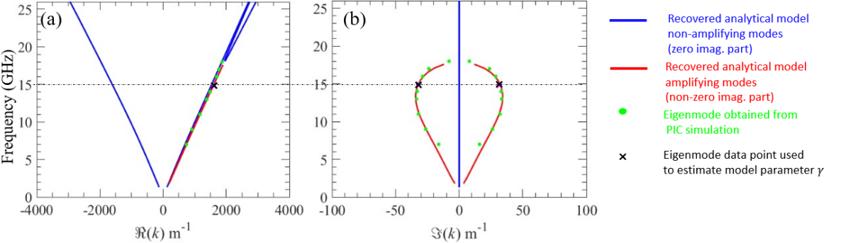
Figure 1: Complex-valued wavenumbers of the hot eigenmodes in the interactive electron beam-EM mode in the helical SWS in Fig. 2(a). (a-b) Real-imaginary parts of the recovered dispersion by estimating the adjusted analytical model ($\gamma$) parameter using PIC simulations data (the black cross data point) and the frequency dependence of cold wavenumber $w(\omega)$ and $\gamma(\omega)$, directly obtained from the cold CST eigenmode solver in Fig. 10. A good agreement is observed in the real part in (a) as well as the imaginary part in (b) between the recovered adjusted analytical model and PIC simulations data (the green dots).

The above mentioned spectral information allows in turn to reconstruct the analytical model parameters and its frequency dependence. From the analytical model we obtain the complex-valued ($\omega$-$k$) dispersion relation of the hot eigenmodes in the TWT (i.e., in the beam-EM interactive system). This dispersion relation is compared side by side with data obtained from PIC simulations at various frequencies. As one can see from Fig. 1, the dispersion relation based on the recovered analytical model is in excellent agreement with results from three dimensional PIC multi-frequency simulations for the helical-based TWT shown in Fig. 2. The dispersion relation and the frequency dependence of the imaginary part of the complex-valued wave numbers provide valuable information on the TWT operation. For instance, the amplification region refers to the range of the frequencies where $\Im(k)>0$ and the TWT gain is directly related to $\Im(k)$. The constructed analytical model with frequency dependence parameters accomplishes our primary goal to model TWT operations for a wide range of frequencies accurately as verified by the comparison with PIC simulations. Taking into account the complexity of TWT operation and its simulation, the simplicity of the analytical model and its excellent agreement with PIC simulations is rather remarkable.

The remainder of this article is organized as follows. Section II presents a brief review of the analytical model used to describe the system and associated model parameters. Section III presents the proposed approach to obtain hot eigenmodes of interest in a TWT using a single PIC simulation (at one frequency). Section IV demonstrates the connection between the analytical model and actual electron beam device based on eigenmode and dispersion relations analysis. Conclusions are presented in Section V.

II Mathematical Formulation

We briefly review the analytical model of TWTs used in this paper. An effective mathematical model for a TWT was introduced by Pierce [11, 4]. This model can be considered as the simplest one that accounts for EM wave amplification and the electron beam energy conversion into microwave radiation in the TWT [16, 9, 2]. The Pierce model, also known as the 4-wave theory of a TWT, is one-dimensional linear theory in which the SWS is represented by a lossless transmission line (TL), assumed to be homogeneous, that is, with uniformly distributed capacitance and inductance [3, 4, 9]. An approximation to the 4-wave theory is the 3-wave small-signal theory which laid the foundation for TWT design [4].

The analytical model used in this paper is a generalization of the Pierce theory, based on the Lagrangian field framework presented in Refs. [5, 6], that, in particular, takes into account the space charge effects. The Lagrangian field theory in [5, 6], allows also to model more complex SWSs than the simple one represented by Pierce by involving more than one SWS mode and multi-stream beam. We provide below a concise summary of the simplest case of a single-stream electron beam coupled to a single TL representing the primary eigenmode of the SWS.

The state of the TWT system is described by variables $Q(t,z)=\int_{t_{0}}^{t}I(t^{\prime},z)dt^{\prime}$ and $q(t,z)=\int_{t_{0}}^{t}i(t^{\prime},z)dt^{\prime}$ where $I$ and $i$ are respectively the TL line and the electron beam currents, $t_{0}$ is the initial time. Variables $Q$ and $q$ represent the amount of charge that has traversed the cross-section of the transmission line and the electron beam, respectively, at point $z$, from time $t_{0}$ to time $t$. Then, following [6], we introduce the TWT-system Lagrangian $\mathcal{L}_{TB}$ as

$$\mathcal{L}_{TB}=\mathcal{L}_{Tb}+\mathcal{L}_{B},$$ (1)

where the Lagrangian components $\mathcal{L}_{Tb}$ and $\mathcal{L}_{B}$ are associated with the SWS and the electron beam respectively and are defined as follows

$$\mathcal{L}_{Tb}=\frac{L}{2}\left(\partial_{t}Q\right)^{2}-\frac{1}{2C}\left(\partial_{z}Q+b\partial_{z}q\right)^{2},$$ (2)

$$\mathcal{L}_{B}=\frac{v_{0}^{2}\partial_{z}q\partial_{t}q}{2\beta}-\frac{2\pi}{\sigma_{B}}q^{2}.$$ (3)

Here, $\sigma_{B}$ is the cross-section of electron beam and $v_{0}$ is the electron beam stream velocity. The symbols $\partial_{t},\partial_{z}$ represents the partial derivative with respect to time $t$ and space $z$, respectively. The parameters $L$ and $C$ are , respectively, the distributed inductance and capacitance associated with the single TL. The term $b$ in 2 describes how the electron beam couples to the TL. The representation of the coupling between an electron beam and a SWS goes back to Ramo [17]. The debunching effects are considered by the term $-2\pi q^{2}/\sigma_{B}$ in equation 3. The parameter $\beta$ is the electron beam stream intensity and it equals $\sigma_{B}R_{sc}^{2}\omega_{p}^{2}/(4\pi)$, where $\omega_{p},R_{sc}$ are the corresponding plasma frequency and plasma frequency reduction factor, respectively. The Euler-Lagrange equations associated with the Lagrangian are the following system of second-order differential equations:

$$L\partial_{t}^{2}Q-\frac{1}{C}\left(\partial_{z}^{2}Q+b\partial_{z}^{2}q\right)=0,$$ (4)

$$\frac{1}{\beta}\left(\partial_{t}+v_{0}\partial_{z}\right){}^{2}q+\frac{4\pi}{\sigma_{B}}q-\frac{b}{C}\left(\partial_{z}^{2}Q+b\partial_{z}^{2}q\right)=0.$$ (5)

Since the beam parameters are assumed constant in space, we can make use of the dispersion relation to study the eigenmodes. With that in mind, we consider solutions of the form $q(z,t),\>Q(z,t)\propto e^{j(\omega t-kz)}$. In the case of spatially uniform (homogeneous) TL, the Fourier transform, in time $t$ and space variable $z$, of equations 4, 5 yields

$$\left(\frac{k^{2}}{C}-\omega^{2}L\right)\hat{Q}+\frac{k^{2}}{C}b\hat{q}=0,$$ (6)

$$\left[\frac{4\pi}{\sigma_{B}}-\frac{1}{\beta}\left(\omega-v_{0}k\right)^{2}\right]\hat{q}+\frac{k^{2}}{C}\left(b^{2}\hat{q}+b\hat{Q}\right)=0,$$ (7)

where $\omega$ and $k$ are respectively the frequency and the wavenumber, and $\hat{Q}=\hat{Q}(\omega,k)$ and $\hat{q}=\hat{q}(\omega,k)$ are the Fourier transforms of the system variables $Q(t,z)$ and $q(t,z)$, respectively. The above system of linear equations 6, 7 is of special interest to us as for it encodes important information on the TWT system including its dispersion relations and the structure of the eigenmodes. For every fixed $\omega$, the linear system 6, 7 are viewed as a kind of eigenvalue problem, which is not the standard eigenvalue problem, where the $k$ is an eigenvalue and the pair $\hat{Q},$$\hat{q}$ forms an eigenvector, see details in [6]. Taking into account the significant role played by the velocities in electron flow interactions, we recast equations 6, 7 by substituting there $k=\omega/u$ where $u$ is the phase velocity of a mode in the interactive system. We then solve the system of equations 6, 7 assuming non-trivial (non-zero) solutions, and after elementary transformations we arrive at the following dimensionless form of the dispersion relation

$$D_{s}(u,\omega)=\frac{\left(v_{0}-u\right)^{2}}{u^{2}}+\frac{\gamma}{w^{2}-u^{2}}-\frac{R_{sc}^{2}\omega_{p}^{2}}{\omega^{2}}=0,$$ (8)

where $\gamma=\beta b^{2}/C$ is the system coupling parameter [6] with unit of [velocity]², and $w=1/\sqrt{LC}$ is the cold SWS mode phase velocity (i.e., TL model). The Euler-Lagrange equations 4, 5 and the system of second-order differential equations 6, 7 are written in centimeter–gram–second (CGS) system, whereas the dispersion relation is dimensionless, hence in the following we will use SI units for convenience. In SI units, the parameters $R_{sc}$ and $\omega_{p}$ are given in [18]. The same dispersion relation was also obtained by using a method based on the Pierce model including the space charge effect. The translation between the Lagrangian model parameters used in this framework and the parameters used in Pierce model is listed in the Supplementary Material of [18].

The dispersion equation 8 has three main parameters: (i) the electron stream velocity $v_{0}$ which is chosen to be equal the electron beam particles’ initial velocity; (ii) the SWS TL modal phase velocity $w$, and (iii) the system coupling parameter $\gamma$. Recovering the correct values of these parameters as functions of the angular frequency $\omega$ is not straight forward, and the purpose of this paper is to develop an approach that uses values of these parameters without any recourse to “curve fitting” approximations but rather based on simple cold SWS full-wave simulations and a single (at one frequency) three dimensional PIC simulation as explained next.

Analytical model adjustment

In this subsection, we present a way of improving the agreement between the analytical model previously discussed and real device data by introducing a phenomenological adjustment to the analytical model. The main physics-based modification is the introduction of frequency dependence of parameters $w$ and $\gamma$ 8 that were assumed to be constant in the analytic model. In other words, we adjust the analytical model by assuming that $w=w(\omega)$ and $\gamma=\gamma(\omega)$ in 8, and that yields

$$D_{s}(u,\omega)=\frac{\left(v_{0}-u\right)^{2}}{u^{2}}+\frac{\gamma(\omega)}{w^{2}(\omega)-u^{2}}-\frac{R_{sc}^{2}\omega_{p}^{2}}{\omega^{2}}=0.$$ (9)

The frequency dependence of analytical model parameters ($w$ and $\gamma$) is invoked as an ad-hock to the final characteristics equation in 8. In the following sections, we present an approach to recover the frequency dependent parameters by exploring solution sets of the dispersion equation 8 at one or more frequencies and comparing that to the hot complex-valued eigenmode observations obtained based on PIC simulations.

III TWT hot eigenmodes based on PIC simulations

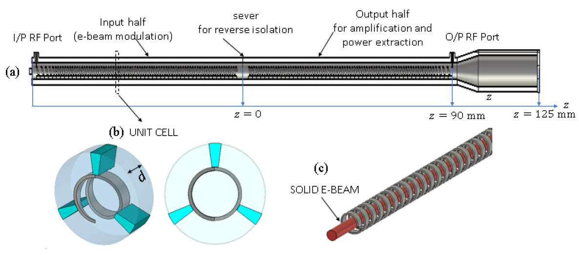
Figure 2: (a) Schematic of a helix-based TWT amplifier. (b) (left) Perspective view and (right) front view of a unit cell of the TWT shown in (a) where the tape helix SWS in the circular waveguide supported by three equally spaced dielectric rods. (c) A solid electron beam flows along the axis of the helical conductor.

Our goal here is to develop an approach of recovering the TWT hot eigenmode information by a thoughtful selection of regimes of TWT operation. The selected regime carries TWT eigenmode information in the most pronounced and undisturbed form. The approach features the estimation of the hot eigenmode information, such as $(\omega,k),$where $\omega$ and $k$ are the angular frequency and the associated complex-valued wave number, respectively, based on one PIC simulation where we extract particles information at one frequency. In general, there is no straightforward way to extract an information about the eigenmodes from commonly performed PIC simulation.

III-A Eigenmode-like operation regime

The eigenmode-like regime of operation is determined by a set of conditions that facilitate the manifestation of the eigenmode frequency and wavenumber dispersion through analyzing observable parameters in PIC simulations. Those conditions include, first, limiting our setup to the region of frequencies where the cold SWS has a single dominant mode. Consequently, the 4-wave theory based on Lagrangian formalism in Sec. II is expected to provide an accurate account for the interaction between the electron beam and the EM wave in the SWS. Second, we would like to suppress backward waves by all means available including introducing a sever. Third, we choose TWT regimes of operation for which nonlinear effects are minimal (i.e., negligible). Suppose now that the above conditions are implemented. Then we carry out PIC simulation assuming that the complex time representation of a chosen observable $s$ (for instance, electric or magnetic field) after reaching the steady state can be represented as follows:

$$s(t,z)=\sum_{i=1}^{4}a_{i}\exp\left\{j\left(\omega t-k_{i}z\right)\right\},$$ (10)

where $\exp\left\{j\left(\omega t-k_{i}z\right)\right\}$ represents the TWT hot eigenmodes, $\omega$ and $k_{i}=k_{i}(\omega)$ are the associated angular frequency and complex-valued wavenumber, respectively. The four modes are the resultant of the interaction between two EM waves in the cold SWS (along $\pm z$) along with two electron beam space-charge waves.

In a simple fully interactive system, four hot eigenmodes form the basis for two regions of operation

1. Amplification region: in this region the four modes are divided into two sets of modes: the first set consists of two exponentially growing and decaying oscillatory modes (amplifying/attenuating, $\Im(k)\neq 0$) such that two modes wavenumbers are complex conjugate to each other (i.e., $k_{1}=k_{2}^{*}$); the second set consists of two oscillatory modes (unamplifying/unattenuating, $\Im\left(k\right)=0$) that vary harmonically in time and are bounded in the entire space by a constant.

2. Non-amplified region: in this region the four modes are oscillatory with real-valued wavenumbers (i.e. $\Im\left(k_{1:4}\right)=0$).

Assumption 1: In the amplification region the amplifying eigenmode is the dominant one. Such that, for a large value of $z$ and after reaching the steady state any observable physical quantity in 10 can readily be approximated as follows:

$$s(t,z)\approx a\exp\left\{j\left(\omega t-k_{i}z\right)\right\},$$ (11)

where subscript $i$ here refers to only the mode with $\Im\left\{k_{i}\right\}>0$, so that the mode $\exp\left\{j\left(\omega t-k_{i}z\right)\right\}$ is amplifying and exponentially growing in space. In view of Assumption 1, the structure hot amplified eigenmode $\exp\left\{j\left(\omega t-k_{i}z\right)\right\}$ is detected by considering the Fourier transformation in spatial variable $z$ of one or more of the observable physical quantities in the PIC simulation. The PIC algorithm uses a three dimensional self-consistent solution of Maxwell’s equations in the time domain in the presence of an electron beam current made of by a finite number of emitted electrons. It also accounts for saturation effects such as electron overtaking. In the following subsection, we show an example of helix-based SWS and the estimation of the amplified eigenmode using observable physical quantities.

III-B Estimation of the amplified eigenmode in helical TWT

We illustrate the efficiency of the approach described in the previous section by considering an example of a C-Band TWT amplifier shown in Fig. 2(a). A helix-based SWS typically consists of a metallic tape-helix inside a metallic waveguide; such SWSs have been used for decades for high power device sources and amplifiers [16, 9, 2]. Figure 2(a) shows an example of helix-based TWT optimized to operate at around 15 GHz, with a total length of about 18 cm comprised of 160 unit cells with period $d$ = 1.04 mm. TWT unit cells are made of a helix metallic tape with an inner radius of 795 $\mu$m, 0.2 mm thickness and 0.51 mm width. The metallic circular waveguide has a radius of 1.06 mm and the three equally spaced dielectric rods support that physically hold the helix are made of BeO dielectric with a relative dielectric constant of 6.5. The input and output radio frequency (RF) signals of the structure are defined as input RF port and output RF port as shown in Fig. 2(a).

We show in Fig. 3 the dispersion relations of the modes in the periodic cold SWS. The cold SWS dispersion diagram indicates that the frequency range of the first quasi-TEM forward mode, which is the reasonable for amplification regime of operation, ends around 25 GHz.

The ($\omega$-$k$) cold dispersion is calculated using the eigenmode solver implemented in CST Suite Studio by DS SIMULIA based on the finite-element method. The eigenmode solver enforces a phase shift across the structure period in the longitudinal direction of propagation and solves for the real-valued eigenfrequencies. The dispersion diagram is constructed by repeating the simulation for different phase shifts.

The cold dispersion diagram shows both forward and backward Floquet-Bloch propagating harmonics in the fundamental Brillouin zone that is here defined from $kd/\pi=0$ to $kd/\pi=2$. The plotted dispersion curves represent only the propagating part of the spectrum and thus, they have a purely real-valued wavenumber $k$. In addition, it is worth emphasizing that the dispersion diagram obtained in Fig. 2(b) is for the cold SWS case (electron beam is absent). However, this cold dispersion is still helpful as a 0th-order approximation to establish synchronization in the fully interactive system (SWS and electron beam). This approximate picture of the interactive system is realized by plotting the “electron beam line” together with the cold dispersion diagram as shown in Fig. 3 in the blue-dashed line. As shown in Fig. 3, the electron beam line intersects with the TEM eigenmode in red around 12 GHz.

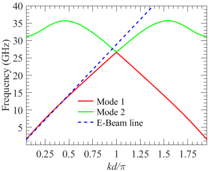
Figure 3: Dispersion diagram of the lowest order Floquet-Bloch eigenmodes of the cold SWS in Fig. 2. An electron beam (e-beam) line with particles’ initial velocity about 0.2 times the speed of light to have a synchronization around the 12 GHz (blue dashed line) is plotted showing that the beam line intersects with the cold dispersion in the forward region.

The hot simulation setup is carried out by CST Studio Suite (PIC solver). The PIC algorithm uses a 3-D self-consistent solution to Maxwell’s equation in the time domain in the presence of an electron beam current made by a finite number of emitted charged particles. It also accounts for saturation effects such as electron overtaking which is responsible for reaching a steady state in an oscillator.

The hot simulation is performed taking into account the eigenmode-like regime considerations by defining particles that are emitted based on the direct current (DC) emission model of the PIC Solver. Such TWT amplifier uses a solid linear electron beam with a radius of 560 $\mu$m. The particles’ initial velocity is 0.2 times the speed of light $c$ (i.e., $v_{0}$ = 0.2$c$) to have a synchronization around 12 GHz in the region where the cold SWS unit cell can be modeled by one cold eigenmode (in each direction) as shown in the cold dispersion and to have a good matching to minimize any rise of the backward (i.e., reflected) modes due to mismatch at the RF ports. The value of the emitted current was set to 10 mA that is less than the threshold current for oscillation, to minimize nonlinear effects. A static axial magnetic field $B_{z}$= 0.64 T is used to ensure a good beam confinement of the solid electron beam traveling in the axial direction. The total number of charged particles used to model the electron beam in the PIC simulation is about 8,901,500 while the whole space in the SWS structure is modeled using 6,640,704 mesh cells.

A PIC simulation is performed to verify the stability of the structure and its immunity to oscillation by running the CST PIC for no RF excitation at the input RF port (red trace), and the signal observed at the output port (blue trace) is shown in Fig. 4(a). It is clear that in the case where there is no RF excitation and since the hot setup configuration, that ensures the stability of the hot structure, the output vanishes after passing the transient time.

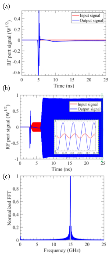
Figure 4: (a) Simulated output RF port signal, for the no RF excitation case, shows no signal after some transient time ~ 10 nS, confirms the stability of the structure, and indicates the time required to reach steady state. (b) Simulated output RF port signal in green shows an amplification occurs to the input RF signal of 10 dBm input and 15 GHz in red, (c) frequency spectrum of the output RF signal shows that the output signal has the same frequency of the signal used to excite the input RF port but with a higher amplitude indicates the amplification operation.

Figure 4(b) shows the output (in blue) and input (in red) RF signals, indicating the amplification level for a single-tune sinusoidal excitation signal of frequency 15 GHz. The frequency spectrum of the output RF signal shown in Fig. 4(c) is obtained by applying Fourier transform to the output RF signal in the time window from 10 nsec to 25 nsec. By utilizing the eigenmode-like regime of operation in the hot setup, one can assume that any observable physical quantity after reaching the steady state resembles the hot amplified eigenmode as in 11.

To estimate the amplified hot eigenmode, we analyze the observable physical quantities obtained in the CST PIC simulations. The PIC solver simulates the complex interaction between the EM wave and electron beam using a large number of charged particles and it follows their trajectories in self-consistent electromagnetic fields computed on a fixed mesh. The physical quantities that represent the EM mode in the interacting SWS are electric and magnetic fields. Also, one can observe physical quantities related to the electron beam such as beam electrons’ energy, momentum, and electron beam charge density.

Figure 5(a) shows a snapshot of the $z$-component of the transient electric field along the SWS after the steady state is reached (on the gap between the SWS and circular waveguide wall). The phasor-domain representation of the $E_{z}(z,t)$ versus $z$ along the SWS is calculated as

$$\mathbf{E}_{z}(z)=\frac{1}{T}\int_{t=t_{0}}^{t=t_{0}+T}E_{z}(z,t)e^{-j\omega t}dt,$$ (12)

where $t_{0}$ is any time instant after steady state is observed, and $T=2\pi/\omega$. The phasor $\mathbf{E}_{z}(z)$ is depicted in Fig. 5(b, c) in terms of magnitude and phase, respectively.

It is apparent that there is more than one spatial frequency component in the field data shown in Fig. 5. Those spatial frequency components are obtained by taking the Fourier transform of the $\mathbf{E}_{z}(z)$. We report the normalized spatial spectrum in Fig. 6 showing different spatial frequency components where the fundamental one that carries most of the energy is $k=1580\,\textrm{m}^{-1}$. Also, it is worth noting that, the plotted normalized spatial spectrum in Fig. 6 invokes other modes from PIC simulations that are not part of the analytical model eigenmodes solution. Those other modes are related to the Floquet-Bloch modes associated with the periodic SWS such as $k_{n}=k_{0}+2\pi n/d$ where $n$ is an integer number representing the order of harmonics. For the particular illustrative example shown here, we report that $k_{0}=1580\,\textrm{m}^{-1}$ and $2\pi/d=6041.5\,\textrm{m}^{-1}$ accordingly the corresponding $-1$ Floquet-Bloch harmonic $k_{-1}=-4461.5\,\textrm{m}^{-1}$, similarly for the negative fundamental $k_{0}=-1580\,\textrm{m}^{-1}$ the corresponding $+1$ Floquet-Bloch harmonic is $k_{1}=4461.5\,\textrm{m}^{-1}.$

Similarly, we apply the same procedure to a physical quantity related to the electron beam such as electrons’ energy. In reality, the energy of the electrons in the beam does not have a single value at each $z$ point. The energy usually depends on each electron transverse location, hence it is convenient to deal with the average of all electrons’ energies at each transverse $z$-dependent cross section such that at each point $z$ the electrons’ energy is represented by a single value representing their average, as was done for the beam electrons’ speed in [15, Eqn. 6].

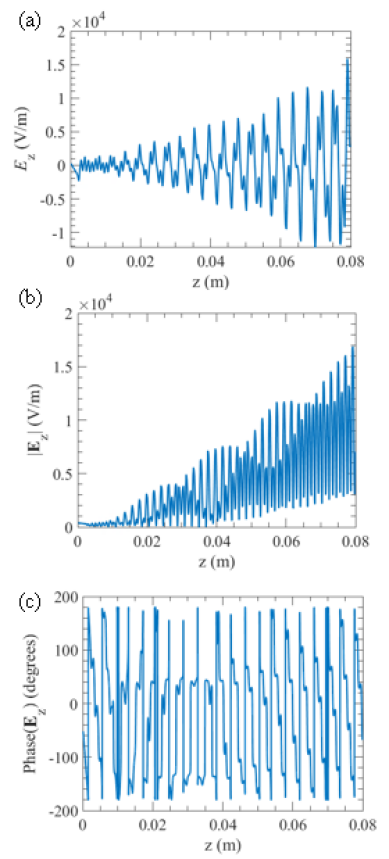
Figure 5: (a) A snapshot in time at $t=10$ nS of the transient $\mathbf{E}_{z}$-field just outside the helix along the SWS after reaching steady state time. (b, c) Phasor $\mathbf{E}_{z}$-field in terms of amplitude and phase along the SWS.

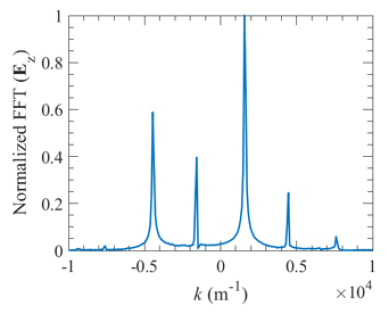
Figure 6: Spatial frequency components of longitudinal electric field associated to the hot structure obtained by performing FFT of phasor $\mathbf{E}_{z}(z)$ shown in Fig. 5 in the space window from $z=0$ to $z=0.08$ m.

Figure 7(a) shows a snapshot of the average kinetic energy of the beam’s electrons along the SWS after steady state is reached. The phasor-domain representation of small-signal kinetic energy (i.e., by subtracting the time-averaged kinetic energy) of the electron beam “AC-Energy” is calculated similarly to the $E_{z}$ in 12. The phasor small-signal kinetic energy is depicted in Fig. 7(b, c) in terms of magnitude and phase, respectively.

It is apparent that there is only one spatial frequency component in the electron beam data shown in Fig. 7, which is contrary to the electric field spectrum that involves Floquet-Bloch modes due to the periodicity nature of the SWS. We report the normalized spatial spectrum of phasor small-signal kinetic energy in Fig. 8 where its spatial frequency is $k=1595\,\textrm{m}^{-1}$. This spatial frequency component is directly related to the eigenmode that is harvesting energy from the electron beam.

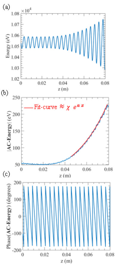
Figure 7: (a) A snapshot in time at $t$ = 10 nS of the average beam electrons’ energy along the SWS after reaching steady state time. (b, c) Complex-valued AC part of the phasor beam electrons’ energy in terms of amplitude and phase. Red line in (b) represents the exponential curve $\chi e^{\alpha z}$ with $\alpha=31.6\,\textrm{m}^{-1}$ and $\chi=19.7\,\textrm{eV}$ which fits well to the magnitude growth of the AC part of beam electrons’ energy.

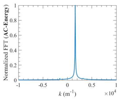
Figure 8: Spatial frequency components of electron beam energy associated to the TWT obtained by performing FFT of phasor AC-Energy shown in Fig. 7 in the space window from $z=0$ to $z=0.08$ m.

By analyzing the spatial frequency spectrum of such physical observables at a certain frequency one can estimate the dominant amplified eigenmode complex-valued wavenumber and the corresponding complex-conjugate attenuated eigenmode. For the helical TWT understudy and from the spatial frequency spectrum in Fig. 8 and the amplitude growth rate reported in Fig. 7(b) the estimated eigenmodes are $(\omega,k)\sim(15\textrm{GHz},1595\pm j31.6\textrm{m}^{-1}$).

IV Connection between the analytical model and actual electron beam device

TWT observables, like EM fields and beam electrons’ energy, are used to determine the analytical model parameters ($\gamma$, $w$) through full-wave simulations either for the model with constants parameters or the adjusted model with dispersive model parameters. As to their qualification to be TWT observables, we notice that by their very definition these observables are some of the parameters associated to the amplified eigenmode in the fully interactive system, since the amplified eigenmode is the dominating the others for z-locations away from the input port. The wavenumber-frequency dispersion describing the eigenmodes in the TWT is determined by running multiple PIC simulations at different frequencies and then determining hot amplified eigenmode ($\omega,$ $k_{PIC}$) at each. Those eigenmodes can be observed through a series of PIC simulations each where the structure is excited by a single tone RF signal. Notice also that TWT observables give knowledge about the complex-valued wavenumbers $k$ for certain frequency $\omega$ at which the TWT dispersion relations as well the TWT characteristic function $D_{s}(\omega,\,k)$ solutions attain instabilities (i.e. convective instability referring to growing and decaying waves with space) as discussed in Sec. II.

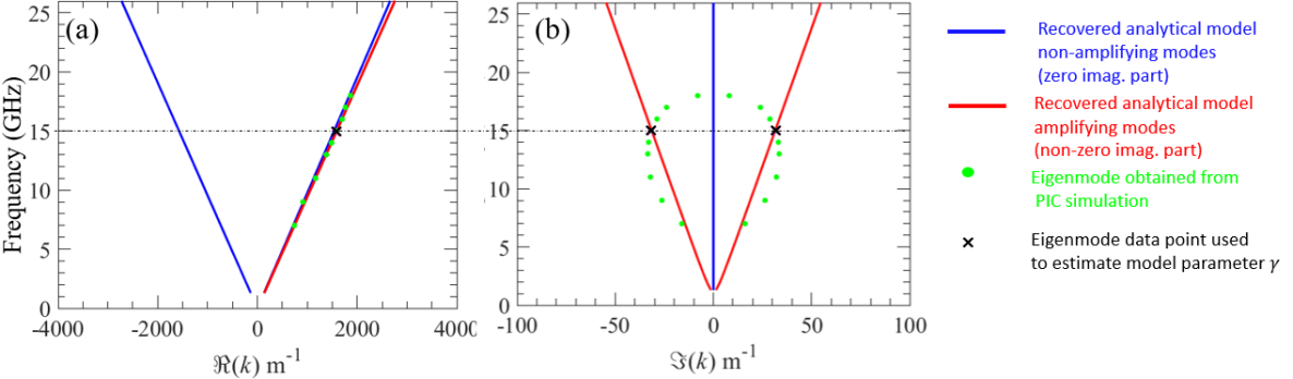
Figure 9: Recovered dispersion diagram, assuming the model parameters are frequency independent. Complex-valued wavenumbers of the eigenmodes in the interactive electron beam-EM mode in the helical SWS in Fig. 2(a). (a) Real part of the recovered dispersion by estimating analytical model parameters using PIC simulations data, a reasonable agreement is observed in the real part. (b) Imaginary part of the dispersion shows a discrepancy between the recovered model and PIC simulations data. The use of a simple analytical model that has only non-dispersive parameters leads to the imaginary parts of the amplified/attenuated modes (red straight lines in (b)) which are not in consistent with PIC simulations data.

To facilitate the computation of analytical model parameter $\gamma$ we would like to optimize $\gamma$ to best fit growing solutions of the dispersion relation 8 $(\omega,\,k_{D_{s}}=\omega/u)$ to the estimated amplified eigenmode through PIC simulations $(\omega,\,k_{PIC})$. This optimization process is applied only at the “estimation frequency”. The estimation frequency can be any frequency in the vicinity of the synchronization frequency, within the amplification region. A common way to deal with this kind of problem is to look for analytical parameter $\gamma$ that minimizes error between the analytical model $k_{D_{s}}$ and PIC $k_{PIC}$ data for the estimated frequency $\omega$, by defining the following error function:

$$\mathscr{E}=c_{1}\left|\Re\left(k_{D_{s}}-k_{PIC}\right)\right|{}^{2}+\left|\Im\left(k_{D_{s}}-k_{PIC}\right)\right|{}^{2},$$ (13)

where $c_{1}$ is a weighting coefficient to equate the importance of the real and imaginary parts of the wavenumbers since there are orders of magnitude difference between the real and imaginary parts of $k$. In particular, given the aforementioned estimated eigenmode $(\omega,\,k_{PIC})\sim(15\textrm{GHz},\,1595+j31.6\textrm{m}^{-1}$), the constant $c_{1}$ was set to be equal to the ratio between the imaginary and real parts of $k$, i.e., $c_{1}=$31.6/1595. Then the expression of the error function is minimized numerically by optimizing the analytical parameter $\gamma$.

For the particular illustrative example shown here, the parameters are as follows: $v_{0}=w=0.2c$ are the parameters (electrons velocity and cold EM mode phase velocity) that are established initially for the synchronized regime of operation, whereas the optimized analytical parameter is $\gamma=8.651\times 10^{10}\,\textrm{$\textrm{m}^{2}$}/\textrm{s}^{2},$ where $\gamma$ is optimized based on the PIC data at 15 GHz (e.g., a frequency at or near the synchronization point) by minimizing the error function. In Fig. 9, blue and red solid lines show the recovered dispersion for the optimized analytical parameters. For the sake of comparison and validation of the proposed model, we also perform PIC simulations at different frequencies and follow to the approach described in Sec. III to estimate the hot amplified eigenmode for each frequency. The PIC-based hot amplified eigenmodes are depicted in Fig. 9 in green circle dots. A reasonable agreement is observed between the dispersion obtained by the proposed model and actual data from PIC simulations, for the real part of the dispersion in Fig. 9(a). Whereas, the imaginary part of the dispersion shown in Fig. 9(b) shows a discrepancy except at 15 GHz “black cross symbol” which is the CST PIC data point used to optimize $\gamma$. The discrepancy at the other frequency points can be explained as the result of using a simple analytical model that has only non-dispersive parameters (i.e., $\gamma,v_{0},\textrm{and }w$ defined as frequency-independent which is not practically true). The model is easily improved as described in the following subsection, where the frequency variation of two fundamental cold SWS parameters is accounted for.

Adjusted analytical model

In this subsection, we show an improved matching between the analytical model and PIC results attributed to the adjusted analytical model. The adjustment is the replacement of constants $w$ and $\gamma$ with the corresponding frequency dependent functions $w(\omega)$ and $\gamma(\omega)$. The phase velocity frequency dependence $w(\omega)$ is obtained from the cold full-wave simulation by analyzing wave propagation in the SWS in the absence of the electron beam to get the $w(\omega)$ to be used in our analytical model recovery method. The frequency dependence of $\gamma$ is also obtained from the cold simulation and relation $\gamma(\omega)=B/C(\omega)$ where $C(\omega)$ is the frequency-dependent equivalent per-unit-length capacitance of the TL model of the SWS as discussed in [18], and $B$ is an adjustment constant which is evaluated by minimizing the error function in (13). We simulated the helix-based cold SWS by using the finite element-based eigenmode solver implemented in CST Suite Studio and extracted the (i) cold-circuit EM phase velocity $w(\omega)$ normalized to the speed of light $c$ as shown in Fig. 10, and (ii) the characteristic wave impedance $Z_{c}(\omega)$ of the mode under interest (i.e., mode 1 “red trace” in the cold dispersion shown in Fig. 3). By using $w(\omega)$ and $Z_{c}(\omega)$, one obtains the equivalent frequency-dependent distributed inductance $L(\omega)=Z_{c}(\omega)/w(\omega)$ and capacitance $C(\omega)=1/\left[Z_{c}(\omega)w(\omega)\right]$.

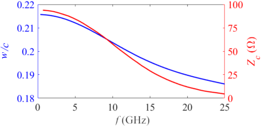
Figure 10: (Blue) Normalized phase velocity and (Red) characteristic impedance of the first forward mode of the SWS shown in Fig. 2(a) obtained from cold full-wave simulations in the absence of the electron beam, using the finite element method-based eigenmode solver.

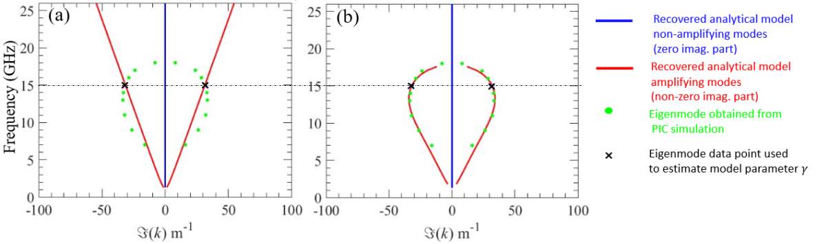
Figure 11: Comparison between imaginary parts of the wavenumbers of the hot eigenmodes for the helical SWS shown in Fig. 2(a) for two analytical models: (a) frequency-independent parameters ($\gamma$, $w$) analytical model in 8, (b) frequency-dependent parameters ($\gamma(\omega)$, $w(\omega)$) adjusted analytical model in 9. The use of a simple analytical model that has dispersive parameters leads to the imaginary part of the amplified/attenuated modes (red lines in (b)) to be consistent with PIC simulations data, contrary to what was observed when using the non-dispersive model (red lines in (a)).

Figure 1 depicts the recovered complex-valued wavenumbers dispersion of the hot modes with an electron beam whose electrons have an initial velocity of $v_{0}=0.2c$ using the adjusted analytical parameters as follows: the frequency dependent phase velocity of the EM cold mode $w(\omega)$ is obtained from full-wave cold simulations, and the optimized adjustment parameter $B=71.28\,\textrm{F}\cdot\textrm{m}/\textrm{s}^{2}.$ Note that, $B$ is evaluated at only the “estimation frequency” (by minimizing the error function in 13 at the estimation frequency of 15 GHz) and then the frequency dependence of $\gamma(\omega)$ is found from $\gamma(\omega)=B/C(\omega)$, where the TL distributed capacitance $C(\omega)$ is obtained from full-wave cold simulations. The dispersion obtained by the model is compared with the hot eigenmode obtained directly from the PIC simulations, plotted by green circular dots, showing a significant improvement in the agreement between the recovered dispersion and actual data from PIC simulations when compared to the results of the model without frequency dependent parameters. To facilitate the comparison,

in Figure 11, we plot side by side the imaginary part of the recovered dispersion using the analytical model without frequency dependent parameters in Fig. 11(a), and the phenomenological adjusted one using frequency dispersion in Fig. 11(b) to emphasize the significant improvement of the model in matching real data obtained from CST PIC simulations.

V Summary

An adjusted analytical model for TWTs is proposed that gives accurate predictions of the wavenumber-frequency dispersion relation and the frequency dependent gain/amplification. The approach utilizes primary frequency-dependent parameters of the cold SWS (modal wave velocity and equivalent TL capacitance) recovered by using a standard procedure, and only one PIC simulation of the TWT, at one frequency, to find the adjustment parameter B without curve fitting. The proposed adjusted analytic model was tested against results obtained directly from PIC simulation for a helical-based TWT operating in the GHz range and showed an excellent agreement. Our extensive preliminary studies suggest that the proposed approach can be applied to different kinds of TWTs including those based on the serpentine SWS. The method can also be extended to retrieve other important TWT parameters like the plasma frequency reduction factor.

VI Acknowledgments

This material is based upon work supported by the Air Force Office of Scientific Research award number FA9550-19-1- 0103. The authors are thankful to DS SIMULIA for providing CST Studio Suite that was instrumental in this study.

References

- [1] J. Benford, J. A. Swegle, and E. Schamiloglu, High power microwaves. Boca Raton, FL, USA, CRC Press, 2015.
- [2] A. S. Gilmour, Klystrons, traveling wave tubes, magnetrons, crossed-field amplifiers, and gyrotrons. Norwood, MA, USA: Artech House, 2011.
- [3] J. R. Pierce, “Theory of the beam-type traveling-wave tube,” Proceedings of the IRE, vol. 35, no. 2, pp. 111–123, 1947.
- [4] ——, Travelling-wave tubes. New York, NY, USA: Van Nostrand, 1950.
- [5] A. Figotin and G. Reyes, “Multi-transmission-line-beam interactive system,” Journal of Mathematical Physics, vol. 54, no. 11, p. 111901, 2013.
- [6] A. Figotin, An Analytic Theory of Multi-stream Electron Beams in Traveling Wave Tubes. World Scientific, 2020.
- [7] J. G. Wohlbier, J. H. Booske, and I. Dobson, “The multifrequency spectral eulerian (muse) model of a traveling wave tube,” IEEE Transactions on Plasma Science, vol. 30, no. 3, pp. 1063–1075, 2002.
- [8] M. C. Converse, J. H. Booske, and S. C. Hagness, “Impulse amplification in a traveling-wave tube-i: Simulation and experimental validation,” IEEE Transactions on Plasma Science, vol. 32, no. 3, pp. 1040–1048, 2004.
- [9] S. E. Tsimring, Electron beams and microwave vacuum electronics. Hoboken, NJ, USA: John Wiley & Sons, 2006, vol. 191.
- [10] P. A. Sturrock, “Kinematics of growing waves,” Physical Review, vol. 112, no. 5, p. 1488, 1958.
- [11] J. R. Pierce, “Circuits for traveling-wave tubes,” Proceedings of the IRE, vol. 37, no. 5, pp. 510–515, 1949.
- [12] Y. Lau and D. Chernin, “A review of the ac space-charge effect in electron–circuit interactions,” Physics of Fluids B: Plasma Physics, vol. 4, no. 11, pp. 3473–3497, 1992.
- [13] D. H. Simon, P. Wong, D. Chernin, Y. Lau, B. Hoff, P. Zhang, C. Dong, and R. M. Gilgenbach, “On the evaluation of pierce parameters c and q in a traveling wave tube,” Physics of Plasmas, vol. 24, no. 3, p. 033114, 2017.
- [14] V. A. Tamma and F. Capolino, “Extension of the Pierce Model to Multiple Transmission Lines Interacting With an Electron Beam,” IEEE Transactions on Plasma Science, vol. 42, no. 4, pp. 899–910, Apr. 2014.
- [15] T. Mealy and F. Capolino, “Traveling wave tube eigenmode solver for interacting hot slow wave structure based on particle-in-cell simulations,” arXiv preprint arXiv:2010.07530, 2020.
- [16] A. S. Gilmour, Principles of traveling wave tubes. Norwood, MA, USA: Artech House, 1994.
- [17] S. Ramo, “Currents Induced by Electron Motion,” Proceedings of the IRE, vol. 27, no. 9, pp. 584–585, Sep. 1939.
- [18] K. Rouhi, R. Marosi, T. Mealy, A. F. Abdelshafy, A. Figotin, and F. Capolino, “Exceptional degeneracies in traveling wave tubes with dispersive slow-wave structure including space-charge effect,” Applied Physics Letters, vol. 118, no. 26, p. 263506, 2021.