Spatial modeling of day-within-year temperature time series: an examination of daily maximum temperatures in Aragón, Spain

Abstract

Acknowledging a considerable literature on modeling daily temperature data, we propose a multi-level spatio-temporal model which introduces several innovations in order to explain the daily maximum temperature in the summer period over $60$ years in a region containing Aragón, Spain. The model operates over continuous space but adopts two discrete temporal scales, year and day within year. It captures temporal dependence through autoregression on days within year and also on years. Spatial dependence is captured through spatial process modeling of intercepts, slope coefficients, variances, and autocorrelations. The model is expressed in a form which separates fixed effects from random effects and also separates space, years, and days for each type of effect. Motivated by exploratory data analysis, fixed effects to capture the influence of elevation, seasonality and a linear trend are employed. Pure errors are introduced for years, for locations within years, and for locations at days within years. The performance of the model is checked using a leave-one-out cross-validation. Applications of the model are presented including prediction of the daily temperature series at unobserved or partially observed sites and inference to investigate climate change comparison.

Keywords: Autoregression; Gaussian process; hierarchical model; long-term trend; Markov chain Monte Carlo; spatially varying coefficients

1 Introduction

Evidence of global warming in the climate system is strong and many of the observed changes since the 1950s are unprecedented, with an estimated anthropogenic increase of 0.2^∘C per decade due to past and ongoing emissions (IPCC, 2013, 2018). Climate change raises significant concerns as it may result in health problems and death, degradation of flora and fauna biodiversity, reductions in crop production and increase of pests, etc. In this framework, the analysis of daily maximum temperatures and their long-term trends over time is particularly important due to the strong potential impact on public health (Roldán et al., 2016; Rossati, 2017; Watts et al., 2015), agriculture (Hatfield et al., 2011; Schlenker and Roberts, 2009), and economy (Diffenbaugh and Burke, 2019).

We propose a new multi-level spatio-temporal model to explain the daily maximum temperature in the summer period, in an area containing the Comunidad Autónoma de Aragón in the northeast of Spain. The region includes part of the Ebro Valley in the center, with mountainous areas in the south (Iberian System) and north (Pyrenees). The valley is an extensively irrigated production area with garden crops, fruits and vegetables, as well as rainfed agriculture with cereals, almonds, wine and oil. In the mountainous areas there are some protected natural spaces with extensive forests and a high diversity of landscapes. It is an area of great biodiversity with important water resources for the region. Despite its relatively small size, spatio-temporal modeling of the temperatures in this region is a challenge due to the heterogeneous orography and the climatic variability.

The spatio-temporal model seeks to characterize spatial patterns and detect trends over time in the daily maximum temperature during the summer period. It is specified over continuous space but adopts two discrete units of time, years and days within years. This allows us to model the time evolution of daily maximum temperatures during the summer, omitting the cooler months that are not of interest here. The model introduces temporal dependence using autoregression terms for days within years and also for years. The model separates fixed and random effects in the mean. Fixed effects capture the global mean, the seasonal component across days, the average long-term trend across years, and the influence of elevation. Random effects are employed for the spatial dependence in the intercepts, the slope coefficients, the autoregression coefficients, and the variances of the responses. The two temporal scales allow us to separate space, years, and days within years for each type of effect. Three pure error processes are adopted, one for locations at days within years, one for locations within years, and one for years. The full specification is motivated by exploratory analyses. Altogether, the model provides a better understanding of the temporal evolution of temperatures for the entirety of the region along with the spatial uncertainty linked to those features.

The model is specified in a hierarchical Bayesian framework and estimated using a Markov chain Monte Carlo (MCMC) algorithm. In this framework, posterior predictive distributions for the features of daily maximum temperatures (trends, persistence, mean, variance, etc.) can be readily obtained. In particular, we can obtain posterior predictive samples of the spatial processes and the daily maximum temperature series at unobserved sites. Prediction at unobserved sites is particularly important in Aragón since this region is sparsely monitored due to rural depopulation; there is a lack of observed series in many areas of interest. The model can also be used to impute periods of missing observations in a series.

Space-time modeling of environmental series has received substantial attention in the literature. Sahu et al. (2006) proposed a random effects model for fine particulate matter concentrations in the midwestern United States. Sahu et al. (2007) proposed a space-time hierarchical model for daily 8-hour maximum ozone levels in the state of Ohio. This model includes an autoregressive part for the residuals of the fixed effects, a global annual intercept and a spatially correlated error term. Lemos et al. (2007) modeled monthly water temperature data in a Central California Estuary. They used a Bayesian approach to separate the seasonal cycle, short-term fluctuations, and long-term trends by means of local mixtures of two patterns. With regard to temperature models, Craigmile and Guttorp (2011) built space‐time hierarchical Bayesian models using daily mean temperatures in Central Sweden that emphasize modeling trend through a wavelet specification, as well as seasonality, and error that may exhibit space‐time long‐range dependence. Verdin et al. (2015) modeled maximum and minimum temperature to develop a weather generator using spatial Gaussian processes (GPs), where both temperature models are autoregressive with spatially varying model coefficients and spatial correlation. Li et al. (2020) proposed a three step space-time regression-kriging model for monthly average temperature data. With such data, they first remove seasonality, then they regress the revised data on environmental predictors, and finally they take the resulting residuals and administer spatio-temporal variogram modeling. By contrast, models for daily temperatures take a different approach, seeking to explicitly express short-term persistence of temperature. They employ autoregressive terms, e.g., the one-point model by Mohammadi et al. (2021). A modeling approach very different from our mean specification considers extremes in the daily temperature series and leads to extreme value modeling under the block maxima framework or peaks-over-threshold framework (see, e.g., Reich et al., 2014; Bopp and Shaby, 2017).

The outline of the paper is as follows. An exploratory analysis to motivate the complexity of the model is given in Section 2. Section 3 describes the modeling details, and Section 4 presents a leave-one-out cross-validation (LOOCV) analysis for model comparison as well as some results and applications for the selected model. Section 5 ends the paper with some conclusions and future work. Supplementary Materials accompanying this paper appear online.

2 Data and exploratory analysis

The point-referenced dataset we use contains 18 daily maximum temperature observational series from AEMET (the Spanish Meteorological Office) around the Comunidad Autónoma de Aragón (see Figure 1). The time series include the daily observations from May to September (MJJAS), corresponding to the extended summer period, and span the period from 1956 to 2015. The region of interest is located in the central portion of the Ebro Basin in the northeastern part of Spain and has an area of 53,279 km², wherein the areas above 500 m and 1,000 m are 32,924 km² and 15,195 km² respectively. The maximum elevation is roughly 3,400 m in the Pyrenees, 2,600 m in the Iberian System, and between 200 and 400 m in the Central Valley. Most of the area is characterized by a Mediterranean-Continental dry climate with irregular rainfall and a large temperature range. However, climate differences can be distinguished by elevation and the influence from the Mediterranean Sea in the east as well as the continental conditions of the Iberian Central Plateau in the southwest (AEMET, 2011).

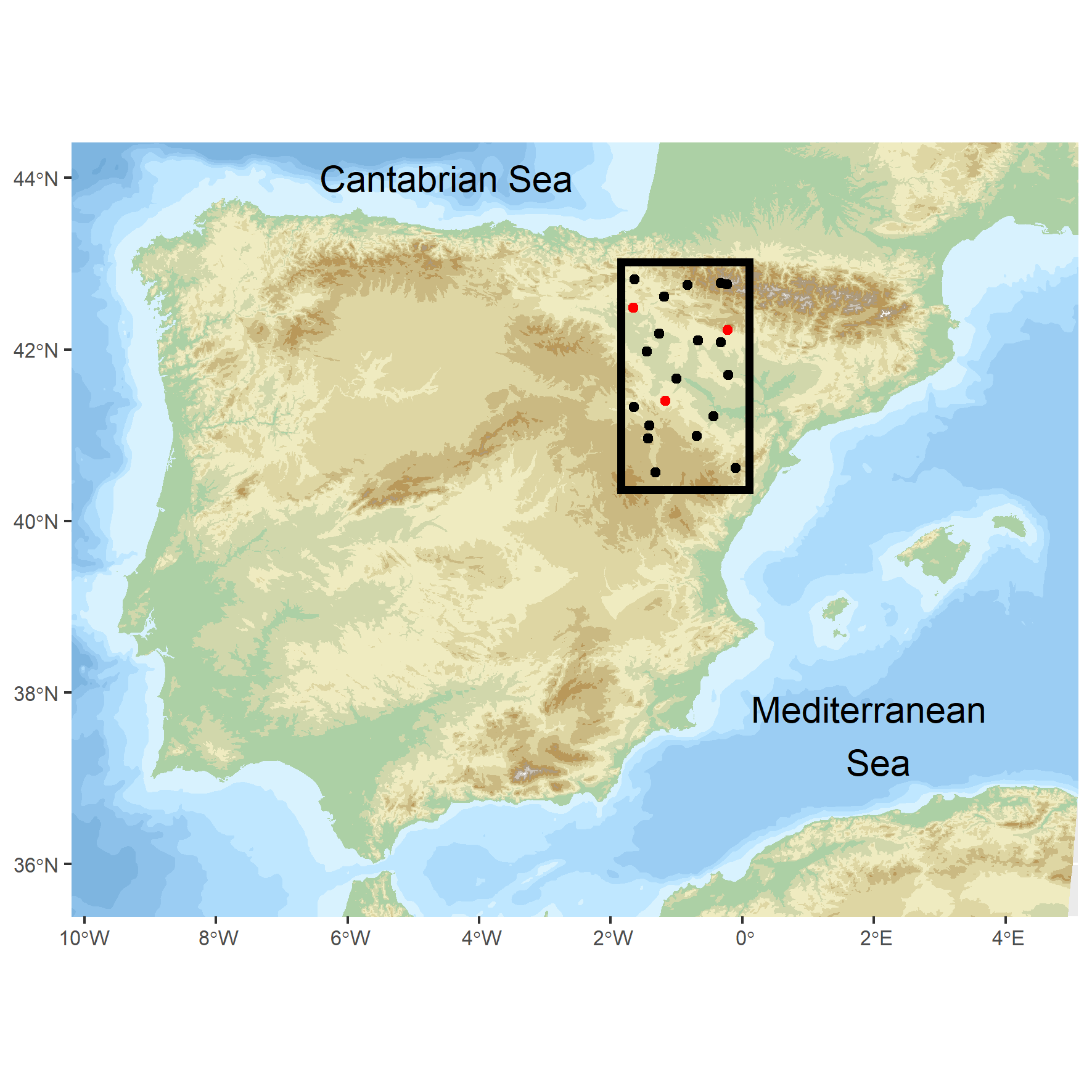
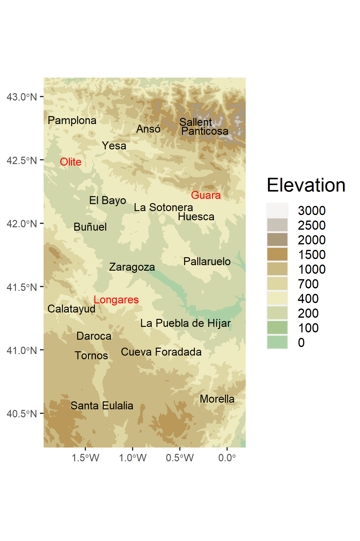
Figure 1: Map locating within the Iberian Peninsula the 18 sites (black) used to fit the model and the 3 unobserved sites (red) where prediction is carried out.

We summarize an extensive exploratory data analysis of the daily maximum temperature series that helps us establish the covariates and spatio-temporal structures that are candidates for inclusion in the model. The top plots in Figure 2 show the variability in temperature characteristics and the influence of elevation on them. The two plots on the left show the mean and the standard deviation of temperature at each site against elevation. The mean temperature shows an approximately linear decreasing relation with elevation, varying from almost $30$ to $18^{\circ}$C. However, there exist other influential factors, e.g., Sallent in the north and Tornos in the south have both an elevation around 1,000 m but a quite lower mean temperature is observed for the latter (see Table S1 in Supplementary Materials).

Figure 2: Top: Mean value, standard deviation, annual time trend, and serial correlation against elevation for the daily maximum temperature series at the 18 sites. Bottom: Mean value and standard deviation of the series in both 30-year periods, 1956–1985 and 1986–2015, and the change between them, expressed as differences for the mean and quotients for the standard deviation.

The bottom plots in Figure 2 summarize the mean and standard deviation from data corresponding to a month in MJJAS for the 18 sites in the periods 1956–1985 and 1986–2015; the summary measures are calculated in 30-year periods following the recommendation of the WMO (2017). The seasonal pattern for all of the series is quite similar, i.e., the maximum mean temperature is observed in July and the minimum in May, with a difference of around $7^{\circ}$C between them. The range of the mean temperatures among sites is around $10^{\circ}$C, so the spatial variability of the mean is a bit higher than the variability at each site within the summer. The mean of the set of standard deviations is slightly higher than $4^{\circ}$C. However, relevant spatial differences are observed with a range of values around $1.5^{\circ}$C. Temporal variability is lower within the summer.

To explore the effect of global warming in the region, the changes between 1956–1985 and 1986–2015 periods, expressed as differences for the means and quotients for the standard deviations, are also shown on the bottom-right plot in Figure 2 and Table S1. The mean temperature in 1986–2015 has increased from 1956–1985 by roughly $1^{\circ}$C, with a slightly smaller increase in the northeastern sites. The increase of the mean temperature is observed in May, June, August and, except for three sites, in July. No relevant change in the seasonal pattern is observed. The spatial variability in the two periods is similar. As for the standard deviations, no evidence of temporal change is observed, with all of the quotients between the two periods being approximately one.

The two plots on the top-right in Figure 2 summarize an exploratory analysis of the behavior of the time series over time. The first shows the slope regressed against year (expressed in ^∘C per decade), fitted by ordinary least squares to the daily maximum temperature series in each site. Clear differences are observed in the 18 fitted trends, suggesting the need to include a spatial random effect to reflect this feature. The variability in the trends does not seem to be related to the elevation. The last plot shows the serial correlation in the temperature series. A strong correlation, higher than 0.72, is observed for all the sites but with spatial differences. The strong autocorrelation is probably caused by a persistent anticyclonic situation that tends to affect the Iberian Peninsula in the summer. Sites with a higher elevation seem to show a slightly higher persistence.

As an additional exploratory analysis, 18 hierarchical temporal models were fitted, one for each of the available sites. These local models, which are summarised in Section S1.1 of the Supplementary Materials, are useful to identify the time structures required for the temperature series and to evaluate the spatial variability of the fitted terms. The results motivate the introduction of spatially varying intercepts, trends, autoregression coefficients, and variances for the spatial variability in the model.

3 The Model

We propose a multi-level (i.e., hierarchical) full mean model for daily maximum temperatures that operates over continuous space and two discrete temporal scales. It captures temporal dependence through autoregression on days within year and on years. It captures spatial dependence through spatial process modeling of intercepts, slope coefficients, variances, and autocorrelations. We detail this model below and then discuss model fitting, prediction under the model, and model comparison.

3.1 Model construction

Let $Y_{t\ell}(\textbf{s})$ denote the daily maximum temperature for day $\ell$, $\ell=2,\ldots,L$ of year $t$, $t=1,\ldots,T$ at location $\textbf{s}\in D$, where $D$ is our study region. Here, for all years, $\ell=1$ corresponds to May 1 and $L=153$ corresponds to September 30. It is convenient to express the full model in a form which separates fixed effects from random effects and also carefully separates space, years, and days for each type of effect. Specifically, we model daily maximum temperature for day $\ell$, year $t$, and location s by

$$Y_{t\ell}(\textbf{s})=\mu_{t\ell}(\textbf{s};\mbox{\boldmath$\theta$}_{f})+\gamma_{t}(\textbf{s})+\rho_{Y}(\textbf{s})\left(Y_{t,\ell-1}(\textbf{s})-(\mu_{t,\ell-1}(\textbf{s};\mbox{\boldmath$\theta$}_{f})+\gamma_{t}(\textbf{s}))\right)+\epsilon_{t\ell}^{(Y)}(\textbf{s}).$$ (1)

Here, $\mu_{t\ell}(\textbf{s};\mbox{\boldmath$\theta$}_{f})$ denotes the fixed effects component and $\gamma_{t}(\textbf{s})$ the random effects component. We specify

$$\mu_{t\ell}(\textbf{s};\mbox{\boldmath$\theta$}_{f})=\beta_{0}+\alpha t+\beta_{1}\text{sin}(2\pi\ell/365)+\beta_{2}\text{cos}(2\pi\ell/365)+\beta_{3}\text{elev}(\textbf{s})$$ (2)

in which $\beta_{0}$ is a global intercept, $\alpha$ is a global linear trend coefficient, the $\sin$ and $\cos$ terms are introduced to provide an annual seasonal component, and $\text{elev}(\textbf{s})$ is the elevation at s. We denote these fixed effect parameters by $\mbox{\boldmath$\theta$}_{f}=(\beta_{0},\alpha,\beta_{1},\beta_{2},\beta_{3})$.

We specify

$$\gamma_{t}(\textbf{s})=\beta_{0}(\textbf{s})+\alpha(\textbf{s})t+\psi_{t}+\eta_{t}(\textbf{s}).$$ (3)

In (3), $\psi_{t}$ follows an AR(1) specification, i.e., $\psi_{t}=\rho_{\psi}\psi_{t-1}+\lambda_{t}$, providing an autoregression in years for annual intercepts. This autoregression could help to capture factors yielding correlation across years such as the influence of variation in solar activity on the earth’s surface temperature or the El Niño Southern Oscillation. However, in Section 3.2, we discover that $\rho_{\psi}$ is not significantly different from $0$. We still need the $\psi$’s in the model to address the fact that some years are warmer or colder than others but we do not need to specify them autoregressively. We denote the variance for this component by $\sigma^{2}_{\lambda}$.

Continuing, $\beta_{0}(\textbf{s})$ is a mean-zero GP with an exponential covariance function having variance parameter $\sigma^{2}_{\beta_{0}}$ and decay parameter $\phi_{\beta_{0}}$, and $\alpha(\textbf{s})$ is a mean-zero GP with an exponential covariance function having variance parameter $\sigma^{2}_{\alpha}$ and decay parameter $\phi_{\alpha}$. Thus, $\beta_{0}(\textbf{s})$ provides local spatial adjustment to the intercept and $\alpha(\textbf{s})$ provides local slope adjustment to the linear trend. Due to the simplicity of linear time trends they are often used in climate studies (IPCC, 2013). Here, they provide an extremely flexible, locally linear baseline specification. Further, we add local space-time varying random effects, $\eta_{t}(\textbf{s})$, to provide adjustment to this baseline. We collect the random effects parameters into $\mbox{\boldmath$\theta$}_{r}=(\rho_{\psi},\sigma^{2}_{\lambda},\sigma^{2}_{\beta_{0}},\phi_{\beta_{0}},\sigma^{2}_{\alpha},\phi_{\alpha})$.

The entire specification is supplied distributionally in the form of a multi-level hierarchical model as

$$\begin{gathered}[Y_{t\ell}(\textbf{s})\mid Y_{t,\ell-1}(\textbf{s}),\mbox{\boldmath$\theta$}_{f},\gamma_{t}(\textbf{s}),\rho_{Y}(\textbf{s}),\sigma^{2}_{\epsilon}(\textbf{s})]\\ [\gamma_{t}(\textbf{s})\mid\beta_{0}(\textbf{s}),\alpha(\textbf{s}),\psi_{t},\sigma^{2}_{\eta}]\\ [\beta_{0}(\textbf{s})|\sigma_{\beta_{0}}^{2},\phi_{\beta_{0}}][\alpha(\textbf{s})|\sigma_{\alpha}^{2},\phi_{\alpha}][\psi_{t}|\psi_{t-1},\rho_{\psi},\sigma_{\lambda}^{2}][Z_{\rho_{Y}}(\textbf{s})|Z_{\rho_{Y}},\sigma^{2}_{\rho_{Y}},\phi_{\rho_{Y}}][Z_{\sigma_{\epsilon}^{2}}(\textbf{s})|Z_{\sigma^{2}_{\epsilon}},\sigma^{2}_{\sigma^{2}_{\epsilon}},\phi_{\sigma^{2}_{\epsilon}}]\\ [\mbox{\boldmath$\theta$}_{f}][\mbox{\boldmath$\theta$}_{r}][\sigma_{\eta}^{2}][Z_{\rho_{Y}}][\sigma_{\rho_{Y}}^{2}][\phi_{\rho_{Y}}][Z_{\sigma_{\epsilon}^{2}}][\sigma_{\sigma_{\epsilon}^{2}}^{2}][\phi_{\sigma_{\epsilon}^{2}}].\end{gathered}$$ (4)

As a result, we have introduced three pure error terms: $\lambda_{t}\stackrel{{\scriptstyle iid}}{{\sim}}N(0,\sigma_{\lambda}^{2})$ at yearly scale, $\eta_{t}(\textbf{s})\stackrel{{\scriptstyle iid}}{{\sim}}N(0,\sigma_{\eta}^{2})$ at sites within years, and $\epsilon^{(Y)}_{t\ell}(\textbf{s})\stackrel{{\scriptstyle ind.}}{{\sim}}N(0,\sigma_{\epsilon}^{2}(\textbf{s}))$ at sites for days within years. Additionally, $\rho_{Y}(\textbf{s})$ and $\sigma_{\epsilon}^{2}(\textbf{s})$ are, respectively, a spatially varying autoregressive term and a spatially varying variance at location s, both of which are assumed constant over days and years. We model $\log\left\{(1+\rho_{Y}(\textbf{s}))/(1-\rho_{Y}(\textbf{s}))\right\}=Z_{\rho_{Y}}(\textbf{s})\sim GP(Z_{\rho_{Y}},C(\cdot;\sigma_{\rho_{Y}}^{2},\phi_{\rho_{Y}}))$, and $\log\{\sigma_{\epsilon}^{2}(\textbf{s})\}=Z_{\sigma_{\epsilon}^{2}}(\textbf{s})\sim GP(Z_{\sigma_{\epsilon}^{2}},C(\cdot;\sigma_{\sigma_{\epsilon}^{2}}^{2},\phi_{\sigma_{\epsilon}^{2}}))$, again with exponential covariance functions. Motivation for adopting spatially varying specifications for these terms arises from exploratory data analysis at the level of the individual sites. That is, suppose we fit the model above but ignore spatial structure and treat the sites as conditionally independent. We show in Section S1.1 of the Supplementary Materials that the assumptions of constant autoregression coefficients and constant variances over the region do not seem justified.

All of the components considered in the full model and their relationships are depicted in the graphical model in Figure 3. This diagram, perhaps, reveals the complexity of the full model more readily than through Equations 1, 2, 3 and 4.

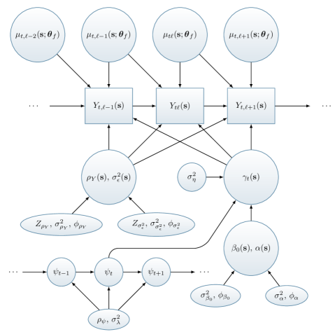
Figure 3: Graphical model for specification in Equations 1, 2, 3 and 4. Rectangular nodes are observed, circular nodes are unobserved.

The reader might wonder if the GPs above are independent. We investigated dependence between the intercept and slope GPs using the following coregionalization (Banerjee et al., 2014, Chapter 9). Suppose $v_{1}(\textbf{s})$ and $v_{2}(\textbf{s})$ are independent GPs with zero mean and unit variance whose exponential covariance functions have decay parameters $\phi_{1}$ and $\phi_{2}$, respectively. In the full model we insert $\beta_{0}(\textbf{s})=a_{11}v_{1}(\textbf{s})$ and $\alpha(\textbf{s})=a_{21}v_{1}(\textbf{s})+a_{22}v_{2}(\textbf{s})$. Here, we let $a_{11}$ and $a_{22}$ each have a half (or folded) Gaussian prior while $a_{21}$ has a regular Gaussian prior. The parameter $a_{21}$ captures the dependence between the two processes. That is, the induced covariance between $\beta_{0}(\textbf{s})$ and $\alpha(\textbf{s})$ is $a_{21}a_{11}$. We care whether $a_{21}$ is significantly different from zero with little interest in exactly what the correlation is. Under the model above, the posterior distribution of $a_{21}$ was centered at zero with wide credible intervals. So, this dependence was not included in the final model for which we present the inference.

Returning to the full model, notice that we have separated the fixed effects according subscripts $t$, $\ell$, and s. As for $\gamma_{t}(\textbf{s})$, we can see that it has a spatially varying intercept, a spatially varying coefficient for drift, and an AR(1) model for years. Also, $\gamma_{t}(\textbf{s})$ has both space and time dependence and, in fact, we can readily calculate $\text{cov}(\gamma_{t}(\textbf{s}),\gamma_{t+h}(\textbf{s}^{\prime}))$. Under independence of the intercept and slope processes, the equilibrium covariance becomes

$$\text{cov}(\gamma_{t}(\textbf{s}),\gamma_{t+h}(\textbf{s}^{\prime}))=C(||\textbf{s}-\textbf{s}^{\prime}||;\sigma_{\beta_{0}}^{2},\phi_{\beta_{0}})+t(t+h)C(||\textbf{s}-\textbf{s}^{\prime}||;\sigma_{\alpha}^{2},\phi_{\alpha})+\frac{\sigma_{\lambda}^{2}}{1-\rho_{\psi}^{2}}\rho_{\psi}^{|h|}.$$ (5)

Finally, special cases of interest include: $\beta_{0}(\textbf{s})=0$ implies a constant intercept over space, $\alpha(\textbf{s})=0$ implies a constant linear drift over space, $\rho_{\psi}=0$ implies no yearly autoregression. These assumptions merely revise the form of $\gamma_{t}(\textbf{s})$. We might consider conditioning on a longer history of maximum temperatures. We experimented with introducing additional lags in the modeling but we found no gain in predictive performance. We could also consider additional fixed effects, e.g., longitude, latitude or distance to coast, or even adding interactions, e.g., $t\times\text{elev}(\textbf{s})$. However, the exploratory analysis did not reveal a relationship between daily temperatures and these fixed effects, so they were not introduced in the full model.

3.2 Model fitting

Model inference is implemented in a Bayesian framework, requiring prior distributions for each of the model parameters. In general, diffuse and, when available, conjugate prior distributions are chosen. Recall that the model adopts a conditional Gaussian distribution for all $Y_{t\ell}(\textbf{s})$’s. Thus it is appropriate to assign each of the coefficient parameters $\beta_{0}$, $\alpha$, $\beta_{1}$, $\beta_{2}$ and $\beta_{3}$, independent and diffuse Gaussian prior distributions with mean $0$ and standard deviation $100$. The variance parameters, $\sigma_{\lambda}^{2}$ and $\sigma_{\eta}^{2}$, are assigned independent Inverse-Gamma$(2,1)$ prior distributions. In preliminary analyses, the autoregresive term between years, $\rho_{\psi}$, was assigned a non-informative Uniform$(-1,1)$ prior distribution. As its posterior distribution was centered at zero with wide credible intervals, we set the parameter at $\rho_{\psi}=0$. For identifiability, the random effect for the first year, $\psi_{1}$, is fixed to zero.

Hyperpriors are assigned to the mean of both $Z_{\rho_{Y}}(\textbf{s})$ and $Z_{\sigma_{\epsilon}^{2}}(\textbf{s})$. That is, $Z_{\rho_{Y}}$ and $Z_{\sigma_{\epsilon}^{2}}$ are given a Gaussian prior distribution with mean $0$ and standard deviation $100$ and $1$, respectively. The variance parameter for each of the four spatial covariance functions, $\sigma_{\beta_{0}}^{2}$, $\sigma_{\alpha}^{2}$, $\sigma_{\rho_{Y}}^{2}$ and $\sigma_{\sigma_{\epsilon}^{2}}^{2}$, is assigned an independent Inverse-Gamma$(2,1)$ prior distribution. Preliminary analyses with a discrete uniform prior distribution for each of the spatial decay parameters indicated that these parameters almost always placed most mass on the smallest decay value. Due to the fact that, with an exponential covariance function, the variance and the decay parameter cannot be individually identified (Zhang, 2004), and the decay parameter is $3/\text{range}$, we set $\phi\equiv\phi_{\beta_{0}}=\phi_{\alpha}=\phi_{\rho_{Y}}=\phi_{\sigma_{\epsilon}^{2}}=3/d_{max}$, where $d_{max}$ is the maximum distance between any pair of spatial locations.

MCMC is used to obtain samples from the joint posterior distribution. The sampling algorithm is a Metropolis-within-Gibbs version. Since we only have $18$ sites, we fit the model without marginalization over the spatial random effects. Also, we introduce $\tilde{\beta}_{0}(\textbf{s})=\beta_{0}+\beta_{0}(\textbf{s})$ and $\tilde{\alpha}(\textbf{s})=\alpha+\alpha(\textbf{s})$ within $\gamma_{t}(\textbf{s})$ for the fitting to enable the benefits of hierarchical centering in the model fitting (Gelfand et al., 1995). Details of the MCMC used for the model fitting are provided in Section S2.1 of the Supplementary Materials. All the covariates have been centered and scaled to have zero mean and standard deviation one to improve the mixing behavior of the algorithm.

3.3 Spatial and spatio-temporal prediction

Under the full model, prediction at location $\textbf{s}_{0}$, day $\ell^{\prime}$, and year $t^{\prime}$ is based on the posterior predictive distribution of $Y_{t^{\prime}\ell^{\prime}}(\textbf{s}_{0})$ arising from the full model. Here, $\textbf{s}_{0}$ may correspond to a fully observed location (held out for validation), a partially observed location (for completion of a record), or a new location in $D$. Our goal is not forecasting, so we restrict ourselves to the observed time period $\ell^{\prime}=2,\ldots,L$ and $t^{\prime}=1,\ldots,T$. Within the Bayesian framework, the posterior predictive distribution for $Y_{t^{\prime}\ell^{\prime}}(\textbf{s}_{0})$ is obtained by integrating over the parameters with respect to the joint posterior distribution. The formal expression for the posterior predictive distribution for $[Y_{t^{\prime}\ell^{\prime}}(\textbf{s}_{0})\mid\textbf{Y}]$, where Y is the observed data, is given in Section S2.2 of the Supplementary Materials. Customarily, the distribution is obtained empirically through posterior samples. That is, with MCMC algorithms, samples of the posterior parameters are used to obtain posterior predictions of observations, so-called composition sampling (see Banerjee et al., 2014, Chapter 6; and Section S2.2 for the details).

3.4 Model evaluation

For model assessment, a LOOCV is carried out to compare the spatial predictive performance of the models. The full model considered includes four spatial GPs. To validate that model as well as the importance of the considered GPs, reduced models incorporating 0, 1, 2, or 3 GPs are fitted. Models are presented explicitly in Section 4.1 where we further clarify that removing particular terms allows explicit interpretation of the resulting reduced models.

Results from Section 4.1 favors the full model and so, results for this model are presented subsequently. However, several of the reduced models yield essentially equivalent global performance, though the fit at some sites is poorer. We attempt to clarify why this might be expected but also show that each set of random effects reveals differences across sites, further encouraging us to retain them in the inference presentation.

For each location in the hold-out set, the entire time series of daily maximum temperatures is withheld during model fitting. Then, for location $\textbf{s}_{i}$, we conduct our model comparison through the following metrics: (i) root mean square error (RMSE), (ii) mean absolute error (MAE), (iii) continuous ranked probability score (CRPS; Gneiting and Raftery, 2007), and (iv) coverage (CVG). By definition,

$$\text{RMSE}_{i} =\sqrt{\frac{1}{T(L-1)}\sum_{t=1}^{T}\sum_{\ell=2}^{L}\left(\hat{Y}_{t\ell}(\textbf{s}_{i})-Y_{t\ell}(\textbf{s}_{i})\right)^{2}},$$

$$\text{MAE}_{i} =\frac{1}{T(L-1)}\sum_{t=1}^{T}\sum_{\ell=2}^{L}\left|\hat{Y}_{t\ell}(\textbf{s}_{i})-Y_{t\ell}(\textbf{s}_{i})\right|,$$

$$\text{CRPS}_{i} =\frac{1}{T(L-1)}\sum_{t=1}^{T}\sum_{\ell=2}^{L}\left(\frac{1}{B}\sum_{b=1}^{B}\left|Y_{t\ell}^{(b)}(\textbf{s}_{i})-Y_{t\ell}(\textbf{s}_{i})\right|-\frac{1}{2B^{2}}\sum_{b_{1}=1}^{B}\sum_{b_{2}=1}^{B}\left|Y_{t\ell}^{(b_{1})}(\textbf{s}_{i})-Y_{t\ell}^{(b_{2})}(\textbf{s}_{i})\right|\right),$$

$$\text{CVG}_{i} =\frac{1}{T(L-1)}\sum_{t=1}^{T}\sum_{\ell=2}^{L}I(L_{t\ell}(\textbf{s}_{i})\leq Y_{t\ell}(\textbf{s}_{i})\leq U_{t\ell}(\textbf{s}_{i})),$$

where $\hat{Y}_{t\ell}(\textbf{s}_{i})=\sum_{b=1}^{B}Y_{t\ell}^{(b)}(\textbf{s}_{i})/B$ with $Y_{t\ell}^{(b)}(\textbf{s}_{i})$ the $b$th posterior predictive replicate of $Y_{t\ell}(\textbf{s}_{i})$, from the left-out location $\textbf{s}_{i}$. Also, $(L_{t\ell}(\textbf{s}_{i}),U_{t\ell}(\textbf{s}_{i}))$ is the $90\%$ predictive interval for $Y_{t\ell}(\textbf{s}_{i})$, i.e., the $5$th and $95$th percentiles of the MCMC samples $Y_{t\ell}^{(b)}(\textbf{s}_{i})$ ($b=1,\ldots,B$), and $I(\cdot)$ is the indicator function. The smaller the RMSE, MAE and CRPS values, the better the model performance. However, the target for CVG is proximity to $0.90$.

4 Results

We summarize, using LOOCV, the comparison of models with differing inclusion of the foregoing spatial GPs. Each model was fitted to the daily maximum temperature series in months MJJAS for the 60 years from 1956 to 2015. Then, we present the results for the fitting of the full model over the study region.

In the MCMC fitting we ran 10 chains, with 200,000 iterations for each chain, to obtain samples from the joint posterior distribution. The first 100,000 samples were discarded as burn-in and the remaining 100,000 samples were thinned to retain 100 samples from each chain for posterior inference. MCMC diagnostics for the full model are shown in Section S2.3 of the Supplementary Materials.

4.1 Validation and model comparison

The full model considered includes four spatial GPs. To compare models and assess the importance of the proposed GPs, simpler models incorporating 0, 1, 2, or 3 GPs are fitted. $M_{p}$ with $p=0,1,\ldots,4$ denotes a model including $p$ spatial processes that are specified in parentheses. For example, $M_{1}(\beta_{0}(\textbf{s}))$ is the model with a single spatial process for the intercept; for simplicity the full model is denoted $M_{4}$.

Using the criteria in Section 3.4 with LOOCV for each of the 18 available locations, Table 1 summarizes the averages across sites for the four metrics. The strongest improvement in predictive performance is obtained by adding a spatially varying intercept process, i.e., $M_{1}(\beta_{0}(\textbf{s}))$. The inclusion of the other GPs does not yield a clear improvement in performance. This is not surprising, since the GP for intercepts explicitly rewards predicting the mean and random realizations well in order to agree with the held-out values. However, the usefulness of the other GPs with regard to effectively capturing autocorrelations and variances at the observed sites will be seen in Section 4.2.

Table 1: Mean value across the 18 sites of the performance metrics for models with different spatial GPs.

	RMSE	MAE	CRPS	CVG
$M_{0}$	4.49	3.64	2.57	0.894
$M_{1}(\beta_{0}(\textbf{s}))$	4.36	3.53	2.49	0.901
$M_{1}(\alpha(\textbf{s}))$	4.49	3.64	2.57	0.894
$M_{1}(\rho_{Y}(\textbf{s}))$	4.49	3.64	2.57	0.895
$M_{1}(\sigma_{\epsilon}(\textbf{s}))$	4.49	3.63	2.56	0.893
$M_{2}(\beta_{0}(\textbf{s}),\sigma_{\epsilon}(\textbf{s}))$	4.36	3.53	2.48	0.901
$M_{3}(\beta_{0}(\textbf{s}),\alpha(\textbf{s}),\sigma_{\epsilon}(\textbf{s}))$	4.36	3.53	2.49	0.899
$M_{3}(\alpha(\textbf{s}),\rho_{Y}(\textbf{s}),\sigma_{\epsilon}(\textbf{s}))$	4.49	3.63	2.56	0.894
$M_{4}$	4.36	3.53	2.48	0.900

Table S4 in the Supplementary Materials provides details, by site, for the metrics in Table 1. The locations with poorest fit for all of the models are Pamplona and Tornos, the only ones with CRPS greater than $3$. They also show large RMSE and MAE as well as poor CVG. For the other locations, the CVG of all the models is closer to the nominal value 0.90. In particular, $M_{4}$ not only has the best CVG on average, but the variability of the $\text{CVG}_{i}$’s with respect to the nominal 0.90 is the lowest of all the models.

4.2 Results for the full model

Here, we show fitted and prediction results for the full model, $M_{4}$, and demonstrate the need to include the four GPs. The parameters $\alpha,\beta_{1},\beta_{2},\beta_{3},\alpha(\textbf{s})$, and $\sigma_{\alpha}$ have been rescaled to interpret them in terms of the original measure of the covariates. Table 2 summarizes the posterior mean and credible intervals of the model parameters, including standard deviation of random effects.

The harmonic coefficients $\beta_{1}$ and $\beta_{2}$ indicate the strong seasonality in the temperature series. The coefficient $\beta_{3}$ supplies the gradient of temperature corresponding to elevation, approximately $-7^{\circ}$C per 1,000 m. This value agrees with the exploratory analysis in Section 2, and the average environmental lapse rate (Navarro-Serrano et al., 2018). The linear trend coefficient, $\alpha$, indicates that the average increase in temperature is $0.21^{\circ}$C per decade. Peña-Angulo et al. (2021) found a similar trend ($0.27^{\circ}$C per decade) in the summer maximum temperature in Spain (1956–2015). The posterior mean of the autoregresive spatial process, $\rho_{Y}$, confirms the strong serial correlation of daily temperatures.

The other parameters are standard deviations linked to the spatio-temporal effects of the model. The posterior mean of $\sigma_{\epsilon}$, the mean of the spatially varying standard deviations of the pure error process $\epsilon_{t\ell}^{(Y)}(\textbf{s})$, is close to $3^{\circ}$C. This value doubles the posterior mean of $\sigma_{\beta_{0}}$ which represents the spatial variability of the mean level $\beta_{0}(\textbf{s})$, and triples the posterior mean of $\sigma_{\lambda}$, linked to the variability of the yearly random effects $\psi_{t}$. The magnitude of the remaining standard deviation parameters is smaller.

Table 2: Posterior mean and $90\%$ credible intervals for the parameters of $M_{4}$.

	mean	credible interval
$\beta_{0}$ (intercept)	25.70	$(24.30,27.16)$
$\alpha$ (trend)	$0.0207$	$(-0.0074,0.0490)$
$\beta_{1}$ (sine)	$13.18$	$(13.00,13.37)$
$\beta_{2}$ (cosine)	$0.633$	$(0.558,0.709)$
$\beta_{3}$ (elevation)	$-0.0069$	$(-0.0084,-0.0054)$
$\rho_{Y}$	$0.691$	$(0.606,0.762)$
$\sigma_{\epsilon}$	$2.963$	$(2.433,3.515)$
$\sigma_{\eta}$	$0.230$	$(0.201,0.264)$
$\sigma_{\lambda}$	$0.936$	$(0.799,1.088)$
$\sigma_{\beta_{0}}$	$1.492$	$(1.154,1.939)$
$\sigma_{\alpha}$	$0.0283$	$(0.0211,0.0376)$
$\sigma_{\rho_{Y}}$	$0.339$	$(0.263,0.435)$
$\sigma_{\sigma_{\epsilon}^{2}}$	$0.404$	$(0.312,0.522)$

With $\rho_{\psi}=0$, the yearly random effects, $\psi_{t}$, are, a priori, distributed as $N(0,\sigma^{2}_{\lambda})$. The posteriors are summarized using boxplots in Figure 4. It is observed that the effects may add or subtract in a given year up to roughly $2.5^{\circ}$C, with a standard deviation close to $1^{\circ}$C. These yearly random effects are able to capture historical events like the extremely cold summer of 1977 in Spain or the European heat wave in 2003 (Peña-Angulo et al., 2021).

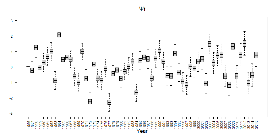
Figure 4: Boxplots of the posterior distributions of the annual random effects $\psi_{t}$ in $M_{4}$.

The posterior distributions at the observed locations of the four spatial processes in $M_{4}$, $\tilde{\beta}_{0}(\textbf{s}),\tilde{\alpha}(\textbf{s}),\rho_{Y}(\textbf{s})$, and $\sigma_{\epsilon}(\textbf{s})$, are summarized in Figure 5 using boxplots. The boxplots of the locations are sorted from the lowest to the highest elevation in the horizontal axis. They confirm the need to consider the four GPs to represent the great climatic variability of the region under study. To show the spatial behavior of the spatial processes over the entire region, maps of their posterior means, obtained by a model-based Bayesian kriging, are presented in Figure 6. In Section S3.2 of the Supplementary Materials, the parameters of $M_{4}$ are compared with the parameters of the local models described in Section S1.1, and both show good agreement.

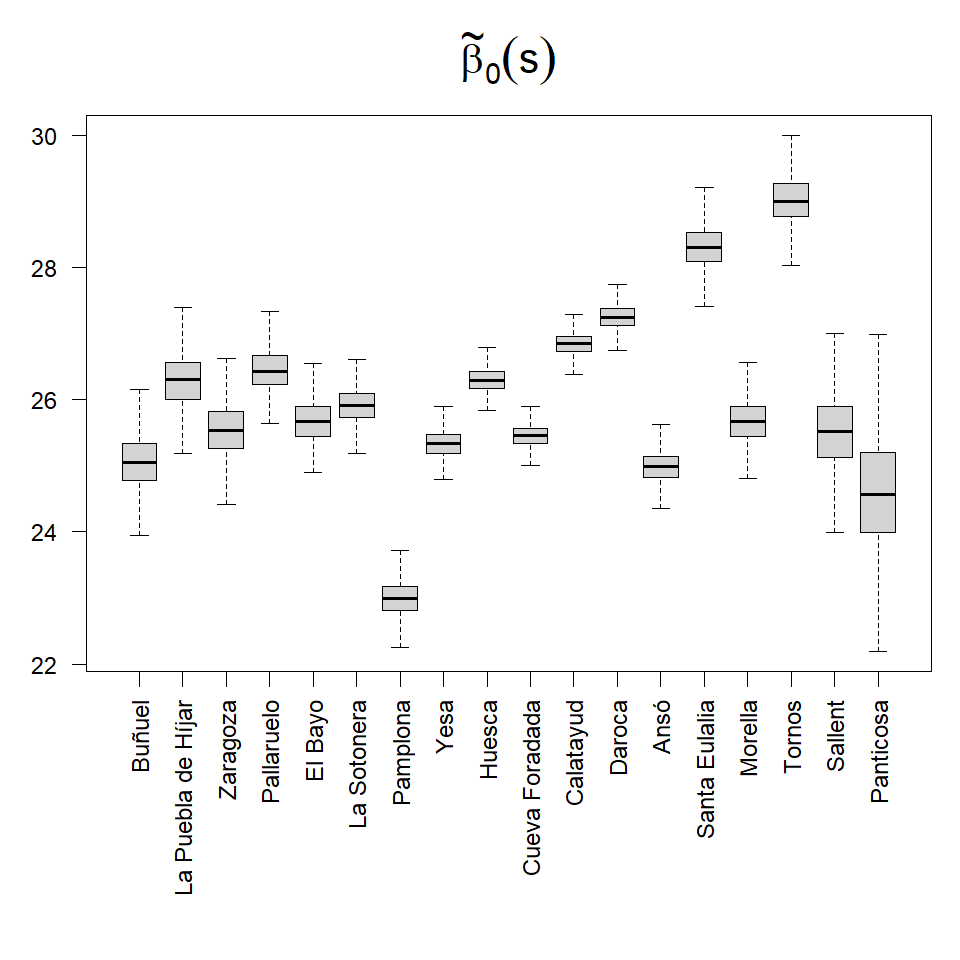
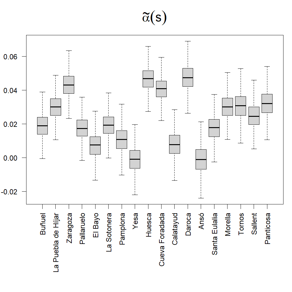
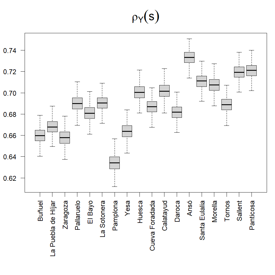
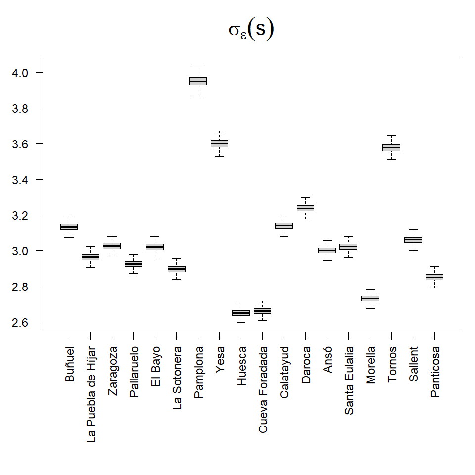
Figure 5: Boxplots of the posterior distributions of the spatial random effects, $\tilde{\beta}_{0}(\textbf{s}),\tilde{\alpha}(\textbf{s}),\rho_{Y}(\textbf{s}),\sigma_{\epsilon}(\textbf{s})$, in $M_{4}$. Locations are sorted by elevation, from lowest to highest.

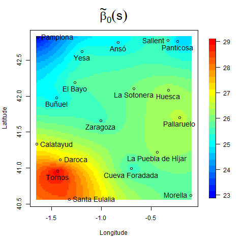
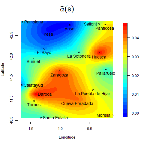
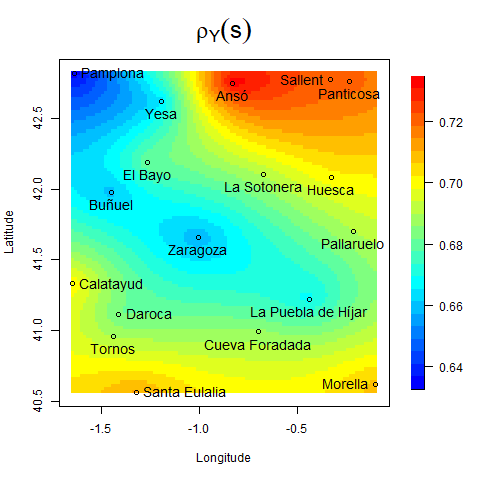
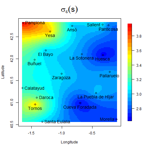
Figure 6: Maps of the posterior means of the four spatial processes included in $M_{4}$, obtained by a model-based Bayesian kriging, with resolution $100\times 100$.

The top-left plots in Figures 5 and 6 correspond to $\tilde{\beta}_{0}(\textbf{s})$. The posterior distributions for most of the locations show remarkable differences. In particular, $\tilde{\beta}_{0}(\textbf{s})$ has a clear climatic interpretation. The spatial adjustments provided by this GP help to improve the fit for the two areas with a similar elevation around 1,000 m but different climates. These areas are the southwest and the north of the region. The former has a warmer climate than the latter, whose climate is influenced by the proximity of the Atlantic Ocean.

With regard to the spatially varying yearly linear trend, $\tilde{\alpha}(\textbf{s})$, the top-right plots in Figures 5 and 6 reveal clear spatial differences in the warming trend. The posterior distributions for higher locations and for the Central Valley are shifted with respect to others. Most of the area shows warming trends, except some areas in the northwest, e.g., Yesa or Ansó, whose posterior distributions are centered at zero.

The spatial process for the autoregressive term, $\rho_{Y}(\textbf{s})$, is clearly necessary in the model. The bottom-left plot in Figure 5 shows that the posterior distributions for the 18 locations differ substantially. The posterior means of the $\rho_{Y}(\textbf{s})$ are positive in all locations and their values seem to have an increasing relation with the elevation. According to the bottom-left plot in Figure 6, the posterior mean is also related to cierzo, a severe northwesterly cold wind that gives rise to a renewal of the atmospheric condition with less warm air masses. This wind reduces the persistence of the temperature and therefore the dependence with respect to the previous day. In the areas affected by cierzo, the mean is around $0.65$, lower than the posterior mean of the mean of $\rho_{Y}(\textbf{s})$, close to $0.7$.

The need for the $\sigma_{\epsilon}(\textbf{s})$ process is also clear. The bottom-right plot in Figure 5 reveals strong differences among the posterior distributions of the standard deviations across locations. The high variability of Pamplona, Yesa and Tornos stands out. The bottom-right plot in Figure 6 confirms the spatial variability of the standard deviation and shows that higher standard deviations are observed in the western part of the region.

4.2.1 Prediction at unobserved locations

Now, we illustrate the use of the full model for prediction at three unobserved sites in the region: Longares (530 m), Olite (390 m), and Guara (800 m). The new sites are marked in red in Figure 1 and represent areas with different environmental and climatic characteristics. Longares is located in the southern half of the region in a rainfed agricultural area dedicated to the production of wine. Vines are seriously affected by global warming since high temperatures lead to both a decrease in production and a premature ripening of the grapes. Olite is located in a rural area in the northwest where smaller increases in the temperature have been observed; an incomplete series of observed values is available at this site. Guara is an uninhabited area in the Natural Park Sierra and Cañones de Guara. The prediction of the temperature evolution in this area is essential to better understand the changes that have been observed in the ecosystem of the Natural Park.

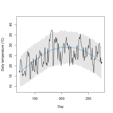
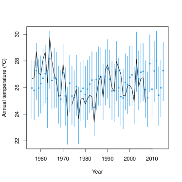
Figure 7: Left: Observed (black rough curve) and posterior predictive means (blue smooth curve) with associated $90\%$ credible intervals of daily maximum temperatures in Olite (1968). Right: Observed yearly averages (black curve) and associated posterior mean and $90\%$ credible intervals.

We use the model to impute missing values in an observed series using the posterior predictive distribution. Daily temperatures in Olite are available in the AEMET database from 1968 to 2007, although with many missing observations. As an example, Figure 7 shows the plot of the observed series and the posterior predictive means with $90\%$ credible intervals for MJJAS days in 1968 and, as a summary, the plot of the observed and the posterior yearly averages with $90\%$ credible intervals. The $90\%$ CVG in the observed data is $92.0\%$. The agreement between the observed and the predicted data confirms that $M_{4}$ can be used effectively to impute missing values in Olite.

The posterior distribution of the four spatial processes $\tilde{\beta_{0}}(\textbf{s})$, $\tilde{\alpha}(\textbf{s})$, $\rho_{Y}(\textbf{s})$, and $\sigma_{\epsilon}(\textbf{s})$ for the three predicted locations are shown in Figure S5 of the Supplementary Materials. The posterior distributions for $\tilde{\beta_{0}}(\textbf{s})$ in Longares and Guara are similar despite having different elevations. The posterior distributions of $\tilde{\alpha}(\textbf{s})$ in Longares and Guara are very similar while the distribution of Olite is shifted with a posterior mean almost $0.3^{\circ}$C per decade lower. The fitted $\rho_{Y}(\textbf{s})$’s show the differences in the autocorrelation of temperature in the three locations with posterior means varying from 0.65 to 0.72. The largest differences in the posterior distributions appear in the $\sigma_{\epsilon}(\textbf{s})$.

$M_{4}$ is also used to evaluate the change over time of the temperature in the three predicted sites, using the posterior predictive distribution of the difference between the average in the 30-year periods 1956–1985 and 1986–2015 (see Figure S6 in Supplementary Materials). Despite the difference in elevation, the posterior mean of the increment is similar in Longares and Guara, around $1.4^{\circ}$C, while in Olite it is smaller, $0.5^{\circ}$C and its $90\%$ credible interval $(-0.010,1.028)$ contains zero. The posterior probability that the mean in 1986–2015 is higher than in 1956–1985 is 0.94 in Olite and essentially 1 in Longares and Guara.

5 Summary and future work

We have proposed a very rich space-time mean model for daily maximum temperatures, fitted over a sixty year period for a region in Spain. Our specification is continuous in space and autoregressive in time. In time, autoregression was examined annually and also daily for the summer season within each year. We find novel spatial structure including spatially varying intercepts and trend coefficients as well as spatially varying autoregression coefficients and variances.

The proposed modeling can be adapted to other regions, perhaps considering other geographical covariates such as latitude, longitude or distance to the sea. Also, the modeling can omit spatial processes that are not necessary, e.g., avoiding $\rho_{Y}(\textbf{s})$ in a more homogeneous region with a lower variation in elevation. The modeling might also be adapted to other response variables in spatio-temporal problems, such as daily minimum temperature and other environmental variables including daily evapotranspiration or hourly temperature in the sea. The flexible autoregression terms can express behavior in series where serial correlation is an important source of variation.

A limitation of the present analysis is that we have only $18$ monitoring stations so that learning about the spatial surfaces in our modeling is less than we would want. Despite this small number of sites, the model has been able to capture the climate variability of the region under study. The spatial random effects identify areas with a different mean temperature level, but also areas where the observed warming over time shows a different trend, areas where temperature is more persistent (i.e., with a stronger daily serial correlation) or with different variability. The capacity of the fitted model to impute temperature over the entire region allows us to obtain reliable predictions and credible intervals for daily temperature series at unobserved sites. This can be valuable for economical, agricultural or environmental reasons.

Future work will consider different regions providing more available spatial locations $n$. However, the $\mathcal{O}(n^{3})$ computational complexity of inverting a $n\times n$ covariance matrix can be prohibitive for implementing the above model for data with large $n$. Reduced rank approximations to GPs may be used to address this computation bottleneck, e.g., Gaussian predictive process (Banerjee et al., 2008) or nearest-neighbour GP (Datta et al., 2016). As a different challenge, one may wonder whether the low trend values (blue region) in the top-right plot in Figure 6 are actually meaningful. Future work could implement a version of a spatially dependent multiple testing analysis (Risser et al., 2019) given the posterior draws of $\tilde{\alpha}(\textbf{s})$. A different future direction will move away from mean modeling to quantile modeling in order to investigate extremes of temperature, both hot and cold. This will lead to novel development for spatio-temporal quantile regression.

References

- AEMET (2011) AEMET (2011) Atlas climático ibérico – Iberian climate atlas. Ministerio de Medio Ambiente, y Medio Rural y Marino; Agencia Estatal de Meteorología; and Instituto de Meteorologia de Portugal, URL https://doi.org/10.31978/784-11-002-5
- Banerjee et al. (2008) Banerjee S, Gelfand AE, Finley AO, Sang H (2008) Gaussian predictive process models for large spatial data sets. Journal of the Royal Statistical Society: Series B (Statistical Methodology) 70(4):825–848, URL https://doi.org/10.1111/j.1467-9868.2008.00663.x
- Banerjee et al. (2014) Banerjee S, Carlin BP, Gelfand AE (2014) Hierarchical Modeling and Analysis for Spatial Data, 2nd edn. Chapman and Hall/CRC, New York, NY, USA, URL https://doi.org/10.1201/b17115
- Bopp and Shaby (2017) Bopp GP, Shaby BA (2017) An exponential-gamma mixture model for extreme Santa Ana winds. Environmetrics 28(8):e2476, URL https://doi.org/10.1002/env.2476
- Craigmile and Guttorp (2011) Craigmile PF, Guttorp P (2011) Space-time modelling of trends in temperature series. Journal of Time Series Analysis 32(4):378–395, URL https://doi.org/10.1111/j.1467-9892.2011.00733.x
- Datta et al. (2016) Datta A, Banerjee S, Finley AO, Gelfand AE (2016) Hierarchical nearest-neighbor Gaussian process models for large geostatistical datasets. Journal of the American Statistical Association 111(514):800–812, URL https://doi.org/10.1080/01621459.2015.1044091
- Diffenbaugh and Burke (2019) Diffenbaugh NS, Burke M (2019) Global warming has increased global economic inequality. Proceedings of the National Academy of Sciences 116(20):9808–9813, URL https://doi.org/10.1073/pnas.1816020116
- Gelfand et al. (1995) Gelfand AE, Sahu SK, Carlin BP (1995) Efficient parametrisations for normal linear mixed models. Biometrika 82(3):479–488, URL https://doi.org/10.1093/biomet/82.3.479
- Gneiting and Raftery (2007) Gneiting T, Raftery AE (2007) Strictly proper scoring rules, prediction, and estimation. Journal of the American Statistical Association 102(477):359–378, URL https://doi.org/10.1198/016214506000001437
- Hatfield et al. (2011) Hatfield JL, Boote KJ, Kimball BA, Ziska LH, Izaurralde RC, Ort D, Thomson AM, Wolfe D (2011) Climate impacts on agriculture: Implications for crop production. Agronomy Journal 103(2):351–370, URL https://doi.org/10.2134/agronj2010.0303
- IPCC (2013) IPCC (2013) Summary for policymakers. In: Stocker TF, Qin D, Plattner GK, Tignor M, Allen SK, Boschung J, Nauels A, Xia Y, Bex V, Midgley PM (eds) Climate Change 2013: The Physical Science Basis. Contribution of Working Group I to the Fifth Assessment Report of the Intergovernmental Panel on Climate Change, Cambridge University Press, Cambridge, United Kingdom and New York, NY, USA
- IPCC (2018) IPCC (2018) Summary for policymakers. In: Masson-Delmotte V, Zhai P, Pörtner HO, Roberts D, Skea J, Shukla PR, Pirani A, Moufouma-Okia W, Péan C, Pidcock R, Connors S, Matthews JBR, Chen Y, Zhou X, Gomis MI, Lonnoy E, Maycock T, Tignor M, Waterfield T (eds) Global warming of 1.5∘C. An IPCC Special Report on the impacts of global warming of 1.5∘C above pre-industrial levels and related global greenhouse gas emission pathways, in the context of strengthening the global response to the threat of climate change, sustainable development, and efforts to eradicate poverty, World Meteorological Organization, Geneva, Switzerland
- Lemos et al. (2007) Lemos RT, Sansó B, Los Huertos M (2007) Spatially varying temperature trends in a Central California Estuary. Journal of Agricultural, Biological, and Environmental Statistics 12(3):379, URL https://doi.org/10.1198/108571107X227603
- Li et al. (2020) Li S, Griffith DA, Shu H (2020) Temperature prediction based on a space-time regression-kriging model. Journal of Applied Statistics 47(7):1168–1190, URL https://doi.org/10.1080/02664763.2019.1671962
- Mohammadi et al. (2021) Mohammadi B, Mehdizadeh S, Ahmadi F, Lien NTT, Linh NTT, Pham QB (2021) Developing hybrid time series and artificial intelligence models for estimating air temperatures. Stochastic Environmental Research and Risk Assessment 35(6):1189–1204, URL https://doi.org/10.1007/s00477-020-01898-7
- Navarro-Serrano et al. (2018) Navarro-Serrano F, López-Moreno JI, Azorin-Molina C, Alonso-González E, Tomás-Burguera M, Sanmiguel-Vallelado A, Revuelto J, Vicente-Serrano SM (2018) Estimation of near-surface air temperature lapse rates over continental Spain and its mountain areas. International Journal of Climatology 38(8):3233–3249, URL https://doi.org/10.1002/joc.5497
- Peña-Angulo et al. (2021) Peña-Angulo D, Gonzalez-Hidalgo JC, Sandonís L, Beguería S, Tomas-Burguera M, López-Bustins JA, Lemus-Canovas M, Martin-Vide J (2021) Seasonal temperature trends on the Spanish mainland: A secular study (1916–2015). International Journal of Climatology 41(5):3071–3084, URL https://doi.org/10.1002/joc.7006
- Reich et al. (2014) Reich BJ, Shaby BA, Cooley D (2014) A hierarchical model for serially-dependent extremes: A study of heat waves in the western US. Journal of Agricultural, Biological and Environmental Statistics 19(1):119–135, URL https://doi.org/10.1007/s13253-013-0161-y
- Risser et al. (2019) Risser MD, Paciorek CJ, Stone DA (2019) Spatially dependent multiple testing under model misspecification, with application to detection of anthropogenic influence on extreme climate events. Journal of the American Statistical Association 114(525):61–78, URL https://doi.org/10.1080/01621459.2018.1451335
- Roldán et al. (2016) Roldán E, Gómez M, Pino MR, Pórtoles J, Linares C, Díaz J (2016) The effect of climate-change-related heat waves on mortality in Spain: uncertainties in health on a local scale. Stochastic Environmental Research and Risk Assessment 30(3):831–839, URL https://doi.org/10.1007/s00477-015-1068-7
- Rossati (2017) Rossati A (2017) Global warming and its health impact. The International Journal of Occupational and Environmental Medicine 8(1):7–20, URL https://doi.org/10.15171/ijoem.2017.963
- Sahu et al. (2006) Sahu SK, Gelfand AE, Holland DM (2006) Spatio-temporal modeling of fine particulate matter. Journal of Agricultural, Biological, and Environmental Statistics 11(1):61–86, URL https://doi.org/10.1198/108571106X95746
- Sahu et al. (2007) Sahu SK, Gelfand AE, Holland DM (2007) High-resolution space-time ozone modeling for assessing trends. Journal of the American Statistical Association 102(480):1221–1234, URL https://doi.org/10.1198/016214507000000031
- Schlenker and Roberts (2009) Schlenker W, Roberts MJ (2009) Nonlinear temperature effects indicate severe damages to U.S. crop yields under climate change. Proceedings of the National Academy of Sciences 106(37):15594–15598, URL https://doi.org/10.1073/pnas.0906865106
- Verdin et al. (2015) Verdin A, Rajagopalan B, Kleiber W, Katz RW (2015) Coupled stochastic weather generation using spatial and generalized linear models. Stochastic Environmental Research and Risk Assessment 29(2):347–356, URL https://doi.org/10.1007/s00477-014-0911-6
- Watts et al. (2015) Watts N, Adger WN, Agnolucci P, Blackstock J, Byass P, Cai W, Chaytor S, Colbourn T, Collins M, Cooper A, Cox PM, Depledge J, Drummond P, Ekins P, Galaz V, Grace D, Graham H, Grubb M, Haines A, Hamilton I, Hunter A, Jiang X, Li M, Kelman I, Liang L, Lott M, Lowe R, Luo Y, Mace G, Maslin M, Nilsson M, Oreszczyn T, Pye S, Quinn T, Svensdotter M, Venevsky S, Warner K, Xu B, Yang J, Yin Y, Yu C, Zhang Q, Gong P, Montgomery H, Costello A (2015) Health and climate change: policy responses to protect public health. The Lancet 386(10006):1861–1914, URL https://doi.org/10.1016/S0140-6736(15)60854-6
- WMO (2017) WMO (2017) WMO Guidelines on the Calculation of Climate Normals (WMO-No. 1203). Geneva, Switzerland, URL https://library.wmo.int/doc_num.php?explnum_id=4166
- Zhang (2004) Zhang H (2004) Inconsistent estimation and asymptotically equal interpolations in model-based geostatistics. Journal of the American Statistical Association 99(465):250–261, URL https://doi.org/10.1198/016214504000000241