Iterated integrals and multiple polylogarithm at algebraic arguments

Abstract.

We give systematic method that can convert many values of multiple polylogarithm at algebraic arguments into colored multiple zeta values (CMZV). Moreover, a new method to generate nonstandard relations of CMZVs is discovered. Some applications to polylogarithm identities and infinite series are also mentioned.

1. Introduction

In this paper, we will denote

$$\operatorname{Li}_{s_{1},\cdots,s_{k}}(a_{1},\cdots,a_{k})=\sum_{n_{1}>\cdots>n_{k}\geq 1}\frac{a_{1}^{n_{1}}\cdots a_{k}^{n_{k}}}{n_{1}^{s_{1}}\cdots n_{k}^{s_{k}}}$$

to be the multiple polylogarithm. Here $k$ is called the depth and $s_{1}+\cdots+s_{k}$ is called the weight.

When $a_{i}$ are $N$-th roots of unity, $s_{i}$ are positive integers and $(a_{i},s_{i})\neq(1,1)$, $\operatorname{Li}_{s_{1},\cdots,s_{k}}(a_{1},\cdots,a_{k})$ is called a colored multiple zeta values (CMZV) of weight $s_{1}+\cdots+s_{k}$ and level $N$. Denote the $\mathbb{Q}$-span of weight $w$ and level $N$ CMZVs by $\textsf{CMZV}^{N}_{w}$. The special case when all $a_{i}=1$ is the well-known multiple zeta function. The special case when $a_{2}=\cdots=a_{k}=1$ is generalized polylogarithm, and denoted by $\operatorname{Li}_{s_{1},\cdots,s_{k}}(a_{1})$.

There have been a lot of researches on $\textsf{CMZV}^{N}_{w}$, including its algebraic properties ([3], [17]), relations satisfied by them ([28], [20], [29]) , and its motivic $\mathbb{Q}$-dimension. ([15], [14]).

On the other hand, researches on multiple polylogarithm in general is more scarce. Most of them concentrate on analytic aspects such as monodromy. For their special values, most of them concentrate on the case when $a_{i}$ are roots of unity (e.g. [5], [7]), as those for general $a_{i}$’s are deemed too board. In the paper, we take on this endeavor, as an application to the theory developed in Section 3, we will prove that, among many others, that ($s_{1}+\cdots+s_{n}=w$),

• The multiple polylogarithm $\operatorname{Li}_{s_{1},\cdots,s_{n}}(x_{1},\cdots,x_{n})\in\textsf{CMZV}^{5}_{w}$ if at most two of $x_{i}=(\sqrt{5}-1)/2$ and remaining $x_{i}=1$.

• The generalized polylogarithm $\operatorname{Li}_{s_{1},\cdots,s_{n}}(z)\in\textsf{CMZV}^{6}_{w}$ if $z=\frac{-1}{2},\frac{1}{3},\frac{1}{4},\frac{1}{9}$

• The multiple polylogarithm $\operatorname{Li}_{s_{1},\cdots,s_{n}}(x_{1},\cdots,x_{n})\in\textsf{CMZV}^{6}_{w}$ if at most two of $x_{i}=-1/2$ and remaining $x_{i}=1$; if "at most two" is changed into "at most three", then it is in $\textsf{CMZV}^{12}_{w}$.

• The generalized polylogarithm $\operatorname{Li}_{s_{1},\cdots,s_{n}}(z)\in\textsf{CMZV}^{8}_{w}$ if $z=1-\sqrt{2},\frac{4-3\sqrt{2}}{8}$

which are not obvious from the very definition of $\textsf{CMZV}^{N}_{w}$.

We give three main applications of our theory and techniques:

1. Non-standard relations of CMZVs There exists so-called nonstandard relations of CMZVs [28], which are missing relations after all known ones had been adjoined. Generally intractable, their nature remains elusive, we unveil a portion of them in Section 5. We succeed in finding all $\mathbb{Q}$-between CMZVs for levels and weights mentioned in 5.2.

2. Polylogarithm identities We apply the theory developed in Section 3, and our ability to find all putative $\mathbb{Q}$-relations between CMZVs, to classical polylogarithm identities. In particular, we will give a conceptual and effective computable proof of Coxeter’s famous ladder

   $$\text{Li}_{2}\left(\rho^{20}\right)=2\text{Li}_{2}\left(\rho^{10}\right)+15\text{Li}_{2}\left(\rho^{4}\right)-10\text{Li}_{2}\left(\rho^{2}\right)+\frac{\pi^{2}}{5}\qquad\rho=(\sqrt{5}-1)/2$$

3. Apéry-like series We will give alternative proofs to an abundance of such series in last section, using a uniform method, series that succumb under our attacks include

   $$\sum_{n=1}^{\infty}\frac{(-1)^{n-1}\left(10H_{n}-\frac{3}{n}\right)}{n^{3}\binom{2n}{n}}=\frac{\pi^{4}}{30}$$

   $$\sum_{n=1}^{\infty}\frac{-102H_{n}+3H_{2n}+\frac{28}{n}}{n^{4}\binom{2n}{n}}=-\frac{55}{18}\pi^{2}\zeta(3)$$

   $$\sum_{n=1}^{\infty}\frac{H_{2n}-H_{n}}{\binom{3n}{n}\left(2^{n}n^{2}\right)}=-\frac{\pi C}{2}+\frac{33\zeta(3)}{32}+\frac{1}{24}\pi^{2}\log(2)$$

2. Preliminaries

2.1. Iterated integral

We quickly assemble required facts of iterated integral ([11], [16]). Let functions $f_{i}(t)$ defined on $[a,b]$, define inductively

$$\int_{a}^{b}f_{1}(t)dt\cdots f_{n}(t)dt=\int_{a}^{b}f_{1}(u)du\cdots f_{n-1}(u)\int_{a}^{u}f_{n}(t)dt$$

When $n=1$, this is the usual definite integral of $\int_{a}^{b}f_{1}(t)dt$. When $r=0$, define its value to be $1$.

The definition can be extended to manifold. Let $\gamma:[0,1]\to M$ a path on a manifold $M$, $\omega_{1},\cdots,\omega_{n}$ be differential $1$-forms on $M$. Then

$$\int_{\gamma}\omega_{1}\cdots\omega_{n}:=\int_{0}^{1}f_{1}(t)dt\cdots f_{r}(t)dt$$

with $\gamma^{\ast}\omega_{i}=f_{i}(t)dt$ being the pullback of $\omega$. Then if $f:N\to M$ is a differentible map between two manifolds $N$ and $M$,

(2.1) $$\int_{f\circ\gamma}\omega_{1}\cdots\omega_{n}=\int_{\gamma}f^{\ast}\omega_{1}\cdots f^{\ast}\omega_{n}$$

Proposition 2.1.

Iterated integral enjoys the following properties:

$$\int_{\gamma}\omega_{1}\cdots\omega_{n}=(-1)^{n}\int_{\gamma^{-1}}\omega_{n}\cdots\omega_{1}$$

where $\gamma^{-1}$ is the reverse path of $\gamma$.

$$\int_{\gamma_{1}\gamma_{2}}\omega_{1}\cdots\omega_{n}=\sum_{r=0}^{n}\int_{\gamma_{1}}\omega_{1}\cdots\omega_{r}\int_{\gamma_{2}}\omega_{r+1}\cdots\omega_{n}$$

where $\gamma_{2}(1)=\gamma_{1}(0)$, here $\gamma_{1}\gamma_{2}$ means composition of two paths, first $\gamma_{2}$, then $\gamma_{1}$.

(2.2) $$\int_{\gamma}\omega_{1}\cdots\omega_{n}\int_{\gamma}\omega_{n+1}\cdots\omega_{n+m}=\sum_{\begin{subarray}{c}\sigma\in S_{n+m}\\ \sigma(1)<\cdots<\sigma(n)\\ \sigma(n+1)<\cdots<\sigma(n+m)\end{subarray}}\int_{\gamma}\omega_{\sigma^{-1}(1)}\cdots\omega_{\sigma^{-1}(n+m)}$$

the last sum is over certain elements of symmetric group $S_{n+m}$, it can also be viewed as shuffle product between $\omega_{1}\cdots\omega_{n}$ and $\omega_{n+1}\cdots\omega_{n+m}$, as defined in next subsection.

Let $X$ be a set, $\mathbb{Q}\langle X\rangle$ be the free non-commutative polynomial algebra over $\mathbb{Q}$ generated by $X$, let $\mathbb{Q}\llangle X\rrangle$ be the completion of $\mathbb{Q}\langle X\rangle$. Treating $X$ as set of alphabets, let $X^{*}$ be the set of words (including the empty word) over $X$.

Define a binary operation $\shuffle$ on $\mathbb{Q}\langle X\rangle$ via:

$$w\shuffle 1=1\shuffle w=w\qquad xw\shuffle yv=x(w\shuffle yv)+y(xu\shuffle v)$$

for $w,v\in X^{\ast},x,y\in X$. Then distribute $\shuffle$ over addition and scalar multiplication. The shuffle product is commutative and associative.

Using shuffle product, the last property 2.2 of iterated integral can be written as

$$\int_{\gamma}\omega_{1}\cdots\omega_{n}\int_{\gamma}\omega_{n+1}\cdots\omega_{n+m}=\int_{\gamma}\omega_{1}\cdots\omega_{n}\shuffle\omega_{n+1}\cdots\omega_{n+m}$$

If each element of $X$ is a differential 1-form on a manifold $M$, let

$$\textbf{I}_{\gamma}(X)=\sum_{w\in X^{\ast}}\int_{\gamma}w\in\mathbb{C}\llangle X\rrangle$$

If $\gamma_{1},\gamma_{2}$ be two paths on $M$ with $\gamma_{1}(1)=\gamma_{2}(0)$, then $\textbf{I}_{\gamma_{2}\gamma_{1}}(X)=\textbf{I}_{\gamma_{2}}(X)\textbf{I}_{\gamma_{1}}(X)$, here RHS is the (concatenation) multiplication on $\mathbb{C}\llangle X\rrangle$. For constant path $\gamma$, $\textbf{I}_{\gamma}(X)=1$. When the set of differential form $X$ is clear from context, we will simply write $\textbf{I}_{\gamma}$.

If each of the differential 1-form in $X$ is closed, then the iterated integral is a homotopy (with endpoints fixed) invariant. For $x_{0}\in X$, we therefore obtain a homomorphism $\pi_{1}(M,x_{0})\to\mathbb{C}\llangle X\rrangle$, defined via $[\gamma]\to\textbf{I}_{\gamma}$.

2.2. Multiple polylogarithm

Denote the multiple polylogarithm as

$$\operatorname{Li}_{s_{1},\cdots,s_{k}}(x_{1},\cdots,x_{k})=\sum_{s_{1}>\cdots>s_{k}\geq 1}\frac{x_{1}^{n_{1}}\cdots x_{k}^{n_{k}}}{n_{1}^{s_{1}}\cdots n_{k}^{s_{k}}}$$

the series converges if $|x_{1}\cdots x_{i}|<1$ for $i\leq k$. Also denote $\omega(a)$ to be the differential form $dx/(x-a)$. Then it’s easy to see that

(2.3) $$\operatorname{Li}_{s_{1},\cdots,s_{k}}(x_{1},\cdots,x_{k})=(-1)^{k}\int_{0}^{1}\omega(0)^{s_{1}-1}\omega(a_{1})\cdots\omega(0)^{s_{d}-1}\omega(a_{d})\qquad a_{i}=x_{1}^{-1}\cdots x_{i}^{-1}$$

We will have the occasion to use the generalized polylogarithm,

$$\operatorname{Li}_{s_{1},\cdots,s_{k}}(x):=\operatorname{Li}_{s_{1},\cdots,s_{k}}(x_{1},1,\cdots,1)=\sum_{n=1}^{\infty}\frac{x^{n}}{n^{s_{1}}}H_{s_{2},\cdots,s_{k}}(n)$$

In particular, the ordinary polylogarithm $\operatorname{Li}_{s}(x)=\sum_{n=1}^{\infty}x^{n}/n^{s}$ is a special case of this.

A central question of the following section is to study for which $\{a_{1},\cdots,a_{n}\}$, the iterated integral

$$\int_{0}^{1}\omega(a_{1})\cdots\omega(a_{n})$$

(when convergent, i.e. $a_{1}\neq 1,a_{n}\neq 0$ and none of $0<a_{i}<1$) lies in $\textsf{CMZV}^{N}_{n}$ for some level $N$. It is evident that, from (2.3), this is true when each $a_{i}$ is an $N$-th root of unity. On the other hand, there is not obvious there is any other such values $\{a_{1},\cdots,a_{n}\}$. We will see in the next section that there is in fact a lot of them, for example, when $\{a_{1},\cdots,a_{n}\}\subset\{0,1,2,3\}$, it is in $\textsf{CMZV}^{6}_{n}$; when $\{a_{1},\cdots,a_{n}\}\subset\{0,1,(\sqrt{5}+1)/2\}$, it is in $\textsf{CMZV}^{5}_{n}$.

2.3. Graded algebra

Let $R=\oplus_{m\geq 0}R_{m}$ be a commutative graded algebra over a field $k=R_{0}$, with $h_{k}=\dim_{k}R_{k}<\infty$. Let

$$\overline{R}_{m}=\sum_{n<m}R_{n}R_{m-n}$$

Let $\sum_{m=0}^{\infty}c_{m}t^{m}=\log\left(1+\sum_{m=1}^{\infty}h_{m}t^{m}\right)$, then

(2.4) $$\dim_{k}R_{m}/\overline{R}_{m}=\sum_{k\mid m}\frac{\mu(k)}{k}c_{m/k}$$

Moreover, for a set of letters $X$, $\textbf{I}\in R\llangle X\rrangle$, with coefficient of degree $d$ word being in $R_{d}$, we define a $k$-linear function $R\llangle X\rrangle\to R,\omega\mapsto\textbf{I}[\omega]$ which maps a homogeneous word to its coefficient in I. It is easy to check that

$$(\textbf{I}_{1}\cdots\textbf{I}_{n})[\omega]\equiv\textbf{I}_{1}[\omega]+\cdots+\textbf{I}_{n}[\omega]\pmod{\overline{R}_{m}}$$

if $\omega$ is degree $m$ homogeneous.

2.4. Regularization

Denote $R:=\mathbb{C}\llangle X\rrangle$ in this subsection. $\mathbb{C}\langle X\rangle$ and its completion $R$ has a Hopf algebra structure, comultiplication is defined by $\Delta(x_{i})=x_{i}\otimes 1+1\otimes x_{i}$ and antipole $S$ is $S(x_{1}\cdots x_{n})=(-1)^{n}x_{n}\cdots x_{1}$ for $x_{i}\in X$.

Let $x_{1},x_{2}$ be two elements of $X$, we have quotient maps: $\pi_{1}:R\to R/(x_{1}R),\pi_{1,2}:R\to R/(x_{1}R+Rx_{2})$. The Hopf algebra structure of $R$ descends into the quotient.

Proposition 2.2.

(a) Every group-like element in $\pi_{1}(R)$ is the image of some group-like elements in $R$ under $\pi_{1}$. Moreover, any two such elements $\Phi_{1},\Phi_{2}$ are related by

$$\Phi_{2}=\exp(Ax_{1})\Phi_{1}$$

for some $A\in\mathbb{C}$.

(b) Every group-like element in $\pi_{1,2}(R)$ is the image of some group-like elements in $R$ under $\pi_{1,2}$. Moreover, any two such elements $\Phi_{1},\Phi_{2}$ are related by

$$\Phi_{2}=\exp(Ax_{1})\Phi_{1}\exp(Bx_{2})$$

for some $A,B\in\mathbb{C}$.

Proof.

See [30] and [21]. ∎

Let $\mathbf{J}\in R/(x_{1}R+Rx_{2})$ be group-like, $\mathbf{I}$ be its unique group-like lift to $R$ with coefficient of $x_{1},x_{2}$ being zero, then coefficient of $\mathbf{I}$ can be calculated recursively as follows:

let $k,m,n\geq 0$ be integers, $\xi_{i}\in X,\xi_{1}\neq x_{1},\xi_{k}\neq x_{2}$, set $\xi_{1}\cdots\xi_{k}x_{2}^{n}=\xi_{1}\cdots\xi_{q}$,

(2.5) $$\textbf{I}[x_{1}^{m}\xi_{1}\cdots\xi_{k}x_{2}^{n}]=\begin{cases}0\qquad&\text{ if }mn=k=0\\ \textbf{I}[\xi_{1}\cdots\xi_{k}]\qquad&\text{ if }m=n=0\\ -\frac{1}{m}\sum_{i=1}^{q}\textbf{I}[x_{1}^{m-1}\xi_{1}\cdots\xi_{i}x_{1}\xi_{i+1}\cdots\xi_{q}]\qquad&\text{ if }m>0\\ -\frac{1}{n}\sum_{i=1}^{k}\textbf{I}[\xi_{1}\cdots\xi_{i-1}x_{2}\xi_{i+1}\cdots\xi_{k}x_{2}^{n-1}]\qquad&\text{ if }m=0,n>0\end{cases}$$

here we write $\textbf{I}[\omega]$ to mean the coefficient of $\omega$ in I

When elements of $X$ are 1-forms on a manifold $M$, $\textbf{I}_{\gamma}(X)$ is a group-like element of $R$, i.e. $\Delta(\textbf{I}_{\gamma}(X))=\textbf{I}_{\gamma}(X)\otimes\textbf{I}_{\gamma}(X)$, this is actually equivalent to the definition of shuffle product.

We next record here some observations that will be used in next section. Denote

$$X=\{\omega(0),\omega(1),\omega(c_{1}),\cdots,\omega(c_{n})\}$$

be 1-forms on $\mathbb{C}$, let $\gamma:[0,1]\to\mathbb{C},x\mapsto x$ be a path that goes from $0$ to $1$ and $c_{i}$ does not lie between $0$ and $1$. For $\textbf{I}_{\varepsilon}\in R$, we write $\textbf{I}_{\varepsilon}=O(\varepsilon)$ if each coefficient is $O(\varepsilon)$ as $\varepsilon\to 0$, similarly, we write $\textbf{I}_{\varepsilon}=o(1)$ if each coefficient is $o(1)$.

For $\gamma$ as above, let $\gamma(\varepsilon)$ be the restriction of $\gamma$ on $(\varepsilon,1-\varepsilon)$. Let $\pi$ be the map $R/(\omega(1)R+R\omega(0))$, then $\textbf{J}=\lim_{\varepsilon\to 0}\pi(\textbf{I}_{\gamma(\varepsilon)}(X))$ exists, and is group-like in $\pi(R)$, let $\tilde{\textbf{I}}$ be the unique group-like element of $R$ that maps to J, with coefficient of $\omega(1),\omega(0)$ being $0$.

Lemma 2.3.

As $\varepsilon\to 0$,

$$\textbf{I}_{\gamma(\varepsilon)}=e^{(\log\varepsilon)\omega(1)}\tilde{\textbf{I}}e^{(-\log\varepsilon)\omega(0)}+O(\varepsilon^{1/2})$$

Proof.

We abberiviate $\textbf{I}_{\gamma(\varepsilon)}$ by $\textbf{I}_{\varepsilon}$. By definition of $\mathbf{J}$, we have $\pi(\textbf{I}_{\varepsilon})=\textbf{J}+o(1)$, however, all terms of $\pi(\textit{I}_{\varepsilon})$ are convergent iterated integral, therefore by (2.3), they are analytic at $\varepsilon=0$, so the $o(1)$ term is actually $O(\varepsilon)$. On other hand, so we have $\pi(\textbf{I}_{\varepsilon})=\pi(\tilde{\textbf{I}}+O(\varepsilon))=\textbf{J}+O(\varepsilon)$, so $\tilde{\textbf{I}}$ and $\mathbf{I}_{\varepsilon}$ map to same element under $\pi$, so by proposition above, there exists $A_{\varepsilon},B_{\varepsilon}$ such that

$$\textbf{I}_{\gamma(\varepsilon)}=e^{A_{\varepsilon}\omega(1)}(\tilde{\textbf{I}}+O(\varepsilon))e^{B_{\varepsilon}\omega(0)}$$

by choice of $\tilde{\textbf{I}}$, its coefficient of $\omega(0),\omega(1)$ are zero, so

$$A_{\varepsilon}=\int_{\varepsilon}^{1-\varepsilon}\omega(1)+O(\varepsilon)=\int_{\varepsilon}^{1-\varepsilon}\frac{dx}{x-1}+O(\varepsilon)=\log\varepsilon+O(\varepsilon)$$

similarly for $B_{\varepsilon}=-\log\varepsilon+O(\varepsilon)$. The term $e^{A_{\varepsilon}\omega(1)}O(\varepsilon)e^{B_{\varepsilon}\omega(0)}$ contributes $O(\varepsilon)^{1/2}$, completing the proof. ∎

Lemma 2.4.

Using notations above, let $\rho(\varepsilon)$ be a section of arc of the circle, centered at $c_{1}$ and of radius $\varepsilon$, then $\lim_{\varepsilon\to 0}\textbf{I}_{\rho(\varepsilon)}(X)=\exp(A\omega(c_{1}))$ for some $A\in\mathbb{C}$.

Proof.

Can assume WLOG $c_{1}=0$. Recall that $\textbf{I}_{\rho(\varepsilon)}(X)=\sum_{\omega\in X^{\ast}}(\int_{\rho(\varepsilon)}\omega)\omega$, when $\omega$ contain any letter other than $\omega(0)$, the integral as $\varepsilon$ converges to $0$, indeed, pullback by $f:\varepsilon e^{i\theta}$, $f^{\ast}\omega(0)=id\theta$ and $f^{\ast}\omega(a)=re^{i\theta}/(re^{i\theta}-a)d\theta$ which converges uniformly to $0$ if $a\neq 0$, so

$$\int_{\rho(\varepsilon)}\omega(0)\cdots\omega(a)\cdots\omega(0)=\int_{0}^{\theta}f^{\ast}\omega(0)\cdots f^{\ast}\omega(a)\cdots f^{\ast}\omega(0)\to 0$$

If $\omega=\omega(0)^{n}$ contains only $\omega(0)$, then above implies

$$\int_{\rho(\varepsilon)}\omega(0)^{n}=\int_{0}^{\theta}(id\theta)^{n}=\frac{i^{n}\theta^{n}}{n!}$$

∎

Lemma 2.5.

Let $\rho(R)$ be a section of arc of the circle, centered at $c_{1}$ and of radius $R\to\infty$, $X=\{\omega(a_{1}),\cdots,\omega(a_{k})\}$ then $\lim_{R\to\infty}\textbf{I}_{\rho(R)}(X)=\exp(A(\omega(a_{1})+\cdots+\omega(a_{k})))$ for some $A\in\mathbb{C}$.

Proof.

Pullback by $f:Re^{i\theta}$, $f^{\ast}\omega(a)=Re^{i\theta}/(Re^{i\theta}-a)d\theta$ which converges uniformly to $1$ if $R\to\infty$, so

$$\int_{\rho(R)}\omega(c_{1})\cdots\omega(c_{n})=\int_{0}^{\theta}f^{\ast}\omega(c_{1})\cdots f^{\ast}\omega(c_{n})\to\frac{\theta^{n}}{n!}$$

which matches the coefficients of $\exp(A(\omega(a_{1})+\cdots+\omega(a_{k})))$ with $A=\theta$. ∎

3. Iterated integral of general base

In this section, we let $\omega(a)$ to be the differential form $dx/(x-a)$. Also denote $\omega(\infty)=0$, with this definition, one checks that, for any mobius transformation $R:\hat{\mathbb{C}}\to\hat{\mathbb{C}}$ and any $a\in\hat{\mathbb{C}}$, one has

$$R^{\ast}\omega(a)=\frac{R^{\prime}}{R-a}dx=\omega(R^{-1}(a))-\omega(R^{-1}(\infty))$$

Now recall our notation of iterated integral $\int_{\gamma}\omega(a_{1})\cdots\omega(a_{n})$ for $a_{i}\in\mathbb{C}$ with $\gamma:[0,1]\to\mathbb{C}$. If the path $\gamma$ does not pass through any of $a_{i}$ and the start $\gamma(0)\neq a_{n}$ and end $\gamma(1)\neq a_{1}$, the iterated integral converges, so equals a complex number. Consider the following iterated integral, with $\gamma$ now a path in extended complex plane $\hat{\mathbb{C}}$, assume $\gamma(0,1)$ (image of $\gamma$ under the open interval) does not contain $c_{i}$ and $d_{i}$, consider

(3.1) $$\int_{\gamma}(\omega(c_{1})-\omega(d_{1}))(\omega(c_{2})-\omega(d_{2}))\cdots(\omega(c_{n})-\omega(d_{n}))\qquad c_{i},d_{i}\in\hat{\mathbb{C}}$$

here each differential is $(1/(x-c_{i})-1/(x-d_{i}))dx$. We note here that the above integral makes sense (i.e. equals a well-defined complex number) if

(3.2) $$\gamma(0)\neq c_{n},d_{n}\qquad\gamma(1)\neq c_{1},d_{1}$$

Indeed, if $\gamma$ completely lie in $\mathbb{C}$ and $c_{i},d_{i}\in\mathbb{C}$, this is already noted in previous paragraph, for the case involving $\infty$, the integral still converge since $1/(x-a)-1/(x-b)=O(1/x^{2})$.

Now we define the central object of our discussion:

Definition 3.1.

Let $S$ be a finite subset of $\hat{\mathbb{C}}$, for positive integer $n$, define the $\mathbb{Q}$-vector subspace $\textsf{MZV}^{S}_{n}$ of $\mathbb{C}$ as the $\mathbb{Q}$-span of all possible (*), with $c_{i},d_{i}$ ranges over all elements of $S$ and $\gamma$ ranges over all paths in $\hat{\mathbb{C}}$ with

$$\gamma(0),\gamma(1)\in S\qquad\gamma(0)\neq c_{n},d_{n}\qquad\gamma(1)\neq c_{1},d_{1}$$

We call $n$ the weight of $\textsf{MZV}^{S}_{n}$.

We will soon see $\textsf{MZV}^{S}_{n}$ is a very natural object of investigation. Note that trivially if $S$ has less than 3 elements, then the space $\textsf{MZV}^{S}_{n}$ is zero. So we always assume that $|S|\geq 3$. We first record some obvious consequences:

Proposition 3.2.

Assume $|S|\geq 3$, and let $R$ be a rational function

1. $2\pi i\in\textsf{MZV}^{S}_{1}$

2. $\textsf{MZV}^{S}_{n}\textsf{MZV}^{S}_{m}\subset\textsf{MZV}^{S}_{n+m}$

3. If $R^{-1}(R(S))\subset S$, then $\textsf{MZV}^{R(S)}_{n}\subset\textsf{MZV}^{S}_{n}$

4. If $R$ is invertible, then $\textsf{MZV}^{R(S)}_{n}=\textsf{MZV}^{S}_{n}$.

Proof.

(1) Let $a,b,c$ be three distinct points of $S$, consider the integral $\int_{\gamma}(\omega(b)-\omega(c))$ with $\gamma$ a circle starting and ending at $a$, enclosing only $b$ but not $c$, the value of the integral is then $\pm 2\pi i$, so this is in $\textsf{MZV}^{S}_{1}$.

(2) This is a direct consequence of shuffle product, by treating $\omega(c_{i})-\omega(d_{i})$ as alphabet.

(3) We note the following, if $R$ is any rational function (not necessarily of degree $1$) we still have

$$R^{\ast}\omega(a)=\frac{R^{\prime}}{R-a}dx=\omega(R^{-1}(a))-\omega(R^{-1}(\infty))\qquad a\in\hat{\mathbb{C}}$$

but now we interpret the term $\omega(R^{-1}(a)):=\sum_{R(a_{i})=a}\omega(a_{i})$ counted with multiplicity.

Therefore we have

$$R^{\ast}(\omega(a)-\omega(b))=\omega(R^{-1}(a))-\omega(R^{-1}(b))$$

by canceling $\omega(R^{-1}(\infty))$

Let $a,b\in S$, let $\gamma$ be any path from $R(a)$ to $R(b)$ for which

(3.3) $$R(a)\neq R(c_{n}),R(d_{n})\qquad R(b)\neq R(c_{1}),R(d_{1})$$

let the integral

$$I:=\int_{\gamma}(\omega(R(c_{1}))-\omega(R(d_{1})))(\omega(R(c_{2}))-\omega(R(d_{2})))\cdots(\omega(R(c_{n}))-\omega(R(d_{n})))$$

we need to show $I\in\textsf{MZV}^{S}_{n}$. Now $R$ can be treated as a covering map from $\hat{\mathbb{C}}$ minus preimage of ramified points, from which it is easy to see there exists a path (not necessarily unique) $\gamma_{0}$, starting at $a$ and ending at $b$, such that $R\circ\gamma_{0}=\gamma$. So we have, by the pullback property of iterated integral,

$$I =\int_{\gamma_{0}}(R^{\ast}\omega(R(c_{1}))-R^{\ast}\omega(R(d_{1})))\cdots(R^{\ast}\omega(R(c_{n}))-R^{\ast}\omega(R(d_{n})))$$

$$=\int_{\gamma_{0}}(\omega(R^{-1}(R(c_{1})))-\omega(R^{-1}(R(d_{1}))))\cdots(\omega(R^{-1}(R(c_{n})))-\omega(R^{-1}(R(d_{n}))))$$

if degree of $R$ is $l$, then each of term in integral above can be written as sum of $l$ terms of form $\omega(a_{i})-\omega(b_{i})$, with each $a_{i},b_{i}\in S$ because $R^{-1}(R(S))\subset S$. Expanding the non-commutative product above will yield $l^{n}$ terms, each is in $\textsf{MZV}^{S}_{n}$. It remains to check the convergence condition $(\ref{convcond})$ on each of these $l^{n}$ terms, this follows directly from $(\ref{convcond2})$.

(4) This follows from (3), by applying it to both $R$ and $R^{-1}$. ∎

The definition of $\textsf{MZV}^{S}_{n}$ is too general to be practically useful. Our next goal is to give a more operative definition of this space.

Proposition 3.3.

In (3.1), if $\gamma$ satisfies (3.2) and $\gamma$ is a loop with weight $n\geq 2$, then the integral is in

$$\overline{\textsf{MZV}^{S}_{n}}=\sum_{1\leq k<n}\textsf{MZV}^{S}_{k}\textsf{MZV}^{S}_{n-k}$$

Proof.

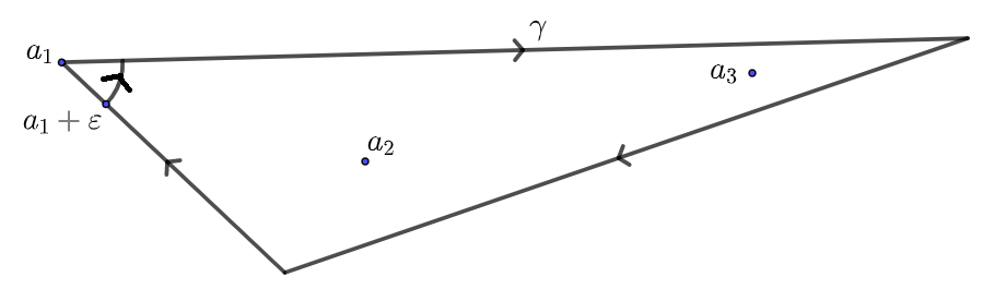
By property (4) of the proposition above, we can translate $S$ by any Mobius $R$, so we can assume WLOG that $\infty\in S$, and end points of $\gamma$ being finite, so $\gamma$ is a path in the finite plane. Let $S-\{\infty\}=\{a_{1},\cdots,a_{k}\}$. $\gamma$ be a path with base point $a_{1}\in S$. Let $I=\int_{\gamma}(\omega(c_{1})-\omega(d_{1}))(\omega(c_{2})-\omega(d_{2}))\cdots(\omega(c_{n})-\omega(d_{n}))$, with $c_{i},d_{i}\in S$, $c_{1},d_{1},c_{n},d_{n}\neq a_{1}$. We need to show $I\in\overline{\textsf{MZV}^{S}_{n}}$. Since $\infty\in S$, we can split the above iterated integral into $2^{n}$ terms, each is then in $\textsf{MZV}^{S}_{n}$, it suffices to prove each of them is in $\overline{\textsf{MZV}^{S}_{n}}$, say $I=\int_{\gamma}\omega(c_{1})\cdots\omega(c_{n})$. Let $X$, the set of alphabets for formal series manipulations below, to be $X=\{\omega(a_{1}),\cdots,\omega(a_{k})\}$.

Firstly, since $c_{1},c_{n}\neq a_{1}$, we can perturb the $\gamma$ by $\varepsilon>0$, say into $\gamma(\varepsilon)$, which is a path based at $a_{1}+\varepsilon$, we will have $\lim_{\varepsilon\to 0}\int_{\gamma(\varepsilon)}\omega(c_{1})\cdots\omega(c_{n})=I$. (See figure 1 for illustration).

Figure 1. Perturbation of the original $\gamma$

Recall the formal series $\mathbb{C}\llangle X\rrangle$ ring defined previously. Now $\gamma$ represents an element of the fundamental group $G=\pi_{1}(\hat{\mathbb{C}}-S,a_{1}+\varepsilon)$, recall we have a homomorphism

$$G\to\mathbb{C}\llangle X\rrangle\qquad\gamma_{1}\mapsto\sum_{\omega\in X^{\ast}}\int_{\gamma_{1}}\omega$$

$G$ is a free group of rank $|S|-1=k$, each generator can be viewed as a loop at $a_{1}+\varepsilon$ and enclosing only $a_{i}$ for each $a_{i}\in S$ (figure 2), say loop $\gamma_{i}(\varepsilon)$. Therefore it suffices to show the corresponding statement with $\lim\int_{\gamma(\varepsilon)}$ replaced by $\lim\int_{\gamma_{i}(\varepsilon)}$.

Figure 2.

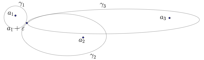
For $\gamma_{1}(\varepsilon)$, it is easy to see that $\lim I_{1}(\varepsilon)=\exp(2\pi i\omega(a_{1}))\in\mathbb{C}\llangle X\rrangle$ (recall that $a_{1}\neq\infty$), whose weight $n$ coefficient ($n\geq 2$) are obviously in $\overline{\textsf{MZV}^{S}_{n}}$. So it remains to prove the claim for the other $\gamma_{i}$. If $a_{i}\notin\{c_{1},\cdots,c_{n}\}$ (i.e. no singularity inside the loop), then $\int_{\gamma_{i}(\varepsilon)}\omega_{1}\cdots\omega_{n}=0$, there is nothing to prove in this case. Therefore assume WLOG that $a_{3}=c_{3}$.

Deform $\gamma_{i}(\varepsilon)$ into following:

thus

$$\textbf{I}_{\gamma_{3}(\varepsilon)}:=\sum_{\omega\in X^{\ast}}\int_{\gamma_{3}(\varepsilon)}\omega=\textbf{I}_{\Gamma_{1}}^{-1}\textbf{I}_{\Gamma_{2}}\textbf{I}_{\Gamma_{1}}$$

now by propositions in previous section, $\lim_{\varepsilon\to 0}\textbf{I}_{\Gamma_{2}}=e^{-2\pi i\omega(a_{3})}$, and

$$\textbf{I}_{\Gamma_{1}}=e^{A_{\varepsilon}\omega(a_{3})}\tilde{\textbf{I}}e^{B_{\varepsilon}\omega(a_{1})}+O(\varepsilon^{1/2})$$

with $\tilde{\textbf{I}}$ the unique group-like lift of $\lim_{\varepsilon\to 0}\pi(\textbf{I}_{\Gamma_{1}})$ with coefficients of $\omega(a_{1}),\omega(a_{3})$ being 0, note that by (2.5), coefficient of it lies in $\textsf{MZV}^{S}_{n}$. Modulo $O(\varepsilon^{1/2})$ and multiple of $2\pi i$,

$$A_{\varepsilon}\equiv\int_{a_{1}+\varepsilon}^{a_{3}-\varepsilon}\frac{1}{x-a_{3}}dx=-\log\varepsilon-\log(a_{3}-a_{1})$$

and similarly one can see $B_{\varepsilon}\equiv-A_{\varepsilon}$. Therefore

$$\textbf{I}_{\gamma_{3}(\varepsilon)} =e^{-B_{\varepsilon}\omega(a_{1})}\tilde{\textbf{I}}^{-1}e^{-A_{\varepsilon}\omega(a_{3})}e^{-2\pi i\omega(a_{3})}e^{A_{\varepsilon}\omega(a_{3})}\tilde{\textbf{I}}e^{B_{\varepsilon}\omega(a_{1})}+O(\varepsilon^{1/2})$$

$$=e^{-B_{\varepsilon}\omega(a_{1})}\tilde{\textbf{I}}^{-1}e^{-2\pi i\omega(a_{3})}\tilde{\textbf{I}}e^{B_{\varepsilon}\omega(a_{1})}+O(\varepsilon^{1/2})$$

Recall our goal is to show $\lim_{\varepsilon\to 0}\int_{\gamma_{3}(\varepsilon)}\omega_{1}\cdots\omega_{n}\in\overline{\textsf{MZV}^{S}_{n}}$, with $\omega_{1},\omega_{n}\neq\omega(a_{1})$. Therefore the rightmost and leftmost terms $e^{B_{\varepsilon}\omega(a_{1})}$ in above can be ignored, therefore modulo $\overline{\textsf{MZV}^{S}_{n}}$ (see 2.3),

$$\lim_{\varepsilon\to 0}\int_{\gamma_{3}(\varepsilon)}\omega_{1}\cdots\omega_{n}\equiv\tilde{\textbf{I}}^{-1}[\omega_{1}\cdots\omega_{n}]+e^{-2\pi i\omega(a_{3})}[\omega_{1}\cdots\omega_{n}]+\tilde{\textbf{I}}[\omega_{1}\cdots\omega_{n}]$$

here $[\omega_{1}\cdots\omega_{n}]$ means the corresponding coefficient, the first and third term cancels, while for second term, it is in $\overline{\textsf{MZV}^{S}_{n}}$ when weight $n\geq 2$. ∎

For our given finite $S$, denote by $G$ its symmetry group, i.e. group of Mobius transformation $R$ such that $R(S)=S$. We will see later that $G$ affects critically the properties of $\textsf{MZV}^{S}_{n}$.

We need the following technical definition:

Definition 3.4.

Let $T=\{(t_{1},s_{1}),\cdots,(t_{r},s_{r})\}$ be a subset of $S^{2}$. We construct an undirected graph, with vertex set $S$ as follows: start with the empty graph (vertex $S$ and no edge), for each $(t_{i},s_{i})\in T$ and each $g\in G$, join vertices $gt_{i}$ and $gs_{i}$ with an edge. Denote this graph by $\mathcal{G}^{S}(T)$.

Definition 3.5.

Let $T=\{(t_{1},s_{1}),\cdots,(t_{r},s_{r})\}$ be a subset of $S^{2}$. We call $T$ a set of complete edges if

• Union of orbits of $t_{i}$, $s_{i}$ covers $S$.

• The graph $\mathcal{G}^{S}(T)$ is connected.

Theorem 3.6.

Let $T=\{(t_{1},s_{1}),\cdots,(t_{r},s_{r})\}$ be a set of complete edges of $S$, choose any path $\gamma_{1},\cdots,\gamma_{r}$, with end points of $\gamma_{i}$ being $t_{i},s_{i}$. In the definition of $\textsf{MZV}^{S}_{n}$, let $V_{n}$ be the vector subspace formed by taking, instead of $\gamma$ over all paths with end points in $S$, now taking $\gamma$ to be only those paths $\gamma_{1},\cdots,\gamma_{r}$. Then $V_{n}\otimes_{\mathbb{Q}}\textsf{MZV}^{S}_{1}=\textsf{MZV}^{S}_{n}$.

Proof.

Note that $V_{n}$ is unchanged if any of $\gamma_{i}$ is replaced by its reverse $\gamma_{i}^{-1}$, so we can enlarge $T$ by adjoining $\{(s_{1},t_{1}),\cdots,(s_{r},t_{r})\}$. As in the start of the previous proof, we can assume $\infty\in S$ and $\gamma$ lies entirely in finite plane, and reduce to show that $\int_{\gamma}\omega(c_{1})\cdots\omega(c_{n})\in V_{n}\otimes_{\mathbb{Q}}(2\pi i)$, where $c_{1}\neq\gamma(1),c_{n}\neq\gamma(0)$. Denote $S-\{\infty\}=\{a_{1},\cdots,a_{k}\}$, $X=\{\omega(a_{1}),\cdots,\omega(a_{k})\}$. We prove the statement by induction on $n$, the case $n=1$ is true since we have already tensored the weight $1$ space, thus we assume $n\geq 2$.

Let $\gamma$ such a path, by definition of $T$ being completed, this implies there exists a chain

$$(g_{1}t_{1},g_{1}s_{1}),(g_{2}t_{2},g_{2}s_{2}),\cdots(g_{q}t_{q},g_{q}s_{q})$$

with $g_{i}s_{i}=g_{i+1}t_{i+1}$, $g_{1}t_{1}=\gamma(0),g_{q}s_{q}=\gamma(1)$. Therefore the path composition $\rho:=\gamma^{-1}(g\gamma_{q})\cdots(g\gamma_{1})$ is a loop based at $\gamma(0)$, by proposition above, $\int_{\rho}\omega(c_{1})\cdots\omega(c_{n})$ is in $\overline{\textsf{MZV}^{S}_{n}}$, which by induction hypothesis, is in $V_{n}\otimes_{\mathbb{Q}}\textsf{MZV}^{S}_{1}$. Therefore it suffices to prove for $\iota:=(g\gamma_{q})\cdots(g\gamma_{1})$, $\int_{\iota}\omega(c_{1})\cdots\omega(c_{n})\in V_{n}\otimes_{\mathbb{Q}}\textsf{MZV}^{S}_{1}$. Of course, $\iota$ can pass through the singularities $S$ of the integrand, so $\int_{\iota}$ does not make sense, but it suffices to prove this for a slight deformation of $\iota$ which does not pass through any points of $S$ ("difference" of any two different deformations is a loop, so is in $V_{n}\otimes_{\mathbb{Q}}\textsf{MZV}^{S}_{1}$).

Consider the following deformation of the path $\iota$, where a circular arc is used to indent singularities.

Here $\gamma_{0,\varepsilon}$ and $\gamma_{1,\varepsilon}$ are slight perturbation of the end point $\gamma(0)$ and $\gamma(1)$ respectively. Denote $\lim$ to be the process when radii of all circular arcs $\to 0$. Let $\textbf{I}_{i}\in\mathbb{C}\llangle X\rrangle$ be the associated element of $g_{i}\gamma_{i}$ as shown in figure, and $\textbf{C}_{i}\in\mathbb{C}\llangle X\rrangle$ be the associated element of circular arcs. Then

$$\textbf{I}_{\gamma_{0,\varepsilon}\to\gamma_{1,\varepsilon}}=\textbf{C}_{q}\textbf{I}_{q}\cdots\textbf{C}_{1}\textbf{I}_{1}\textbf{C}_{0}$$

Let us temporarily assume each $g_{i}s_{i}$ is finite. Taking $\lim$ both sides, each $\textbf{C}_{i}$ tends to $e^{A_{i}\omega(g_{i}s_{i})}$ for $A_{i}\in\mathbb{C}$, and $\textbf{I}_{i}=e^{B_{i,\varepsilon}}\tilde{\textbf{I}}_{i}e^{C_{i,\varepsilon}}+O(\varepsilon)$, here $\tilde{\textbf{I}}_{i}$ is, as always, the unique group-like lift of $\lim\pi_{i}(\textbf{I}_{i})$ with $\pi_{i}$ suitable projection, and the two suitable linear coefficients being $0$. Plug these into the above displayed equation, we obtain, as in argument of the proof of 2.3, with renaming of constants if necessary,

(3.4) $$\textbf{I}_{\gamma_{0,\varepsilon}\to\gamma_{1,\varepsilon}}=e^{B_{\varepsilon}\omega(\gamma(1))}\tilde{\textbf{I}}_{q}e^{A_{q}\omega(g_{q}t_{q})}\tilde{\textbf{I}}_{q-1}e^{A_{q-1}\omega(g_{q-1}t_{q-1})}\cdots\tilde{\textbf{I}}_{2}e^{A_{2}\omega(g_{2}t_{2})}\tilde{\textbf{I}}_{1}e^{C_{\varepsilon}\omega(\gamma(0))}+O(\varepsilon)$$

for some $A_{i}\in\mathbb{C}$.

We claim the coefficient of any weight $n$ word $\omega(d_{1})\cdots\omega(d_{n})$ in $\tilde{\textbf{I}}_{i}$, is actually in $V_{n}$. Indeed, for convergent integral, the coefficient of $\omega(d_{1})\cdots\omega(d_{n})$ in $\tilde{\textbf{I}}_{i}$ is

$$\int_{g\circ\gamma_{i}}\omega(d_{1})\cdots\omega(d_{n})=\int_{\gamma_{i}}g^{\ast}\omega(d_{1})\cdots g^{\ast}\omega(d_{n})$$

because $g^{\ast}\omega(a)=\omega(g^{-1}(a))-\omega(g^{-1}(\infty))$, $g(S)=S$ and $\infty\in S$, the above is in $V_{n}$ (recall definition of $V_{n}$: only those paths $\gamma_{i}$ are allowed). Next, if the coefficient represents an integral that does not converge, by (2.5), this coefficient is a $\mathbb{Q}$-combination of above, so again in $V_{n}$.

Recall our goal is to show coefficient of $\omega\in X^{\ast}$ in $\lim\textbf{I}_{\gamma_{0,\varepsilon}\to\gamma_{1,\varepsilon}}\in\mathbb{C}\llangle X\rrangle$, with $\omega$ not starting in $\omega(\gamma(1))$ and not ending in $\omega(\gamma(0))$, lies in $V_{n}\otimes_{\mathbb{Q}}\textsf{MZV}^{S}_{1}$. For any such coefficient of $\omega\in X^{\ast}$, the two exponentials at the both ends of (3.4) plays no role, so this coefficient $\int_{\iota}\omega$ is simply the coefficient of $\omega$ in

$$\tilde{\textbf{I}}_{q}e^{A_{q}\omega(g_{q}t_{q})}\tilde{\textbf{I}}_{q-1}e^{A_{q-1}\omega(g_{q-1}t_{q-1})}\cdots\tilde{\textbf{I}}_{2}e^{A_{2}\omega(g_{2}t_{2})}\tilde{\textbf{I}}_{1}$$

we just shown coefficients of $\tilde{\textbf{I}}_{i}$ lies in $V_{n}$, it remains to see each $A_{i}\in\textsf{MZV}^{S}_{1}$. Here we can assume $g_{i}t_{i}$ are distinct: if they were not, then we can remove a loop from $\iota$, this loop are have coefficients in already $V_{n}\otimes_{\mathbb{Q}}\textsf{MZV}^{S}_{1}$, so does not affect the result. For each $g_{i}t_{i}$, we have

$$\int_{\iota}\omega(g_{i}t_{i})=A_{i}+\sum_{j}\tilde{\textbf{I}}_{j}[\omega(g_{i}t_{i})]$$

here $\textbf{I}[\omega]$ represent coefficient of corresponding term. Above LHS is in $\textsf{MZV}^{S}_{1}$; while for RHS, $\tilde{\textbf{I}}_{j}[\omega(g_{i}t_{i})]$, if it comes a convergent integral, then it is in $\textsf{MZV}^{S}_{1}$, otherwise by our choice of $\tilde{\textbf{I}}_{j}$, it is $0$, therefore $A_{i}\in\textsf{MZV}^{S}_{1}$. Completing the proof when each of $g_{i}t_{i}$ is finite.

Finally, we need to dispose of the case when one of $g_{i}t_{i}=\infty$. This case is largely parallel to above, by 2.5, one just have to simply replace $e^{A_{i}\omega(g_{i}t_{i})}$ in (3.4) into $e^{A_{i}(\omega(a_{1})+\cdots+\omega(a_{k}))}$, here recall that $\{a_{1},\cdots,a_{k}\}=S-\{\infty\}$. The rest of argument goes through identically. ∎

We record here a spanning set of $\textsf{MZV}^{S}_{1}$. Recall the notion of cross-ratio: for any four $z_{i}\in\hat{\mathbb{C}}$, it is defined to be $\frac{(z_{3}-z_{1})(z_{4}-z_{2})}{(z_{3}-z_{2})(z_{4}-z_{1})}$, it is a Mobius transformation invariant: if $z_{i}$ map to $w_{i}$, then their cross-ratio are the same.

Lemma 3.7.

$2\pi i$, together with the logarithm of cross-ratios of all $4$-tuple of elements in $S$, span $\textsf{MZV}^{S}_{1}$.

Proof.

Essentially follows from the formula

$$\int_{a}^{b}\omega(c)-\omega(d)=\log\frac{(b-c)(a-d)}{(a-c)(b-d)}$$

$2\pi i$ arises from different branch of log. ∎

Since for any Mobius transformation, $\textsf{MZV}^{S}_{n}=\textsf{MZV}^{R(S)}_{n}$, for any $S$ with $|S|\geq 3$, we can assume WLOG that $S$ contains $\{0,1,\infty\}$. Since $\omega(\infty)=0$, by taking all $d_{i}=\infty$ in (3.1), we obtain

Corollary 3.8.

(a) Let $R$ be a Mobius transformation of such that $\{0,1,\infty\}\subset R(S)$. Suppose $\{0,1,\infty\}\subset R(S)$, then

$$\int_{0}^{1}\omega(a_{1})\cdots\omega(a_{n})\in\textsf{MZV}^{S}_{n}$$

for $a_{1}\neq 1,a_{n}\neq 0,a_{i}\in R(S)$.

(b) Let $R$ be a rational function such that $R^{-1}(R(S))\subset S$. Suppose $\{0,1,\infty\}\subset R(S)$ then

$$\int_{0}^{1}\omega(a_{1})\cdots\omega(a_{n})\in\textsf{MZV}^{S}_{n}$$

for $a_{1}\neq 1,a_{n}\neq 0,a_{i}\in R(S)$.

Note that $(a)$ is a special case of $(b)$.

4. Applications to Colored Multiple Zeta Values

Now we apply the material developed in the previous section to CMZV. Recall the space $\textsf{CMZV}^{N}_{w}$ is defined to be $\mathbb{Q}$-span of all

$$\sum_{s_{1}>\cdots>s_{k}\geq 1}\frac{a_{1}^{n_{1}}\cdots a_{k}^{n_{k}}}{n_{1}^{s_{1}}\cdots n_{k}^{s_{k}}}$$

where $a_{i}$ are $N$-th roots of unity, $s_{i}$ are positive integers and $(a_{i},s_{i})\neq(1,1)$. Here $N$ is called level and $w$ weight. By (2.3), $\textsf{CMZV}^{N}_{w}$ is the same as the span of

$$\int_{0}^{1}\omega(a_{1})\cdots\omega(a_{w})$$

with $a_{i}=0$ or $N$-th root of unity, $a_{1}\neq 1,a_{w}\neq 0$.

Fix a positive integer $N$, let $S=\{0,\infty,1,\mu,\cdots,\mu^{N-1}\}$ with $\mu=e^{2\pi i/N}$. The symmetry group $G$ of $S$ is the dihedral group of order $2N$, generated by multiplication of a root of unity $x\mapsto\mu x$ and reflection $x\mapsto 1/x$.

Lemma 4.1.

When $N\geq 3$, $2\pi i\in\textsf{CMZV}^{N}_{1}$.

Proof.

We only weight 1 CMZVs are

$$\sum_{n=1}^{\infty}\frac{\mu^{in}}{n}=-\log(1-\mu^{i})$$

on the other hand

$$\log(1-e^{i\theta})-\log(1-e^{-i\theta})=(\theta-\pi)i\qquad 0<\theta<2\pi$$

therefore when $0<\theta<2\pi$ can be chosen to be $\neq\pi$, $i\pi\in\textsf{CMZV}^{N}_{1}$, this is possible for $N\geq 3$. ∎

Lemma 4.2.

When $N\geq 3$, $\textsf{CMZV}^{N}_{1}=\textsf{MZV}^{S}_{1}$. When $N=1$ or $2$, $\textsf{CMZV}^{N}_{1}$ adjoining $2\pi i$ equals $\textsf{MZV}^{S}_{1}$.

Proof.

The cases for $N=1,2$ are trivial, since both sides can be computed explicitly. We prove the assertion for $N\geq 3$, $\textsf{CMZV}^{S}_{1}\subset\textsf{MZV}^{S}_{1}$ is evident. For the converse inclusion, by lemma 3.7, it suffices to show $\log$ of each $4$-tuple’s cross ratio in $S$, can be written as a linear combination of $2\pi i$ and $\log(1-\mu^{i})$. This is an explicit computation: for example, when the four points are $\mu^{a},\mu^{b},\mu^{c},\mu^{d}$, the cross-ratio is $(1-\mu^{b-a})(1-\mu^{d-c})/(1-\mu^{d-a})(1-\mu^{b-c})$, whose log is obviously a linear combination of $2\pi i$ and $\log(1-\mu^{i})$; similarly, for four points $\{0,1,\infty,\mu^{i}\}$, cross ratio is $1-\mu^{i}$, so this is again true, similarly one can checks all other cases. ∎

Theorem 4.3.

Let $S=\{0,\infty,1,\mu,\cdots,\mu^{N-1}\}$ with $\mu=e^{2\pi i/N}$. For $N\geq 3$, $\textsf{CMZV}^{N}_{w}=\textsf{MZV}^{S}_{w}$. For $N=1$ or $2$, $\textsf{CMZV}^{N}_{w}\otimes_{\mathbb{Q}}\mathbb{Q}[2\pi i]=\textsf{MZV}^{S}_{w}$.

Proof.

First we claim $T=\{(0,1)\}$ is a set of complete edges for $S$. Indeed, starting from $(0,1)$, acting by $x\mapsto\mu^{i}x$ gives $(0,\mu^{i})$. So $\mu^{i}$ are in connected component of the vertex $0$. Taking $x\mapsto 1/x$ gives $(\infty,1)$, so $\infty$ is also in the connected component of vertex $0$, so $\mathcal{G}^{S}(T)$ is connected.

Next we show the space $V_{n}$ defined in 3.6 is simply $\textsf{CMZV}^{N}_{w}$. Indeed, definition of $V_{n}$ is the $\mathbb{Q}$-span of

$$\int_{0}^{1}(\omega(c_{1})-\omega(d_{1}))\cdots(\omega(c_{n})-\omega(d_{n}))$$

for over all $c_{i},d_{i}\in S,c_{1},d_{1}\neq 1,c_{n},d_{n}\neq 0$. By taking each $d_{i}=\infty$, we see that $\textsf{CMZV}^{N}_{n}\subset V_{n}$. Only the other hand, given any $c_{i},d_{i}$ as above, above integral can be expanded into $2^{n}$ terms, each of them in $\textsf{CMZV}^{N}_{n}$, so the two space are equal.

Therefore $\textsf{CMZV}^{N}_{n}\otimes_{\mathbb{Q}}\textsf{MZV}^{S}_{1}=\textsf{MZV}^{S}_{n}$. The claim then follows from the above lemma. ∎

Above theorem actually has some very profound consequences. For example, it follows immediately that from 3.8:

Corollary 4.4.

Let $S=\{0,\infty,1,\mu,\cdots,\mu^{N-1}\}$ with $\mu=e^{2\pi i/N}$ and $N\geq 3$, (a) Let $R$ be a Mobius transformation of such that $\{0,1,\infty\}\subset R(S)$, we have

$$\int_{0}^{1}\omega(a_{1})\cdots\omega(a_{n})\in\textsf{CMZV}^{N}_{n}$$

for $a_{1}\neq 1,a_{n}\neq 0,a_{i}\in R(S)$.

(b) Let $R$ be a rational function such that $R^{-1}(R(S))\subset S$, then

$$\int_{0}^{1}\omega(a_{1})\cdots\omega(a_{n})\in\textsf{CMZV}^{N}_{n}$$

for $a_{1}\neq 1,a_{n}\neq 0,a_{i}\in R(S)$.

4.1. Some qualitative examples

Example 4.5.

Let $N=5,\mu=e^{2\pi i/5}$, let $R$ be the Mobius transform such that $R^{-1}(0)=\mu,R^{-1}(1)=1,R^{-1}(0)=\mu^{2}$, then $R$ maps $S=\{0,\infty,1,\mu,\mu^{2},\mu^{3},\mu^{4}\}$ to

$$\{-\mu-\mu^{2}-\mu^{3},1+\mu,1,0,\infty,\frac{1}{2}\left(\sqrt{5}+3\right),\frac{1}{2}\left(\sqrt{5}+1\right)\}$$

so when $a_{i}$ are finite values in above list, $\int_{0}^{1}\omega(a_{1})\cdots\omega(a_{n})$ when $a_{1}\neq 1,a_{n}\neq 0$ is level 5 CMZV. In particular, using (2.3), we see that, for multiple polylogarithm $\operatorname{Li}_{s_{1},\cdots,s_{n}}(x_{1},\cdots,x_{n})$, if $x_{1}^{-1},x_{1}^{-1}x_{2}^{-1},\cdots,x_{1}^{-1}\cdots x_{n}^{-1}$ is contained in

$$\{-\mu-\mu^{2}-\mu^{3},1+\mu,1,\frac{1}{2}\left(\sqrt{5}+3\right),\frac{1}{2}\left(\sqrt{5}+1\right)\}$$

then $\operatorname{Li}_{s_{1},\cdots,s_{n}}(x_{1},\cdots,x_{n})\in\textsf{CMZV}^{5}_{w}$ with $w=\sum s_{i}$. In particular:

• The generalized polylogarithm $\operatorname{Li}_{s_{1},\cdots,s_{n}}(z)\in\textsf{CMZV}^{5}_{w}$ if $z=(\sqrt{5}-1)/2$ or $(3-\sqrt{5})/2$

• The multiple polylogarithm $\operatorname{Li}_{s_{1},\cdots,s_{n}}(x_{1},\cdots,x_{n})\in\textsf{CMZV}^{5}_{w}$ if $n-2$ of $x_{i}$’s are equal $1$, and the remaining two $=(\sqrt{5}-1)/2$.

these two points are not obvious from the very definition of $\textsf{CMZV}^{5}$, where only roots of unity appears.

Example 4.6.

Let $N=6,\mu=e^{2\pi i/6}$, let $R$ be the Mobius transform such that $R^{-1}(0)=\mu,R^{-1}(1)=1,R^{-1}(0)=\mu^{3}$, then $R$ maps $S=\{0,\infty,1,\mu,\mu^{2},\mu^{3},\mu^{4},\mu^{5}\}$ to

$$\{1-i\sqrt{3},1+i\sqrt{3},1,0,-2,\infty,4,2\}$$

so when $a_{i}$ are finite values in above list, $\int_{0}^{1}\omega(a_{1})\cdots\omega(a_{n})$ when $a_{1}\neq 1,a_{n}\neq 0$ is level 5 CMZV. In particular, using (2.3), we see that, for multiple polylogarithm $\operatorname{Li}_{s_{1},\cdots,s_{n}}(x_{1},\cdots,x_{n})$, if $x_{1}^{-1},x_{1}^{-1}x_{2}^{-1},\cdots,x_{1}^{-1}\cdots x_{n}^{-1}$ is contained in

$$\{1-i\sqrt{3},1+i\sqrt{3},1,-2,4,2\}$$

then $\operatorname{Li}_{s_{1},\cdots,s_{n}}(x_{1},\cdots,x_{n})\in\textsf{CMZV}^{6}_{w}$ with $w=\sum s_{i}$. In particular:

• The generalized polylogarithm $\operatorname{Li}_{s_{1},\cdots,s_{n}}(z)\in\textsf{CMZV}^{6}_{w}$ if $z=1/2,-1/2$ or $1/4$

• The multiple polylogarithm $\operatorname{Li}_{s_{1},\cdots,s_{n}}(x_{1},\cdots,x_{n})\in\textsf{CMZV}^{6}_{w}$ if $n-2$ of $x_{i}$’s are equal $1$, and the remaining two $=1/2$ or $=-1/2$.

Example 4.7.

Let $N=10,\mu=e^{2\pi i/10}$, let $R$ be the Mobius transform such that $R^{-1}(0)=1,R^{-1}(1)=\mu^{2},R^{-1}(0)=\mu^{6}$, then $R$ maps $S=\{0,\infty,1,\mu,\cdots,\mu^{9}\}$ to

$$\left\{\alpha,\bar{\alpha},0,\frac{1}{2},1,\frac{1}{2}\left(\sqrt{5}+1\right),\frac{1}{2}\left(\sqrt{5}+3\right),\sqrt{5}+3,\infty,-\sqrt{5}-2,\frac{1}{2}\left(-\sqrt{5}-1\right),\frac{1}{2}\left(1-\sqrt{5}\right)\right\}$$

here $\alpha=\mu+\mu^{3}$. So when $a_{i}$ are finite values in above list, $\int_{0}^{1}\omega(a_{1})\cdots\omega(a_{n})$ when $a_{1}\neq 1,a_{n}\neq 0$ is level 10 CMZV. In particular, generalized polylogarithm $\operatorname{Li}_{s_{1},\cdots,s_{n}}(z)\in\textsf{CMZV}^{10}_{w}$ if $z=1/(3+\sqrt{5})$ or $1/(-2-\sqrt{5})$.

Note that the number $1/2$ is in above list, which makes the iterated integral $\int_{0}^{1}\omega(a_{1})\cdots\omega(a_{n})$ problematic when one of $a_{i}=1/2$. However, from our proofs of theorems in previous section, the straight-line path $[0,1]$ can actually be replaced by any path with same end-points, and does not affect the qualitative statement $\in\textsf{CMZV}^{10}$.

We introduce the following notion: we call an iterated integral with support $B\subset\mathbb{C}$ is a level $N$ CMZV, if

$$\int_{0}^{1}\omega(b_{1})\cdots\omega(b_{n})\in\textsf{CMZV}^{N}_{n}\qquad\forall b_{i}\in B,b_{1}\neq 1,b_{n}\neq 0\qquad\forall n\geq 1$$

Above example shows iterated integral with support $\{0,1,(\sqrt{5}+1)/2\}$ has level $5$, similarly, one can show support $\{0,1,(-\sqrt{5}+1)/2\}$ has also level $5$. The $N=10$ example then shows when the support is their union: $\{0,1,(\sqrt{5}+1)/2,(-\sqrt{5}+1)/2\}$, the integral has now level $10$.

For general level $N$, $S=\{0,\infty,1,\mu,\cdots,\mu^{N-1}\}$, for each permutation of $\{0,\infty,1\}$, there exists a Mobius transformation $R$ that sends $\{0,\infty,1\}$ to this permutation, therefore, we obtain:

Corollary 4.8.

Assume $0,1\notin B$. If iterated integral with support $B$ has level $N$, then so is those with support $\{0,1\}\sqcup f(B)$, where $f(x)$ can be one of

$$\left\{x,1-x,\frac{1}{x},1-\frac{1}{x},\frac{1}{1-x},-\frac{x}{1-x}\right\}$$

Proof.

The list of 6 functions are Mobius transformation that maps $\{0,\infty,1\}$ to all its permutations, so the result follows from 3.8. ∎

If one put $B=\{\mu,\mu^{2},\cdots,\mu^{N-1}\}$, then above corollary is unable to generate those special values given in above three examples, where we used the versatility to pick a Mobius transformation that maps $\{0,1,\infty\}$ to any 3-tuple of $S$, not just permutations of $\{0,1,\infty\}$.

When the level is low, we do have some interesting results:

Corollary 4.9.

$\operatorname{Li}_{s_{1},\cdots,s_{n}}(1/2)\in\textsf{CMZV}^{2}_{s_{1}+\dots+s_{n}}$, and $\operatorname{Li}_{s_{1},\cdots,s_{n}}((1\pm i)/2)\in\textsf{CMZV}^{4}_{s_{1}+\dots+s_{n}}$

Proof.

For $N=2$, take $B=\{-1\}$; for $N=4$, take $B=\{i,-1,-i\}$, then apply one of those six transformations to $B$. One subtle point for $N=2$ is that 3.6 only guarantees $\operatorname{Li}_{s_{1},\cdots,s_{n}}(1/2)\in\textsf{CMZV}^{2}\otimes_{\mathbb{Q}}\mathbb{Q}[2\pi i]$, but LHS is real, and it is easy to see any real element of RHS must be in $\textsf{CMZV}^{2}$ ∎

For any rational $R$ and finite set $S$, if $R^{-1}(R(S))\subset S$, then we have $\textsf{MZV}^{R(S)}_{n}\subset\textsf{MZV}^{S}_{n}$. In previous examples, we only used the case when $R$ is invertible. Now we construct some higher degree examples.

Let $G$ be the group of Mobius that sends a finite set $S$ to $S$. For each subgroup $H$ of $G$, and $R_{0}$ Mobius, $R=\sum_{\sigma\in H}R_{0}\circ\sigma$ is $H$-invariant, and $\deg R\leq|H|$. Hence if $R$ is not a constant, for $s\in\hat{\mathbb{C}}$, the fibre of $R^{-1}(R(s))$ are exactly $Hs$, counted with multiplicity. In particular, $R$ satisfies $R^{-1}(R(S))\subset S$.

Example 4.10.

Let $N=10,\mu=e^{2\pi i/10},S=\{0,\infty,1,\cdots,\mu^{9}\}$. Take $H=\{x,\mu/x\}\subset G$, let $R=x+\mu/x$, it is invariant under $H$. $R(S)$ has $6$ elements: $\{\infty,R(1),R(\mu^{2}),R(\mu^{3}),R(\mu^{4}),R(\mu^{5})\}$. For each $3$-tuple of this set, choose a Mobius $R_{0}$ that maps this tuple to $(0,1,\infty)$. For example: if $R_{0}(R(\mu),R(\mu^{2}),0)=(0,1,\infty)$, then

$$R_{0}(R(S))=\{\frac{1}{2}\left(-\sqrt{5}-1\right),0,1,\infty,-\sqrt{5}-2,-\sqrt{5}-1\}$$

so iterated integral with support $\{\frac{1}{2}\left(-\sqrt{5}-1\right),-\sqrt{5}-2,-\sqrt{5}-1,0,1\}$ has level 10, this cannot proved by using linear $R$ alone (as in previous examples).

If $R_{0}(R(\mu^{4}),R(\mu^{2}),R(\mu^{3}))=(0,1,\infty)$, then

$$R_{0}(R(S))=\{\frac{1}{2},\frac{1}{4}\left(\sqrt{5}+1\right),1,\infty,0,\frac{1}{4}\left(3-\sqrt{5}\right)\}$$

so iterated integral with support $\{\frac{1}{2},\frac{1}{4}\left(\sqrt{5}+1\right),1,0,\frac{1}{4}\left(3-\sqrt{5}\right)\}$ has level 10

Example 4.11.

Let $N=10,\mu=e^{2\pi i/10},S=\{0,\infty,1,\cdots,\mu^{9}\}$. Take $H=\{x,1/x\}\subset G$, let $R=x+1/x$, it is invariant under $H$. $R(S)$ has $7$ elements: $\{\infty,R(1),R(\mu),\cdots,R(\mu^{5})\}$. For each $3$-tuple of this set, choose a Mobius $R_{0}$ that maps this tuple to $(0,1,\infty)$. For example: if $R_{0}(R(1),R(\mu^{3}),R(\mu))=(0,1,\infty)$, then

$$R_{0}(R(S))=\{\frac{1}{2}\left(3\sqrt{5}-5\right),0,\infty,5\sqrt{5}-10,1,\frac{1}{4}\left(15-5\sqrt{5}\right),4\sqrt{5}-8\}$$

If $R_{1}(R(\mu^{5}),R(\mu^{2}),R(1))=(0,1,\infty)$, then

$$R_{1}(R(S))=\{2\sqrt{5}-5,\infty,5,1,45-20\sqrt{5},9-4\sqrt{5},0\}$$

In particular, the generalized polylogarithm at $z$ is in $\textsf{CMZV}^{10}$, when

$$z=2\sqrt{5}-5,\frac{1}{5},45-20\sqrt{5},9-4\sqrt{5},\frac{1}{4}\left(15-5\sqrt{5}\right),4\sqrt{5}-8$$

We can generate more explicit values, whose iterated integral with these supports are CMZV. However, there aren’t too many of them:

Proposition 4.12.

Let $S$ be any finite set of $\hat{\mathbb{C}}$, the number of possible $R$, with $R$ rational function, satisfying $\{0,1,\infty\}\subset R(S)$ and $R^{-1}(R(S))\subset S$ is finite.

Proof.

We have $R^{-1}(0),R^{-1}(1),R^{-1}(\infty)\subset S$, in other words, the divisors of $R$ and $1-R$ have supports contained in $S$, this is a Diophantine equation known as $S$-unit equation (over function field of genus zero curve), and it is known to have only finite many solutions, all of them have $\deg(R)\leq|S|-2$ ([19]). ∎

4.2. Explicit computations

Examples given in previous sections are qualitative: they assert certain iterated integrals are in $\mathbb{Q}$-spnn of CMZVs, but don’t give explicit representation. Goal of this subsection is to illustrate that every qualitative claim in previous section can be made concrete, meaning one write down an expression for values of iterated integrals in terms of CMZV, i.e., im terms of series

$$\sum_{s_{1}>\cdots>s_{k}\geq 1}\frac{a_{1}^{n_{1}}\cdots a_{k}^{n_{k}}}{n_{1}^{s_{1}}\cdots n_{k}^{s_{k}}}$$

with $a_{i}$ roots of unity. The ability to do this algorithmically has been integrated into the Mathematica package mentioned in Appendix. Here algorithmic details are deliberated eschewed, instead we just toy with simple examples to illustrate the techniques.

Before starting, it would be conducive to extend range of words that can be put into iterated integral, by allowing all words, we do this for integral over $[0,1]$.

Definition 4.13.

Let $a_{1},\cdots,a_{n}\in\mathbb{C}$, let $\gamma$ be a slight perturbation of the usual path from $0$ to $1$ lying on upper-half plane. Then there exists $c,c_{ij}\in\mathbb{C}$ such that

$$\int_{\gamma|[\alpha,\beta]}\omega(a_{1})\cdots\omega(a_{n})=c+\sum_{n\geq i+j\geq 0}c_{ij}\log^{i}\alpha\log^{j}(1-\beta)+o(1)\qquad\alpha\to 0^{-},\beta\to 1^{+}$$

we define $\int_{0}^{1}\omega(a_{1})\cdots\omega(a_{n})$ to be $c$.

Existence of such asymptotic expansion follows from 2.3. For convergent integral (i.e. $a_{1}\neq 1,a_{0}\neq 0$), above value coincide with the familiar value. For $X=\{\omega(a_{1}),\cdots,\omega(a_{n})\}$, define

$$\textbf{I}_{[0,1]}(X):=\sum_{\omega\in X^{\ast}}(\int_{0}^{1}\omega)\omega$$

this is a group-like element of $\mathbb{C}\llangle X\rrangle$.

Example 4.14.

We prove previously that iterated integrals with this support are of level 5 (4.5), there we used the Mobius transformation $R$ which maps $R((\mu,1,\mu^{2}))$ to $(0,1,\infty)$. Now let $X=\{\omega(0),\omega(1),\omega(\mu),\cdots,\omega(\mu^{4})\}$,$S=\{0,\infty,1,\cdots,\mu^{4}\}$. Explicitly, $R(z)=((1+\mu)(\mu-z))/(\mu^{2}-z)$.

$$\int_{\alpha}^{\beta}\omega(a_{1})\cdots\omega(a_{n})=\int_{R^{-1}(\alpha,\beta)}(R^{\ast}\omega(a_{1}))\cdots(R^{\ast}\omega(a_{n}))$$

The support of integrand on RHS are $\{0,1,\mu,\mu^{2},\mu^{3},\mu^{4}\}$. When $\alpha$ close to $0$, $\beta$ close to $1$, the limit of integration are close to $\mu$ and $1$, the path $R^{-1}(\alpha,\beta)$ is a circular arc end points approaching $\mu$ to $1$, which is in turn homotopic to:

1. a straight line from $\mu$ to $0$ with argument $2\pi/5$

2. then a small circular arc around origin that changes argument from $2\pi/5$ to $0$

3. finally straight line from $0$ to $1$

Let $\textbf{L}=e^{A\omega(1)}\tilde{\textbf{I}}_{[0,1]}(X)e^{B\omega(0)}g(\tilde{\textbf{I}}_{[0,1]}(X))^{-1}e^{C\omega(\mu)}$ for some to-be-determined constants $A,B,C\in\mathbb{C}$. Then we have

$$\int_{0}^{1}\omega(a_{1})\cdots\omega(a_{n})=\textbf{L}[R^{\ast}\omega(a_{1})\cdots R^{\ast}\omega(a_{n})]\qquad a_{i}\in R(S)$$

where $g$ is the homomorphism defined by $g(\omega(a))=\omega(a\mu^{-1})$. Here one can treat $g(\tilde{\textbf{I}}_{[0,1]}(X))$ as the element in $\mathbb{C}\llangle X\rrangle$ for iterated integrals from $0$ to $\mu$, its inverse is that of the reverse direction: from $\mu$ to $0$; the exponential term $e^{B\omega(0)}$ of L at middle comes the fact that $\omega(0)\in X$; the term $\tilde{\textbf{I}}_{[0,1]}(X)$ corresponds to path from $0$ to $1$; the two exponential $e^{A\omega(1)},e^{C\omega(\mu)}$ are used to make the group-like element coincide with the definition set forth in above definition, if $\int_{0}^{1}\omega(a_{1})\cdots\omega(a_{n})$ is convergent, then values of $A,C$ are of no relevance.

Now we need to determine values of $A,B,C$, this can be done by comparing linear terms. We have

$$\int_{0}^{1}\omega(R(0)) =\textbf{L}[R^{\ast}\omega(R(0))]$$

$$=\textbf{L}[\omega(0)]-\textbf{L}[\omega(\mu^{2})]$$

$$=B-\tilde{\textbf{I}}_{[0,1]}[\omega(\mu^{2})]-g(\tilde{\textbf{I}}_{[0,1]})^{-1}[\omega(\mu^{2})]$$

$$=B-\int_{0}^{1}\omega(\mu^{2})+\int_{0}^{1}\omega(\mu)$$

so

$$B=\int_{0}^{1}(\omega(R(0))+\omega(\mu^{2})-\omega(\mu))$$

which can be shown to be $-2\pi i/5$, it can also be seen directly since the change of argument on small circular arc is $-2\pi/5$.

As for $C$, we have

$$0=\int_{0}^{1}\omega(0) =\textbf{L}[R^{\ast}\omega(0)]$$

$$=\textbf{L}[\omega(\mu)-\omega(\mu^{2})]$$

$$=C+\tilde{\textbf{I}}_{[0,1]}[\omega(\mu^{2})-\omega(\mu^{2})]-g(\tilde{\textbf{I}}_{[0,1]})^{-1}[\omega(\mu)-\omega(\mu^{2})]$$

$$=C+\int_{0}^{1}2\omega(\mu)-\omega(\mu^{2})$$

so

$$C=-\int_{0}^{1}(2\omega(\mu)-\omega(\mu^{2}))=\frac{3\log(\phi)}{2}-\frac{i\pi}{2}-\frac{\log(5)}{4}$$

similar one can find the value of $B$.

Example 4.15.

Continuing the above example, we find the value of $\int_{0}^{1}\omega(0)\omega(1)\omega(\alpha)$ with $\alpha=(\sqrt{5}+1)/2$. Let L as in previous example, we have

$$\int_{0}^{1}\omega(0)\omega(1)\omega(\alpha) =\textbf{L}[R^{\ast}(\omega(0))R^{\ast}(\omega(1))R^{\ast}(\omega(\alpha))]$$

$$=\textbf{L}[(\omega(\mu)-\omega(\mu^{2}))(\omega(1)-\omega(\mu^{2}))(\omega(\mu^{4})-\omega(\mu^{2}))]$$

now we split it into $8$ terms, so we need to find each $\textbf{L}[\omega(a_{1})\omega(a_{2})\omega(a_{3})]$. Since each coefficient of L are effectively computable as CMZV, so is our original iterated integral. The computation is quite involved, and not quite do-able by hand.

5. $\mathbb{Q}$-relations between CMZVs

As an application to the theory developed above, we will find, for levels $N$ and weights $w$ indicated in 5.2, all $\mathbb{Q}$-linear relations among $\textsf{CMZV}^{N}_{w}$, presupposing certain conjectures (see next section).

In the paper [28], a list of known relations between CMZVs are summarized, most important of them are shuffle, stuffle and distribution. We won’t describe them here, but concentrate on finding the so-called non-standard relation that is largely unknown.

Such relations exists when $N$ has at least two prime factors, or $N=2^{k},k\geq 2$ or $N=3^{k},k\geq 2$. Except for $N=4$ where octahedral symmetry is used [29], it is not clear how to find them.

For given $N,n$, let

$$\overline{\textsf{CMZV}^{N}_{n}}=\sum_{1\leq k<n}\textsf{CMZV}^{N}_{k}\textsf{CMZV}^{N}_{n-k}$$

it is actually more elegant to write certain relations modulo $\overline{\textsf{CMZV}^{N}_{n}}$, with an algorithmically computable part in $\overline{\textsf{CMZV}^{N}_{n}}$.

We introduce new notations for differential forms, which are customary in the subject:

$$x_{0}=\frac{dx}{x}=\omega(0),x_{1}=\frac{dx}{1-x}$$

$$a=\frac{dx}{x}\qquad b_{i}=\frac{dx}{\mu^{-i}-x}\qquad\mu=e^{2\pi i/N}$$

5.1. Nonstandard relations: unital functions

There are two sources of new relations. For the first one, we require the following notion, let $S=\{0,\infty,1,\mu,\cdots,\mu^{N-1}\}$,

Definition 5.1.

A rational function $\hat{\mathbb{C}}\to\hat{\mathbb{C}}$ is called $N$-unital if $R^{-1}(0),R^{-1}(1),R^{-1}(\infty)\subset S$.

The number of $N$-unital functions are finite, and they all have $\deg\leq N$. ([9], [19]). Therefore we can in principal find all unital functions for given $N$, we assume this has been done.

Assume we have $N$-unital functions: $R_{1},\cdots,R_{n}$, with $R_{i}(1)=R_{i+1}(0)$, consider

$$\mathbf{PATH}_{R}:=\sum_{\omega\in\{x_{0},x_{1}\}^{\ast}}(\int\omega)\omega$$

here the path of integration are the composite path $R_{1},R_{2},\cdots,R_{n}$, then $\mathbf{PATH}_{R}=\textbf{I}_{R_{1}}\cdots\textbf{I}_{R_{n}}$ where

$$\textbf{I}_{R_{i}}:=\sum_{\omega\in\{x_{0},x_{1}\}^{\ast}}(\int_{0}^{1}R_{i}^{\ast}\omega)\omega$$

the above assume all ends points of $R_{i}$ are distinct from $0,1,\infty$, if some are equal to these, then one has to insert $e^{Ax_{0}}$, or $e^{Ax_{1}}$ or $e^{A(x_{0}-x_{1})}$ respectively between $\textbf{I}_{R_{i}},\textbf{I}_{R_{i+1}}$ such that $R_{i}(1)=R_{i+1}\in\{0,1,\infty\}$; and $\textbf{I}_{R_{i}},\textbf{I}_{R_{i+1}}$ becomes certain regularization (group-like lift) of original integral, with $A$ depends these choices of regularizations. Under the hypothesis $R_{i}$ are $N$-unital, coefficients of $\mathbf{PATH}_{R}$ are in $\textsf{CMZV}^{N}$.

If we have another chain of $N$-unital functions, $T_{1},\cdots,T_{r}$, with $T_{i}(1)=T_{i+1}(0)$, then we can construct as above $\mathbf{PATH}_{T}$. If $T_{1}(0)=R_{1}(0),T_{r}(1)=R_{n}(1)$, then the composite path determined by $R$ and $T$ differ by a loop, so by 3.3, we have

$$\int_{0}^{1}R_{n}^{\ast}\omega+\cdots+R_{n}^{\ast}\omega\equiv\int_{0}^{1}T_{1}^{\ast}\omega+\cdots+T_{r}^{\ast}\omega\pmod{\overline{\textsf{CMZV}^{N}_{n}}}$$

for a homogenous degree $n$ $\omega$.

Example 5.2.

Let $N=6,\mu=e^{2\pi i/6}$,

$$R_{1}=\frac{(1-i\sqrt{3})x}{2(x-\mu^{2})^{2}}\qquad T_{1}=\frac{x^{2}}{1+x+x^{2}}$$

then $R_{1},T_{1}$ are $6$-unital, and both starts at $0$ and ends at $1/3$.

with

$$R_{1}^{\ast}x_{0}=a+2b_{4}\qquad R_{1}^{\ast}x_{1}=b_{3}-2b_{4}+b_{5}$$

$$T_{1}^{\ast}x_{1}=2a+b_{2}+b_{4}\qquad R_{1}^{\ast}x_{1}=-b_{2}+b_{3}-b_{4}$$

therefore $\int_{0}^{1}R_{1}^{\ast}\omega=\int_{0}^{1}T_{1}^{\ast}\omega$ if $\omega$ does not ends in $x_{0}$, for example, letting $\omega=x_{0}x_{0}x_{1}$ yields the relation $\int_{0}^{1}u=0$ with

$$u=4aab_{2}-3aab_{3}+2aab_{4}+aab_{5}+2ab_{2}b_{2}-2ab_{2}b_{3}+2ab_{2}b_{4}+2ab_{4}b_{2}-2ab_{4}b_{4}+2ab_{4}b_{5}+2b_{2}ab_{2}-2b_{2}ab_{3}\\ +2b_{2}ab_{4}+2b_{4}ab_{2}-2b_{4}ab_{4}+2b_{4}ab_{5}+b_{2}b_{2}b_{2}-b_{2}b_{2}b_{3}+b_{2}b_{2}b_{4}+b_{2}b_{4}b_{2}-b_{2}b_{4}b_{3}+b_{2}b_{4}b_{4}\\ +b_{4}b_{2}b_{2}-b_{4}b_{2}b_{3}+b_{4}b_{2}b_{4}+b_{4}b_{4}b_{2}+3b_{4}b_{4}b_{3}-7b_{4}b_{4}b_{4}+4b_{4}b_{4}b_{5}$$

using (2.3) one then obtains a relation of level 6 weight 3 CMZV, which cannot be generated by standard relations.

Putting $\omega$ to be other words generates other independent relations. For weight $3$, this can give $3$ independent non-standard relations.

Although this method gives nonstandard relation, each two chains $R_{1},\cdots,R_{n}$ and $T_{1},\cdots,T_{n}$ gives only a few new relations (this number increases with weight). Fortunately, we have plenty of unital functions, so above scenario abounds.

Example 5.3.

Let $N=6,\mu=e^{2\pi i/6}$. Let

$$R_{1}=\frac{1-\mu^{2}x}{1+x}\qquad T_{1}=\frac{2\left(x-\mu^{2}\right)\left(x-\mu^{5}\right)}{\left(1+i\sqrt{3}\right)(x+1)}$$

with

$$R_{1}^{\ast}(x_{0},x_{1})=(b_{3}-b_{2},-a-b_{3})\qquad T_{1}^{\ast}(x_{0},x_{1})=(-b_{1}+b_{3}-b_{4},-a-b_{3}+b_{5})$$

therefore $\int_{0}^{1}R_{1}^{\ast}\omega=\int_{0}^{1}T_{1}^{\ast}\omega$ if $\omega$ does not ends in $x_{1}$. Let $\omega$ to be some weight $n$ words will yield new nonstandard relation, independent to the one from previous examples.

Example 5.4.

Let $N=8,\mu=e^{2\pi i/8}$. Let $R_{1},R_{2},T_{1},T_{2}$ be such that

$$R_{1}^{\ast}(x_{0},x_{1})=(-a-b_{6},a+b_{5})\qquad R_{2}^{\ast}(x_{0},x_{1})=(b_{2}+b_{3}-2b_{5},-b_{2}-b_{3}+b_{4}+b_{7})$$

$$T_{2}^{\ast}(x_{0},x_{1})=(-a-b_{6},a+b_{7})\qquad T_{1}^{\ast}(x_{0},x_{1})=(-b_{5}+b_{6},b_{4}-b_{6})$$

then $R_{1}(0)=T_{1}(0)=\infty$ and $R_{2}(1)=T_{2}(1)\neq 0$ or $1$, so

We have

(5.1) $$\textbf{I}_{R_{2}}\textbf{I}_{R_{1}}e^{A(x_{0}-x_{1})}=\textbf{I}_{T_{2}}\textbf{I}_{T_{1}}$$

for some constant $A$, where

$$\textbf{I}_{R}:=\sum_{\omega\in\{x_{0},x_{1}\}^{\ast}}(\int_{0}^{1}R^{\ast}\omega)\omega$$

if an integral at a coefficient does not converge, it has to be calculated according to (2.5). Comparing linear terms, it can be shown that $A=-3\pi i/4$. Then for any homogeneous word in $x_{0},x_{1}$, comparing its coefficient on both sides of (5.1) will give relations between level $8$ CMZVs.

For a given weight and level, one can continue to produces until Deligne’s bound has been reached. Generally, one must use many choices of $R_{1},\cdots,R_{n}$ and $T_{1},\cdots,T_{n}$, the two level $6$ examples given above are far from enough.

Deligne’s bound can be reached with above method for the following nonstand levels and weights

• Level $6$, weight $\leq 5$

• Level $8$, weight $\leq 4$

• Level $10$, weight $\leq 3$

• Level $12$, weight $\leq 3$

The above method has been tried on level $10$ and weight $4$, and produces around $70$ nonstandard relations, albeit still $2$ relations away from Deligne’s bound.

Also tried is level 9 weight 3, where $3$ nonstandard relations should be there, the above method cannot produce new relation at all in this case.

5.2. Selected basis of $\textsf{CMZV}^{N}_{w}$

Let $d(w,N)$ be the dimension of $\textsf{CMZV}^{N}_{w}$, a deep result due to Deligne and Goncharov [15] provides an upper bound of $d(w,N)$:

Theorem 5.5.

Let $D(w,N)$ be defined by

$$1+\sum_{w=1}^{\infty}D(w,N)t^{w}=\begin{cases}(1-t^{2}-t^{3})^{-1}\qquad&\text{ if }N=1\\ (1-t-t^{2})^{-1}\qquad&\text{ if }N=2\\ (1-at+bt^{2})^{-1}\qquad&\text{ if }N\geq 3\end{cases}$$

where $a=\varphi(N)/2+\nu(N),b=\nu(N)-1$. Here $v(N)$ denote number of distinct prime factors of $N$ and $\varphi$ is the Euler totient function. Then $d(w,N)\leq D(w,N)$.

The above upper bound are conjectured to be tight except when $N$ is a prime power $p^{n},n\geq 1,p\geq 5$ (for $N=1,2,3,4,8$, a motivic basis of the same dimension is exhibited in [14], for other such $N$, this has been conjectured in [28], although this case is less substantiated). When $N=p^{n},n\geq 1,p\geq 5$, the bound is known to be not tight, nonetheless all $\mathbb{Q}$-relations of CMZVs arise conjecturally via known relations (shuffle, stuffle and distribution relations) [28].

In order to do explicit computations, we need an explicit basis for low weight and lower level CMZVs. For each level $N$ and weight $w$, we will choose ad hoc a set finite $\mathcal{B}_{N,w}$.

The $\mathcal{B}_{N,w}$ will satisfy the following:

• $\mathbb{Q}$-span of $\mathcal{B}_{N,w}$ is $\textsf{CMZV}^{N}_{w}$.

• For $w_{1}+w_{2}=w$, if $a\in\mathcal{B}_{N,w_{1}},b\in\mathcal{B}_{N,w_{2}}$, then there exists $r\in\mathbb{Q}^{\times}$ such that $abr\in\mathcal{B}_{N,w}$

• If $M\mid N$, then $\mathcal{B}_{M,w}\subset\mathcal{B}_{N,w}$

moreover, $\mathcal{B}_{N,w}$ is, conditioned on the truth of aforementioned conjectures, a $\mathbb{Q}$-basis of $\textsf{CMZV}^{N}_{w}$.

For example,

$$\mathcal{B}_{2,1}=\left\{\log 2\right\}\qquad\mathcal{B}_{2,2}=\left\{\pi^{2},\log^{2}(2)\right\}\qquad\mathcal{B}_{2,3}=\left\{\zeta(3),\pi^{2}\log(2),\log^{3}(2)\right\}$$

$$\mathcal{B}_{2,4}=\left\{\text{Li}_{4}\left(\frac{1}{2}\right),\zeta(3)\log(2),\pi^{4},\pi^{2}\log^{2}(2),\log^{4}(2)\right\}$$

$$\mathcal{B}_{3,1}=\{i\pi,\log 3\}\qquad\mathcal{B}_{3,2}=\left\{i\sqrt{3}L_{3,2}(2),\pi^{2},i\pi\log(3),\log^{2}(3)\right\}$$

$$\mathcal{B}_{3,3}=\left\{\zeta(3),i\Im\left(\text{Li}_{3}\left(\frac{1}{2}+\frac{i}{2\sqrt{3}}\right)\right),\sqrt{3}\pi L_{3,2}(2),i\sqrt{3}L_{3,2}(2)\log(3),i\pi^{3},\pi^{2}\log(3),i\pi\log^{2}(3),\log^{3}(3)\right\}$$

here $L_{3,2}(s)$ is the primitive Dirichlet-L function of modulus $3$. For instances, the following level $2$ CMZVs,

$$\operatorname{Li}_{1,1,1}(-1,-1,1)=-\frac{7\zeta(3)}{8}-\frac{1}{6}\log^{3}(2)+\frac{1}{12}\pi^{2}\log(2)$$

$$\operatorname{Li}_{2,1,1}(1,1,-1)=-\text{Li}_{4}\left(\frac{1}{2}\right)-\frac{7}{8}\zeta(3)\log(2)+\frac{\pi^{4}}{80}-\frac{1}{24}\log^{4}(2)-\frac{1}{12}\pi^{2}\log^{2}(2)$$

one sees that RHS are indeed $\mathbb{Q}$-combination of the prescribed elements. For a level $3$ example, $\mu=e^{2\pi i/3}$,

$$\operatorname{Li}_{1,1,1}(\mu^{2},\mu,\mu)=\frac{\pi L_{3,2}(2)}{2\sqrt{3}}+\frac{i\sqrt{3}}{4}L_{3,2}(2)\log(3)-\frac{2\zeta(3)}{3}-\frac{5i\pi^{3}}{432}-\frac{1}{48}\log^{3}(3)-\frac{1}{48}i\pi\log^{2}(3)+\frac{5}{144}\pi^{2}\log(3)$$

For the following value of $(N,w)$, the author has

• An explicit representation of $\mathcal{B}_{N,w}$

• Expression of each CMZV of level $N$ and weight $w$ as a rational combination of elements in $\mathcal{B}_{N,w}$.

These $(N,w)$ are:

• $w\leq 14$ for level 1

• $w\leq 8$ for level 2

• $w\leq 5$ for level 3

• $w\leq 6$ for level 4

• $w\leq 4$ for level 5

• $w\leq 5$ for level 6

• $w\leq 4$ for level 8

• $w\leq 3$ for level 7,10,12

The result of level 1 and 2 are already covered in MZVDatamine [4], though different basis are chosen there.

Most of $\mathcal{B}_{N,w}$ is too long to display here, interested reader should consult the appendix, $\mathcal{B}_{N,w}$ are stored in a Mathematica package introduced therein.

5.3. $\textsf{MZV}^{S}_{n}$ for general $S$

The section advocates author’s opinion that CMZVs is nothing special among $\textsf{MZV}^{S}$ for general $S$.

The theory developed in previous section are valid for any finite set $S$. The case of CMZV specializes to $S=\{0,\infty,1,\mu,\cdots,\mu^{N-1}\}$; and we saw in 4.11 that the symmetry $G$ plays an important role, and $G$ has only a few possibilities.

There are some other configuration of $S$ which are highly symmetric:

	$|S|$	$G$	$\textsf{MZV}^{S}$
Tetrahedron vertices/face centers	4	$A_{4}$	a subspace of $\textsf{CMZV}^{6}$
Tetrahedron edge midpoints	6		$=\textsf{CMZV}^{4}$
Octahedron vertices	6	$S_{4}$	$=\textsf{CMZV}^{4}$
Octahedron face centers	8
Octahedron edge midpoints	12
Icosahedron vertex	12	$A_{5}$
Icosahedron face centers	20
Icosahedron edge midpoints	30

It would be natural to ask about

• $\dim_{\mathbb{Q}}\textsf{MZV}^{S}_{n}$ for each of $S$ above

• How to find all $\mathbb{Q}$-relations between $\textsf{MZV}^{S}_{n}$.

For all of the cases listed above, assume $\{0,1,\infty\}\in S$, then $\textsf{MZV}^{S}_{n}=V_{n}\otimes_{\mathbb{Q}}\textsf{MZV}^{S}_{1}$, with $V_{n}$ span of $\int_{0}^{1}\omega(a_{1})\cdots\omega(a_{n})$ over all $a_{i}\in S,a_{n}\neq 0,a_{1}\neq 1$, this follows from 3.6. We will do a short investigation of icosahedral-vertices case in 6.13.

The shuffle relation generalizes verbatim to $\textsf{MZV}^{S}_{n}$. On the other hand, the parallel of stuffle relation is not immediate; in fact, in case of general $S$, for each cyclic subgroup of $G$, up to conjugation, there is a version of stuffle algebra, form which stuffle relations can be deduced. The usual stuffle algebra of CMZV corresponding to the cyclic subgroup $\{1,\mu,\cdots,\mu^{N-1}\}$ of $G$, with $G$ being dihedral of order $2N$. More about this might appear in a later article.

6. Polylogarithm identities

6.1. Special values of multiple polylogarithm

One of the most immediate consequence of our developed materials are the ability to convert multiple polylogarithm into CMZVs.

Let $N\geq 3$ be positive integer, $S=\{0,\infty,1,\cdots,\mu^{N-1}\}$, the following result follows easily from results in 3.8.

Proposition 6.1.

Let $R$ be a rational function with $R^{-1}(R(S))\subset S$, then for any finite $z\in R(S)$,

$$\operatorname{Li}_{s_{1},\cdots,s_{n}}(z)\in\textsf{CMZV}^{N}_{s_{1}+\cdots+s_{n}}$$

there we used example with $\deg R=1$ or $2$, from which we can already generate multitude of different $z$, this number grows polynomially in $N$. A sample of such $z$’s:

Level	$z$
4	$\frac{1+i}{2}$
5	$\frac{1}{2}\left(1-\sqrt{5}\right),\frac{1}{2}\left(\sqrt{5}-1\right),\frac{1}{2}\left(3-\sqrt{5}\right),\frac{1}{5}(2-\mu+\mu^{2}-2\mu^{3})$
6	$\frac{1}{4},\frac{1}{3},-\frac{1}{2},-\frac{1}{3},\frac{8}{9},\frac{1}{9},-\frac{1}{8},\frac{1}{6}\left(3+i\sqrt{3}\right),-\frac{i}{\sqrt{3}},\frac{1}{4}\left(1-i\sqrt{3}\right)$
7	$\frac{1}{2}\csc\left(\frac{3\pi}{14}\right),\frac{1}{4}\csc^{2}\left(\frac{3\pi}{14}\right),\sin^{2}\left(\frac{\pi}{7}\right)\sec^{2}\left(\frac{\pi}{14}\right),\sin\left(\frac{\pi}{7}\right)\sec\left(\frac{3\pi}{14}\right)$
8	$\frac{1}{4}\left(2-\sqrt{2}\right),\frac{1}{2}\left(2-\sqrt{2}\right),3-2\sqrt{2},-\frac{1}{\sqrt{2}},\frac{1}{8}\left(4-3\sqrt{2}\right),12\sqrt{2}-16,\left(1-\sqrt{2}\right)i$
10	$\frac{1}{5},\sqrt{5}-2,\frac{1}{4}\left(\sqrt{5}+1\right),9-4\sqrt{5},\frac{2}{\sqrt{5}},5\sqrt{5}+11,20\sqrt{5}-44,\frac{1}{16}\left(5-5\sqrt{5}\right),\frac{1}{5}\left(9-4\sqrt{5}\right)$
12	$-\frac{1}{\sqrt{3}},1-\sqrt{3},21-12\sqrt{3},\frac{1}{8}\left(3-3\sqrt{3}\right),\frac{1}{24}\left(12-7\sqrt{3}\right),\frac{1}{18}\left(9-5\sqrt{3}\right),27-15\sqrt{3},97-56\sqrt{3}$

Table 1. Some selected $z$’s for which $\operatorname{Li}(z)\in\textsf{CMZV}^{N}$

Since all putative $\mathbb{Q}$-relations of CMZVs are known, we can check in principal every purported equality where both sides are CMZVs.

Example 6.2.

The following three "closed-form" evaluation of dilogarithm and trilogarithm:

$$\text{Li}_{2}(\frac{1}{2}\left(\sqrt{5}-1\right))=\frac{\pi^{2}}{10}-\log^{2}(\phi)\qquad\text{Li}_{2}(\frac{1}{2}\left(3-\sqrt{5}\right))=\frac{\pi^{2}}{15}-\log^{2}(\phi)$$

$$\text{Li}_{3}(\frac{1}{2}\left(3-\sqrt{5}\right))=\frac{4\zeta(3)}{5}+\frac{2\log^{3}(\phi)}{3}-\frac{2}{15}\pi^{2}\log(\phi)$$

are now easily checked since both sides are CMZV of level $5$.

Example 6.3.

We also have multiple polylogarithm analogue, $\rho=(\sqrt{5}-1)/2$:

$$\operatorname{Li}_{1,1,1,1}(\rho,1,1,\rho)=2\text{Li}_{3}(\rho)\log(\phi)-\frac{1}{4}\text{Li}_{4}(\rho^{2})+2\text{Li}_{4}(\rho)-\frac{2}{5}\zeta(3)\log(\phi)+\frac{5\log^{4}(\phi)}{8}+\frac{7}{60}\pi^{2}\log^{2}(\phi)-\frac{7\pi^{4}}{360}$$

$$\operatorname{Li}_{2,2}(\frac{1}{2},2)=\sum_{n=1}^{\infty}\frac{1}{n^{2}2^{n}}\sum_{m=1}^{n-1}\frac{2^{m}}{m^{2}}=-3\text{Li}_{4}\left(\frac{1}{2}\right)+\frac{7\pi^{4}}{288}-\frac{1}{8}\log^{4}(2)-\frac{1}{8}\pi^{2}\log^{2}(2)$$

Example 6.4.

The following three dilogarithm ladders due to Coxeter [13] are classical:

$$\text{Li}_{2}\left(\rho^{6}\right) =4\text{Li}_{2}\left(\rho^{3}\right)+3\text{Li}_{2}\left(\rho^{2}\right)-6\text{Li}_{2}(\rho)+\frac{7\pi^{2}}{30}$$

$$\text{Li}_{2}\left(\rho^{12}\right) =2\text{Li}_{2}\left(\rho^{6}\right)+3\text{Li}_{2}\left(\rho^{4}\right)+4\text{Li}_{2}\left(\rho^{3}\right)-6\text{Li}_{2}\left(\rho^{2}\right)+\frac{\pi^{2}}{10}$$

$$\text{Li}_{2}\left(\rho^{20}\right) =2\text{Li}_{2}\left(\rho^{10}\right)+15\text{Li}_{2}\left(\rho^{4}\right)-10\text{Li}_{2}\left(\rho^{2}\right)+\frac{\pi^{2}}{5}$$

with $\rho=\phi^{-1}=(\sqrt{5}-1)/2$. The first one has both sides level 10 CMZV, so is now routinely verified. We will prove the last one later this section 6.13. The middle one remains more elusive, but similar techniques might work, see remark at the end of this subsection. We also have the following ladders, where both sides are CMZVs of level 10.

$$\text{Li}_{3}(\rho^{6})-8\text{Li}_{3}(\rho^{3})-6\text{Li}_{3}(\rho)=\frac{3\zeta(3)}{5}-4\log^{3}(\phi)+\frac{2}{5}\pi^{2}\log(\phi)$$

$$36\text{Li}_{4}(\rho)-\frac{9\text{Li}_{4}(\rho^{2})}{4}-16\text{Li}_{4}(\rho^{3})+\text{Li}_{4}(\rho^{6})=\frac{27\log^{4}(\phi)}{4}-\frac{3}{2}\pi^{2}\log^{2}(\phi)+\frac{2\pi^{4}}{9}$$

above two identities have been hinted in page 44 of [18], via classical ladder techniques.

Example 6.5.

The following dilogarithm identity is discovered by Watson in 1937 [25]:

$$\operatorname{Li}_{2}(\alpha)-\operatorname{Li}_{2}(\alpha^{2})=\frac{\pi^{2}}{42}+\log^{2}\alpha\qquad\alpha=\frac{1}{2}\sec\frac{2\pi}{7}$$

this is can also be done with our approach since both sides have level $7$.

Example 6.6.

The following entries are recorded in Ramanujan’s notebooks:

$$\operatorname{Li}_{2}(\frac{1}{3})-\frac{1}{6}\operatorname{Li}_{2}(\frac{1}{9})=\frac{\pi^{2}}{18}-\frac{\log^{2}3}{6}\qquad\operatorname{Li}_{2}(-\frac{1}{2})+\frac{1}{6}\operatorname{Li}_{2}(\frac{1}{9})=\frac{\pi^{2}}{18}+\log 2\log 3-\frac{\log^{2}2}{2}-\frac{\log^{2}3}{3}$$

on which our techniques can be applied since all quantities are in $\textsf{CMZV}^{6}_{2}$.

Conjecture 6.7.

For positive integer $n\geq 1$, we have

$$\operatorname{Li}_{n}(\frac{1+i}{2})+\operatorname{Li}_{n}(\frac{1-i}{2})\in\textsf{CMZV}^{2}_{n}$$

This has been verified for $n\leq 6$, even these cases are only solved after mindlessly solving for all level $4$ weight $n$ CMZVs, whose number grows exponentially. Numerical evidence exists for $n=7$.

Conjecture 6.8.

For positive integer $n\geq 1$, $\rho=(\sqrt{5}-1)/2$, we have

$$\operatorname{Li}_{n}(\rho^{3})-\operatorname{Li}_{n}(-\rho^{3})\in\textsf{CMZV}^{5}_{n}$$

Note that both terms $\operatorname{Li}_{n}(\pm\rho^{3})$ are in $\textsf{CMZV}^{10}_{n}$. So this statement has the same spirit as above, where sums of higher level CMZV reduce to a lower level one. This has been verified for $n\leq 4$. Both conjectures fail if one replace $\operatorname{Li}_{n}$ into its generalized counterpart $\operatorname{Li}_{s_{1},\cdots,s_{n}}$.

Example 6.9.

The following ladders involving powers of $-1/2$, are amendable to our approach they’re level $6$ of weight $4$ and $5$ respectively:

$$\operatorname{Li}_{4}(\frac{-1}{8})=-12\text{Li}_{4}\left(\frac{1}{2}\right)+\frac{27\text{Li}_{4}\left(\frac{1}{4}\right)}{4}+\frac{\pi^{4}}{18}+\frac{5\log^{4}(2)}{8}-\frac{1}{4}\pi^{2}\log^{2}(2)$$

$$\operatorname{Li}_{5}(\frac{-1}{8})=-36\text{Li}_{5}\left(\frac{1}{2}\right)+\frac{81\text{Li}_{5}\left(\frac{1}{4}\right)}{8}+\frac{403\zeta(5)}{16}-\frac{1}{8}3\log^{5}(2)+\frac{1}{4}\pi^{2}\log^{3}(2)-\frac{1}{6}\pi^{4}\log(2)$$

The corresponding generalization for weight $6$ has been conjectured in [10],

(6.1) $$\zeta(5,\bar{1})=\frac{36\text{Li}_{6}\left(\frac{1}{2}\right)}{13}-\frac{81\text{Li}_{6}\left(\frac{1}{4}\right)}{208}+\frac{\text{Li}_{6}\left(-\frac{1}{8}\right)}{39}\\ +\frac{3\zeta(3)^{2}}{8}+\frac{31}{16}\zeta(5)\log(2)-\frac{1787\pi^{6}}{589680}-\frac{1}{208}\log^{6}(2)+\frac{1}{208}\pi^{2}\log^{4}(2)-\frac{1}{156}\pi^{4}\log^{2}(2)$$

here $\zeta(5,\bar{1})=\sum_{i>j}\frac{(-1)^{j}}{i^{5}j}\in\textsf{CMZV}^{2}_{6}$. The only part that is conjectural in above expression is the coefficient of $\pi^{6}$. Had CMZVs of weight 6 level 6 been solved, the identity could be checked mechanically just like those above, however, enormous amount of computation would be necessary.

Numerically, an extension of above for weight $7$ also exists, one could also formulates a parallel to conjecture 6.7 in this case.

The conjectural cases for weight $7$ in this example, together with conjecture 6.7, would imply a order $7$ ladder in [8].

For level $N$ CMZV, the possible $z$’s in 6.1 all satisfy the following: both $z$ and $1-z$ are of the form

$$\mu^{i}\prod_{j}(1-\mu^{a_{j}})^{b_{j}}$$

for integers $i,a_{i},b_{i}$, which can be readily seen by looking at $\operatorname{Li}_{1}(z)=-\log(1-z)$ and $\operatorname{Li}_{1}(1-z)=-\log z$.

In particular, for such $z$, both $z$ and $1-z$ are $S$-units in cyclotomic field $\mathbb{Q}(e^{2\pi i/N})$, with $S$ set of prime ideals lying over prime divisors of $N$. These are solutions to the $S$-unit equation, which there are only finitely many solutions [22], and when $N$ is small, these two set seems to coincide. When $N=10$, there exist $S$-units which seems not to be deducible from 6.1: $-\rho^{10},-\rho^{6}$, we will explain the first one when we prove Coxeter’s third ladder in 6.13.

6.2. Icosahedral MZVs and Coxeter’s ladder

In this section, let $\mathcal{I}$ be 12 vertices of a regular icosahedron, we will investigate the space $\textsf{MZV}^{\mathcal{I}}$ and prove Coxeter’s third ladder. Because for $\mathcal{I}$ under any mobius transformation, $\textsf{MZV}^{\mathcal{I}}$ is the same (3.2), we can pick any model for $\mathcal{I}$, in particular, we let

$$\mathcal{I}=\{0,\infty,\rho\mu^{i},-\rho^{-1}\mu^{i}\}\qquad i=0,1,2,3,4\qquad\rho=\frac{\sqrt{5}-1}{2}\qquad\mu=e^{2\pi i/5}$$

(be aware that $1\notin\mathcal{I}$). Let $G\cong A_{5}$ be the group of mobius transformation that permutes $\mathcal{I}$.

Lemma 6.10.

We have $\operatorname{Li}_{s_{1},\cdots,s_{n}}(-\rho^{10})\in\textsf{MZV}^{\mathcal{I}}_{s_{1},\cdots,s_{n}}$.

Proof.

Let $R(z)=z^{5}$, since $\mathcal{I}$ is invariant under multiplication by $e^{2\pi i/5}$, we have $R^{-1}(R(\mathcal{I}))\subset\mathcal{I}$, therefore (3.2) implies for $R(\mathcal{I})=S=\{0,\infty,\rho^{5},-\rho^{-5}\}$, $\textsf{MZV}^{S}_{n}\subset\textsf{MZV}^{\mathcal{I}}_{n}$. We can replace $S$, after dividing $-\rho^{-5}$ (again by Mobius invariance), by $S=\{0,\infty,1,-\rho^{10}\}$, we still have $\textsf{MZV}^{S}_{n}\subset\textsf{MZV}^{\mathcal{I}}_{n}$. The proof is completed after noting that, for any complex $z$, $\textsf{MZV}^{\{0,1,\infty,z\}}$ contains all generalized polylogarithms at $z$. ∎

Lemma 6.11.

Weight $1$ space $\textsf{MZV}^{\mathcal{I}}_{1}$ has a $\mathbb{Q}$-basis $\{2\pi i,\log 5,\log\rho\}$

Proof.

Follows by computing cross-rations of $4$-tuples in $\mathcal{I}$ and 3.7. ∎

For any two distinct vertex $t,u$, from geometric interpretation of action of $G$ on $\mathcal{I}$, it is easy to see $\{(t,u)\}$ is a set of complete edge. Therefore by 3.6.

Theorem 6.12.

Weight $2$ icosahedral MZVs is a subspace of CMZV of level 10, that is,

$$\textsf{MZV}^{\mathcal{I}}_{2}\subset\textsf{CMZV}^{10}_{2}$$

Proof.

Fix a mobius $R$ such that $0,1,\infty\in R(\mathcal{I})$, taking $t=0,u=1$, 3.6 says $\textsf{MZV}^{\mathcal{I}}_{n}$ is spanned by

$$\int_{0}^{1}\omega(a_{1})\cdots\omega(a_{n})\qquad a_{1}\neq 1,a_{0}\neq 0,a_{i}\in R(\mathcal{I})$$

after tensored with $\textsf{MZV}^{\mathcal{I}}_{1}$. But this weight 1 space is contained in $\textsf{CMZV}^{10}_{1}$ since latter has a basis $\{\pi i,\log 5,\log\rho,\log 2\}$. One now performs an exhaustive check, that for any two elements $a_{i},a_{j}\in R(\mathcal{I})$, $\int_{0}^{1}\omega(a_{i})\omega(a_{j})$ is actually in $\textsf{CMZV}^{10}_{2}$, using similar method as in 4.1. This completes the proof. ∎

Corollary 6.13.

The following is true

$$\text{Li}_{2}\left(\rho^{20}\right)-2\text{Li}_{2}\left(\rho^{10}\right)=15\text{Li}_{2}\left(\rho^{4}\right)-10\text{Li}_{2}\left(\rho^{2}\right)+\frac{\pi^{2}}{5}$$

Proof.

Note that $\operatorname{Li}_{2}(\rho^{20})-2\operatorname{Li}_{2}(\rho^{10})=2\operatorname{Li}_{2}(-\rho^{10})$, therefore LHS is in $\textsf{MZV}^{\mathcal{I}}_{2}$ by our first lemma, but it is also in $\textsf{CMZV}^{10}_{2}$ by previous theorem. Therefore both sides is now an equality in $\textsf{CMZV}^{10}_{2}$, so can be checked effectively. ∎

Given the weight $2$ subspace inclusion in previous theorem, it would be interesting to ask

Problem 6.14.

What is the relationship between $\textsf{MZV}^{\mathcal{I}}_{n}$ and $\textsf{CMZV}^{10}_{n}$? Is former one subspace of latter?

If this is true, then we would expect $\operatorname{Li}_{3}(-\rho^{10})$ can be expressed using elements in level 10 CMZVs, PSLQ indeed gives such an expression.

7. Infinite series

7.1. Some simple cases

Here we convert some series into iterated integral, and then CMZVs. More examples and techniques will be treated in an upcoming paper of the author.

Note that

$$\int_{0}^{1}x^{n-1}(1-x)^{n}=\frac{1}{n}\binom{2n}{n}^{-1}$$

Theorem 7.1.

For $n\geq 2$, let $c$ with $|c|\leq 4$, $\alpha$ be a root of $cx(1-x)=1$. Then

$$\sum_{k=1}^{\infty}\frac{c^{k}}{k^{n}\binom{2k}{k}}\in\textsf{MZV}^{\{0,1,\infty,\alpha\}}_{n}$$

Proof.

Here $|c|\leq 4$ is used to ensure the convergence of the infinite sum. By using power series $\operatorname{Li}_{n-1}(x)=\sum_{k=1}^{\infty}x^{k}/k^{n-1}$, and integrate termwise, we have

$$\int_{0}^{1}\frac{\operatorname{Li}_{n-1}(cx(1-x))}{x}dx=\sum_{k=1}^{\infty}\frac{c^{k}}{k^{n}\binom{2k}{k}}$$

Now the

$$\operatorname{Li}_{n-1}(cx(1-x))=-\int_{R\circ[0,1]}\omega(0)^{n-2}\omega(1)$$

here $[0,1]$ denotes the path $[0,1]\to[0,1],x\mapsto x$, and $R(x)=cx(1-x)$. The above equals

$$-\int_{0}^{1}R^{\ast}\omega(0)^{n-2}R^{\ast}\omega(1)$$

now $R^{\ast}\omega(0)=\omega(R^{-1}(0))-\omega(R^{-1}(\infty))=\omega(0)+\omega(1)$ and similarly $R^{\ast}\omega(1)=\omega(\alpha)+\omega(1-\alpha)$. Therefore the series equals

$$-\int_{0}^{1}\omega(0)(\omega(0)+\omega(1))^{n-2}(\omega(\alpha)+\omega(1-\alpha))$$

it can be written as two iterated integral, one with support $\{0,1,\alpha\}$ and another with support $\{0,1,1-\alpha\}$, and by 3.2, $\textsf{MZV}^{\{0,1,\infty,1-\alpha\}}=\textsf{MZV}^{\{0,1,\infty,\alpha\}}$. ∎

The method of above proof can be generalized naturally to the series that is "twisted" by harmonic number. Recall the notation

$$H_{s_{1},\cdots,s_{k}}(n)=\sum_{n>n_{1},\dots,n_{k}\geq 1}\frac{1}{n_{1}^{s_{1}}\cdots n_{k}^{s_{k}}}$$

Theorem 7.2.

For $n\geq 2$, let $c$ with $|c|\leq 4$, $\alpha$ be a root of $cx(1-x)=1$. Then

$$\sum_{k=1}^{\infty}\frac{c^{k}H_{s_{1},\cdots,s_{r}}(k)}{k^{n}\binom{2k}{k}}\in\textsf{MZV}^{\{0,1,\infty,\alpha,1-\alpha\}}_{n+s_{1}+\cdots+s_{r}}$$

Proof.

Here $|c|\leq 4$ is used to ensure the convergence of the infinite sum. By using power series $\operatorname{Li}_{n-1,s_{1},\cdots,s_{r}}(x)=\sum_{k=1}^{\infty}H_{s_{1},\cdots,s_{k}}(n)/k^{n-1}$, the infinite sum equals

$$\int_{0}^{1}\frac{\operatorname{Li}_{n-1,s_{1},\cdots,s_{r}}(cx(1-x))}{x}dx=(-1)^{r+1}\int_{0}^{1}\omega(0)\omega_{0}^{n-2}\omega_{1}\omega_{0}^{s_{1}-1}\omega_{1}\cdots\omega_{0}^{s_{r}-1}\omega_{1}$$

with $\omega_{0}=\omega(0)+\omega(1),\omega_{1}=\omega(\alpha)+\omega(1-\alpha)$. ∎

Example 7.3.

One of the most famous special cases of above should be the Apéry series

$$\sum_{n=1}^{\infty}\frac{(-1)^{n}}{n^{3}\binom{2n}{n}}=-\frac{2\zeta(3)}{5}$$

We give yet another proof here. It corresponds to the case $c=-1,\alpha=(1-\sqrt{5})/2$, so by 4.5, this is a level 5 CMZV. Since we can expressed CMZVs of level $5$ and weight $3$ in term of a (putative) $\mathbb{Q}$-basis, and this basis contains $\zeta(3)$. We expect to get the value of $-\frac{1}{5}(2\zeta(3))$ after: 1. express the iterated integral of $\omega(0)(\omega(1)+\omega(0))(\omega(\alpha)+\omega(1-\alpha))$ into level 5 CMZVs, 2. subsitute various CMZVs occured as $\mathbb{Q}$-combination of basis element, the result should be simply $-\frac{2\zeta(3)}{5}$. Both steps are effective do-able as illustrated in 4.2. So the above series is considered established.

However, even in this simple case, the process is already barely executable by hand.

Example 7.4.

An equally famous example is

$$\sum_{n=1}^{\infty}\frac{1}{n^{4}\binom{2n}{n}}=\frac{17\pi^{4}}{3240}$$

A mechanical proof can again be given. It corresponds to the case $c=1,\alpha=e^{2\pi i/6}$, so by 4.6, this is a level 6 CMZV. Since we can expressed CMZVs of level $6$ and weight $4$ in term of a (putative) $\mathbb{Q}$-basis, and this basis contains $\pi^{4}$. We expect to get the expected result after performing same operation as in previous example.

The above examples are considered well-known, mainly because they have simple results. However, our approach treat all these sums on an equal footing regardless of complexity of the result.

Example 7.5.

$$\begin{array}[]{|c|c|}\hline\cr\{c,n\}&\sum_{k=1}^{\infty}\frac{c^{k}}{k^{n}\binom{2k}{k}}\\ \hline\cr\{4,3\}&\pi^{2}\log(2)-\frac{7\zeta(3)}{2}\\ \hline\cr\{4,4\}&8\text{Li}_{4}\left(\frac{1}{2}\right)-\frac{19\pi^{4}}{360}+\frac{\log^{4}(2)}{3}+\frac{2}{3}\pi^{2}\log^{2}(2)\\ \hline\cr\{4,5\}&-16\text{Li}_{5}\left(\frac{1}{2}\right)+\pi^{2}\zeta(3)+\frac{31\zeta(5)}{8}+\frac{2\log^{5}(2)}{15}+\frac{4}{9}\pi^{2}\log^{3}(2)-\frac{19}{180}\pi^{4}\log(2)\\ \hline\cr\{-1/2,3\}&\frac{\log^{3}(2)}{6}-\frac{\zeta(3)}{4}\\ \hline\cr\{-1/2,4\}&-4\text{Li}_{4}\left(\frac{1}{2}\right)-\frac{13}{4}\zeta(3)\log(2)+\frac{7\pi^{4}}{180}-\frac{1}{24}5\log^{4}(2)+\frac{1}{6}\pi^{2}\log^{2}(2)\\ \hline\cr\{2,3\}&\pi C-\frac{35\zeta(3)}{16}+\frac{1}{8}\pi^{2}\log(2)\\ \hline\cr\{2,4\}&-2\pi\Im\left(\text{Li}_{3}\left(\frac{1}{2}+\frac{i}{2}\right)\right)+\frac{5\text{Li}_{4}\left(\frac{1}{2}\right)}{2}+\frac{19\pi^{4}}{576}+\frac{5\log^{4}(2)}{48}+\frac{1}{48}\pi^{2}\log^{2}(2)\\ \hline\cr\{1,5\}&\frac{9}{8}\pi\sqrt{3}L_{3,2}(4)+\frac{\pi^{2}\zeta(3)}{9}-\frac{19\zeta(5)}{3}\\ \hline\cr\left\{2-\sqrt{5},3\right\}&2\text{Li}_{3}(\phi^{-1})-2\zeta(3)-\frac{1}{6}\log^{3}(\phi)+\frac{1}{5}\pi^{2}\log(\phi)\\ \hline\cr\left\{-\frac{1}{2},3\right\}&\frac{\log^{3}(2)}{6}-\frac{\zeta(3)}{4}\\ \hline\cr\left\{-\frac{1}{2},4\right\}&-4\text{Li}_{4}\left(\frac{1}{2}\right)-\frac{13}{4}\zeta(3)\log(2)+\frac{7\pi^{4}}{180}-\frac{1}{24}5\log^{4}(2)+\frac{1}{6}\pi^{2}\log^{2}(2)\\ \hline\cr\{3,3\}&\frac{2\pi L_{3,2}(2)}{\sqrt{3}}-\frac{26\zeta(3)}{9}+\frac{2}{9}\pi^{2}\log(3)\\ \hline\cr\{3,4\}&-\frac{8}{3}\pi\Im\left(\text{Li}_{3}\left(\frac{1}{2}+\frac{i}{2\sqrt{3}}\right)\right)+4\text{Li}_{4}\left(\frac{1}{3}\right)-\frac{\text{Li}_{4}\left(\frac{1}{9}\right)}{6}+\frac{29\pi^{4}}{1215}+\frac{\log^{4}(3)}{18}+\frac{1}{18}\pi^{2}\log^{2}(3)\\ \hline\cr\end{array}$$

here $L_{3,2}(s)$ is unique primitive Dirichlet $L$-function of modulus $3$, $\phi=(\sqrt{5}+1)/2$ and $C$ is Catalan’s constant. For $c=4,-1/2$, the result has is CMZV of level $2$; for $c=2$, the result is CMZV of level $4$; level $5$ for $c=2-\sqrt{5}$; level $6$ for $c=-1/2,1,3$. Moreover,

$$\sum_{n=1}^{\infty}\frac{(2-\sqrt{5})^{n}}{n^{4}\binom{2n}{n}}=-2\text{Li}_{3}(\phi^{-1})\log(\phi)-\frac{9}{2}\text{Li}_{4}(\phi^{-2})\\ +4\text{Li}_{4}(\phi^{-1})-\frac{6}{5}\zeta(3)\log(\phi)-\frac{1}{8}7\log^{4}(\phi)+\frac{1}{5}\pi^{2}\log^{2}(\phi)$$

Example 7.6.

Borwein [6] has conjectured the following generalizations of Apéry series:

$$\sum_{n=1}^{\infty}\frac{(-1)^{n}}{n^{4}\binom{2n}{n}}=-8\text{Li}_{3}(\phi^{-1})\log(\phi)+\frac{1}{2}\text{Li}_{4}(\phi^{-2})-8\text{Li}_{4}(\phi^{-1})\\ +\frac{4}{5}\zeta(3)\log(\phi)+\frac{13\log^{4}(\phi)}{6}-\frac{7}{15}\pi^{2}\log^{2}(\phi)+\frac{7\pi^{4}}{90}$$

$$\sum_{n=1}^{\infty}\frac{(-1)^{n}}{n^{5}\binom{2n}{n}}=-\frac{5\text{Li}_{5}\left(\frac{1}{\phi^{2}}\right)}{2}-5\text{Li}_{4}\left(\frac{1}{\phi^{2}}\right)\log(\phi)-4\zeta(3)\log^{2}(\phi)+2\zeta(5)-\frac{4}{3}\log^{5}(\phi)+\frac{4}{9}\pi^{2}\log^{3}(\phi)$$

both sides are level 5 CMZVs, with weight 4 and 5 respectively. These are considered now established.

Example 7.7.

Example with many complicated $c$ are abundant, for example, let $\alpha=(\sqrt{2}+1)^{4}$, we have $\sum_{n=1}^{\infty}\frac{c^{n}}{n^{s}\binom{2n}{n}}\in\textsf{CMZV}^{8}_{s}$ with $c=\alpha^{-1}(1-\alpha)^{-1}$. When $s=4$, this is

$$\sum_{n=1}^{\infty}\frac{1}{n^{4}\binom{2n}{n}}\left(\frac{140-99\sqrt{2}}{8}\right)^{n}=\frac{3584}{3}\sqrt{2}L(3)\log(\sqrt{2}+1)+\frac{1145\text{Li}_{4}(\frac{1}{2})}{2}-\frac{1400}{3}\text{Li}_{4}(\frac{1}{4}(2-\sqrt{2}))\\ -\frac{224\text{Li}_{4}(\sqrt{2}-1)}{3}-200\text{Li}_{4}(\frac{1}{\sqrt{2}})+288\text{Li}_{4}(3-2\sqrt{2})+50\text{Li}_{4}(\frac{1}{8}(4-3\sqrt{2}))-\frac{125}{12}\text{Li}_{4}(17-12\sqrt{2})\\ -1600\text{Li}_{3}(\frac{1}{\sqrt{2}})\log(\sqrt{2}+1)+175\zeta(3)\log(\sqrt{2}+1)-\frac{619\pi^{4}}{432}+\frac{1205\log^{4}(2)}{192}+\frac{211}{9}\log^{4}(\sqrt{2}+1)+\frac{125}{4}\log(\sqrt{2}+1)\log^{3}(2)\\ -50\log^{3}(\sqrt{2}+1)\log(2)-\frac{85}{24}\pi^{2}\log^{2}(2)+50\log^{2}(\sqrt{2}+1)\log^{2}(2)-\frac{79}{9}\pi^{2}\log^{2}(\sqrt{2}+1)-\frac{200}{3}\pi^{2}\log(\sqrt{2}+1)\log(2)$$

here $L(s)$ is unique primitive Dirichlet-$L$ function with modulus $8$.

Example 7.8.

When $c=1$ both $\alpha,1-\alpha$ is are $6$-th roots of unity, so any "harmonic twist" of $\sum\frac{1}{n^{s}\binom{2n}{n}}$ are level $6$ MZV, for example

$$\sum_{n=1}^{\infty}\frac{H_{n}^{2}}{n^{2}\binom{2n}{n}}=\frac{3L_{3,2}(2){}^{2}}{2}-\frac{\pi L_{3,2}(2)\log(3)}{\sqrt{3}}-\frac{4}{3}\pi\Im\left(\text{Li}_{3}\left(\frac{1}{2}+\frac{i}{2\sqrt{3}}\right)\right)+\frac{29\pi^{4}}{1215}+\frac{1}{36}\pi^{2}\log^{2}(3)$$

with $H_{n}=1+1/2+\cdots+1/n$.

Iterated integral with support $\{0,1,-1,2\}$ has level $6$, so harmonic twists of $\sum\frac{(-1/2)^{n}}{n^{s}\binom{2n}{n}}$ (which has level 2) has level 6. For example,

$$\sum_{n=1}^{\infty}\frac{(-1/2)^{n}H_{n}^{2}}{n^{2}\binom{2n}{n}}=\text{Li}_{2}\left(\frac{1}{4}\right){}^{2}-\frac{4\text{Li}_{4}\left(\frac{1}{2}\right)}{3}+\frac{3\text{Li}_{4}\left(\frac{1}{4}\right)}{2}+5\text{Li}_{2}\left(\frac{1}{4}\right)\log^{2}(2)-4\text{Li}_{2}\left(\frac{1}{4}\right)\log(3)\log(2)+\\ 8\text{Li}_{3}\left(\frac{1}{3}\right)\log(2)+2\text{Li}_{3}\left(\frac{1}{4}\right)\log(2)-\frac{89}{12}\zeta(3)\log(2)-\frac{\pi^{4}}{270}+\frac{77\log^{4}(2)}{18}-8\log(3)\log^{3}(2)\\ -\frac{4}{3}\log^{3}(3)\log(2)+\frac{1}{18}\pi^{2}\log^{2}(2)+4\log^{2}(3)\log^{2}(2)+\frac{2}{3}\pi^{2}\log(3)\log(2)$$

Harmonic twists of Apéry series $\sum\frac{(-1)^{n}}{n^{s}\binom{2n}{n}}$ are level 10 CMZVs, see 4.7. An example of unexplained simplicity is

$$\sum_{n=1}^{\infty}\frac{(-1)^{n}H_{n}}{n^{3}\binom{2n}{n}}=-\frac{12}{5}\text{Li}_{3}(\phi^{-1})\log(\phi)+\frac{3}{20}\text{Li}_{4}(\phi^{-2})\\ -\frac{12}{5}\text{Li}_{4}(\phi^{-1})+\frac{6}{25}\zeta(3)\log(\phi)+\frac{13\log^{4}(\phi)}{20}-\frac{7}{50}\pi^{2}\log^{2}(\phi)+\frac{\pi^{4}}{50}$$

One could write down much more examples, we simply stop here.

Statement and proof of theorem 7.2 covers only the case $n\geq 2$, what happens when $n=1$? An analogue hold with an interesting modification:

Theorem 7.9.

Let $c$ with $|c|\leq 4$, $\alpha$ be a root of $cx(1-x)=1$. Then

$$\sum_{k=1}^{\infty}\frac{c^{k}H_{s_{1},\cdots,s_{r}}(k)}{k\binom{2k}{k}}\in\textsf{MZV}^{\{0,1,\infty,\alpha,1-\alpha\}}_{1+s_{1}+\cdots+s_{r}}\otimes_{\mathbb{Q}}\mathbb{Q}(\alpha)$$

Although the proof is not difficult, we postpone the proof, as well as more examples, to a later article.  

7.2. More examples

In this section, we mention and prove some identities mentioned in [24], [23]. Most of them seem to have been proved somewhere else, their proofs are however scattered. Thus I am unable to pinpoint exactly which equality is proven, which is still conjectural. I shall refer all of them as "conjectures".

This section demonstrates a technique that can be used to prove a large number of such problems uniformly.

In [23], it is conjectured that

(7.1) $$\sum_{n=1}^{\infty}\frac{1}{n^{2}\binom{2n}{n}}(3H_{n-1}^{2}+\frac{4}{n}H_{n-1})=\frac{\pi^{4}}{360}$$

By 7.2, LHS lies in $\textsf{MZV}^{\{0,1,\infty,\alpha,1-\alpha\}}_{4}$, where $\alpha$ is a solution of $\alpha(1-\alpha)=1$, thus lies in $\textsf{CMZV}^{6}_{4}$. So without any calculation, one knows now above conjecture can be proved using our machinary.

Proposition 7.10.

7.1 is true.

Proof.

Using the same technique as in proof of 7.2, one observes

$$\sum_{n=1}^{\infty}(3H_{n-1}^{2}+\frac{4}{n}H_{n-1})z^{n}=4\operatorname{Li}_{0,1,1}(z)+3\operatorname{Li}_{1,0,1}(z)+6\operatorname{Li}_{1,1,1}(z)$$

here we used our notation for generalized polylog. Hence the sum equals

$$\int_{0}^{1}\frac{4\operatorname{Li}_{0,1,1}(x(1-x))+3\operatorname{Li}_{1,0,1}(x(1-x))+6\operatorname{Li}_{1,1,1}(x(1-x))}{x}dx$$

here we again remind the readers that $\int_{0}^{1}x^{n-1}(1-x)^{n}=\frac{1}{n}\binom{2n}{n}^{-1}$ Each of the integral can be written as $\textsf{MZV}^{\{0,1,\infty,\alpha,1-\alpha\}}_{4}$, for example, first term equals $\int_{0}^{1}4\omega(0)\omega_{0}\omega_{1}\omega_{1}$, with $\omega_{0}=\omega(0)+\omega(1),\omega_{1}=\omega(\alpha)+\omega(1-\alpha)$, here $\alpha$ is a $6$-th root of unity. Converting all above terms to CMZV of level 6 weight 4, express it using a basis (5.2), gives the result. ∎

In above proof, main connection between the series and $\textsf{MZV}^{S}$ is actually the displayed integral expression. If one is too lazy to manually convert these integrals to CMZVs, one can also use the following command of the Mathematica package mentioned in Appendix:

MZIntegrate[(4MZPolyLog[{0,1,1},x(1-x)]+3MZPolyLog[{1,0,1},x(1-x)]+
6MZPolyLog[{1,1,1},x(1-x)])/x,{x,0,1}]

it outputs $\frac{\pi^{4}}{360}$, this proves the conjecture. Under the hood, this command performs exactly the same thing mentioned in last two sentences of above proof.  

In the sequel, given a conjectural equality of form $\sum:=\text{a series}=\text{some simple result}$, I will directly give:

1. An integral expression $I$ for $\sum$ or an accompanying command of MZIntegrate for explicit calculations.

2. The $S$ and weight $w$ such that $I\in\textsf{MZV}^{S}_{w}$

3. The level $N$ of CMZV such that $\textsf{MZV}^{S}_{w}\subset\textsf{CMZV}^{N}_{w}$

If the weight and level of CMZV is "solved" in sense of 5.2, then we can prove the conjecture in subject.  

We mentioned here another integration kernel:

$$\int_{0}^{1}\frac{x^{n}(1-x)^{n}}{x}(-\log x)dx=\frac{1}{n\binom{2n}{n}}(H_{2n}-H_{n-1})$$

easy to prove by realizing LHS as derivative of Euler’s beta function.

This enables us to express, for example, the following series

$$\sum_{n=1}^{\infty}\frac{2^{n}\left(-3H_{n}+2H_{2n}+\frac{2}{n}\right)}{n^{2}\binom{2n}{n}}$$

as

$$\int_{0}^{1}\frac{-\operatorname{Li}_{1,1}(2x(1-x))-\text{Li}_{2}(2x(1-x))+2\text{Li}_{1}(2x(1-x))(-\log(x))}{x}dx$$

The roots of $2x(1-x)=1$ are $(1\pm i)/2$, so expression is in $\textsf{MZV}^{S}_{3}$, $S=\{0,1,\infty,(1+i)/2,(1-i)/2\}$, which is in $\textsf{CMZV}^{4}_{3}$, we proved the first of

Proposition 7.11.

The following are all true:

(Conjecture (3.5) of [23]) $$\sum_{n=1}^{\infty}\frac{2^{n}\left(-3H_{n}+2H_{2n}+\frac{2}{n}\right)}{n^{2}\binom{2n}{n}}=\frac{7\zeta(3)}{4}$$

(Conjecture (3.6) of [23]) $$\sum_{n=1}^{\infty}\frac{2^{n}\left(-11H_{n}+6H_{2n}+\frac{8}{n}\right)}{n^{2}\binom{2n}{n}}=2\pi G$$

(Conjecture (3.7) of [23]) $$\sum_{n=1}^{\infty}\frac{2^{n}\left(-7H_{n}+2H_{2n}+\frac{2}{n}\right)}{n^{2}\binom{2n}{n}}=\frac{1}{2}\left(-\pi^{2}\right)\log(2)$$

(Conjecture (3.8) of [23]) $$\sum_{n=1}^{\infty}\frac{3^{n}\left(-8H_{n}+6H_{2n}+\frac{5}{n}\right)}{n^{2}\binom{2n}{n}}=\frac{26\zeta(3)}{3}$$

(Conjecture (3.9) of [23]) $$\sum_{n=1}^{\infty}\frac{3^{n}\left(-10H_{n}+6H_{2n}+\frac{7}{n}\right)}{n^{2}\binom{2n}{n}}=2\sqrt{3}\pi L_{3,2}(2)$$

(Conjecture (3.10) of [23]) $$\sum_{n=1}^{\infty}\frac{3^{n}\left(H_{n}+\frac{1}{2n}\right)}{n^{2}\binom{2n}{n}}=\frac{1}{3}\pi^{2}\log(3)$$

(Conjecture (3.1) of [23]) $$\sum_{n=1}^{\infty}\frac{H_{2n}+\frac{2}{3n}}{n^{2}\binom{2n}{n}}=\zeta(3)$$

(Conjecture (3.2) of [23]) $$\sum_{n=1}^{\infty}\frac{2H_{n}+H_{2n}}{n^{2}\binom{2n}{n}}=\frac{5\zeta(3)}{3}$$

(Conjecture (3.3) of [23]) $$\sum_{n=1}^{\infty}\frac{17H_{n}+H_{2n}}{n^{2}\binom{2n}{n}}=\frac{5}{2}\sqrt{3}\pi L_{3,2}(2)$$

(Conjecture (4.2) of [23]) $$\sum_{n=1}^{\infty}\frac{H_{3}^{(n)}}{n^{2}\binom{2n}{n}}=\frac{\pi^{2}\zeta(3)}{27}+\frac{\zeta(5)}{9}$$

(Conjecture (3.15) of [23]) $$\sum_{n=1}^{\infty}\frac{-H_{n}+H_{2n}+\frac{2}{n}}{n^{4}\binom{2n}{n}}=\frac{11\zeta(5)}{9}$$

(Conjecture (3.16) of [23]) $$\sum_{n=1}^{\infty}\frac{-102H_{n}+3H_{2n}+\frac{28}{n}}{n^{4}\binom{2n}{n}}=\frac{1}{18}(-55)\pi^{2}\zeta(3)$$

(Conjecture (3.17) of [23]) $$\sum_{n=1}^{\infty}\frac{-163H_{n}+97H_{2n}+\frac{227}{n}}{n^{4}\binom{2n}{n}}=\frac{165}{8}\sqrt{3}\pi L_{3,2}(4)$$

here $G$ is Catalan’s constant, $L_{3,2}(s)$ is the unique primitive Dirichlet L-function of modulus $3$.

Proof.

For 1st-3rd, $2x(1-x)=1$ implies $x=(1\pm i)/2$, $S=\{0,1,\infty,(1-i)/2,(1+i)/2\}$, so they are CMZV of level $4$ and weight $3$. Their integrals representations are:

ΨΨΨΨMZIntegrate[(2PolyLog[1,2x(1-x)](-Log[x])-PolyLog[2,2x(1-x)]-MZPolyLog[{1,1},2x(1-x)])/x,{x,0,1}]
ΨΨΨ

ΨΨΨΨMZIntegrate[(6PolyLog[1,2x(1-x)](-Log[x])-3PolyLog[2,2x(1-x)]-5MZPolyLog[{1,1},2x(1-x)])/x,{x,0,1}]
ΨΨΨ

ΨΨΨΨMZIntegrate[(2PolyLog[1,2x(1-x)](-Log[x])-5PolyLog[2,2x(1-x)]-5MZPolyLog[{1,1},2x(1-x)])/x,{x,0,1}]
ΨΨΨ

For 4th-6th, $3x(1-x)=1$ implies $x=\frac{1}{6}\left(3\pm i\sqrt{3}\right)$, $S=\{0,1,\infty,\frac{1}{6}\left(3-i\sqrt{3}\right),\frac{1}{6}\left(3+i\sqrt{3}\right)\}$, they are CMZV of level $6$ and weight $3$. For example, integral representation of 4th one is

MZIntegrate[(6PolyLog[1,3x(1-x)](-Log[x])-3PolyLog[2,3x(1-x)]-2MZPolyLog[{1,1},3x(1-x)])/x,{x,0,1}]

For 7th on, $x(1-x)=1$ implies $x$ is a 6-th roots of unity, so corresponding sum are all level 6 CMZV of suitable weights, all these weights ($\leq 5$) are solved in sense of (5.2). For instance, integral representation of second-last one:

MZIntegrate[(-3Log[x]PolyLog[3,x(1-x)]-99MZPolyLog[{0,0,1,1},x(1-x)]-74PolyLog[4,x(1-x)])/x,{x,0,1}]

∎

Proposition 7.12.

The followings are true:

(Conjecture (3.11) of [23]) $$\sum_{n=1}^{\infty}\frac{\left(\left(\frac{1}{2}\left(\sqrt{5}-1\right)\right)^{2n}+\left(\frac{1}{2}\left(\sqrt{5}+1\right)\right)^{2n}\right)\left(H_{2n}-H_{n-1}\right)}{n^{2}\binom{2n}{n}}=\frac{4}{25}\pi^{2}(\log\phi)+\frac{41\zeta(3)}{25}$$

(Conjecture (3.12) of [23]) $$\sum_{n=1}^{\infty}\frac{\left(\left(\frac{1}{2}\left(5-\sqrt{5}\right)\right)^{n}+\left(\frac{1}{2}\left(\sqrt{5}+5\right)\right)^{n}\right)\left(H_{2n}-H_{n-1}\right)}{n^{2}\binom{2n}{n}}=\frac{62\zeta(3)}{25}+\frac{3}{25}\pi^{2}(\log\phi)+\frac{1}{10}\pi^{2}(\log 5)$$

here $\phi=(\sqrt{5}+1)/2$.

Proof.

Let $\alpha$ be a root of $((\sqrt{5}-1)/2)^{2}x(1-x)=1$ (1st example) or $(5-\sqrt{5})/2x(1-x)=1$ (2nd example), $S=\{0,1,\infty,\alpha,1-\alpha\}$, applying method as in 4.1, we have $\textsf{MZV}^{S}\subset\textsf{CMZV}^{5}$. Since CMZV of level $5$ and weight $3$ are "solved", we have the claim. Integral representations are respectively:

MZIntegrate[-Log[x](PolyLog[1,((Sqrt[5]-1)/2)^2*x(1-x)]+PolyLog[1,((Sqrt[5]+1)/2)^2*x(1-x)])/x,{x,0,1}]

MZIntegrate[-Log[x](PolyLog[1,(1/2(5+Sqrt[5]))*x(1-x)]+PolyLog[1,(1/2(5-Sqrt[5]))*x(1-x)])/x,{x,0,1}]

∎

Our approach does not care if the series has two or terms. For example, one can also evaluate

$$\sum_{n=1}^{\infty}\frac{\left(\frac{1}{2}\left(\sqrt{5}+1\right)\right)^{2n}\left(H_{2n}-H_{n-1}\right)}{n^{2}\binom{2n}{n}}=\int_{0}^{1}-\frac{\text{Li}_{1}\left(\left(\frac{1}{2}\left(\sqrt{5}+1\right)\right)^{2}x(1-x)\right)\log(x)}{x}dx$$

the result is

$$\frac{3}{5}\text{Li}_{3}\left(\frac{1}{2}\left(\sqrt{5}-1\right)\right)+\frac{19\zeta(3)}{25}-\frac{1}{5}\log^{3}(\phi)+\frac{6}{25}\pi^{2}\log(\phi)$$

Each of individual series among those $13$ equations listed in previous proposition can also be evaluated.

Since weight $4$ level $5$ CMZV is also "solved", the value of

$$\sum_{n=1}^{\infty}\frac{\left(\left(\frac{1}{2}\left(\sqrt{5}-1\right)\right)^{2n}+\left(\frac{1}{2}\left(\sqrt{5}+1\right)\right)^{2n}\right)\left(H_{2n}-H_{n-1}\right)}{n^{3}\binom{2n}{n}}$$

with $n^{3}$ in denominator, is just a few keyboard-press away, the result is not so simple (here $u=e^{2\pi i/5}$):

$$\frac{6}{5}\pi\Im\left(\text{Li}_{3}\left(u^{3}+u+1\right)\right)-\pi\log(\phi)\Im\left(\text{Li}_{2}\left(u^{2}\right)\right)+\frac{5}{4}\Im\left(\text{Li}_{2}\left(u^{2}\right)\right){}^{2}-\frac{2}{5}\pi\Im\left(\text{Li}_{3}\left(u^{2}+1\right)\right)\\ +\pi\log(\phi)\Im(\text{Li}_{2}(u))+\frac{5}{4}\Im(\text{Li}_{2}(u)){}^{2}+\frac{3}{20}\text{Li}_{4}\left(\frac{1}{2}\left(3-\sqrt{5}\right)\right)-\frac{12}{5}\text{Li}_{4}\left(\frac{1}{2}\left(\sqrt{5}-1\right)\right)\\ -\frac{1}{20}3\log^{4}(\phi)+\frac{11}{50}\pi^{2}\log^{2}(\phi)+\frac{47\pi^{4}}{15000}$$

Note that

$$\int_{0}^{1}\frac{(x^{2}(1-x))^{n}}{x}\log(\frac{x}{1-x})dx=\frac{1}{2n\binom{3n}{n}}(H_{2n-1}-H_{n})$$

this yields

Proposition 7.13 (Conjecture 10.61 in [24]).

$$\sum_{n=1}^{\infty}\frac{H_{2n}-H_{n}}{\binom{3n}{n}\left(2^{n}n^{s}\right)}$$

when $s=1,2$, equal respectively

$$-\frac{\pi^{2}}{60}+\frac{3\log^{2}(2)}{10}+\frac{1}{20}\pi\log(2)\qquad-\frac{\pi G}{2}+\frac{33\zeta(3)}{32}+\frac{1}{24}\pi^{2}\log(2)$$

Proof.

We have

$$\sum_{n=1}^{\infty}\frac{H_{2n}-H_{n}}{\binom{3n}{n}2^{n}n^{s}}=\int_{0}^{1}\frac{\text{Li}_{s}\left(\frac{1}{2}x^{2}(1-x)\right)+2(\log(x)-\log(1-x))\text{Li}_{s-1}\left(\frac{1}{2}x^{2}(1-x)\right)}{x}\,dx$$

here we interpret $\operatorname{Li}_{0}(x)=x/(1-x)$. Since $\frac{x^{2}(1-x)}{2}=1\implies x=-1,1\pm i$. RHS can be written as iterated integral in which $\omega(-1),\omega(1-i),\omega(1+i)$ does not occur in same word. Moreover $\textsf{MZV}^{S_{1}}_{s+1},\textsf{MZV}^{S_{2}}_{s+1},\textsf{MZV}^{S_{3}}_{s+1}\subset\textsf{CMZV}^{4}_{s+1}$, where

$$S_{1}=\{0,1,\infty,-1\}\qquad S_{2}=\{0,1,\infty,(1-i)/2\}\qquad S_{3}=\{0,1,\infty,(1+i)/2\}$$

completing the proof. The Mathematica command is

MZIntegrate[(2PolyLog[#-1,1/2x^2(1-x)](Log[x]-Log[1-x])+PolyLog[#,1/2x^2(1-x)])/x,{x,0,1}]&/@{1,2}

∎

Nothing prohibits us to take $s=3$ or larger, in this case, we have

$$\sum_{n=1}^{\infty}\frac{H_{2n}-H_{n}}{\binom{3n}{n}2^{n}n^{3}}=\frac{1}{2}\pi G\log(2)+\frac{9\text{Li}_{4}\left(\frac{1}{2}\right)}{2}+\frac{93}{32}\zeta(3)\log(2)-\frac{31\pi^{4}}{640}+\frac{3\log^{4}(2)}{16}-\frac{5}{24}\pi^{2}\log^{2}(2)$$

Sun [24] would definitely be able to conjecture this had he included $\operatorname{Li}_{4}(1/2)$ in PSLQ search, this constant, however, is apparently quite artificial in his context. From our perspective, the occurrence of this constant becomes very natural. The MZV nature of simpler series $\sum\frac{1}{\binom{3n}{n}2^{n}n^{s}}$ is already unveiled in author’s previous paper [2].  

Proposition 7.14.

The followings are true:

(Conjecture (3.13) of [23]) $$\sum_{n=1}^{\infty}\frac{(-1)^{n-1}\left(10H_{n}-\frac{3}{n}\right)}{n^{3}\binom{2n}{n}}=\frac{\pi^{4}}{30}$$

(Conjecture (3.14) of [23]) $$\sum_{n=1}^{\infty}\frac{(-1)^{n-1}\left(4H_{n}+H_{2n}\right)}{n^{3}\binom{2n}{n}}=\frac{2\pi^{4}}{75}$$

Proof.

Using the same technique as above, one can show above two series are in $\textsf{MZV}^{S}_{4}$ with $S=\{(1-\sqrt{5})/2,(1+\sqrt{5})/2,0,1,\infty\}\subset\textsf{CMZV}^{10}_{4}$. CMZV of level 10 weight 4 has not been solved, nonetheless, the currently available relations suffice to deduce them. . ∎

We give an example which involves multiple polylogarithm, instead of generalized polylog (see 2.3).

Proposition 7.15 (A conjecture in [24]).

(7.2) $$\sum_{n=1}^{\infty}\frac{2^{n}\left(H_{\left\lfloor\frac{n}{2}\right\rfloor}-\frac{2(-1)^{n}}{n}\right)}{n^{2}\binom{2n}{n}}=\frac{7\zeta(3)}{4}$$

Proof.

Note that for $2x(1-x)=1\iff x=\frac{1\pm i}{2}$, $-2x(1-x)=1\iff x=(1\pm\sqrt{3})/2$, let

$$S=\{0,1,\infty,\frac{1\pm i}{2},(1\pm\sqrt{3})/2\}$$

be this $7$-element set. It can be shown, as in 4.1, that $\textsf{MZV}^{S}\subset\textsf{CMZV}^{12}$. Note that

$$H_{\left\lfloor\frac{n}{2}\right\rfloor}=H_{n-1}+a_{n-1}+\frac{1+(-1)^{n}}{2}$$

where $a_{n}=\sum_{k=1}^{n}(-1)^{k}/k$. The infinite series for first and last term are in $\textsf{MZV}^{S}_{3}$. It remains to tackle $A=\sum_{n=1}^{\infty}\frac{2^{n}}{n^{2}\binom{2n}{n}}a_{n-1}$. First note that $a_{n-1}$ is the coefficient of multiple polylog

$$\operatorname{Li}_{1,1}(x,-1)=\sum_{n\geq 1}\frac{x^{n}a_{n-1}}{n}=\int_{0}^{x}\omega(1)\omega(-1)$$

Therefore via pull-back formula of iterated integral,

$$\operatorname{Li}_{1,1}(2x(1-x),-1)=\int_{0}^{x}R^{\ast}\omega(1)R^{\ast}\omega(-1)=\int_{0}^{x}(\omega(\frac{1+i}{2})+\omega(\frac{1-i}{2}))(\omega(\frac{1+\sqrt{3}}{2})+\omega(\frac{1-\sqrt{3}}{2}))$$

where $R(x)=2x(1-x)$. Hence

$$A=\int_{0}^{1}\frac{\operatorname{Li}_{1,1}(2x(1-x),-1)}{x}dx=\int_{0}^{1}\omega(0)(\omega(\frac{1+i}{2})+\omega(\frac{1-i}{2}))(\omega(\frac{1+\sqrt{3}}{2})+\omega(\frac{1-\sqrt{3}}{2}))$$

therefore $A\in\textsf{CMZV}^{12}_{3}$. Since CMZV of level 12 and weight 3 are "solved", we have the claim. ∎

We mention some limitations of our method: consider the conjecture (4.1) of [23],

$$\sum_{n=1}^{\infty}\frac{6H_{\left\lfloor\frac{n}{2}\right\rfloor}-\frac{(-1)^{n}}{n^{2}}}{n^{2}\binom{2n}{n}}\stackrel{{\scriptstyle?}}{{=}}\frac{13\pi^{4}}{1620}$$

one can carry out process in proof of 7.15, the series lies in $\textsf{MZV}^{S}$, now $S$ is union of solutions of $x(1-x)=1,x(1-x)=-1$. Now one encounters a problem: if $\textsf{MZV}^{S}$ is a CMZV of some level, then this level must be at least $15$. But we have not made computations of level 15 CMZVs, thus our method cannot attack this series until we do this.

When the weight is even higher, for example

$$\sum_{n=1}^{\infty}\frac{3H_{n}^{(4)}-\frac{1}{n^{4}}}{n^{2}\binom{2n}{n}}\stackrel{{\scriptstyle?}}{{=}}\frac{163\pi^{6}}{136080}$$

$$\sum_{n=1}^{\infty}\frac{(-1)^{n-1}\left(H_{n}^{(3)}+\frac{1}{5n^{3}}\right)}{n^{3}\binom{2n}{n}}\stackrel{{\scriptstyle?}}{{=}}\frac{2\zeta(3)^{2}}{5}$$

$$\sum_{n=1}^{\infty}\frac{\binom{2n}{n}\left(9H_{2n+1}+\frac{32}{2n+1}\right)}{16^{n}(2n+1)^{2}}\stackrel{{\scriptstyle?}}{{=}}40\beta(4)+\frac{5\pi\zeta(3)}{12}$$

first one has level 6, second one has level 10, third one can be shown to have level 12, our method in the current setting becomes infeasible, partly because there are too many CMZVs in given weight; partly because the currently available methods are unlikely to reach Delinge’s bound in these cases. Nonetheless, these obstacles might be partly remedied by considering $\textsf{MZV}^{S}$ for general $S$, not necessarily coming from CMZV.  

[1] seems to be the first one to consider these sums in terms of CMZVs, his main language is "cyclotomic polylogarithm", which is essentially a symmetrized version of our iteration integral $\int_{0}^{1}\omega(a_{1})\cdots\omega(a_{i})$ when all $a_{i}$ are roots of unity. We saw above that, for certain problems, it is also necessary to consider $a_{i}$ not roots of unity.

[27] and [26] proves some of the above in ad hoc manner. The former one uses essentially the techniques of CMZVs.

[12] provides a nice proof of the middle $2\zeta(3)^{2}/5$ conjecture above, techniques therein seem able to produce many simple identities of high weight.

Appendix: Mathematica package

This package can be downloaded, along with its installation guide, at here.

One can retrieve the values of CMZVs of level and weight listed in 5.2, here
ColoredMZV[N,{s1,...,sn},{a1,...,an}] is the value of multiple polylogarithm $\operatorname{Li}_{s1,\cdots,sn}(\mu^{a1},\cdots,\mu^{an})$ with $\mu=\exp(2\pi i/N)$.

• ColoredMZV[4,{1,1,1},{2,1,3}]

• -((7 I Pi^3)/64) + 4 I Im[PolyLog[3, 1/2 + I/2]] + 2 I Catalan Log[2] - 1/16 I Pi Log[2]^2 - Log[2]^3/12

• ColoredMZV[12,{1,1},{9,7}]

• -((I Catalan)/6) + (17 Pi^2)/288 - 11/32 I Sqrt[3] DirichletL[3, 2, 2] - 1/12 I Pi Log[2] + ( 3 Log[2]^2)/8 + 5/24 I Pi Log[2 + Sqrt[3]] - 1/4 Log[2] Log[2 + Sqrt[3]] + 1/4 PolyLog[2, 1/4] + 1/2 PolyLog[2, 2 - Sqrt[3]] - PolyLog[2, 1/2 (-1 + Sqrt[3])]

• ColoredMZV[12,{1,1},{9,7}]

• -((I Catalan)/6) + (17 Pi^2)/288 - 11/32 I Sqrt[3] DirichletL[3, 2, 2] - 1/12 I Pi Log[2] + ( 3 Log[2]^2)/8 + 5/24 I Pi Log[2 + Sqrt[3]] - 1/4 Log[2] Log[2 + Sqrt[3]] + 1/4 PolyLog[2, 1/4] + 1/2 PolyLog[2, 2 - Sqrt[3]] - PolyLog[2, 1/2 (-1 + Sqrt[3])]

The command MZIteratedIntegral[{a1,...,an}] calculates $\int_{0}^{1}\omega(a_{1})\cdots\omega(a_{n})$, and expressed it in as a $\mathbb{Q}$-linear combination of $\mathcal{B}_{N,n}$:

• MZIteratedIntegral[{0,1,(Sqrt[5] + 1)/2}]

• 2/15 Pi^2 Log[GoldenRatio]+(2 Log[GoldenRatio]^3)/3-PolyLog[3,1/2 (-1+Sqrt[5])]+(2 Zeta[3])/5

• MZIteratedIntegral[{9,1,3}]

• 1/3 Pi^2 Log[2] + (23 Log[2]^3)/6 + 2/3 Pi^2 Log[3] - 17/2 Log[2]^2 Log[3] + 5 Log[2] Log[3]^2 - (5 Log[3]^3)/3 + 7/2 Log[2] PolyLog[2, 1/4] - 2 Log[3] PolyLog[2, 1/4] + 19/4 PolyLog[3, 1/4] + 10 PolyLog[3, 1/3] - (87 Zeta[3])/8

The command MZBasis[{l,w}] gives explicitly $\mathcal{B}_{l,w}$ as defined in 5.2

• MZBasis[{8,2}]

• I Catalan, PolyLog[2, -1 + Sqrt[2]], ( I DirichletL[8, 4, 2])/Sqrt[2], -Pi^2, I Pi Log[2], I Pi Log[1 + Sqrt[2]], Log[2]^2, Log[2] Log[1 + Sqrt[2]], Log[1 + Sqrt[2]]^2

For more examples, see the built-in documentations of the package.

References

- [1] Jakob Ablinger. Discovering and proving infinite binomial sums identities. Experimental Mathematics, 26(1):62–71, 2017.
- [2] Kam Cheong Au. Evaluation of one-dimensional polylogarithmic integral, with applications to infinite series. arXiv preprint arXiv:2007.03957, 2020.
- [3] M Bigotte, Gérard Jacob, NE Oussous, and Michel Petitot. Lyndon words and shuffle algebras for generating the coloured multiple zeta values relations tables. Theoretical computer science, 273(1-2):271–282, 2002.
- [4] Johannes Blümlein, DJ Broadhurst, and Jos AM Vermaseren. The multiple zeta value data mine. Computer Physics Communications, 181(3):582–625, 2010.
- [5] Jonathan Borwein, David Bradley, David Broadhurst, and Petr Lisoněk. Special values of multiple polylogarithms. Transactions of the American Mathematical Society, 353(3):907–941, 2001.
- [6] Jonathan Michael Borwein, David J Broadhurst, and Joel Kamnitzer. Central binomial sums, multiple clausen values, and zeta values. Experimental Mathematics, 10(1):25–34, 2001.
- [7] David Broadhurst. Multiple deligne values: a data mine with empirically tamed denominators. arXiv preprint arXiv:1409.7204, 2014.
- [8] David J Broadhurst. Polylogarithmic ladders, hypergeometric series and the ten millionth digits of and . arXiv preprint math/9803067, 1998.
- [9] François Brunault. On the group of modular curves. arXiv preprint arXiv:2009.07614, 2020.
- [10] Steven Charlton, Herbert Gangl, and Danylo Radchenko. On functional equations for nielsen polylogarithms. arXiv preprint arXiv:1908.04770, 2019.
- [11] Kuo-Tsai Chen. Algebras of iterated path integrals and fundamental groups. Transactions of the American Mathematical Society, 156:359–379, 1971.
- [12] Wenchang Chu. Further apery-like series for riemann zeta function. Mathematical Notes, 109(1):136–146, 2021.
- [13] HSM Coxeter. The functions of schläfli and lobatschefsky. The Quarterly Journal of Mathematics, (1):13–29, 1935.
- [14] Pierre Deligne. Le groupe fondamental unipotent motivique de , pour n= 2, 3, 4, 6 ou 8. Publications mathématiques de l’IHÉS, 112(1):101–141, 2010.
- [15] Pierre Deligne and Alexander B Goncharov. Groupes fondamentaux motiviques de tate mixte. In Annales scientifiques de l’École Normale Supérieure, volume 38, pages 1–56. Elsevier, 2005.
- [16] JI Burgos Gil and Javier Fresán. Multiple zeta values: from numbers to motives. Clay Mathematics Proceedings, to appear, 2017.
- [17] Kentaro Ihara, Masanobu Kaneko, and Don Zagier. Derivation and double shuffle relations for multiple zeta values. Compositio Mathematica, 142(2):307–338, 2006.
- [18] Leonard Lewin. Structural properties of polylogarithms. Number 37. American Mathematical Soc., 1991.
- [19] RC Mason. The hyperelliptic equation over function fields, volume 93, pages 219–230. Cambridge University Press, 1983.
- [20] Erik Panzer. The parity theorem for multiple polylogarithms. Journal of Number Theory, 172:93–113, 2017.
- [21] Georges Racinet. Doubles mélanges des polylogarithmes multiples aux racines de l’unité. Publications mathématiques de l’IHÉS, 95(1):185–231, 2002.
- [22] Carl L Siegel. Über einige anwendungen diophantischer approximationen. In On Some Applications of Diophantine Approximations, pages 81–138. Springer, 2014.
- [23] Zhi-Wei Sun. New series for some special values of -functions. Nanjing Univ. J. Math. Biquarterly, 32(2):189–218, 2015.
- [24] Zhi-Wei Sun. New conjectures in number theory and combinatorics. Harbin Institute of Technology Press, Harbin, 2021.
- [25] George Neville Watson. A note on spence’s logarithmic transcendant. The Quarterly Journal of Mathematics, (1):39–42, 1937.
- [26] Ce Xu and Jianqiang Zhao. A note on sun’s conjectures on ap’ery-like sums involving lucas sequences and harmonic numbers. arXiv preprint arXiv:2204.08277, 2022.
- [27] Ce Xu and Jianqiang Zhao. Sun’s three conjectures on ap’e ry-like sums involving harmonic numbers. arXiv preprint arXiv:2203.04184, 2022.
- [28] Jianqiang Zhao. Standard relations of multiple polylogarithm values at roots of unity. arXiv preprint arXiv:0707.1459, 2007.
- [29] Jianqiang Zhao. Multiple polylogarithm values at roots of unity. Comptes Rendus Mathematique, 346(19-20):1029–1032, 2008.
- [30] Jianqiang Zhao. Multiple zeta functions, multiple polylogarithms and their special values, volume 12, chapter 13. World Scientific, 2016.