Systematic assessment of the quality of fit of the stochastic block model for empirical networks

Abstract

We perform a systematic analysis of the quality of fit of the stochastic block model (SBM) for 275 empirical networks spanning a wide range of domains and orders of size magnitude. We employ posterior predictive model checking as a criterion to assess the quality of fit, which involves comparing networks generated by the inferred model with the empirical network, according to a set of network descriptors. We observe that the SBM is capable of providing an accurate description for the majority of networks considered, but falls short of saturating all modeling requirements. In particular, networks possessing a large diameter and slow-mixing random walks tend to be badly described by the SBM. However, contrary to what is often assumed, networks with a high abundance of triangles can be well described by the SBM in many cases. We demonstrate that simple network descriptors can be used to evaluate whether or not the SBM can provide a sufficiently accurate representation, potentially pointing to possible model extensions that can systematically improve the expressiveness of this class of models.

I Introduction

The stochastic block model (SBM) Holland et al. (1983); Karrer and Newman (2011) is an important family of generative network models used primarily for community detection Peixoto (2017a) and link prediction Guimerà and Sales-Pardo (2009). In its simplest formulation, it describes a network formation mechanism where the nodes are divided into discrete groups, and the probability of an edge existing between two nodes is given as a function of their group memberships. Many variations of this idea exist, including mixed-membership SBMs Airoldi et al. (2008), where nodes are allowed to belong to multiple groups, the degree-corrected SBM (DCSBM) Karrer and Newman (2011), where nodes are allowed to possess arbitrary degrees, as well as several extensions to other domains, such as dynamical networks Xu and Hero (2014); Peixoto (2015); Ghasemian et al. (2016) and multilayer networks Peixoto (2015); Stanley et al. (2016), to name a few.

SBMs also serve as generalizations of more fundamental random network models. The basic SBM has the Erdős-Rényi model Erdős and Rényi (1959) as a special case when there is a single group, and likewise the DCSBM recovers the configuration model Fosdick et al. (2018) in the same situation. However, differently from these more fundamental models, the SBM possesses a set of parameters — the partition of the nodes and the affinities between groups — that is not trivially recoverable from observed networks. These parameters are latent information that need to be obtained via inference algorithms, which form the basis of the community detection methods that use this approach Peixoto (2017a). Furthermore, the SBM has a controllable level of complexity: by increasing the number of groups, we have the ability to express increasingly elaborate types of network structures, via arbitrary mixing patterns between the latent groups. In fact, despite its stylized nature, it can be shown that the SBM can approximate a broad class of generative models that are different from it Olhede and Wolfe (2014), and its inference functions similarly to fitting a histogram to numeric data in order to estimate the underlying probability density — with the node groups playing a similar role to the histogram bins. However, the expressiveness of the SBM is not absolute, specially when the networks are sparse, i.e. when their average degree is much smaller than the total number of nodes. In such a situation, there is no guarantee that the SBM is capable of arbitrarily approximating the true underlying model, regardless of how we infer it: By increasing the model complexity we move from a situation where we are underfitting, i.e. extracting patterns that do not sufficiently capture all the features of the true model, to a situation where we are overfitting, i.e. incorporating randomness into the model description, which is also a deviation from the true model. When we find the most adequate inference that balances statistical evidence against model complexity to prevent overfitting, we might still be missing important features of the true model, simply because it cannot be sufficiently well captured under the SBM parametrization.

Here we are not interested in evaluating the SBM as a plausible generative process of networks across all domains, since it does not represent an ultimately credible mechanism for any of them. Instead, our objective is to assess how capable it is of providing a general effective description of empirical networks, and in which aspects and to what extent (and not whether) it tends to be misspecified. Understanding the limits of the SBM representation in empirical settings is therefore a nuanced undertaking that is likely to be affected by a variety of possible sources of deviations. Since the SBM tends to yield very good comparative performance in link prediction tasks Ghasemian et al. (2019, 2020), it is therefore known that it tends to outperform alternative models in capturing the structure of networks, but we still lack a more accurate assessment of its qualities and shortcomings in absolute terms.

In this work, we evaluate the quality of fit of the SBM in empirical contexts by performing model checking on Bayesian inferences. Based on a diverse collection of 275 networks spanning various domains and several orders of size magnitude, we compare the values of many network descriptors computed on the observed network with what would be typically obtained with networks sampled from the inferred SBM. In this way, any significant discrepancy can be interpreted as a form of “residual” that points to a shortcoming of the SBM in capturing that particular network property.

Overall we find that the SBM is capable of encapsulating the network structure to a significant degree for a large fraction of the networks studied, but falls short of completely exhausting the modelling requirements in many cases. We find that for networks with very large diameter or a very slow mixing random walk the SBM tends to provide a poor description. This includes, for example, many transportation networks — which are typically embedded in a low dimensional space — as well as some economic networks. However, for other kinds of networks the quality of fit tends to be good overall.

We proceed with describing in detail the model and inference procedure (Sec. II), our criteria to evaluate the quality of fit (Sec. III), the network corpus used (Sec. IV), and the results of our analysis for it (Sec. V). We finalize in Sec. VI with a conclusion.

II Model and inference

For our analysis we will use the microcanonical degree-corrected SBM (DCSBM) Karrer and Newman (2011); Peixoto (2017b), which combines arbitrary mixing patterns between groups together with arbitrary degree sequences. It has as parameters the partition of the nodes into groups, $\bm{b}=\{b_{i}\}$, with $b_{i}\in[1,B]$ being the group membership of node $i$, the degree sequence $\bm{k}=\{k_{i}\}$, where $k_{i}$ is the degree of node $i$, and the edge counts between groups $\bm{e}=\{e_{rs}\}$ (or twice that number for $r=s$), given by $e_{rs}=\sum_{ij}A_{ij}\delta_{b_{i},r}\delta_{b_{i},s}$. Given these constraints, the network is generated with probability Peixoto (2017b)

$$P(\bm{A}|\bm{k},\bm{e},\bm{b})=\frac{\prod_{r<s}e_{rs}!\prod_{r}e_{rr}!!\prod_{i}k_{i}!}{\prod_{i<j}A_{ij}!\prod_{i}A_{ii}!!\prod_{r}e_{r}!},$$ (1)

where $\bm{A}=\{A_{ij}\}$ is the adjacency matrix of an undirected multigraph with potential self-loops, and $e_{r}=\sum_{s}e_{rs}$.

All the networks we will be studying are undirected simple graphs, for which the above model can give only an approximation. As demonstrated in Ref. Peixoto (2020a), the use of multigraph models based on the Poisson distribution (or equivalently, microcanonical models based on the pairing of half-edges, as above) cannot ascribe probabilities to simple edges (i.e. $A_{ij}=1$) that are larger than $1/\mathrm{e}\approx 0.37$. This limits the applicability of such models on networks with heterogeneous density, either due to broad degree distributions or sufficiently dense communities, which are ubiquitous properties of empirical networks. To address this limitation, we use the latent multigraph model of Ref. Peixoto (2020a), where we assume that an underlying unobserved multigraph $\bm{A}$ is in fact responsible for the observed simple graph $\bm{G}$ simply via the removal of the edge multiplicities and self-loops, i.e.

$$P(\bm{G}|\bm{A})=\prod_{i<j}\left(1-\delta_{A_{ij},0}\right)^{G_{ij}}{\delta_{A_{ij},0}}^{1-G_{ij}}.$$ (2)

Note that $P(\bm{G}|\bm{A})$ can only take a value of $0$ or $1$, depending on whether $\bm{G}$ and $\bm{A}$ are compatible. Via this mathematical construction, the final model

$$P(\bm{G}|\bm{k},\bm{e},\bm{b})=\sum_{\bm{A}}P(\bm{G}|\bm{A})P(\bm{A}|\bm{k},\bm{e},\bm{b})$$ (3)

can express both arbitrary mixing patterns between groups as well as degree correction, without the limitations of the multigraph model for networks with large local densities Peixoto (2020a). The inference of this model is performed by sampling from the posterior distribution

$$P(\bm{A},\bm{k},\bm{e},\bm{b}|\bm{G})=\frac{P(\bm{G}|\bm{A})P(\bm{A}|\bm{k},\bm{e},\bm{b})P(\bm{k},\bm{e},\bm{b})}{P(\bm{G})},$$ (4)

which remains tractable. Here we use the merge-split Markov chain Monte Carlo (MCMC) algorithm described in Ref. Peixoto (2020b) to efficiently sample from this distribution.

Note that for $P(\bm{k},\bm{e},\bm{b})$ we use the nonparametric microcanonical hierarchical priors and hyperpriors described in Refs. Peixoto (2014a, 2017b). Importantly, this kind of approach determines the appropriate model complexity (via the number of groups) according to the statistical evidence available in the data. As has been shown in these previous works, this choice guarantees that only compressive inferences are made in a manner that prevents overfitting (finding a number of groups that is too large), but also with a substantial protection against underfitting (finding a number that is too small), which tends to happen when noninformative priors are used instead.

In addition to the DCSBM we will also use the configuration model as a comparison, obtained by reshuffling the edges of the obtained network while preserving its degree sequence (here we use the edge-switching MCMC algorithm Fosdick et al. (2018)). We note that the configuration model is an approximate special case of the DCSBM considered above when there is only a single group. Therefore, whenever the Bayesian approach above identifies more than one group with a large probability, this automatically implies a selection of the DCSBM in favor of the configuration model. This happens for every network that we consider in this work, meaning that the DCSBM is the favored model for all of them. Nevertheless, the configuration model serves as a good baseline to determine to what extent the quality of fit obtained with the DCSBM can be ascribed to the degree sequence alone or to the group-based mixing patterns uncovered.

III Assessing quality of fit

The approach we use to assess the quality of fit of the DCSBM is based on obtaining the posterior predictive distribution of certain network descriptors. More precisely, for a scalar network descriptor $f(\bm{G})$, its posterior predictive distribution is given by

$$P(y|\bm{G})=\sum_{\begin{subarray}{c}\bm{G}^{\prime},\bm{A}^{\prime},\bm{A}\\ \bm{k},\bm{e},\bm{b}\end{subarray}}\delta(y-f(\bm{G}^{\prime}))P(\bm{G}^{\prime}|\bm{A}^{\prime})\\ \times P(\bm{A}^{\prime}|\bm{e},\bm{k},\bm{b})P(\bm{A},\bm{k},\bm{e},\bm{b}|\bm{G}).$$ (5)

In other words, for each inferred parameter set $(\bm{k},\bm{e},\bm{b})$, weighted according to its posterior probability, we sample a new network $\bm{G}^{\prime}$ from the model defined above (which can be done in time $O(E+N)$ where $E$ and $N$ are the total number of edges and nodes, respectively, as we show in Appendix A), and obtain the descriptor value $y=f(\bm{G}^{\prime})$.

We can say that a model captures well the value of a descriptor if its predictive posterior distribution ascribes high probability to values that are close to what was observed in the original network. We can obtain a compact summary of the level of agreement in two different ways. The first measures the statistical significance of the deviation, e.g. via the $z$-score

$$z=\frac{f(\bm{G})-{\left<y\right>}}{\sigma_{y}},$$ (6)

where ${\left<y\right>}$ and $\sigma_{y}$ are the mean and standard deviation of $P(y|\bm{G})$. The second criterion is the relative deviation, which here we compute in two different ways,

$$\Delta_{1}=\frac{f(\bm{G})-{\left<y\right>}}{f(\bm{G})},\quad\Delta_{2}=\frac{f(\bm{G})-{\left<y\right>}}{f_{\text{max}}-f_{\text{min}}},$$ (7)

depending on whether the descriptor values are bounded in a well defined interval $[f_{\text{min}},f_{\text{max}}]$ ($\Delta_{2}$) or not ($\Delta_{1}$).

The $z$-score and relative deviation measure complementary aspects of the agreement between data and model, and represent different criteria which should be used together. While a high value of the $z$-score can be used to reject the inferred model as a plausible explanation for the data, by itself it tells us nothing about how good an approximation it is. Conversely, the relative deviation tells us how well the descriptor is being reproduced by the model, but nothing about the statistical significance of the comparison.

Figure 1: Examples of posterior predictive distributions for some descriptors (see Table 1 for definitions) using the DCSBM, together with $z$-score and relative deviation. The solid black line shows the empirical value of the descriptor, and the dashed green line the mean of the predictive posterior distribution. In (a) and (b) we see examples where employing both criteria reveal unambiguously good and bad agreements, respectively, between data and model. However, in (c) we see a situation where despite a substantial disagreement with respect to the relative deviation, the $z$-score indicates that the model cannot be discarded as a plausible explanation for the data. In (d) we see a situation where the $z$-score points to decisive rejection of the model, but the small relative deviation allows us to accept it as an accurate approximation.

In Fig. 1 we show examples that illustrate how the different criteria operate. In Fig. 1(a) and (b) we see examples that show good and bad agreements between model and data, respectively, according to both criteria simultaneously. In these cases, the conclusion is unambiguous: we either see no reason whatsoever to condemn the model, or we see a definitive reason to do so. However, in Fig. 1(c) and (d) we reach mixed conclusions. Fig. 1(c) the model typically yields different values than observed in the data, but it still ascribes a large probability to it. We cannot condemn the model as an implausible explanation for the data, but it is conceivable that the true generative model would be more concentrated on the observed value. Conversely, in Fig. 1 (d) we see a situation where the model ascribes close to zero probability to the actual descriptor value seen in the data, but, in absolute terms, the discrepancy is quite small. Although we find evidence to condemn the plausibility of the model, we could still claim that it is a good approximation.

Symbol	Descriptor	Range	$\Delta$
$r$	Degree assortativity	$[-1,1]$	$\Delta_{2}$
${\left<c\right>}$	Mean $k$-core value	$[0,\infty]$	$\Delta_{1}$
$C_{l}$	Mean local clustering coefficient	$[0,1]$	$\Delta_{2}$
$C_{g}$	Global clustering coefficient	$[0,1]$	$\Delta_{2}$
$\lambda_{1}^{A}$	Leading eigenvalue of the adjacency matrix	$[0,\infty]$	$\Delta_{1}$
$\lambda_{1}^{H}$	Leading eigenvalue of the Hashimoto matrix	$[0,\infty]$	$\Delta_{1}$
$\tau$	Characteristic time of a random walk	$[0,\infty]$	$\Delta_{1}$
$\varnothing$	Pseudo-diameter	$[1,\infty]$	$\Delta_{1}$
$R_{r}$	Node percolation profile (random removal)	$[0,1/2]$	$\Delta_{2}$
$R_{t}$	Node percolation profile (degree-targeted removal)	$[0,1/2]$	$\Delta_{2}$
$S$	Fraction of nodes in the largest component	$[0,1]$	$\Delta_{1}$

Table 1: List of network descriptors used in this work, with their respective symbol, range of values, and how the relative deviation was computed. More details on how the descriptors are computed are given in Appendix B.

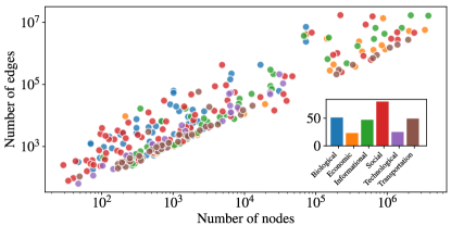
Figure 2: (Top) Number of nodes and edges for the networks in the corpus used in this work, and their domain composition (inset). (Bottom) Distribution of descriptor values for the networks in the corpus. The horizontal line marks the median values.

(a) Configuration model	(b) DCSBM

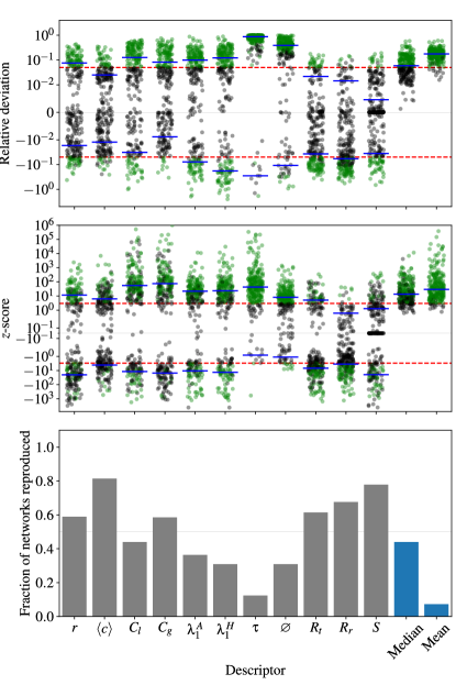
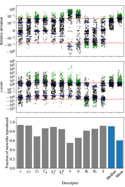
Figure 3: Distribution of relative deviation (top), $z$-score (middle), and fraction of networks reproduced (bottom) for (a) the configuration model and (b) the DCSBM, according to their respective predictive posterior distributions for each descriptor. We also show the median and mean of the absolute values for all descriptors for each network. The solid blue lines mark the negative and positive median values, and the dashed red line marks the values of $|\Delta|=0.05$ and $|z|=3$. The fraction of networks reproduced correspond to those that have the absolute value of either $\Delta$ or $z$ below these thresholds. The points in green color correspond to the networks that are not reproduced according to this combined criterion.

Figure 4: Relative deviation and $z$-score values for the global and mean local clustering coefficients, $C_{g}$ and $C_{l}$, as well as diameter and characteristic time of a random walk, $\varnothing$ and $\tau$, as a function of their empirical values, for every network in the corpus, when using the DCSBM. The dashed red line marks the values of $|\Delta|=0.05$ and $|z|=3$. The size of the symbol corresponds to the logarithm of the number of edges in the network, and the darkness to the mean degree.

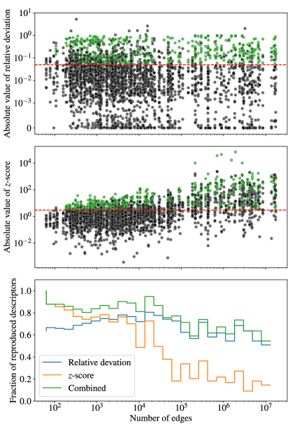
Figure 5: Absolute value of the relative deviation (top), $z$-score (middle) and fraction of reproduced descriptors (bottom), as a function of the number of edges, for every network in the corpus. The dashed red line marks the values of $|\Delta|=0.05$ and $|z|=3$. The fraction of descriptors reproduced correspond to those that have the value of either $\Delta$ or $z$ below these thresholds. The points in green color correspond to the descriptors that are not reproduced according to this combined criterion.

(a) Median
$z$-score	Relative deviation	Combined
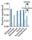
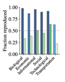
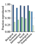
(b) Mean
$z$-score	Relative deviation	Combined

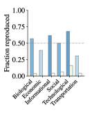
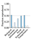
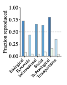
Figure 6: Fraction of reproduced networks according to their domain, considering the (a) median and (b) mean values of either the $z$-score, the relative deviations, or their combined values, for both models (as shown in the legend). When the combined values are used, this means that a model is deemed compatible with a network when we obtain either $|\Delta|<0.05$ or $|z|<3$.

Overall, since we know that a model like the DCSBM cannot possibly correspond to the true generative model of empirical networks, we should expect that in situations where the network is sufficiently large, and hence there is more abundant data, the values of the $z$-score will tend to be high. Here we argue that since the objective of a model like the DCSBM is to obtain a good approximation of the underlying model, not an exact representation, the ultimate criterion is a combination of the two, where we may deem the model compatible with the data when either the $z$-score or the relative deviation has a sufficiently low magnitude. For the purpose of clarity and simplicity of our analysis, we will consider the thresholds $|z|=3$ and $|\Delta|=0.05$ as reasonable choices to deem the model compatible with data, although our results will not depend on these particular choices, and we will always report the full range of values.

Before continuing, some important considerations regarding model checking should be made. While an excellent model should fulfill both of the above criteria simultaneously, we need to observe that a model that maximally overfits, i.e. ascribes to the observed network a probability of one, and to any other a probability of zero, will achieve the best possible performance according to both relative deviation and statistical significance. This occurs because we are using the same data to perform both the model inference and evaluate its quality, which is an invalid approach for model selection. Therefore, it is important to recognize the crucial difference between model checking and model selection: the latter attempts to find the model alternative that is better justified according to statistical evidence, while the former simply finds systematic discrepancies between the inferred model and data. In our analysis, protection against overfitting is obtained via Bayesian inference, and we use model checking only to evaluate the discrepancies (indeed, the fact we find discrepancies to begin with shows that we cannot be massively overfitting). Another observation is that when performing multiple comparison over many networks and descriptors, some amount of “statistically significant” deviations are always expected, even if the models inferred correspond to the true ones, unless we incorporate the fact that we are doing multiple comparisons in our criterion of statistical significance, which would be the methodologically correct approach. We will not perform such a correction in our analysis, because we do not seek to demonstrate the absolute quality of DCSBM as a ultimately plausible hypothesis for network formation. As we will see from our results, such a correction would gain us very little.

Finally, in Table 1 we list the network descriptors that are used in this work. Our approach requires scalar values, so we constrained ourselves to this category, and furthermore we chose quantities that can be computed quickly, so that robust statistics from the predictive posterior distributions can be obtained. Given these restrictions, we then chose descriptors that measure different aspects of the network structure, both at a local and global levels. Further details on the network descriptors are given in Appendix B.

IV Network corpus

We base our analysis on a corpus containing 275 networks spanning various domains and several orders of size magnitude, as shown in Fig. 2. We have not collected every network at our disposal, but instead chosen networks that are as diverse as possible, both in size and domain, and avoided many networks that are closely related by belonging to the same subset. In Appendix C we give more details about the datasets used.

V Results

In Fig. 3 we show the summaries of the posterior predictive checks for each descriptor and network, for both models considered. We observe a wide variety of deviation magnitudes, both for the same descriptors across networks, and across descriptors. As expected, the DCSBM results show systematically better agreement with the data when compared with the configuration model. Overall, the descriptors that show the worst agreement are the characteristic time of a random walk ($\tau$) and the diameter ($\varnothing$), both of which are particularly high for networks that are embedded in two dimensions, and for which the DCSBM is an inaccurate approximation (more on this below). Nevertheless, there is no single descriptor that the DCSBM does not capture for fewer than 50% of the networks. For descriptors like $S$, $R_{r}$, $R_{t}$ and ${\left<c\right>}$, the difference between the DCSBM and the configuration model are relatively minor, indicating that those can be captured to a substantial degree by the degree sequence alone.

When considering all descriptors simultaneously for each network, either by the median or mean of the absolute values of the $z$-score and relative deviation, we observe that a substantial majority of the networks considered show good agreement with the DCSBM, as opposed to the small minority that agree with the configuration model. The difference between the median and the mean indicates that there a sizeable fraction of the networks where the agreement is spoiled by a few outlier descriptors — typically $\tau$ and $\varnothing$.

The results obtained by the clustering coefficients are particularly interesting, since it is often the case that they are well reproduced by the DCSBM. This contrasts with what is commonly assumed, namely that the DCSBM should not be able to capture the abundance of triangles often seen in empirical networks, because in the limit where the number of groups is much smaller than the total number of nodes, the DCSBM becomes locally tree-like Decelle et al. (2011), with a vanishing probability of forming triangles. Therefore, we may imagine that the situations where there is an agreement with the DCSBM are those where the clustering values are low. However, as we see in Fig. 4(a) to (d), this is not quite true, and we observe good agreements even when the clustering values are high. This illustrates a point made in Ref. Peixoto (2021), that it is possible to obtain an abundance of triangles with the SBM simply by increasing the number of groups, in which case it can be explained as a byproduct of homophily. Indeed this is a situation we see in Fig. 4(a) to (d), where both the relative deviation and $z$-score values can be quite small even for extremal values of clustering. However, we do notice a substantial variability between agreements, and a fair amount of instances where the DCSBM cannot capture the observed clustering values, even when they are moderate or even small. This seems to indicate that there are a variety of processes capable of resulting in high clustering values, with homophily being only one of them Peixoto (2021). Overall, the mean local clustering values tend to be harder to reproduce than the global clustering values. In both cases, the $z$-scores are systematically high, indicating that the clustering values are in general a good criterion to reject the DCSBM as a statistically plausible model, although the relative deviation values tend to be lower than what one would naively expect, meaning that the model can still serve as a reasonably accurate approximation for clustered networks in many cases.

The behavior seen for the clustering coefficient is different for the diameter and characteristic time of a random walk, which are the least well reproduced descriptors, as shown Fig. 4(e) to (h). For both these descriptors — which are closely related, since a network with a large diameter will also tend to result in a slow mixing random walk — it is rare to find a network with very high empirical values which the DCSBM is able to accurately describe. Therefore it seems indeed that the DCSBM offers an inadequate ansatz to describe the structure of these networks, even by optimally adjusting its complexity.

In Fig. 5 we show how the model assessment depends on the size of the network. As one could expect, the $z$-score values tend to increase for larger networks, as more evidence becomes available against the plausibility of the DCSBM as the true generative model. However, the values of the relative deviation do not change appreciably for larger networks, indicating that it remains a good approximation regardless of the size of the system.

In Fig. 6 we show a summary of the fraction of all networks for which we obtain good agreement with either model, according to the network domains. Overall, we see that most domains show similar levels of agreements, except transportation and economic networks. Transportation networks are often embedded in two-dimensional spaces, resulting in large diameters and slow-mixing random walks. The economic networks considered also tend to show large values of these quantities, so the explanation for their discrepancy is the same.

V.1 Predicting quality of fit

Figure 7: Predictiveness of the quality of fit of the generative models considered, according to the empirical descriptor values, framed as a binary classification problem, as described in the text. (a) ROC curve for a leave-one-out random-forest classifier, (b) Gini feature importance for the configuration model, (c) same as (b) but for the DCSBM. Panels (d) and (e) show the best ROC AUC obtained for a set of descriptors of a given size, for the configuration model and DSCBM, respectively. Panels (f) and (g) show the same as (d) and (e), respectively, but with the number of edges excluded from the analysis.

Now we address the question of whether it is possible to predict the quality of fit of both models considered based solely on the empirical values of the networks descriptors. If we can isolate the descriptors which are most predictive, this would give us a general direction in which more accurate models could be constructed.

In order to evaluate the predictability, we frame it as a binary classification problem, where to each network $i$ is ascribed a binary value $y_{i}=0$ if we have simultaneously $|z_{i}|>3$ and $|\Delta_{i}|>0.05$, or otherwise $y_{i}=1$. The feature vector for each network is composed of the empirical values of the descriptors, $\bm{x}_{i}=(r,{\left<c\right>},C_{l},C_{g},\lambda_{1}^{A},\lambda_{1}^{H},\tau,\varnothing,R_{r},R_{t},S,E)$, with the addition of the number of edges $E$. For each network $i$, we train a random forest classifier on the entire corpus with that network removed, and evaluate the prediction score on the held-out network. We then repeat this procedure for all networks in the corpus, and evaluate how well the classifier is able to predict the binary label. We present the results of this experiment in Fig. 7 (top) which shows the receiver operating characteristic (ROC) curve, where the true positive rate and the false positive rate are plotted for all threshold values used to reach a classification. The area under the ROC curve (AUC), shown in the legend, can be equivalently interpreted as the probability that a randomly chosen true positive has a prediction score higher than a randomly chosen true negative. For the DCSBM and configuration model, we obtain an AUC value of 0.91 and 0.88, respectively. This indicates a fairly high predictability, from which we can conclude that it is indeed often possible to tell whether the models will provide a good or bad agreement, based only on the descriptor values.

Further insight can be obtained by inspecting the importance of each descriptor in the overall classification. We compute this via the so-called Gini importance, defined as the total decrease in node “impurity” (i.e. how often a node in decision tree contributes to a decision), weighted by the proportion of samples that reach that node, averaged over all trees in the classifier. The results can be seen in Fig. 7 (b) and (c). In both cases, we see that the number of edges is the most predictive descriptor, which is compatible with what we had already seen in Fig. 5, namely that the larger the networks are, the easier it becomes to reject a model according to the $z$-score. Otherwise, as one would expect, the importance of the remaining descriptors is largely compatible with their reproducibility shown in Fig. 3, where the descriptors that agree the least with the inferred models tend to be the most useful at predicting quality of fit beforehand.

This analysis allows us to emphasize two points: the characteristic time of a random walk $\tau$ and the diameter $\varnothing$, both extremal quantities of the network structure that are closely related, are the most difficult descriptors to be captured by the DCSBM. Therefore, an extension of the model that would cater for these properties would bring the most benefit across all networks. However, beyond these two descriptors, there is no substantial difference between the ones that remain, indicating that there is no obvious direction that would bring a systematic modelling improvement over all networks. On the other hand, as we show in Appendix B, the descriptor values and their predictive posterior deviations show nontrivial correlations, which means that if some of them are specifically targeted, it could potentially improve the quality of fit of other descriptors.

In order to understand what is the minimal amount of information required to predict the suitability of both models, and in this way remove the redundancy provided by the different descriptors, we computed the best ROC AUC obtained by a combination of descriptors of a given size, as shown in Fig. 7(d) and (e). In both cases we see that the predictability is saturated by only few descriptors. In the case of the configuration model most of the predictability is already achieved by a combination of $(C_{l},\tau,E)$. For the DCSBM we get instead $(r,\varnothing,E)$. If we remove the number of edges from the set of features (since it is not informative on the actual network structure), we obtain instead $(C_{g},\lambda_{1}^{A},\tau)$ and $(C_{l},\lambda^{H}_{1},\varnothing)$, for the configuration model and DCSBM, respectively. It should be emphasized that if a descriptor does not appear in the minimal set this does not mean it is not predictive of the quality of fit, only that it offers largely redundant information in that regard. Thus, for both models if we replace $\varnothing$ with $\tau$ or $\lambda^{H}_{1}$ with $\lambda_{1}^{A}$, etc, we get similar results. This suggests that, besides spatial embeddedness (which influence $\varnothing$ and $\tau$ the most), the addition of explicit mechanisms for triangle formation (which affects $C_{g},C_{l},\lambda^{H}_{1},\lambda^{A}_{1}$ directly) might improve the overall expressiveness of the DCSBM — which in fact has been observed in a more limited dataset Peixoto (2021).

VI Conclusion

We performed a systematic analysis of posterior predictive checks of the SBM on a diverse corpus of empirical networks, spanning a broad range of sizes and domains. Using a variety of network descriptors, we observed that the SBM is able to accurately capture the structure of the majority of networks in the corpus. The types of networks that show the worst agreement with DCSBM tend to possess a large diameter and a slow mixing of random walks — features that are commonly associated with a low-dimensional spatial embedding, and a violation of the “small-world” property. For the other kinds of networks the agreement tends to be fairly good, even for many networks with an abundance of triangles, in contradiction to what is commonly assumed to be possible with this class of models.

We have also identified the minimal set of network descriptors capable of predicting the quality of fit of the SBM, which is composed of the network diameter and characteristic time of a random walk as the most important, followed by clustering as a secondary feature. This points to the most productive directions in which this class of models could be improved.

One of the limitations of our analysis is that it is conditioned on the set of descriptors used, and thus shortcomings or successes of the model with respect to other properties not analysed are not uncovered. A natural extension of our work would be to consider an even broader set of descriptors that could reveal more relevant dimensions for the comparison. This kind of analysis is open ended, as there is no short supply of possible network descriptors. We hope our work will motivate further study in this direction, and with a larger variety of generative models within or beyond the SBM family.

Aknowledgements

The computational results presented have been achieved using the Vienna Scientific Cluster (VSC).

Appendix A Posterior predictive sampling

As described in the main text, we obtain samples from the posterior predictive distribution of Eq. 5 by first sampling from the posterior distribution of Eq. 4 using MCMC and then generating new networks from the inferred models. More specifically, we sample $(\bm{A},\bm{k},\bm{e},\bm{b})$ from

$$P(\bm{A},\bm{k},\bm{e},\bm{b}|\bm{G})=\frac{P(\bm{G}|\bm{A})P(\bm{A}|\bm{k},\bm{e},\bm{b})P(\bm{k},\bm{e},\bm{b})}{P(\bm{G})},$$ (8)

using the merge-split MCMC of Ref. Peixoto (2020b), together with the agglomerative initialization heuristic of Refs. Peixoto (2014b, a), and the multigraph edge moves of Ref. Peixoto (2020a). For networks of size up to $E=10^{5}$ edges we observe good equilibration of the MCMC runs, but for large networks it becomes too slow. For these large networks we settle for a point estimate of the partition $\bm{b}$ obtained by several runs of the initialization algorithm and keeping the best result, and then we equilibrate the chain according to $\bm{A}$ alone (which affects $\bm{k}$ and $\bm{e}$), which tends to happen quickly. We have verified that performing this calculation several times yields very similar results. The only noticeable outcome of this shortcut for larger networks is that it tends to reduce the variance of the posterior predictive distributions, which can potentially contribute to the elevated $z$-scores we obtained in our analysis. However, since the relative deviation values we obtained did not seem to depend on the size of the network, this gives us confidence that this approach does not introduce significant biases.

Given a sample $(\bm{A},\bm{k},\bm{e},\bm{b})$, we are interested only in $(\bm{k},\bm{e},\bm{b})$ (and hence samples from their marginal distribution), so we discard $\bm{A}$ and sample a new multigraph $\bm{A}^{\prime}$ from the model of Eq. 1. This can be done exactly with an efficient algorithm that works similarly to what was proposed in Refs. Parkkinen et al. (2009); Rohe et al. (2018), but is valid for the microcanonical model: Given the parameters $(\bm{k},\bm{e},\bm{b})$ we proceed by creating for each group $r$ a multiset of candidate nodes $\bm{v}_{r}$, containing $k_{i}$ copies of each node $i$ with $b_{i}=r$. Then, for each group pair $(r,s)$ with $r\leq s$ and $e_{rs}>0$, we repeat the following three steps for an $e_{rs}$ number of times (or $e_{rs}/2$ if $r=s$):

1. We sample a node $i$ from the multiset $\bm{v}_{r}$ uniformly at random, and we remove it from the multiset.

2. We sample a node $j$ from the multiset $\bm{v}_{s}$ uniformly at random, and we remove it from the multiset.

3. We add an edge $(i,j)$ to $\bm{A}$ (i.e. increment $A_{ij}$ by one, or two if $i=j$).

The resulting multigraph $\bm{A}$ is sampled exactly with a probability given by Eq.1. Since the number of nonzero entries of $\bm{e}$ cannot be larger than the total number of edges $E$, the whole algorithm finishes in time $O(N+E)$, where $N$ is the number of nodes.

Given a sample $\bm{A}$, we obtain a simple graph $\bm{G}$ simply by removing all self-loops and truncating the edge multiplicities, i.e.

$$G_{ij}=\begin{cases}1,\text{ if }A_{ij}>0\text{ and }i\neq j,\\ 0,\text{ otherwise}.\end{cases}$$ (9)

Finally, given $\bm{G}$ we compute the network descriptor $f(\bm{G})$ of interest.

A C++ implementation of every algorithm used in this analysis is freely available as part of the graph-tool library Peixoto (2014c).

Appendix B Network descriptors

Figure 8: Absolute value of the $z$-score versus absolute value of relative deviation, for every descriptor value and network in the corpus, according to (a) the configuration model and (b) the DCSBM. The dashed lines mark the values $|z|=3$ and $|\Delta|=0.05$, and the histograms the marginal distributions. The solid blue lines mark the median values.

Figure 9: (a) Kendall’s correlation coefficient $\tau$ between pairs of descriptor values across all networks in the corpus. Panels (b) and (c) show the same but for $z$-score and relative deviation values, respectively, according to the DCSBM. The insets show the correlation between coefficients from each respective panel and panel (a).

Below are the definitions of the descriptors used in our analyses.

Degree assortativity, $r$

Defined as Newman (2003)

$$r=\frac{\sum_{kk^{\prime}}kk^{\prime}(m_{kk^{\prime}}-m_{k}m_{k^{\prime}})}{\sigma_{k}\sigma_{k^{\prime}}},$$

where $m_{kk^{\prime}}$ is the fraction of edges with endpoints of degree $k$ and $k^{\prime}$, $m_{k}=\sum_{k^{\prime}}m_{kk^{\prime}}$, and $\sigma_{k}$ is the standard deviation of $m_{k}$.

Mean $k$-core, ${\left<c\right>}$

The $k$-core is a maximal set of vertices such that its induced subgraph only contains vertices with degree larger than or equal to $k$. The $k$-core value $c_{i}$ of node $i$ is the largest value of $k$ for which $i$ belongs to the $k$-core. The mean value is then

$${\left<c\right>}=\frac{1}{N}\sum_{i}c_{i}.$$

This can be computed in time $O(N+E)$ according to the algorithm of Ref. Batagelj and Zaveršnik (2011).

Mean local clustering coefficient, $C_{l}$

The local clustering coefficient Watts and Strogatz (1998a) of node $i$ is given by

$$C_{i}=\frac{\sum_{jk}G_{ij}G_{ki}G_{jk}}{k_{i}(k_{i}-1)}.$$

It measures the fraction of pairs of neighbors that are also connected. The mean value is then just

$$C_{l}=\frac{1}{N}\sum_{i}C_{i}.$$

Global clustering coefficient, $C_{g}$

The global clustering coefficient of is given by

$$C_{g}=\frac{\sum_{ijk}G_{ij}G_{ki}G_{jk}}{\sum_{i}k_{i}(k_{i}-1)}.$$

It measures the fraction of connected triads that close to form a triangle.

Leading eigenvalue of adjacency matrix, $\lambda_{1}^{A}$

The leading eigenvalue of the adjacency matrix is the largest value of $\lambda$ which solves

$$\bm{G}\bm{x}=\lambda\bm{x},$$

where $\bm{x}$ is the associated eigenvector.

Leading eigenvalue of Hashimoto matrix, $\lambda_{1}^{H}$

The leading eigenvalue of the Hashimoto (a.k.a. non-backtracking) matrix Hashimoto (1989) is the largest value of $\lambda$ which solves

$$\bm{H}\bm{x}=\lambda\bm{x},$$

where $\bm{x}$ is the associated eigenvector, and $\bm{H}$ is an asymmetric $E\times E$ matrix with entries defined as

$$H_{k\to l,i\to j}=\begin{cases}1&\text{if }G_{kl}=G_{ij}=1,l=i,k\neq j,\\ 0&\text{otherwise}.\end{cases}$$

Characteristic time of a random walk, $\tau$

The characteristic time of a random walk is obtained via the second largest eigenvalue $\lambda_{2}^{T}\in[0,1]$ of the transition matrix $\bm{T}$, with entries

$$T_{ij}=\frac{G_{ij}}{k_{j}},$$

where $k_{i}=\sum_{j}G_{ji}$. It is defined as

$$\tau=-\ln\lambda_{2}^{T}.$$

If the network is disconnected, we compute $\tau$ only on the largest component.

Pseudo-diameter, $\varnothing$

The pseudo-diameter is an approximate graph diameter. It is obtained by starting from an arbitrary source node, and finding a target node that is farthest away from the source. This process is repeated by treating the target as the new starting node, and ends when the graph distance no longer increases. This graph distance is taken to be the pseudo-diameter. The algorithm runs in time $O(N+E)$.

If the network is disconnected, $\varnothing$ is taken as the maximum of pseudo-diameters of the connected components.

Node percolation profile (random removal), $R_{r}$

We chose a random node order, and remove nodes sequentially from the graph according to it. If $S_{i}$ is the fraction of nodes in the largest component after the $i$-th removal, then the profile value is

$$R_{r}=\frac{1}{N}\sum_{i}S_{i}.$$

The value is averaged over several node orderings.

Node percolation profile (targeted removal), $R_{t}$

The computation is the same as $R_{r}$, but the nodes are always removed in decreasing order of the degree.

Fraction of nodes in the largest component, $S$

A component is a maximal set of nodes that are connected by a path. The largest component is the component with the largest number of nodes, and $S$ is the fraction of all nodes that belong to it.

In Fig. 8 we show how the $z$-scores and relative deviation values are related for every network descriptor, according to both models used. In Fig. 9 we show Kendall’s $\tau$ correlation coefficient among the descriptor values themselves, as well as their $z$-scores and relative deviations, according to the DCSBM. The insets show how the correlations among the deviations are themselves also correlated with the descriptor correlations.

Appendix C Dataset descriptions

Below are descriptions of the network datasets used in this work. The codenames in the first row correspond to the respective entries in the Netzschleuder repository Peixoto (2020c) where the networks can be downloaded. Some of the descriptions were obtained from the Colorado Index of Complex Networks Clauset et al. (2016).

For all networks, the versions considered in this work were transformed into simple graphs, i.e. symmetrized versions of directed networks and/or with parallel edges and self-loops removed.

Name	Description	$N$	$E$	Domain
blumenau_drug	A network of drug-drug interactions, extracted from 18 months of electronic health records (EHRs) from the city of Blumenau in Southern Brazil Brattig Correia et al. (2019).	75	181	Biological
budapest_connectome (1)	Brain graphs derived from connectomes of 477 people, computed from the Human Connectome Project Szalkai et al. (2015).	$1015$	$53586$	Biological
budapest_connectome (2)		1015	62552	Biological
celegans_2019 (1)	Networks among neurons of both the adult male and adult hermaphrodite worms C. elegans, constructed from electron microscopy series, to include directed edges (chemical) and undirected (gap junction), and spanning including nodes for muscle and non-muscle end organs Cook et al. (2019).	$514$	$2832$	Biological
celegans_2019 (2)		575	4500	Biological
celegans_2019 (3)		454	4172	Biological
celegans_2019 (4)		469	1433	Biological
celegans_interactomes (1)	Ten networks of protein-protein interactions in Caenorhabditis elegans (nematode), from yeast two-hybrid experiments, biological process maps, literature curation, orthologous interactions, and genetic interactions Simonis et al. (2008).	$2724$	$13564$	Biological
celegans_interactomes (2)		912	22738	Biological
celegans_interactomes (3)		537	517	Biological
collins_yeast	Network of protein-protein interactions in Saccharomyces cerevisiae (budding yeast), measured by co-complex associations identified by high-throughput affinity purification and mass spectrometry (AP/MS) Collins et al. (2007).	1622	9070	Biological
ecoli_transcription (1)	Network of operons and their pairwise interactions for E. coli Shen-Orr et al. (2002).	$423$	$519$	Biological
foodweb_baywet	Networks of carbon exchanges among species in the cypress wetlands of South Florida. One network covers the wet and the other the dry season Ulanowicz and DeAngelis (1999).	128	2075	Biological
foodweb_little_rock	A food web among the species found in Little Rock Lake in Wisconsin Martinez (1991).	183	2434	Biological
fresh_webs (1)	Trophic-level species interactions in streams in New Zealand, Maine and North Carolina Thompson and Townsend (2003).	$94$	$424$	Biological
fresh_webs (2)		107	965	Biological
genetic_multiplex (1)	Multiplex networks representing different types of genetic interactions, for different organisms. Layers represent (i) physical, (ii) association, (iii) co-localization, (iv) direct, and (v) suppressive, (vi) additive or synthetic genetic interaction De Domenico et al. (2014).	$2640$	$3677$	Biological
genetic_multiplex (2)		1005	1155	Biological
genetic_multiplex (3)		313	325	Biological
genetic_multiplex (4)		6570	223542	Biological
human_brains (1)	Networks of neural interactions extracted from human patients using the Magnetic Resonance One-Click Pipeline (MROCP), where nodes are voxels of neural tissue and edges represent connections by single fibers Gray Roncal et al. (2013).	$1215$	$13768$	Biological
human_brains (2)		200	1231	Biological
human_brains (3)		139	873	Biological
human_brains (4)		1771	3645	Biological
human_brains (5)		1105	19543	Biological
human_brains (6)		1527	3939	Biological
human_brains (7)		70	1219	Biological
human_brains (8)		200	2808	Biological
human_brains (9)		70	1301	Biological
human_brains (10)		1632	5218	Biological
human_brains (11)		16783	430493	Biological
human_brains (12)		72783	2411659	Biological
human_brains (13)		72783	3720694	Biological
human_brains (14)		72783	4205222	Biological
human_brains (15)		72783	7175769	Biological
interactome_figeys	A network of human proteins and their binding interactions Ewing et al. (2007).	2239	6432	Biological
interactome_yeast	A network of protein-protein binding interactions among yeast proteins Coulomb et al. (2005).	1870	2203	Biological
kegg_metabolic (1)	Metabolic networks of various species, as extracted from the Kyoto Encyclopedia of Genes and Genomes (KEGG) database in March 2006 Huss and Holme (2007).	$1031$	$2485$	Biological
kegg_metabolic (2)		1917	5803	Biological
kegg_metabolic (3)		505	1144	Biological
macaque_neural	A network of cortical regions in the Macaque cortex 199 (1993).	47	313	Biological
malaria_genes (1)	Networks of recombinant antigen genes from the human malaria parasite P. falciparum Larremore et al. (2013).	$307$	$2684$	Biological
malaria_genes (2)		307	3961	Biological
malaria_genes (3)		307	7579	Biological
malaria_genes (4)		307	2812	Biological
messal_shale	A network of feeding links among taxa based on the 48 million years old uppermost early Eocene Messel Shale Dunne et al. (2014).	700	6395	Biological
nematode_mammal	A global interaction web of interactions between nematodes and their host mammal species, extracted from the helminthR package and dataset Dallas et al. (2018).	30516	61597	Biological
plant_pol_kato	A bipartite network of plants and pollinators from Kyoto University Forest of Ashu, Japan, from 1984 to 1987 Kato et al. (1988).	772	1206	Biological
plant_pol_robertson	A bipartite network of plants and pollinators, from southwestern Illinois, USA Robertson (1928).	1884	15255	Biological
reactome	A network of human proteins and their binding interactions, extracted from Reactome project Joshi-Tope (2004).	6327	146160	Biological
yeast_transcription	Network of operons and their pairwise interactions, via transcription factor-based regulation, within the yeast Saccharomyces cerevisiae Milo et al. (2002).	916	1081	Biological
caida_as	Autonomous System (AS) relationships on the Internet, from 2004-2007 cai (2009).	$8020$	$18203$	Technological
gnutella (1)	Gnutella peer-to-peer file sharing network from 5-31 August 2002 Ripeanu and Foster (2002).	$6301$	$20777$	Technological
gnutella (2)		22687	54705	Technological
internet_as	A symmetrized snapshot of the structure of the Internet at the level of Autonomous Systems (ASs), reconstructed from BGP tables posted by the University of Oregon Route Views Project Karrer et al. (2014).	22963	48436	Technological
internet_top_pop (1)	Assorted snapshots of internet graph at the Point of Presence (PoP) level (which lies between the IP and AS levels), collected from around the world and at various times. The earliest snapshots are for ARPANET (1969-1972), with a few more from pre-2000 Knight et al. (2011).	$76$	$115$	Technological
internet_top_pop (2)		145	186	Technological
internet_top_pop (3)		47	63	Technological
internet_top_pop (4)		197	243	Technological
internet_top_pop (5)		754	895	Technological
jdk	A network of class dependencies within the JDK (Java SE Development Kit) 1.6 Kunegis (2013).	6434	53658	Technological
jung	A network of software class dependency within the JUNG 2.0 Šubelj and Bajec (2012a).	6120	50290	Technological
linux	A network of Linux (v3.16) source code file inclusion Kunegis (2013).	30837	213217	Technological
power	A network representing the Western States Power Grid of the United States Watts and Strogatz (1998b).	4941	6594	Technological
route_views (1)	733 daily network snapshots denoting BGP traffic among autonomous systems (ASs) on the Internet, from the Oregon Route Views Project, spanning 8 November 1997 to 2 January 2000. Data collected by NLANR/MOAT rou (2001).	$103$	$239$	Technological
route_views (2)		512	1181	Technological
route_views (3)		767	1734	Technological
route_views (4)		1486	3172	Technological
route_views (5)		6474	12572	Technological
route_views (6)		6301	12226	Technological
software_dependencies (1)	Several networks of software dependencies. Nodes represent libraries and a directed edge denotes a library dependency on another Šubelj and Bajec (2012a, b).	$388$	$514$	Technological
software_dependencies (2)		838	1063	Technological
software_dependencies (3)		799	3579	Technological
software_dependencies (4)		550	1153	Technological
software_dependencies (5)		282	505	Technological
software_dependencies (6)		2124	4809	Technological
topology	An integrated snapshot of the structure of the Internet at the level of Autonomous Systems (ASs), reconstructed from multiple sources, including the RouteViews and RIPE BGP trace collectors, route servers, looking glasses, and the Internet Routing Registry databases Zhang et al. (2005).	34761	107720	Technological
adjnoun	A network of word adjacencies of common adjectives and nouns in the novel “David Copperfield” by Charles Dickens Newman (2006).	112	425	Informational
bag_of_words	Five text collections in the form of bags-of-words Newman (2019); Dua and Graff (2019).	$67963$	$3710420$	Informational
baidu	Four networks from Chinese online encyclopedias Baidu Niu et al. (2011).	2141300	17014946	Informational
berkstan_web	The web graph of Berkeley and Stanford Universities Leskovec et al. (2009).	685231	6649470	Informational
bible_nouns	A network of noun phrases (places and names) in the King James Version of the Bible C. Römhild .	1773	9131	Informational
citeseer	Citations among papers indexed by the CiteSeer digital library Bollacker et al. (1998).	384413	1736145	Informational
cora	Citations among papers indexed by CORA, from 1998, an early computer science research paper search engine McCallum et al. (2000).	23166	89157	Informational
dblp_cite	Citations among papers contained in the DBLP computer science bibliography Ley (2002).	12590	49636	Informational
dbtropes_feature	A bipartite network of artistic works (movies, novels, etc.) and their tropes (stylistic conventions or devices), as extracted from tvtropes Kunegis (2013).	152093	3232134	Informational
discogs_label	Two bipartite networks of the affiliations between musical labels and either musical genres or musical “styles,” as given in the discogs.com database Kunegis (2013).	270786	481661	Informational
edit_wikibooks (1)	Two bipartite user-page networks extracted from Wikipedia, about books Foundation (2019).	$1162$	$1213$	Informational
edit_wikibooks (2)		1584	1748	Informational
edit_wikibooks (3)		7177	7732	Informational
edit_wikinews (1)	Two bipartite user-page networks extracted from Wikipedia, about news events Foundation (2019).	$2511$	$4986$	Informational
edit_wikinews (2)		4523	8891	Informational
edit_wikinews (3)		5541	10545	Informational
edit_wikinews (4)		2208	2753	Informational
edit_wikinews (5)		4457	5942	Informational
edit_wikiquote (1)	A bipartite user-page network extracted from Wikiquotes Foundation (2019).	$270$	$243$	Informational
edit_wikiquote (2)		1041	1109	Informational
edit_wikiquote (3)		704	800	Informational
edit_wikiquote (4)		1333	2731	Informational
edit_wikiquote (5)		625	823	Informational
edit_wiktionary (1)	Three bipartite user-page networks extracted from Wiktionary, for French, German, and English Foundation (2019).	$271$	$285$	Informational
edit_wiktionary (2)		289	276	Informational
edit_wiktionary (3)		1271	1270	Informational
edit_wiktionary (4)		8552	34589	Informational
edit_wiktionary (5)		3016	6263	Informational
google_web	A web graph representing a crawl of a portion of the general WWW, from a 2002 Google Programming contest Leskovec et al. (2009).	916428	4322051	Informational
movielens_100k	Three bipartite networks that make up the MovieLens 100K Dataset, a stable benchmark dataset of 100,000 ratings from 1000 users on 1700 movies Research (2019).	24129	71154	Informational
polblogs	A directed network of hyperlinks among a large set of U.S Adamic and Glance (2005).	1490	16715	Informational
polbooks	A network of books about U.S Pasternak and Ivask (1970).	105	441	Informational
scotus_majority (1)	Network of legal citations by the US Supreme Court (SCOTUS) Fowler and Jeon (2008); Fowler et al. (2007).	$25417$	$216456$	Informational
trec_web	A web graph network originally constructed in 2003 as a testbed for information-retrieval techniques, including web search engines Bailey et al. (2003).	1601787	6679248	Informational
unicodelang	A bipartite network of languages and the countries in which they are spoken, as estimated by Unicode Kunegis (2013).	868	1255	Informational
us_patents	Citations among patents in the United States, as found in the National Bureau of Economic Research (NBER) database, from 1975 to 1999 Hall et al. (2001).	3774768	16518947	Informational
webkb (1)	Web graphs crawled from four Computer Science departments in 1998, with each page manually classified into one of 7 categories: course, department, faculty, project, staff, student, or other Slattery and Craven (1998).	$286$	$493$	Informational
webkb (2)		433	954	Informational
webkb (3)		300	565	Informational
webkb (4)		349	696	Informational
webkb (5)		348	16625	Informational
wiki_science	A network of scientific fields, extracted from the English Wikipedia in early 2020 Calderone (2020).	687	6523	Informational
word_adjacency (1)	Networks of word adjacency in texts of several languages including English, French, Spanish and Japanese Milo et al. (2004).	$8325$	$23841$	Informational
word_adjacency (2)		2704	7998	Informational
word_assoc	A network of word associations showing the count of such associations as collected from subjects, from the Edinburgh Associative Thesaurus (EAT) Kiss et al. (1973).	23132	297094	Informational
wordnet	A network of English words from the WordNet, denoting relationships between words (synonymy, hyperonymy, meronymy, etc.) Fellbaum (2010)	146005	656999	Informational
yahoo_ads	A network of words extracted from phrases on which advertisers bid, in Yahoo! advertisements Kunegis (2013).	653260	2931698	Informational
chicago_road	A transportation network of Chicago, USA, from an unknown date (probably late 20th century) Stabler (2021).	12982	20627	Transportation
contiguous_usa	A network of contiguous states in the USA, in which each state is a node and two nodes are connected if they share a land-based geographic border Knuth (1993).	49	107	Transportation
eu_airlines	A multiplex network of airline routes among European airports, where each of the 37 edge types represents routes by a different airline Cardillo et al. (2013).	450	2953	Transportation
euroroad	A network of international “E-roads,” mostly in Europe Šubelj and Bajec (2011).	1174	1417	Transportation
faa_routes	A network of air traffic routes, from the FAA (Federal Aviation Administration) National Flight Data Center (NFDC) preferred routes database Administration (2010).	1226	2408	Transportation
london_transport	Multiplex network with 3 edge types representing links within the three layers of London train stations: Underground, Overground and DLR De Domenico et al. (2014).	369	430	Transportation
openflights	A network of regularly occurring flights among airports worldwide, extracted from the openflights.org dataset ope (2019).	3214	18858	Transportation
openstreetmap (1)	The road network for the entire United States, as extracted from the OpenStreetMap project Boeing (2019).	$351$	$434$	Transportation
openstreetmap (2)		354	350	Transportation
openstreetmap (3)		831	923	Transportation
openstreetmap (4)		1603	2188	Transportation
openstreetmap (5)		4240	5102	Transportation
openstreetmap (6)		8904	10549	Transportation
openstreetmap (7)		724	1048	Transportation
openstreetmap (8)		2371	3295	Transportation
openstreetmap (9)		684	823	Transportation
openstreetmap (10)		500	780	Transportation
openstreetmap (11)		3377	4698	Transportation
openstreetmap (12)		1609	1972	Transportation
openstreetmap (13)		612	688	Transportation
openstreetmap (14)		209734	297196	Transportation
roadnet (1)	Road networks from three US states (CA, PA, TX), in which edges are stretches of road and vertices are intersections of roads Leskovec et al. (2009).	$1971281$	$2766607$	Transportation
roadnet (2)		1090920	1541898	Transportation
roadnet (3)		1393383	1921660	Transportation
urban_streets (1)	Urban street networks, corresponding to 1-square-mile maps of 20 cities around the world Crucitti et al. (2006); Latora et al. (2017).	$179$	$230$	Transportation
urban_streets (2)		240	339	Transportation
urban_streets (3)		467	691	Transportation
urban_streets (4)		248	418	Transportation
urban_streets (5)		697	1084	Transportation
urban_streets (6)		169	271	Transportation
urban_streets (7)		1840	2397	Transportation
urban_streets (8)		1496	2252	Transportation
urban_streets (9)		584	958	Transportation
urban_streets (10)		217	222	Transportation
urban_streets (11)		541	771	Transportation
urban_streets (12)		252	328	Transportation
urban_streets (13)		869	1307	Transportation
urban_streets (14)		192	302	Transportation
urban_streets (15)		210	323	Transportation
urban_streets (16)		2870	4375	Transportation
urban_streets (17)		335	494	Transportation
urban_streets (18)		488	729	Transportation
urban_streets (19)		169	196	Transportation
us_air_traffic	Yearly snapshots of flights among all commercial airports in the United States from 1990 to today us_ (2017).	2278	58228	Transportation
us_roads (1)	The road networks of the 50 US States and the District of Columbia based on UA Census 2000 TIGER/Line Files us_ (2002).	$9559$	$14841$	Transportation
us_roads (2)		194505	212345	Transportation
us_roads (3)		330386	431398	Transportation
us_roads (4)		630639	705083	Transportation
us_roads (5)		716215	886897	Transportation
7th_graders	A network of friendships among 29 seventh grade students in Victoria, Australia Mathews (1976).	29	250	Social
academia_edu	Snapshot of the follower relationships among users of academia.edu, a platform for academics to share research papers, scraped in 2011 Fire et al. (2013).	200169	1022441	Social
add_health (1)	A directed network of friendships obtained through a social survey of high school students in 1994. The ADD HEALTH data are constructed from the in-school questionnaire; 90,118 students representing 84 communities took this survey in 1994-95 Moody (2001).	$900$	$1648$	Social
add_health (2)		1929	7035	Social
add_health (3)		1282	3487	Social
add_health (4)		111	378	Social
add_health (5)		74	358	Social
add_health (6)		624	1745	Social
add_health (7)		1755	4017	Social
arxiv_authors (1)	Scientific collaborations between authors of papers submitted to arxiv.org Leskovec et al. (2007a).	$26197$	$14484$	Social
arxiv_collab	Collaboration graphs for scientists, extracted from the arXiv (physics) Newman (2001).	$8361$	$15751$	Social
bitcoin_alpha	A network of who-trusts-whom relationships among users of the Bitcoin Alpha platform Kumar et al. (2016).	3783	14124	Social
ceo_club	A bipartite network of the memberships of chief executive officers and the social organizations (clubs) to which they belong, from the Minneapolis-St. Paul area Faust (1997).	40	95	Social
chess	A network among chess players (nodes) giving the chess match outcomes (edges), for game-by-game results among the world’s top chess players Kaggle .	7301	55899	Social
copenhagen (1)	A network of social interactions among university students within the Copenhagen Networks Study, over a period of four weeks, sampled every 5 minutes Sapiezynski et al. (2019).	$536$	$621$	Social
copenhagen (2)		800	6418	Social
copenhagen (3)		568	697	Social
crime	A network of associations among suspects, victims, and/or witnesses involved in crimes in St. Louis in the 1990s Decker et al. (1991).	1380	1476	Social
cs_department	Multiplex network consisting of 5 edge types corresponding to online and offline relationships (Facebook, leisure, work, co-authorship, lunch) between employees of the Computer Science department at Aarhus Magnani et al. (2013).	61	353	Social
dbpedia_country	A bipartite network of the affiliations between notable people and countries of the world, as extracted from Wikipedia via the DBpedia project Auer et al. (2007).	592414	624402	Social
dbpedia_occupation	A bipartite network of the affiliations between notable people and occupations, as extracted from Wikipedia by the DBpedia project Auer et al. (2007).	229307	250945	Social
dnc	A network representing the exchange of emails among members of the Democratic National Committee, in the email data leak released by WikiLeaks in 2016 Kunegis (2013).	2029	10429	Social
dolphins	An undirected social network of frequent associations observed among 62 dolphins (Tursiops) in a community living off Doubtful Sound, New Zealand, from 1994-2001 Lusseau et al. (2003).	62	159	Social
ego_social (1)	Ego networks associated with a set of accounts of three social media platforms (Facebook, Google+, and Twitter) Mcauley and Leskovec (2014).	$150$	$1693$	Social
ego_social (2)		747	30025	Social
ego_social (3)		452	12513	Social
email_company	A network of emails among employee email addresses at a mid-sized manufacturing company Michalski et al. (2011).	167	3250	Social
email_enron	The Enron email corpus, containing all the email communication from the Enron corporation, which was made public as a result of legal action Klimt and Yang (2004).	36692	183831	Social
escorts	A bipartite network of escort and individuals who buy sex from them in Brazil, extracted from a Brazilian online community for such ratings Rocha et al. (2011).	16730	39044	Social
facebook_friends	A small anonymized Facebook ego network, from April 2014. Nodes are Facebook profiles, and an edge exists if the two profiles are “friends” on Facebook Maier and Brockmann (2017).	362	1988	Social
facebook_organizations (1)	Six networks of friendships among users on Facebook who indicated employment at one of the target corporation Fire and Puzis (2015).	$320$	$2369$	Social
facebook_organizations (2)		165	726	Social
facebook_organizations (3)		1429	19357	Social
facebook_organizations (4)		3862	87324	Social
facebook_organizations (5)		5793	30753	Social
facebook_organizations (6)		5524	94218	Social
facebook_wall	Friendship relationships and interactions (wall posts) for a subset of the Facebook social network in 2009, recorded over a 2 year period Viswanath et al. (2009).	46952	183412	Social
fediverse	An early snapshot of the federation network among web publishers using the ActivityPub protocol Rochko (2018).	4860	426351	Social
flickr_groups	Bipartite networks of the affiliations between users and groups on several online social network sites, including Flickr, YouTube, LiveJournal, and Orkut, extracted in 2007 Mislove et al. (2007).	499610	8545307	Social
football_tsevans	A network of American football games between Division IA colleges during regular season Fall 2000 Girvan and Newman (2002); Evans (2010).	115	613	Social
foursquare (1)	Two bipartite networks of users and restaurant locations in New York City on Foursquare, from 24 October 2011 to 20 February 2012 Yang et al. (2013).	$6410$	$9472$	Social
foursquare (2)		4936	13472	Social
highschool	A network of friendships among male students in a small high school in Illinois from 1958 Harper and Coleman (1965).	70	274	Social
hiv_transmission	A set of networks of HIV transmissions between people through sexual, needle-sharing, or social connections, based on combining 8 datasets collected from 1988 to 2001 Morris and Rothenberg (2011).	35229	48889	Social
hyves	A network of friendships among users of Hyves, an online social networking site in the Netherlands (comparable to Facebook at the time) Zafarani and Liu (2009).	1402673	2777419	Social
jazz_collab	The network of collaborations among jazz musicians, and among jazz bands, extracted from The Red Hot Jazz Archive digital database, covering bands that performed between 1912 and 1940 Gleiser and Danon (2003).	198	2742	Social
karate (1)	Network of friendships among members of a university karate club Zachary (1977).	$34$	$78$	Social
kidnappings	Bipartite network of members of the Abu Sayyaf Group in the Philippines, and the kidnapping events they were involved in Gerdes et al. (2014).	351	402	Social
lastfm (1)	User-band networks from the music website last.fm Celma (2010).	$175069$	$898062$	Social
lesmis	The network of scene coappearances of characters in Victor Hugo’s novel "Les Miserables". Edge weights denote the number of such occurrences Knuth (1993).	77	254	Social
libimseti	A network of ratings given between users at Libimseti.cz, a Czech online dating website Kunegis et al. (2012).	220970	17233144	Social
mislove_osn (1)	Network structure for four large online social networks Mislove et al. (2007).	$1138499$	$2990443$	Social
netscience	A coauthorship network among scientists working on network science, from 2006. This network is a one-mode projection from the bipartite graph of authors and their scientific publications Newman (2006).	1589	2742	Social
new_zealand_collab	A network of scientific collaborations among institutions in New Zealand Aref et al. (2018).	1511	4273	Social
petster	A network of friendships among users on catster.com and dogster.com Kunegis (2013).	623766	15695166	Social
physician_trust	A network of trust relationships among physicians in four midwestern (USA) cities in 1966 Coleman et al. (1957).	241	923	Social
physics_collab	Coauthorships among the Pierre Auger Collaboration of physicists De Domenico et al. (2015a).	$514$	$6482$	Social
reality_mining	A network of human proximities among students at Massachusetts Institute of Technology (MIT), as measured by personal mobile phones Eagle and (Sandy).	96	2539	Social
residence_hall	A network of friendships among students living in a residence hall at Australian National University Freeman et al. (1998).	217	1839	Social
sp_high_school (1)	Contacts and friendship relations between students in a high school in Marseilles, France, in December 2013 Mastrandrea et al. (2015).	$329$	$348$	Social
sp_high_school (2)		329	406	Social
sp_high_school_new	Network of contacts between students in a high school in Marseilles, France De Domenico et al. (2014).	$126$	$1709$	Social
sp_hypertext	Network of contacts among attendees of the ACM Hypertext 2009 conference Isella et al. (2011).	$113$	$2196$	Social
sp_office	A temporal network of contacts between individuals, measured in an office building in France, from June 24 to July 3, 2013 Génois et al. (2015).	92	755	Social
sp_primary_school	Network of contacts among students and teachers at a primary school in Lyon, France, on consecutive days of in October 2009 Stehlé et al. (2011).	242	8317	Social
student_cooperation	Network of cooperation among students in the “Computer and Network Security” course at Ben-Gurion University, in 2012 Fire et al. (2012).	185	311	Social
swingers	A bipartite sexual affiliation network representing “swing unit” couples (one node per couple) and the parties they attended Niekamp et al. (2013).	96	232	Social
twitter	A network of following relationships from Twitter, from a snowball sample crawl across “quality” users in 2009 De Choudhury (2010).	465017	833540	Social
twitter_15m	A network representing follower-following relations among Twitter users associated with the 15-M Movement or Anti-austerity movement in Spain, in the period April-May 2011 González-Bailón et al. (2011).	87569	4708274	Social
twitter_higgs	Tweet reply network related to the discovery of the Higgs boson De Domenico et al. (2013).	$38918$	$29552$	Social
ugandan_village	Complete friendship and health advice social networks among households in 17 rural villages bordering Lake Victoria in Mayuge District, Uganda in 2013 Chami et al. (2017).	$185$	$638$	Social
us_agencies (1)	Web-based links between U.S. government agencies websites Kosack et al. (2018).	$1796$	$47686$	Social
us_agencies (2)		234	515	Social
us_congress	Networks of bill co-sponsorship tendencies among US Congresspeople, from 1973 (93rd Congress) to 2016 (114th Congress) Neal (2020, 2014).	$101$	$3914$	Social
wiki_talk (1)	Interactions among users of 10 language-specific Wikipedias Kunegis (2013).	$1181$	$2330$	Social
wiki_talk (2)		3144	4098	Social
wikipedia-en-talk	Nodes in the network represent (English) Wikipedia users and a directed edge from node $i$ to node $j$ represents that user $i$ at least once edited a talk page of user $j$ Leskovec et al. (2010).	2394385	4659565	Social
wikitree	A multigraph network representing child-parent connections among family members, collected in 2012 from WikiTree, an online genealogical website with 13+ million profiles Fire and Elovici (2015).	1382751	4810045	Social
windsurfers	A network of interpersonal contacts among windsurfers in southern California during the Fall of 1986. The edge weights indicate the perception of social affiliations majored by the tasks in which each individual was asked to sort cards with other surfer’s name in the order of closeness Freeman et al. (1988).	43	336	Social
amazon_copurchases	Network of items for sale on amazon.com and the items they “recommend” Leskovec et al. (2007b).	$403394$	$2443408$	Economic
amazon_ratings	A bipartite network of users and products on Amazon.com Lim et al. (2010).	3376972	5743258	Economic
bookcrossing	Bipartite network representing people and the books they have interacted with, from the BookCrossing website Ziegler et al. (2005).	445801	1149739	Economic
corporate_directors	Bipartite network of directors and the companies on whose boards they sit, spanning 54 countries worldwide, constructed from data collected by the Financial Times Evtushenko and Gastner (2019).	356638	376918	Economic
dbpedia_starring	A bipartite network of movies and the actors that played in them, as extracted from Wikipedia by the DBpedia project Auer et al. (2007).	157184	281396	Economic
dbpedia_team	Bipartite network of the affiliations (employment relations) between professional athletes and their teams, as extracted from Wikipedia by the DBpedia project Auer et al. (2007).	935627	1366466	Economic
discogs_affiliation	A large bipartite network of the affiliations (contractual relations) among musical artists and record labels, as given in the discogs.com database Kunegis (2013).	2025594	5302276	Economic
epinions	A bipartite network of users and the products they rated on the website Epinions.com Massa and Avesani (2005).	876252	13668320	Economic
eu_procurements	A bipartite network of public EU procurement contracts, from 2008 to 2016, between issuing buyers (public institutions such as a ministry or city hall) and supplying winners (a private firm) Wachs et al. (2020).	839824	1841009	Economic
eu_procurements_alt (1)	Networks representing the annual national public procurement markets of 26 European countries from 2008-2016, inclusive Wachs et al. (2020).	$552$	$588$	Economic
eu_procurements_alt (2)		585	588	Economic
eu_procurements_alt (3)		1038	1009	Economic
eu_procurements_alt (4)		1098	1118	Economic
eu_procurements_alt (5)		2189	2320	Economic
eu_procurements_alt (6)		1656	3132	Economic
eu_procurements_alt (7)		2097	2518	Economic
eu_procurements_alt (8)		9877	11185	Economic
eu_procurements_alt (9)		19438	23191	Economic
fao_trade	Multiplex network representing trade relationships between countries from the Food and Agricultural Organization of the United Nations De Domenico et al. (2015b).	214	9420	Economic
github	The bipartite project-user membership network of the software development hosting site GitHub Chacon and Straub (2014).	177386	440237	Economic
jester	Two bipartite networks of users and jokes, extracted from the online joke recommender system Jester Goldberg et al. (2001).	73521	4136360	Economic
stackoverflow	A bipartite network of users and the posts they have favorited, from the online Q&A site Stack Overflow Kunegis (2013).	641876	1301942	Economic
digg_votes	A bipartite network between users and stories on digg.com from 2009 Hogg and Lerman (2012).	142962	3010898	Economic

References

- Holland et al. (1983) Paul W. Holland, Kathryn Blackmond Laskey, and Samuel Leinhardt, “Stochastic blockmodels: First steps,” Social Networks 5, 109–137 (1983).
- Karrer and Newman (2011) Brian Karrer and M. E. J. Newman, “Stochastic blockmodels and community structure in networks,” Physical Review E 83, 016107 (2011).
- Peixoto (2017a) Tiago P. Peixoto, “Bayesian stochastic blockmodeling,” arXiv:1705.10225 [cond-mat, physics:physics, stat] (2017a), arXiv: 1705.10225.
- Guimerà and Sales-Pardo (2009) Roger Guimerà and Marta Sales-Pardo, “Missing and spurious interactions and the reconstruction of complex networks,” Proceedings of the National Academy of Sciences 106, 22073 –22078 (2009).
- Airoldi et al. (2008) Edoardo M. Airoldi, David M. Blei, Stephen E. Fienberg, and Eric P. Xing, “Mixed Membership Stochastic Blockmodels,” J. Mach. Learn. Res. 9, 1981–2014 (2008).
- Xu and Hero (2014) K.S. Xu and A.O. Hero, “Dynamic Stochastic Blockmodels for Time-Evolving Social Networks,” IEEE Journal of Selected Topics in Signal Processing 8, 552–562 (2014).
- Peixoto (2015) Tiago P. Peixoto, “Inferring the mesoscale structure of layered, edge-valued, and time-varying networks,” Physical Review E 92, 042807 (2015).
- Ghasemian et al. (2016) Amir Ghasemian, Pan Zhang, Aaron Clauset, Cristopher Moore, and Leto Peel, “Detectability Thresholds and Optimal Algorithms for Community Structure in Dynamic Networks,” Physical Review X 6, 031005 (2016).
- Stanley et al. (2016) N. Stanley, S. Shai, D. Taylor, and P. J. Mucha, “Clustering Network Layers with the Strata Multilayer Stochastic Block Model,” IEEE Transactions on Network Science and Engineering 3, 95–105 (2016).
- Erdős and Rényi (1959) Paul Erdős and Alfréd Rényi, “On random graphs, I,” Publicationes Mathematicae (Debrecen) 6, 290–297 (1959).
- Fosdick et al. (2018) B. Fosdick, D. Larremore, J. Nishimura, and J. Ugander, “Configuring Random Graph Models with Fixed Degree Sequences,” SIAM Review 60, 315–355 (2018).
- Olhede and Wolfe (2014) Sofia C. Olhede and Patrick J. Wolfe, “Network histograms and universality of blockmodel approximation,” Proceedings of the National Academy of Sciences 111, 14722–14727 (2014).
- Ghasemian et al. (2019) Amir Ghasemian, Homa Hosseinmardi, and Aaron Clauset, “Evaluating Overfit and Underfit in Models of Network Community Structure,” IEEE Transactions on Knowledge and Data Engineering , 1–1 (2019).
- Ghasemian et al. (2020) Amir Ghasemian, Homa Hosseinmardi, Aram Galstyan, Edoardo M. Airoldi, and Aaron Clauset, “Stacking models for nearly optimal link prediction in complex networks,” Proceedings of the National Academy of Sciences 117, 23393–23400 (2020).
- Peixoto (2017b) Tiago P. Peixoto, “Nonparametric Bayesian inference of the microcanonical stochastic block model,” Physical Review E 95, 012317 (2017b).
- Peixoto (2020a) Tiago P. Peixoto, “Latent Poisson models for networks with heterogeneous density,” Physical Review E 102, 012309 (2020a).
- Peixoto (2020b) Tiago P. Peixoto, “Merge-split Markov chain Monte Carlo for community detection,” Physical Review E 102, 012305 (2020b).
- Peixoto (2014a) Tiago P. Peixoto, “Hierarchical Block Structures and High-Resolution Model Selection in Large Networks,” Physical Review X 4, 011047 (2014a).
- Decelle et al. (2011) Aurelien Decelle, Florent Krzakala, Cristopher Moore, and Lenka Zdeborová, “Asymptotic analysis of the stochastic block model for modular networks and its algorithmic applications,” Physical Review E 84, 066106 (2011).
- Peixoto (2021) Tiago P. Peixoto, “Disentangling homophily, community structure and triadic closure in networks,” arXiv:2101.02510 [physics, stat] (2021), arXiv: 2101.02510.
- Peixoto (2014b) Tiago P. Peixoto, “Efficient Monte Carlo and greedy heuristic for the inference of stochastic block models,” Physical Review E 89, 012804 (2014b).
- Parkkinen et al. (2009) Juuso Parkkinen, Janne Sinkkonen, Adam Gyenge, and Samuel Kaski, “A block model suitable for sparse graphs,” in Proceedings of the 7th International Workshop on Mining and Learning with Graphs (MLG 2009), Leuven (2009).
- Rohe et al. (2018) Karl Rohe, Jun Tao, Xintian Han, and Norbert Binkiewicz, “A note on quickly sampling a sparse matrix with low rank expectation,” The Journal of Machine Learning Research 19, 3040–3052 (2018), publisher: JMLR. org.
- Peixoto (2014c) Tiago P. Peixoto, “The graph-tool python library,” figshare (2014c), 10.6084/m9.figshare.1164194, available at https://graph-tool.skewed.de.
- Newman (2003) M. E. J. Newman, “Mixing patterns in networks,” Phys. Rev. E 67, 026126 (2003).
- Batagelj and Zaveršnik (2011) Vladimir Batagelj and Matjaž Zaveršnik, “Fast algorithms for determining (generalized) core groups in social networks,” Advances in Data Analysis and Classification 5, 129–145 (2011).
- Watts and Strogatz (1998a) D. J. Watts and S. H. Strogatz, “Collective dynamics of ’small-world’ networks,” Nature 393, 409–10 (1998a).
- Hashimoto (1989) Ki-ichiro Hashimoto, “Zeta Functions of Finite Graphs and Representations of p-Adic Groups,” in Automorphic Forms and Geometry of Arithmetic Varieties, Advanced Studies in Pure Mathematics, Vol. 15, edited by K. Hashimoto and Y. Namikawa (Academic Press, 1989) pp. 211–280.
- Peixoto (2020c) T. P. Peixoto, “The Netzschleuder network catalogue and repository.” (2020c), accessible at https://networks.skewed.de.
- Clauset et al. (2016) Aaron Clauset, Ellen Tucker, and Matthias Sainz, “The Colorado Index of Complex Networks,” (2016), accessible at https://icon.colorado.edu.
- Brattig Correia et al. (2019) Rion Brattig Correia, Luciana P. de Araújo Kohler, Mauro M. Mattos, and Luis M. Rocha, “City-wide electronic health records reveal gender and age biases in administration of known drug–drug interactions,” npj Digit. Med. 2 (2019), 10.1038/s41746-019-0141-x.
- Szalkai et al. (2015) Balázs Szalkai, Csaba Kerepesi, Bálint Varga, and Vince Grolmusz, “The Budapest reference connectome server v2.0,” Neurosci. Lett. 595, 60–62 (2015).
- Cook et al. (2019) Steven J. Cook, Travis A. Jarrell, Christopher A. Brittin, Yi Wang, Adam E. Bloniarz, Maksim A. Yakovlev, Ken C. Q. Nguyen, Leo T.-H. Tang, Emily A. Bayer, Janet S. Duerr, Hannes E. Bülow, Oliver Hobert, David H. Hall, and Scott W. Emmons, “Whole-animal connectomes of both caenorhabditis elegans sexes,” Nature 571, 63–71 (2019).
- Simonis et al. (2008) Nicolas Simonis, Jean-François Rual, Anne-Ruxandra Carvunis, Murat Tasan, Irma Lemmens, Tomoko Hirozane-Kishikawa, Tong Hao, Julie M Sahalie, Kavitha Venkatesan, Fana Gebreab, Sebiha Cevik, Niels Klitgord, Changyu Fan, Pascal Braun, Ning Li, Nono Ayivi-Guedehoussou, Elizabeth Dann, Nicolas Bertin, David Szeto, Amélie Dricot, Muhammed A Yildirim, Chenwei Lin, Anne-Sophie de Smet, Huey-Ling Kao, Christophe Simon, Alex Smolyar, Jin Sook Ahn, Muneesh Tewari, Mike Boxem, Stuart Milstein, Haiyuan Yu, Matija Dreze, Jean Vandenhaute, Kristin C Gunsalus, Michael E Cusick, David E Hill, Jan Tavernier, Frederick P Roth, and Marc Vidal, “Empirically controlled mapping of the caenorhabditis elegans protein-protein interactome network,” Nat Methods 6, 47–54 (2008).
- Collins et al. (2007) Sean R. Collins, Patrick Kemmeren, Xue-Chu Zhao, Jack F. Greenblatt, Forrest Spencer, Frank C.P. Holstege, Jonathan S. Weissman, and Nevan J. Krogan, “Toward a comprehensive atlas of the physical interactome of saccharomyces cerevisiae,” Mol. Cell. Proteomics 6, 439–450 (2007).
- Shen-Orr et al. (2002) Shai S. Shen-Orr, Ron Milo, Shmoolik Mangan, and Uri Alon, “Network motifs in the transcriptional regulation network of Escherichia coli,” Nat Genet 31, 64–68 (2002).
- Ulanowicz and DeAngelis (1999) Robert E Ulanowicz and Donald L DeAngelis, “Network analysis of trophic dynamics in south florida ecosystems,” US Geological Survey Program on the South Florida Ecosystem , 114 (1999).
- Martinez (1991) Neo D. Martinez, “Artifacts or attributes? effects of resolution on the little rock lake food web,” Ecol. Monogr. 61, 367–392 (1991).
- Thompson and Townsend (2003) R. M. Thompson and C. R. Townsend, “Impacts on stream food webs of native and exotic forest: An intercontinental comparison,” Ecology 84, 145–161 (2003).
- De Domenico et al. (2014) M. De Domenico, A. Sole-Ribalta, S. Gomez, and A. Arenas, “Navigability of interconnected networks under random failures,” Proc. Natl. Acad. Sci. 111, 8351–8356 (2014).
- Gray Roncal et al. (2013) William Gray Roncal, Zachary H. Koterba, Disa Mhembere, Dean M. Kleissas, Joshua T. Vogelstein, Randal Burns, Anita R. Bowles, Dimitrios K. Donavos, Sephira Ryman, Rex E. Jung, Lei Wu, Vince Calhoun, and R. Jacob Vogelstein, “MIGRAINE: Mri graph reliability analysis and inference for connectomics,” in 2013 IEEE Global Conference on Signal and Information Processing (IEEE, 2013).
- Ewing et al. (2007) Rob M Ewing, Peter Chu, Fred Elisma, Hongyan Li, Paul Taylor, Shane Climie, Linda McBroom-Cerajewski, Mark D Robinson, Liam O’Connor, Michael Li, Rod Taylor, Moyez Dharsee, Yuen Ho, Adrian Heilbut, Lynda Moore, Shudong Zhang, Olga Ornatsky, Yury V Bukhman, Martin Ethier, Yinglun Sheng, Julian Vasilescu, Mohamed Abu-Farha, Jean-Philippe Lambert, Henry S Duewel, Ian I Stewart, Bonnie Kuehl, Kelly Hogue, Karen Colwill, Katharine Gladwish, Brenda Muskat, Robert Kinach, Sally-Lin Adams, Michael F Moran, Gregg B Morin, Thodoros Topaloglou, and Daniel Figeys, “Large-scale mapping of human protein–protein interactions by mass spectrometry,” Mol Syst Biol 3, 89 (2007).
- Coulomb et al. (2005) Stéphane Coulomb, Michel Bauer, Denis Bernard, and Marie-Claude Marsolier-Kergoat, “Gene essentiality and the topology of protein interaction networks,” Proc. R. Soc. B. 272, 1721–1725 (2005).
- Huss and Holme (2007) M. Huss and P. Holme, “Currency and commodity metabolites: Their identification and relation to the modularity of metabolic networks,” IET Syst. Biol. 1, 280–285 (2007).
- 199 (1993) “The organization of neural systems in the primate cerebral cortex,” Proc. R. Soc. Lond. B 252, 13–18 (1993).
- Larremore et al. (2013) Daniel B. Larremore, Aaron Clauset, and Caroline O. Buckee, “A network approach to analyzing highly recombinant malaria parasite genes,” PLoS Comput Biol 9, e1003268 (2013).
- Dunne et al. (2014) Jennifer A. Dunne, Conrad C. Labandeira, and Richard J. Williams, “Highly resolved early Eocene food webs show development of modern trophic structure after the end-cretaceous extinction,” Proc. R. Soc. B. 281, 20133280 (2014).
- Dallas et al. (2018) Tad A. Dallas, A. Alonso Aguirre, Sarah Budischak, Colin Carlson, Vanessa Ezenwa, Barbara Han, Shan Huang, and Patrick R. Stephens, “Gauging support for macroecological patterns in helminth parasites,” Global Ecol Biogeogr 27, 1437–1447 (2018).
- Kato et al. (1988) Makoto Kato, Takehiko Kakutani, Tamiji Inoue, and Takao Itino, “Insect-flower relationship in the primary beech forest of ashu, kyoto: An overview of the flowering phenology and the seasonal pattern of insect visits,” Nihon Gomu Kyoukaishi 61, 281–283 (1988).
- Robertson (1928) Charles Robertson, Flowers and insects; lists of visitors of four hundred and fifty-three flowers, by Charles Robertson. (n.p., 1928).
- Joshi-Tope (2004) G. Joshi-Tope, “Reactome: A knowledgebase of biological pathways,” Nucleic Acids Res. 33, D428–D432 (2004).
- Milo et al. (2002) R. Milo, S. Shen-Orr, S. Itzkovitz, N. Kashtan, D. Chklovskii, and U. Alon, “Network motifs: Simple building blocks of complex networks,” Science 298, 824–827 (2002).
- cai (2009) “The CAIDA AS relationships dataset,” (2009).
- Ripeanu and Foster (2002) Matei Ripeanu and Ian Foster, “Mapping the gnutella network: Macroscopic properties of large-scale peer-to-peer systems,” in Peer-to-Peer Systems (Springer Berlin Heidelberg, 2002) pp. 85–93.
- Karrer et al. (2014) Brian Karrer, M. E. J. Newman, and Lenka Zdeborová, “Percolation on sparse networks,” Phys. Rev. Lett. 113 (2014), 10.1103/physrevlett.113.208702, phys. Rev. Lett. 113, 208702 (2014), arXiv:1405.0483v2 [cond-mat.stat-mech] .
- Knight et al. (2011) Simon Knight, Hung X. Nguyen, Nickolas Falkner, Rhys Bowden, and Matthew Roughan, “The internet topology zoo,” IEEE J. Select. Areas Commun. 29, 1765–1775 (2011).
- Kunegis (2013) Jérôme Kunegis, “Konect,” in Proceedings of the 22nd International Conference on World Wide Web - WWW ’13 Companion (ACM Press, 2013).
- Šubelj and Bajec (2012a) Lovro Šubelj and Marko Bajec, “Software systems through complex networks science,” in Proceedings of the First International Workshop on Software Mining - SoftwareMining ’12 (ACM Press, 2012).
- Watts and Strogatz (1998b) Duncan J. Watts and Steven H. Strogatz, “Collective dynamics of ‘small-world’ networks,” Nature 393, 440–442 (1998b).
- rou (2001) “University of Oregon route views project,” (2001).
- Šubelj and Bajec (2012b) Lovro Šubelj and Marko Bajec, “Clustering assortativity, communities and functional modules in real-world networks,” (2012b), arXiv:1202.3188v1 [physics.soc-ph] .
- Zhang et al. (2005) Beichuan Zhang, Raymond Liu, Daniel Massey, and Lixia Zhang, “Collecting the internet AS-level topology,” SIGCOMM Comput. Commun. Rev. 35, 53–61 (2005).
- Newman (2006) M. E. J. Newman, “Finding community structure in networks using the eigenvectors of matrices,” Phys. Rev. E 74 (2006), 10.1103/physreve.74.036104.
- Newman (2019) David Newman, “Bag of words data set,” (2019).
- Dua and Graff (2019) D. Dua and C. Graff, “UCI machine learning repository. irvine, CA: University of california, school of information and computer science.” (2019).
- Niu et al. (2011) Xing Niu, Xinruo Sun, Haofen Wang, Shu Rong, Guilin Qi, and Yong Yu, “Zhishi.me - weaving Chinese linking open data,” in The Semantic Web – ISWC 2011 (Springer Berlin Heidelberg, 2011) pp. 205–220.
- Leskovec et al. (2009) Jure Leskovec, Kevin J. Lang, Anirban Dasgupta, and Michael W. Mahoney, “Community structure in large networks: Natural cluster sizes and the absence of large well-defined clusters,” Internet Math. 6, 29–123 (2009), arXiv:0810.1355v1 [cs.DS] .
- (68) C. Harrison C. Römhild, “Bible cross-references,” .
- Bollacker et al. (1998) Kurt D. Bollacker, Steve Lawrence, and C. Lee Giles, “CiteSeer,” in Proceedings of the second international conference on Autonomous agents - AGENTS ’98 (ACM Press, 1998).
- McCallum et al. (2000) Andrew Kachites McCallum, Kamal Nigam, Jason Rennie, and Kristie Seymore, Inform. Retrieval 3, 127–163 (2000).
- Ley (2002) Michael Ley, “The DBLP computer science bibliography: Evolution, research issues, perspectives,” in String Processing and Information Retrieval (Springer Berlin Heidelberg, 2002) pp. 1–10.
- Foundation (2019) Wikimedia Foundation, “Wikimedia downloads,” (2019).
- Research (2019) GroupLens Research, “MovieLens data sets,” (2019).
- Adamic and Glance (2005) Lada A. Adamic and Natalie Glance, “The political blogosphere and the 2004 U.S. election,” in Proceedings of the 3rd international workshop on Link discovery - LinkKDD ’05 (ACM Press, 2005).
- Pasternak and Ivask (1970) Boris Pasternak and Ivor Ivask, “Four unpublished letters,” Books Abroad 44, 196 (1970).
- Fowler and Jeon (2008) James H. Fowler and Sangick Jeon, “The authority of supreme court precedent,” Soc. Networks 30, 16–30 (2008).
- Fowler et al. (2007) James H. Fowler, Timothy R. Johnson, James F. Spriggs, Sangick Jeon, and Paul J. Wahlbeck, “Network analysis and the law: Measuring the legal importance of precedents at the U.S. supreme court,” Polit. anal. 15, 324–346 (2007).
- Bailey et al. (2003) Peter Bailey, Nick Craswell, and David Hawking, “Engineering a multi-purpose test collection for web retrieval experiments,” Inform. Process. Manag. 39, 853–871 (2003).
- Hall et al. (2001) Bronwyn Hall, Adam Jaffe, and Manuel Trajtenberg, The NBER Patent Citation Data File: Lessons, Insights and Methodological Tools, Tech. Rep. (National Bureau of Economic Research, 2001).
- Slattery and Craven (1998) Seán Slattery and Mark Craven, “Combining statistical and relational methods for learning in hypertext domains,” in Inductive Logic Programming (Springer Berlin Heidelberg, 1998) pp. 38–52.
- Calderone (2020) Alberto Calderone, “A Wikipedia Based Map of Science,” (2020), 10.6084/m9.figshare.11638932.v5.
- Milo et al. (2004) Ron Milo, Shalev Itzkovitz, Nadav Kashtan, Reuven Levitt, Shai Shen-Orr, Inbal Ayzenshtat, Michal Sheffer, and Uri Alon, “Superfamilies of evolved and designed networks,” Science 303, 1538–1542 (2004).
- Kiss et al. (1973) George R Kiss, Christine Armstrong, Robert Milroy, and James Piper, “An associative thesaurus of English and its computer analysis,” The computer and literary studies , 153–165 (1973).
- Fellbaum (2010) Christiane Fellbaum, “WordNet,” in Theory and Applications of Ontology: Computer Applications (Springer Netherlands, 2010) pp. 231–243.
- Stabler (2021) B. Stabler, “Transportation network test problems,” (2021).
- Knuth (1993) Donald Ervin Knuth, The Stanford GraphBase: A platform for combinatorial computing (AcM Press New York, 1993).
- Cardillo et al. (2013) Alessio Cardillo, Jesús Gómez-Gardeñes, Massimiliano Zanin, Miguel Romance, David Papo, Francisco del Pozo, and Stefano Boccaletti, “Emergence of network features from multiplexity,” Sci Rep 3 (2013), 10.1038/srep01344.
- Šubelj and Bajec (2011) L. Šubelj and M. Bajec, “Robust network community detection using balanced propagation,” Eur. Phys. J. B 81, 353–362 (2011).
- Administration (2010) United States Federal Aviation Administration, “Air traffic control system command center.” (2010).
- ope (2019) “The openflights.org website,” (2019).
- Boeing (2019) Geoff Boeing, “Street network models and measures for every U.S. city, county, urbanized area, census tract, and zillow-defined neighborhood,” Urban Science 3, 28 (2019).
- Crucitti et al. (2006) Paolo Crucitti, Vito Latora, and Sergio Porta, “Centrality measures in spatial networks of urban streets,” Phys. Rev. E 73 (2006), 10.1103/physreve.73.036125.
- Latora et al. (2017) Vito Latora, Vincenzo Nicosia, and Giovanni Russo, Complex Networks (Cambridge University Press, 2017).
- us_(2017) “Bureau of transportation statistics. “T-100 domestic market”,” (2017).
- us_(2002) “9th DIMACS implementation challenge - shortest paths,” (2002).
- Mathews (1976) Rivkah Mathews, “Secondary education in victoria: The liberal dilemma,” Melbourne Studies in Education 18, 234–254 (1976).
- Fire et al. (2013) Michael Fire, Lena Tenenboim-Chekina, Rami Puzis, Ofrit Lesser, Lior Rokach, and Yuval Elovici, “Computationally efficient link prediction in a variety of social networks,” ACM Trans. Intell. Syst. Technol. 5, 1–25 (2013).
- Moody (2001) James Moody, “Peer influence groups: Identifying dense clusters in large networks,” Soc. Networks 23, 261–283 (2001).
- Leskovec et al. (2007a) Jure Leskovec, Jon Kleinberg, and Christos Faloutsos, “Graph evolution,” ACM Trans. Knowl. Discov. Data 1, 2 (2007a).
- Newman (2001) M. E. J. Newman, “The structure of scientific collaboration networks,” Proc. Natl. Acad. Sci. 98, 404–409 (2001).
- Kumar et al. (2016) Srijan Kumar, Francesca Spezzano, V. S. Subrahmanian, and Christos Faloutsos, “Edge weight prediction in weighted signed networks,” in 2016 IEEE 16th International Conference on Data Mining (ICDM) (IEEE, 2016).
- Faust (1997) Katherine Faust, “Centrality in affiliation networks,” Soc. Networks 19, 157–191 (1997).
- (103) Kaggle, “Chess,” .
- Sapiezynski et al. (2019) Piotr Sapiezynski, Arkadiusz Stopczynski, David Dreyer Lassen, and Sune Lehmann, “Interaction data from the Copenhagen networks study,” Sci Data 6 (2019), 10.1038/s41597-019-0325-x.
- Decker et al. (1991) Scott Decker, Carol W Kohfeld, Richard Rosenfeld, and John Sprague, “St. Louis homicide project: Local responses to a national problem,” (1991).
- Magnani et al. (2013) Matteo Magnani, Barbora Micenkova, and Luca Rossi, “Combinatorial analysis of multiple networks,” (2013), arXiv:1303.4986v1 [cs.SI] .
- Auer et al. (2007) Sören Auer, Christian Bizer, Georgi Kobilarov, Jens Lehmann, Richard Cyganiak, and Zachary Ives, “DBpedia: A nucleus for a web of open data,” in The Semantic Web (Springer Berlin Heidelberg, 2007) pp. 722–735.
- Lusseau et al. (2003) David Lusseau, Karsten Schneider, Oliver J. Boisseau, Patti Haase, Elisabeth Slooten, and Steve M. Dawson, “The bottlenose dolphin community of doubtful sound features a large proportion of long-lasting associations,” Behav. Ecol. Sociobiol. 54, 396–405 (2003).
- Mcauley and Leskovec (2014) Julian Mcauley and Jure Leskovec, “Discovering social circles in ego networks,” ACM Trans. Knowl. Discov. Data 8, 1–28 (2014), arXiv:1210.8182v3 [cs.SI] .
- Michalski et al. (2011) Radosław Michalski, Sebastian Palus, and Przemysław Kazienko, “Matching organizational structure and social network extracted from email communication,” in Business Information Systems (Springer Berlin Heidelberg, 2011) pp. 197–206.
- Klimt and Yang (2004) Bryan Klimt and Yiming Yang, “The Enron corpus: A new dataset for email classification research,” in Machine Learning: ECML 2004 (Springer Berlin Heidelberg, 2004) pp. 217–226.
- Rocha et al. (2011) Luis E. C. Rocha, Fredrik Liljeros, and Petter Holme, “Simulated epidemics in an empirical spatiotemporal network of 50,185 sexual contacts,” PLoS Comput Biol 7, e1001109 (2011).
- Maier and Brockmann (2017) Benjamin F. Maier and Dirk Brockmann, “Cover time for random walks on arbitrary complex networks,” Phys. Rev. E 96 (2017), 10.1103/physreve.96.042307, phys. Rev. E 96, 042307 (2017), arXiv:1706.02356v2 [cond-mat.stat-mech] .
- Fire and Puzis (2015) Michael Fire and Rami Puzis, “Organization mining using online social networks,” Netw Spat Econ 16, 545–578 (2015), arXiv:1303.3741v2 [cs.SI] .
- Viswanath et al. (2009) Bimal Viswanath, Alan Mislove, Meeyoung Cha, and Krishna P. Gummadi, “On the evolution of user interaction in Facebook,” in Proceedings of the 2nd ACM workshop on Online social networks - WOSN ’09 (ACM Press, 2009).
- Rochko (2018) Eugen Rochko, “Map of the fediverse,” (2018).
- Mislove et al. (2007) Alan Mislove, Massimiliano Marcon, Krishna P. Gummadi, Peter Druschel, and Bobby Bhattacharjee, “Measurement and analysis of online social networks,” in Proceedings of the 7th ACM SIGCOMM conference on Internet measurement - IMC ’07 (ACM Press, 2007).
- Girvan and Newman (2002) M. Girvan and M. E. J. Newman, “Community structure in social and biological networks,” Proc. Natl. Acad. Sci. 99, 7821–7826 (2002).
- Evans (2010) T S Evans, “Clique graphs and overlapping communities,” J. Stat. Mech. 2010, P12037 (2010).
- Yang et al. (2013) Dingqi Yang, Daqing Zhang, Zhiyong Yu, and Zhiwen Yu, “Fine-grained preference-aware location search leveraging crowdsourced digital footprints from LBSNs,” in Proceedings of the 2013 ACM international joint conference on Pervasive and ubiquitous computing (ACM, 2013).
- Harper and Coleman (1965) Dean Harper and James S. Coleman, “Introduction to mathematical sociology,” Br J Sociol 16, 260 (1965).
- Morris and Rothenberg (2011) Martina Morris and Richard Rothenberg, “HIV transmission network metastudy project: An archive of data from eight network studies, 1988–2001,” (2011).
- Zafarani and Liu (2009) R. Zafarani and H. Liu, “Social computing data repository at Arizona State University,” (2009).
- Gleiser and Danon (2003) Pablo M. Gleiser and Leon Danon, “Community structure in jazz,” Advs. Complex Syst. 06, 565–573 (2003).
- Zachary (1977) Wayne W. Zachary, “An information flow model for conflict and fission in small groups,” J. Anthropol. Res. 33, 452–473 (1977).
- Gerdes et al. (2014) Luke M. Gerdes, Kristine Ringler, and Barbara Autin, “Assessing the abu sayyaf group’s strategic and learning capacities,” Stud. Confl. Terror. 37, 267–293 (2014).
- Celma (2010) Òscar Celma, “The long tail in recommender systems,” in Music Recommendation and Discovery (Springer Berlin Heidelberg, 2010) Chap. The Long Tail in Recommender Systems, pp. 87–107.
- Kunegis et al. (2012) Jérôme Kunegis, Gerd Gröner, and Thomas Gottron, “Online dating recommender systems,” in Proceedings of the 4th ACM RecSys workshop on Recommender systems and the social web - RSWeb ’12 (ACM Press, 2012).
- Aref et al. (2018) Samin Aref, David Friggens, and Shaun Hendy, “Analysing scientific collaborations of new zealand institutions using scopus bibliometric data,” in Proceedings of the Australasian Computer Science Week Multiconference (ACM, 2018).
- Coleman et al. (1957) James Coleman, Elihu Katz, and Herbert Menzel, “The diffusion of an innovation among physicians,” Sociometry 20, 253 (1957).
- De Domenico et al. (2015a) Manlio De Domenico, Andrea Lancichinetti, Alex Arenas, and Martin Rosvall, “Identifying modular flows on multilayer networks reveals highly overlapping organization in interconnected systems,” Phys. Rev. X 5 (2015a), 10.1103/physrevx.5.011027, phys. Rev. X 5, 011027 (2015), arXiv:1408.2925v1 [physics.soc-ph] .
- Eagle and (Sandy) Nathan Eagle and Alex (Sandy) Pentland, “Reality mining: Sensing complex social systems,” Pers Ubiquit Comput 10, 255–268 (2005).
- Freeman et al. (1998) Linton C Freeman, Cynthia M Webster, and Deirdre M Kirke, “Exploring social structure using dynamic three-dimensional color images,” Soc. Networks 20, 109–118 (1998).
- Mastrandrea et al. (2015) Rossana Mastrandrea, Julie Fournet, and Alain Barrat, “Contact patterns in a high school: A comparison between data collected using wearable sensors, contact diaries and friendship surveys,” PLoS ONE 10, e0136497 (2015).
- Isella et al. (2011) Lorenzo Isella, Juliette Stehlé, Alain Barrat, Ciro Cattuto, Jean-François Pinton, and Wouter Van den Broeck, “What’s in a crowd? analysis of face-to-face behavioral networks,” J. Theor. Biol. 271, 166–180 (2011), j. Theor. Biol. 271 (2011) 166-180, arXiv:1006.1260v3 [physics.soc-ph] .
- Génois et al. (2015) Mathieu Génois, Christian L. Vestergaard, Julie Fournet, André Panisson, Isabelle Bonmarin, and Alain Barrat, “Data on face-to-face contacts in an office building suggest a low-cost vaccination strategy based on community linkers,” Net Sci 3, 326–347 (2015).
- Stehlé et al. (2011) Juliette Stehlé, Nicolas Voirin, Alain Barrat, Ciro Cattuto, Lorenzo Isella, Jean-François Pinton, Marco Quaggiotto, Wouter Van den Broeck, Corinne Régis, Bruno Lina, and Philippe Vanhems, “High-resolution measurements of face-to-face contact patterns in a primary school,” PLoS ONE 6, e23176 (2011).
- Fire et al. (2012) Michael Fire, Gilad Katz, Yuval Elovici, Bracha Shapira, and Lior Rokach, “Predicting student exam’s scores by analyzing social network data,” in Active Media Technology (Springer Berlin Heidelberg, 2012) pp. 584–595.
- Niekamp et al. (2013) Anne-Marie Niekamp, Liesbeth A.G. Mercken, Christian J.P.A. Hoebe, and Nicole H.T.M. Dukers-Muijrers, “A sexual affiliation network of swingers, heterosexuals practicing risk behaviours that potentiate the spread of sexually transmitted infections: A two-mode approach,” Soc. Networks 35, 223–236 (2013).
- De Choudhury (2010) Munmun De Choudhury, “Discovery of information disseminators and receptors on online social media,” in Proceedings of the 21st ACM conference on Hypertext and hypermedia - HT ’10 (ACM Press, 2010).
- González-Bailón et al. (2011) Sandra González-Bailón, Javier Borge-Holthoefer, Alejandro Rivero, and Yamir Moreno, “The dynamics of protest recruitment through an online network,” Sci Rep 1 (2011), 10.1038/srep00197.
- De Domenico et al. (2013) M. De Domenico, A. Lima, P. Mougel, and M. Musolesi, “The anatomy of a scientific rumor,” Sci Rep 3 (2013), 10.1038/srep02980.
- Chami et al. (2017) Goylette F. Chami, Sebastian E. Ahnert, Narcis B. Kabatereine, and Edridah M. Tukahebwa, “Social network fragmentation and community health,” Proc Natl Acad Sci USA 114, E7425–E7431 (2017).
- Kosack et al. (2018) Stephen Kosack, Michele Coscia, Evann Smith, Kim Albrecht, Albert-László Barabási, and Ricardo Hausmann, “Functional structures of US state governments,” Proc Natl Acad Sci USA 115, 11748–11753 (2018).
- Neal (2020) Zachary P. Neal, “A sign of the times? weak and strong polarization in the U.S. congress, 1973–2016,” Soc. Networks 60, 103–112 (2020).
- Neal (2014) Zachary Neal, “The backbone of bipartite projections: Inferring relationships from co-authorship, co-sponsorship, co-attendance and other co-behaviors,” Soc. Networks 39, 84–97 (2014).
- Leskovec et al. (2010) Jure Leskovec, Daniel Huttenlocher, and Jon Kleinberg, “Signed networks in social media,” in Proceedings of the 28th international conference on Human factors in computing systems - CHI ’10 (ACM Press, 2010).
- Fire and Elovici (2015) Michael Fire and Yuval Elovici, “Data mining of online genealogy datasets for revealing lifespan patterns in human population,” ACM Trans. Intell. Syst. Technol. 6, 1–22 (2015), arXiv:1311.4276v2 [cs.SI] .
- Freeman et al. (1988) L Freeman, S Freeman, and A Michaelson, “On human social intelligence,” Journal of Social and Biological Systems 11, 415–425 (1988).
- Leskovec et al. (2007b) Jure Leskovec, Lada A. Adamic, and Bernardo A. Huberman, “The dynamics of viral marketing,” ACM Trans. Web 1, 5 (2007b).
- Lim et al. (2010) Ee-Peng Lim, Viet-An Nguyen, Nitin Jindal, Bing Liu, and Hady Wirawan Lauw, “Detecting product review spammers using rating behaviors,” in Proceedings of the 19th ACM international conference on Information and knowledge management - CIKM ’10 (ACM Press, 2010).
- Ziegler et al. (2005) Cai-Nicolas Ziegler, Sean M. McNee, Joseph A. Konstan, and Georg Lausen, “Improving recommendation lists through topic diversification,” in Proceedings of the 14th international conference on World Wide Web - WWW ’05 (ACM Press, 2005).
- Evtushenko and Gastner (2019) Anna Evtushenko and Michael T. Gastner, “Beyond fortune 500: Women in a global network of directors,” (2019), 10.1007/978-3-030-36683-4_47, in H. Cherifi et al. (Eds.), Complex Networks and Their Applications VIII, Volume 1, pp. 586-598 (Springer, Cham, 2020), arXiv:1910.07441v2 [cs.SI] .
- Massa and Avesani (2005) Paolo Massa and Paolo Avesani, “Controversial users demand local trust metrics: An experimental study on epinions.com community,” in AAAI, Vol. 5 (2005) pp. 121–126.
- Wachs et al. (2020) Johannes Wachs, Mihály Fazekas, and János Kertész, “Corruption risk in contracting markets: A network science perspective,” Int J Data Sci Anal 12, 45–60 (2020).
- De Domenico et al. (2015b) Manlio De Domenico, Vincenzo Nicosia, Alexandre Arenas, and Vito Latora, “Structural reducibility of multilayer networks,” Nat Commun 6 (2015b), 10.1038/ncomms7864.
- Chacon and Straub (2014) Scott Chacon and Ben Straub, “Github,” in Pro Git (Apress, 2014) Chap. Github, pp. 131–180.
- Goldberg et al. (2001) Ken Goldberg, Theresa Roeder, Dhruv Gupta, and Chris Perkins, Inform. Retrieval 4, 133–151 (2001).
- Hogg and Lerman (2012) Tad Hogg and Kristina Lerman, “Social dynamics of digg,” EPJ Data Sci. 1 (2012), 10.1140/epjds5.