ROOM: Adversarial Machine Learning Attacks Under Real-Time Constraints

Abstract

Advances in deep learning have enabled a wide range of promising applications. However, these systems are vulnerable to Adversarial Machine Learning (AML) attacks; adversarially crafted perturbations to their inputs could cause them to misclassify. Several state-of-the-art adversarial attacks have demonstrated that they can reliably fool classifiers making these attacks a significant threat. Adversarial attack generation algorithms focus primarily on creating successful examples while controlling the noise magnitude and distribution to make detection more difficult. The underlying assumption of these attacks is that the adversarial noise is generated offline, making their execution time a secondary consideration. However, recently, just-in-time adversarial attacks where an attacker opportunistically generates adversarial examples on the fly have been shown to be possible. As an example scenario, an attacker observes the start of a command provided to Alexa and on the fly predicts the remainder of the command and generates an adversarial attack to cause Alexa to execute a different command. This paper introduces a new problem: how do we generate adversarial noise under real-time constraints to support such real-time adversarial attacks? Understanding this problem improves our understanding of the threat these attacks pose to real-time systems and provides security evaluation benchmarks for future defenses. Therefore, we first conduct a run-time analysis of adversarial generation algorithms. Universal attacks produce a general attack offline, with no online overhead, and can be applied to any input; however, their success rate is limited because of their generality. In contrast, online algorithms, which work on a specific input, are computationally expensive, making them inappropriate for operation under time constraints. Thus, we propose ROOM, a novel Real-time Online-Offline attack construction Model where an offline component serves to warm up the online algorithm, making it possible to generate highly successful attacks under time constraints. Our results show that ROOM can achieve high attack success rates under real-time constraints with up to $90$ times faster adversarial attack generation than the state-of-the-art methods. For example, ROOM achieves $100\%$ adversarial attack success rate on MNIST data with a throughput of up to $1250$ frame per second (FPS), more than $60\%$ success rate with $200$ FPS on CIFAR-10 and $60\%$ with $16$ FPS on ImageNet.

I Introduction

The emergence of deep learning is causing disruptive transformations in a wide range of sectors such as computer vision [1, 2], natural language processing (NLP) [3], robotics [4], autonomous driving [5], and healthcare [6]. While these technologies are already in use in products and systems enabled by the availability of increasing amounts of data, they suffer from vulnerabilities to adversarial attacks that threaten their integrity and their trustworthiness. In particular, Adversarial Machine Learning (AML) attacks modify an input to a machine learning classifier with carefully crafted perturbations chosen by a malicious actor to force the classifier to a wrong output. If attackers are able to manipulate the decisions of a machine learning classifier to their advantage, they can jeopardize the security and integrity of the system, and even threaten the safety of people that it interacts with. For example, adding adversarial noise to a stop sign that leads an autonomous vehicle to wrongly classify it as a speed limit sign [7, 8, 9] potentially leading to crashes and loss of life. In addition, adversarial examples have been shown effective in real-world conditions [10]: that when printed out, an adversarially crafted image can remain adversarial to classifiers even under different lighting conditions and orientations. Therefore, understanding and mitigating these attacks is essential to developing safe and trustworthy intelligent systems.

Adversarial attacks have received considerable attention recently in the research community-directed. Several adversarial generation algorithms have been developed [11, 9, 12, 13, 14], often to bypass proposed defenses [15]. The threat model assumed by these systems is one where the attacker develops the adversarial example without any time constraint; thus, the proposed algorithms focus on maximizing the attack’s success rate while minimizing the noise budget available to the attacker. Minimizing the noise budget makes the perturbations injected by the attacker less detectable, both with respect to human perception as well as automated detection. Specifically, $L_{p}$-norm metrics have been widely utilised to measure noise magnitude, namely $L_{0}$, $L_{2}$, and $L_{\infty}$ [11] (further details in Section II).

Machine learning classifiers are commonly used in intelligent systems where they receive inputs and react to them in real-time. For example, several applications such as voice assistants (Apple Siri and Amazon Alexa), intelligent surveillance cameras [16] and intelligent transportation systems [17] operate on data in real-time, as they interact with the real-world. In the context of such systems, pre-generated adversarial attacks are limited to be pre-deployed to try to interfere with the system opportunistically. Often, these attacks also are limited to universal attacks that are designed to generalize across inputs and are therefore less effective than custom attacks [18, 19, 20].

Recently, several just-in-time adversarial attacks have been proposed [21, 22]. In these scenarios, an attacker predicts the arrival of an input (perhaps based on partial observation of a time-series or streaming input) and desires to generate an adversarial attack in real-time to inject the perturbations as the input arrives. These attacks are possible on systems operating on streaming data or data that otherwise arrive progressively over time. This could be streaming sensor data, audio or video data, and other time-series data (e.g., stock market data). In such a setting, the attacker can predict a future input to the system based on the observed data so far and opportunistically generate and inject the adversarial perturbations. However, because existing input-specific attack generation algorithms are computationally expensive, they are not suitable for generating adversarial examples just-in-time when the data arrives rapidly (e.g., video and audio data). In this paper, we formulate a new problem of generating input-specific (or custom/non-universal) attacks under time constraints. If such attacks are possible under tight time budgets, they enable highly dangerous just-in-time adversarial attacks, substantially expanding the threat of adversarial attacks to intelligent systems and setting new goals for effective defenses. Existing adversarial attacks fall into two categories:

• Universal attacks: They are generated based on an optimization problem that is solved iteratively over a whole dataset instead of targeting a single input sample such as in the previous setting. These attacks generate a universal noise that does not need online exploration but assumes total access to the dataset of the victim system, and more importantly, an infinite offline exploration time; and

• Input-specific attacks: These state-of-the-art attacks design an input-specific perturbation for a given input under the constraint of a noise magnitude budget. They typically assume no constraints in the attack generation time [14] [13]. The perturbation is added to the original sample, and the resulting adversarial example is fed to the victim DNN. The most efficient state-of-the-art attacks are iterative [14] [13] and require a considerable amount of time to converge. Therefore, this setting is not practical for our scenarios where the attack must be generated under real-time constraints.

We observe that these two approaches represent two ends of the spectrum with respect to adversarial attack algorithms: (a) the universal attacks are fully offline and not customizable to the input, and (b) the input-specific algorithms are fully online, working with the input but not benefiting from any offline optimization opportunities. We first analyze these algorithms from the perspective of not only the traditional metrics of attack success and noise budget but also from the perspective of run-time overhead, showing that they cannot achieve success under limited time budgets. We then propose a new attack model, the Real-time Offline-Online Model (ROOM), that unifies the two adversarial attack classes and results in a fast (real-time) generation of input-specific attacks. Specifically, ROOM uses an offline generation step to generate patches that serve as a warm-up of the online component. On the other hand, the online component specializes the offline generated patch to the current input. By starting from this offline state, the online component can rapidly converge towards a successful attack, providing an input-specific attack within a limited time budget, i.e., faster attack generation than state-of-the-art input-specific attack algorithms. Specifically, our results show that ROOM substantially outperforms state-of-the-art adversarial attack algorithms for the same online time budget. For the same accuracy, it can improve the convergence time of the conventional Carlini and Wagner (C&W) algorithm and the Projected Gradient Descent (PGD) by up to $5$ times and $12$, respectively. We believe that ROOM is an important step towards producing adversarial attacks that can be deployed just-in-time. Furthermore, additional optimization opportunities are orthogonal to ROOM, including the use of hardware acceleration.

Contributions. In summary, the contributions of this work are:

• We introduce a new problem of generating efficient adversarial attacks under time constraints, i.e., a limited time budget.

• We contribute a time-aware characterization of adversarial attacks considering time in addition to traditional constraints of attack success and noise budget.

• Based on the time analysis, we propose ROOM, a new real-time offline-online attack model that enhances adversarial attacks efficiency under real-time constraints. We show that optimizations of adversarial attacks under time constraints are possible, and we show that balancing offline and online generation processes can enhance the efficiency of adversarial attacks. The proposed model unifies and generalizes existing algorithms that are either fully offline, or fully online.

• ROOM achieves real-time adversarial noise generation with a throughput of $1250$ FPS, $200$ FPS and $16$ FPS for MNIST, CIFAR10 and ImageNet, respectively.

II Background

In this section, we present a brief background on the threat model and the generation process of adversarial examples, with an overview of the most widely used attacks in the literature.

II-A Threat Model

II-A1 Attacker Knowledge

We presume a white-box setting where the attacker is well aware of the parameters of the victim classifier and has direct access to the model gradient. This information is used by the attacker to construct adversarial examples.

II-A2 Adversarial Goal

The objective of the attacker is to compromise the integrity of the victim model. The attack success Rate is defined as (1 - Classification Accuracy) and represents the proportion of total perturbed images in a dataset for which the adversarial noise forces the model to output a wrong label. A lower classification accuracy corresponds to higher attack success rate. Adversarial goals can be divided into two categories:

Untargeted adversarial attack: The goal of a non-targeted attack is to slightly modify the source image so that it is classified incorrectly by the target model, without special preference towards any particular output.

$$f(x)\neq f(x^{*})$$ (1)

Targeted adversarial attack: The goal of a targeted attack is to slightly modify the source image so that it is classified incorrectly into a specified target class $t$ by the target model.

$$f(x^{*})=t$$ (2)

In this work, we consider the targeted adversarial attack setting.

II-A3 Noise Budget

The adversarial examples should be imperceptible by humans, and hence are constrained in amplitude. The noise budget is generally expressed in terms $L_{p}$-norm distance, mainly $L_{0}$, $L_{2}$, and $L_{\infty}$:

$$\left\|x\right\|_{p}=\left(\sum^{n}_{i=1}\left|x_{i}\right|^{p}\right)^{\frac{1}{p}}$$ (3)

II-B Generating Adversarial Examples

Problem definition An adversary, using information learnt about the structure of the classifier, tries to craft perturbations added to the input to cause incorrect classification. For illustration purposes, consider a CNN used for image classification. Given an original input image $x$ and a target classification model $f(.)$, the problem of generating an adversarial example $x^{*}$ can be formulated as a constrained optimization [23]:

$$\begin{array}[]{rlclcl}x^{*}=\displaystyle\operatorname*{arg\,min}_{x^{*}}\mathcal{D}(x,x^{*}),\\ s.t.~{}f(x^{*})=l^{*},~{}l\neq l^{*}\end{array}$$ (4)

Where $\mathcal{D}$ is a distance metric used to quantify similarity between two images and the goal of the optimization is to minimize the added noise, typically to avoid detection of the adversarial perturbations. $l$ and $l^{*}$ are the two labels of $x$ and $x^{*}$, respectively: $x^{*}$ is considered as an adversarial example if and only if the label of the two images are different ($f(x)\neq f(x^{*})$) and the added noise is bounded ($\mathcal{D}(x,x^{*})<\epsilon$ where $\epsilon\geqslant 0$).

To solve this optimization problem, several approaches have been proposed in the literature from which present the most widely used attacks:

Fast Gradient Sign Method (FGSM). FGSM [9] is a single-step, gradient-based, attack. An adversarial example is generated by performing a one step gradient update along the direction of the sign of gradient at each pixel as follows:

$$x^{*}=x+\epsilon sign(\nabla_{x}J_{\theta}(x,y))$$ (5)

Where $\nabla J()$ computes the gradient of the loss function $J$ and $\theta$ is the set of model parameters. The $sign()$ denotes the sign function and $\epsilon$ is the perturbation magnitude.

Projected gradient descent (PGD). PGD [13] is a stronger iterative variant of the FGSM where the adversarial example is generated as follows:

$$x^{t+1}=\mathcal{P}_{\mathcal{S}_{x}}(x^{t}+\alpha\cdot sign(\nabla_{x}\mathcal{L}_{\theta}(x^{t},y)))$$ (6)

Where $\mathcal{P}_{\mathcal{S}_{x}}()$ is a projection operator projecting the input into the feasible region $\mathcal{S}_{x}$ and $\alpha$ is the added noise at each iteration. The PGD attack tries to find the perturbation that maximizes the loss of a model on a particular input while keeping the size of the perturbation smaller than a specified amount.

Carlini & Wagner (C&W). This attack [11] is one of the state-of-the-art attacks. This latter has 3 forms based on different distortion measures ($l_{0},l_{2},l_{\infty}$). In this work we only consider the $l_{2}$ form as it has the best performance. It generates adversarial examples by solving the following optimization problem:

$$\begin{array}[]{rrclcl}\displaystyle\operatorname*{minimize}_{\delta}&\lx@intercol\left\|\delta\right\|_{2}+c\cdot l(x+\delta)\hfil\lx@intercol\\ \textrm{s.t.}&x+\delta\in[0,1]^{n}\end{array}$$ (7)

Where $\left\|\delta\right\|_{2}$ is the smallest perturbation measured by the $l_{2}$ norm that makes the model misclassify into another/target class. $l(\cdot)$ is the loss function reflecting the distance between the current situation and the objective of the attack defined as:

$$l(x)=max(max_{i\neq t}\{Z(x)_{i}\}-Z(x)_{t}-\kappa)$$ (8)

Where $Z(x)$ is the output of the layer before the softmax called logits. $t$ is the target label, and $\kappa$ is called the confidence, a hyper-parameter used to enhance the transferability of the output. An adversarial example is considered as successful if $max_{i\neq t}\{Z(x)_{i}\}-Z(x)_{t}\leq 0$. In the C& W attack, the box constrained optimization problem $x+\delta\in[0,1]^{n}$ is turned to an unconstrained problem by replacing $\delta$ with $\frac{1}{2}(tanh(w)+1)-x$, where $w$ is a new optimizer ranging in $(-\infty,+\infty)$.

III Time-Aware Analysis of Adversarial Noise

III-A Proposed Approach: Offline-Online Attack Model

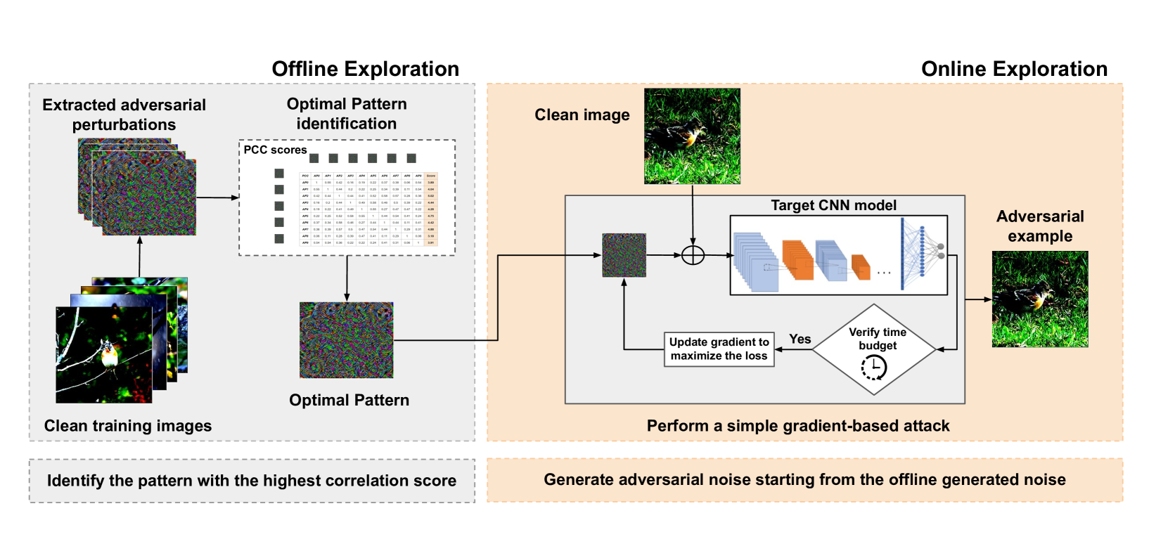
Figure 1: Architecture of the proposed approach: Offline and Online exploration.

In contrast with the existing work on adversarial machine learning, this paper suggests including time as an analysis perspective of adversarial noise generation. More specifically, in addition to the noise budget used in the state-of-the-art, we consider time budget as an orthogonal constraint taken into account in the adversarial noise generation towards more practical threat models and defenses.

To include time as a constraint in the adversarial noise generation process, we first distinguish the time budget from the two design spaces, i.e., online and offline, as follows:

• Online time budget: which we note $T_{on}$, is defined as the time required for the online exploration, i.e., after the acquisition of the victim sample to target.

• Offline time budget: which we note $T_{off}$, is defined as the time required for the offline exploration to generate the adversarial perturbation. During this time, we assume that the attacker has no access to the victim data sample to target.

Hence, we consider the adversarial noise generation as a continuous process combining offline and online processing.

We distinguish the two corner cases mentioned earlier in Section I, where: (i) $(T_{off}=0,T_{on}=\infty)$ corresponds to the conventional digital attack where all the computations are performed online without time limit, and (ii) $(T_{off}=\infty,T_{on}=0)$ corresponds to the universal adversarial perturbation referred to as Offline attack where all the computations are performed offline without time limit.

In this section, we propose real-time Offline-Online Model (ROOM), a new methodology for adversarial noise generation by combining both offline and online exploration under a time constraint. The proposed offline exploration is based on an analysis detailed later in Section V, where we explore the opportunities provided by patterns in adversarial examples that we exploit to warm-up the online exploration instead of starting from random initialization. Figure 1 shows an overview on the proposed methodology and the two phases (offline and online) are detailed in Sections III-B and III-C.

III-B Offline Exploration

The main objective of the offline exploration is to identify the most efficient adversarial noise pattern that corresponds to a static adversarial component on which we can later (during the online exploration) build upon to quickly converge to an adversarial example. Algorithm 1 gives a detailed description of the offline exploration mechanism. To efficiently identify a potential noise pattern, the exploration process implements the following steps: First, we select a set of images for which we generate the corresponding adversarial examples (AEs) and collect adversarial perturbations $P_{i}$ (Line $4$ – $7$ in Algorithm 1). Next, we calculate the correlation between the resulting noise distributions (Line 9 – 13). Subsequently, the aim is to identify the perturbation that has the highest correlation with the other samples, which correspond to the highest intra-class similarity (detailed analysis in Section V). For this reason, we define the similarity score of a given noise as the sum of its PCCs with the remaining noise candidates:

$$\mathcal{S}^{i}_{score}=\sum_{k\neq i}PCC_{i,k}$$

Notice that the higher the similarity score, the closer the noise sample is to the potential static component (adversarial pattern) of the given intra-class setting. In fact, the noise candidate with the maximum $\mathcal{S}_{score}$ represents the highest static component that is redundant within most of the set’s noise samples. Therefore, we finally identify the noise pattern as the noise candidate with the highest similarity score (Line 19–20).

Algorithm 1 Offline Exploration (Optimal noise pattern identification)

1:Input: a classifier $f$, $x$ input image, $y$ true class, $y_{target}$ target class, noise budget $\varepsilon$, $m$ size of the used Set

2:Output: $pattern_{adv}$

3:// Generate AEs and collect $P_{i}$

4:for i = 0 …m-1 do

5:     $x^{*}_{i}=Attack(f,x_{i},y_{i},y_{target},\varepsilon)$

6:     $P_{i}={x^{*}_{i}-x_{i}}$

7:end for

8:// Calculate the correlation between patterns $P_{i}$

9:for s = 0 …m-1 do

10:     for k = 0 …m-1 do

11:         $PCC_{s,k}=corr(P_{s},P_{k})$

12:     end for

13:end for

14:// Set a similarity score for each candidate pattern $P_{i}$ as the sum of PCCs

15:for i = 0 …m-1 do

16:     $\mathcal{S}^{i}_{score}=\sum_{k\neq i}PCC_{i,k}$

17:end for

18:// Identify the $P_{i}$ with the highest correlation score

19:$j=argmax(\mathcal{S}_{score})$

20:$pattern_{adv}=P_{j}$

III-C Online Exploration

After the offline exploration, an adversarial noise pattern is identified as a potential static component that better characterizes the path ”Source–Target” given a decision boundary defined by the trained victim classifier. Our goal is to propose a novel approach for attacking trained models while considering a time budget. Hence, in the quest for a rapid adversarial example generation, the idea is to take advantage of the offline exploration to enhance the online generation efficiency. More specifically, we accelerate the conventional adversarial noise generation approaches with the offline-identified adversarial pattern. Essentially, the perturbation identified from the previous analysis is used as the initial starting point for a new adversarial attack targeting the same class. In fact, the noise pattern is identified such that it represents a static noise component that brings a given input from a source class $l$ closer to a target class $k$. Therefore, instead of starting the exploration of the adversarial noise from a zero or a random matrix, we start the online space exploration from an intermediate point that has a higher chance to be close to the decision boundary, and hence easier to flip the data sample classification to the target label. More importantly, the online exploration becomes faster in producing adversarial examples, allowing it to meet real-time constraints. Algorithm 2 details an illustration of the online exploration where we use the proposed technique to build a Projected Gradient Descent (PGD) based attack where the adversarial example is initialized using the previously generated pattern.

Algorithm 2 Proposed PGD-ROOM attack

1:Input: a classifier $f$ with loss $J$, noise budget $\varepsilon$,step size $\alpha$, $x$ input image, $y_{target}$ targeted class, $pattern_{adv}$ adversarial pattern (identified offline), $m$ number of iterations, $T_{on}$ online time budget

2:Output: $x_{adv}$

3:$begin\_time=time.time()$

4:Initialize  $x_{adv}=pattern_{adv}$

5:for i= 0…m-1 do

6:     if $time.time()-begin\_time>T_{on}$ then

7:         break

8:     end if

9:     prediction = $argmax(f(x_{adv}))$

10:     $x_{adv}=Clip\{x-\varepsilon sign(\nabla_{x_{adv}}J_{\theta}(f(x_{adv}),y_{target}))\}$

11:end for

IV Experiments

In this section, we evaluate the proposed methodology from different perspectives. Precisely, we first assess the offline exploration mechanism to verify the efficiency of the noise pattern identification, especially in terms of adversarial impact. Second, we investigate the behavior of ROOM under both time and noise constraints comparatively with conventional techniques. For thorough investigation, we compare ROOM with both zero and random initialization. Finally, we compare ROOM with a state-of-the-art adversarial training acceleration technique, i.e., YOPO, and show that combining ROOM and YOPO results in even further time efficiency, which offers an interesting property for low-cost adversarial training.

IV-A Setup

Our experiments include implementations of a CNN architecture (Four convolutional layers and three fully connected layers) trained with MNIST [24] for handwritten digit recognition. MNIST is composed of $60,000$ images, with $10$ classes and is composed of grey-scaled images of size $28\times 28$ pixels. We also use Wide ResNet-34 CNN trained on CIFAR-10 database [25] for object recognition in the evaluation. This database consists of 60,000 $32\times 32$ RGB images in $10$ classes, with $6,000$ images per class. Finally, we consider VGG-19 CNN trained on ImageNet [26], which contains over $14$ labeled million images of $224\times 224$ pixels each.

To evaluate the attacks, we used two commonly used adversarial attack generation algorithms, namely: PGD [13] and C&W [11]. The PGD attack is currently the strongest known attack for the $l_{\infty}$ metric. The C&W attack is considered to be one of the strongest $l_{2}$ attacks. Our implementations are built using the open source machine learning framework PyTorch [27]. We modified the FoolBox Library [28] to support our approach and to evaluate the attacks. Experiments were taken on NVIDIA Tesla K80 GPU.

IV-B Evaluation of the offline adversarial pattern exploration

In this section, we evaluate the efficiency of the adversarial noise pattern extraction proposed in Section III-B. For this reason, we use different patterns with different similarity score levels as the exploration initial starting point and monitor the classification accuracy of the model under attack. Specifically, we chose patterns with three similarity score levels: the minimum, the median, and the maximum among the exploration set. Recall that this latter corresponds to our choice of noise pattern when using the offline exploration.

Figures 2 and 3 show that using patterns with higher similarity scores leads to more powerful attacks. In fact, with a perturbation magnitude of $0.2$, we report a model classification accuracy degraded to less than $20\%$ when using the pattern with the highest score, while it remains up to $90\%$ when using the pattern with the lowest score. Changing the size of the exploration set ($m$) used to produce distinct adversarial patterns also reveals that the larger the employed set, the more likely it is to uncover a pattern with a higher similarity score and thereby a higher attack success rate. Notice that the $m$ samples of the considered sets are randomly chosen.

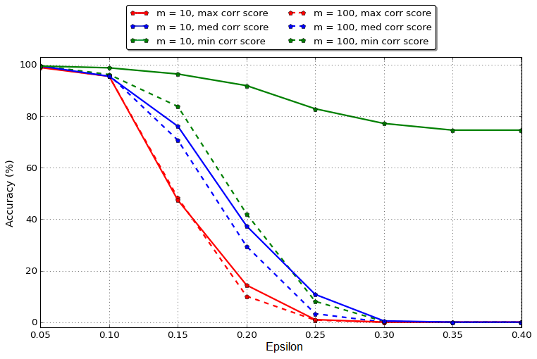
Figure 2: Model classification accuracy under PGD attack when using patterns generated with max, median and min similarity scores for MNIST (m is the exploration Set size)

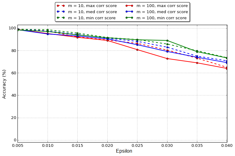
Figure 3: Model classification accuracy under PGD attack when using patterns generated with max, median and min similarity scores for CIFAR-10 (m is the exploration Set size)

IV-C Evaluation under noise and time constraint

In these experiments, we set a time budget for the online processing while varying the noise budget and comparing the performance of the state-of-the-art attacks to ROOM-enhanced version of the attacks.

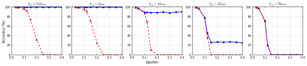
Figure 4: Model classification accuracy under the PGD (blue) and the PGD-ROOM (red) attacks for different time budgets (MNIST).

Attacks on MNIST. To assess the effectiveness of ROOM, we randomly choose four different pairs of (source, target) classes from MNIST test set and generate the optimal adversarial pattern for each to be used as initialization when generating the AE. In Figure 4, we show the model accuracy under ROOM and conventional PGD attack comparatively for different noise budgets $\varepsilon$, and for different time budgets.

We can observe that PGD-ROOM efficiently generates adversarial examples at a maximum throughput of $1250$ FPS under a noise budget of $0.25$. More specifically, ROOM can totally jeopardize the classification accuracy of the victim model processing data streaming in real-time with a speed of $1250$ FPS. However, at the same pace, the conventional online PGD attack was unable to have any impact on model accuracy even for a higher noise budget of $0.4$.

Moreover, for a throughput of $28$ FPS, the victim model misclassifies the totality of samples under ROOM attack, while the baseline attack’s maximum success rate is $75\%$ even for a higher noise budget.

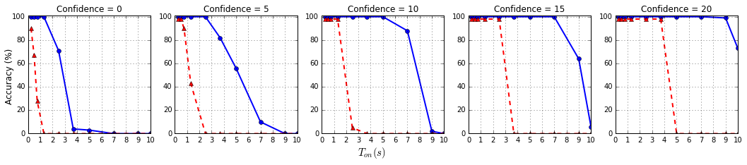
Figure 5: Model classification accuracy under the C&W (blue) and the C&W-ROOM (red) attacks for different time budgets at various confidence levels (MNIST).

In Figure 5, we evaluate the performance of the conventional C&W comparatively to ROOM-C&W. We measure the model accuracy under both attacks while varying the time budget for different confidence levels. Notice that confidence parameter for C&W is the target confidence of the misclassification for an adversarial example. Thus, unlike the PGD attack that crafts adversarial examples within a given perturbation level, C&W finds the smallest perturbation needed to cause misclassification with a given target confidence level. Furthermore, higher confidence requires more time to be reached since it controls the gap between the generated AE and the decision boundary.

For zero-confidence, and with a throughput of $2$ FPS, C&W-ROOM reaches $67\%$ success rate, while the model accuracy remains intact with the conventional attack. The conventional C&W attack requires $5\times$ more time to reach the same performance, which illustrates the effectiveness of our approach.

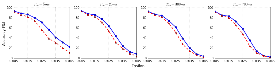
Figure 6: Model classification accuracy under the PGD (blue) and PGD-ROOM (red) attacks for different time budgets (CIFAR-10).

Attacks on CIFAR-10. We generate adversarial examples for images from the CIFAR-10 dataset. Attacking deeper models and larger size and more complex images (RGB) requires a higher time budget. As shown in Figure 6, ROOM outperforms the conventional PGD attack.

For the same target attack success rate of $60\%$ under a noise budget $\varepsilon=0.03$, PGD-ROOM offers a throughput of $200$ FPS, while the maximum throughput of the conventional PGD is only $1.4$ FPS. The same trend was observed for C&W-based attacks: Figure 7 shows clearly that ROOM outperforms the conventional attack. For instance, for a time budget of $10$ seconds, ROOM is $30\%$ more efficient than the conventional C&W. For a confidence equal to $5$, the conventional attack takes $2\times$ more time to reach the same success rate.

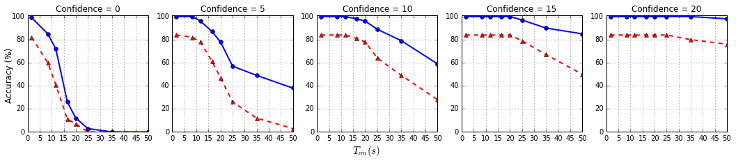
Figure 7: Model classification accuracy under the C&W (blue) and the C&W-ROOM (red) attacks for different time budgets at various confidence levels (CIFAR-10).

Attacks on ImageNet. In this section, we evaluate our approach on the ImageNet dataset. As shown in Figure 8, our proposed PGD-ROOM attack is found to be more effective. PGD-ROOM delivers the same attack success rate of $60\%$ for a throughput of $16$ FPS when the noise budget $\varepsilon=0.025$. However, the conventional attack achieves the same attack effectiveness for a throughput of $0.625$ FPS.

The same trend has been observed for C&W-based attacks, as shown in Figure 9. C&W-ROOM is $15\%$ more effective than the conventional C&W attack for the same allocated time.

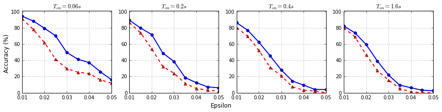
Figure 8: Model classification accuracy under the PGD (blue) and PGD-ROOM (red) attacks for different time budgets (ImageNet).

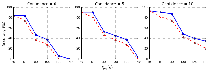
Figure 9: Model classification accuracy under the C&W (blue) and C&W-ROOM (red) attacks for different time budgets at various confidence levels (ImageNet).

IV-D Does ROOM have inherent impact on attack generation?

In this section, our objective is to investigate the impact of the offline exploration from a pure attack efficiency perspective for a given noise budget. We want to answer whether ROOM’s impact is inherent or can be achieved by any random initialization?

For a conclusive evaluation, we explore ROOM comparatively with both zero and random initialization of the adversarial noise. We use PGD with different numbers of steps.

MNIST. We set the size of perturbation as $\varepsilon=0.3$ with a step size of $\frac{8}{255}$. We use PGD with different numbers of iterations and we report the classification accuracy in Table I. We notice that ROOM outperforms all other approaches. For instance, with PGD-10 (PGD with $10$ iterations), ROOM is $3\times$ more powerful than random noise-based attack and more than $6\times$ more powerful than zero noise-based attack.

TABLE I: Model classification accuracy under PGD attack with different initialization methods on MNIST.

Initialization	PGD-40	PGD-10	PGD-5	PGD-3	PGD-2
Zero	1.6%	84.9%	96.8%	98.5%	99.5%
Random	0.2%	47%	89.5%	95.8%	97.1%
ROOM	0%	13.7%	47.7%	69.4%	76.3%

CIFAR-10. We set the size of perturbation as $\varepsilon=0.03$ with a step size of $\frac{2}{255}$. As shown in Table II, using ROOM made the attack more powerful, $1.5\times$ and $1.3\times$ more effective than zero and random noise-based attacks, respectively.

TABLE II: Model classification accuracy under PGD attack with different initialization methods on CIFAR-10.

Initialization	PGD-20	PGD-4	PGD-3	PGD-2	PGD-1
Zero	0%	9.56%	19%	40.87%	71.66%
Random	0%	8.8%	15.2%	32.28%	62.1%
ROOM	0%	6.74%	13.1%	26.53%	48.81%

ImageNet. We use VGG-19 as the classifier for testing ImageNet. The noise magnitude is set to $\varepsilon=0.03$ with step size $\frac{2}{255}$. As illustrated in Table III, using ROOM with PGD attack made the attack more powerful, $1.6\times$ and $1.3\times$ more effective than zero and random noise-based attacks, respectively for PGD-3.

Those results confirm that our offline exploration significantly impacts an attack generation perspective even without considering time constraints. ROOM helps generate more effective adversarial attacks when compared to other initialization methods and for a limited number of attack iterations.

TABLE III: Model classification accuracy under PGD attack with different initialization methods on ImageNet.

Initialization	PGD-20	PGD-5	PGD-3	PGD-1
Zero	0%	15.62%	34.37%	75%
Random	0%	12.5%	28.12%	71.87%
ROOM	0%	8.37%	20.87%	55.62%

IV-E ROOM vs YOPO

In the quest of accelerating the adversarial training process, You Only Propagate Once (YOPO) [29] has been recently proposed. YOPO is based on reducing the total number of full forward and backward propagation to only one for each group of adversary updates by restricting most of the forward and back propagation within the first layer of the network, taking advantage of the baseline training gradient backpropagation. To evaluate our approach comparatively with YOPO, we run experiments where we set a time budget to $0.04$s and $0.08$s for adversarial example generation (corresponding respectively to $25$ and $12$ FPS) and we compare the effectiveness of each attack. Since ROOM is orthogonal to YOPO (YOPO focus on accelerating gradient-based noise generation, while ROOM focuses on noise patch initialization), we also explore the results of combining both techniques.

MNIST. As illustrated in Table IV, PGD-ROOM is more efficient in generating adversarial examples than YOPO initialized with zero and random noise for a throughput of 25 FPS. PGD-ROOM is nearly $6.5\times$ and $2.5\times$ more efficient than YOPO-Zero and YOPO-Random, respectively. Interestingly, we also noticed that combining YOPO with ROOM resulted in more gain in attack success rate.

TABLE IV: Model classification accuracy under ROOM vs YOPO on MNIST for a throughput of 25 FPS.

Attacks	Eps = 0.2	Eps = 0.3
PGD-Zero	52.5%	51.2%
PGD-Random	41.9%	17.6%
PGD-ROOM	23.2%	6.8%
YOPO-Zero	44.8%	44.6%
YOPO-Random	43%	16%
YOPO-ROOM	20.2%	3.7%

CIFAR-10. For a larger model, and a throughput of 12 FPS, we noticed the same trend; ROOM with PGD outperforms YOPO, and combining ROOM and YOPO yields to even better performance. For instance, YOPO-ROOM is more than $2\times$ more powerful than YOPO-random, and PGD-ROOM is $1.4\times$ more successful than YOPO-random.

TABLE V: Model classification accuracy under ROOM vs YOPO on CIFAR-10 for a throughput of 12 FPS.

Attacks	Eps = 0.02	Eps = 0.03
PGD-Zero	37%	30%
PGD-Random	28%	21%
PGD-ROOM	15%	12%
YOPO-Zero	23%	19%
YOPO-Random	20%	17%
YOPO-ROOM	16%	8%

In conclusion, we notice that ROOM generates more effective adversarial attacks than YOPO under the same time constraint, which is a critical metric in scenarios like adversarial training when adversarial examples need to be generated for the whole training set. Moreover, YOPO can be applied only to gradient-based attacks, while ROOM can be integrated into any attack generation method. Interestingly, since ROOM is orthogonal to YOPO, we noticed that combining both techniques results in an even more efficient adversarial example generation. We believe this is a promising property of ROOM to help provide more optimized AML protection.

V How does the offline exploration accelerate adversarial noise generation?

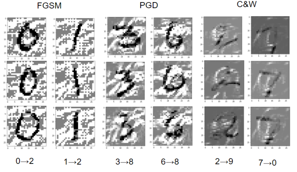
Figure 10: Perturbation distributions samples under different targeted adversarial attacks on MNIST.

In this section, we investigate the spatial patterns of adversarial noise in image recognition applications. Conceptually, we explore if the noise resulting from pushing a given example towards the decision boundary contains a specific spatial pattern. This study provides the basis for the idea of splitting noise generation between offline and online phases towards a generic perspective of adversarial noise generation under noise and time constraints.

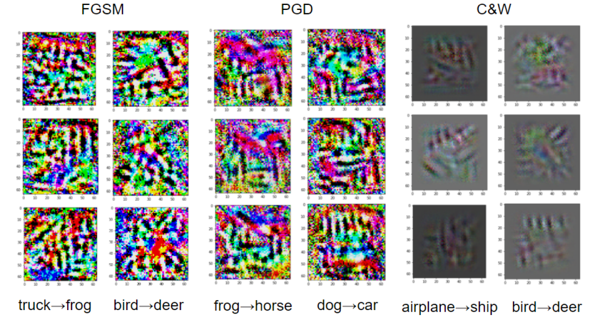
Figure 11: Perturbation distributions samples under different targeted adversarial attacks on CIFAR-10.

First, we consider samples belonging to the same initial class on which we generate targeted adversarial noise towards a fixed target class. The objective is to explore the existence of potential spatial patterns in the noise distributions generated by adversarial attacks. An illustration of noise examples for different targeted attacks on MNIST and CIFAR-10 datasets are shown in Figures 10 and 11, respectively. The illustrations show that a general pattern between pairs of classes could be extracted from the resulting adversarial noise. For MNIST dataset, since the data is relatively simple, we could see clear patterns for targeted adversarial attacks with plausible semantics; Attacking these pixels will alter the original handwriting shape towards the target class’s shape. For the CIFAR-10 dataset, since the images have three channels (RGB), the noise is not easily interpretable, yet, patterns can be identified for the same targeted attacks.

To further assess the generalizability of this observation, we perform a statistical study on the similarity of generated noise within the same target and compare its distribution to adversarial noise for different targets. To assess this noise matrix similarity, we use the Pearson correlation coefficient (PCC) [30], which is a widely adopted metric to measure the linear correlation between two variables.

PCC coefficient is defined as follows:

$$PCC_{X,Y}=\frac{cov(X,Y)}{\sigma_{X}\sigma_{Y}}$$ (9)

where $cov$ indicates the covariance and $\sigma_{X}$ and $\sigma_{Y}$ are the standard deviations of matrices $X$ and $Y$, respectively, and the $PCC$ values range from $-1$ to $1$. The absolute value indicates the extent to which the two variables are linearly correlated, with $1$ indicating perfect linear correlation, $0$ indicating zero linear correlation, and the sign indicates whether they are positively or negatively correlated.

The targeted adversarial noise is iteratively constructed to transform a sample from a source class (correct label) towards an adversarial sample $x^{*}_{i}$ with a target class (target misclassification label). This transformation path has naturally higher similarity for noise generated on samples from the same source targeting the same class, compared to noise generated on samples belonging to different pair (source,target) classes. Therefore, our intuition is that a static noise component could be present in high-dimensional space among the samples from a given class in the path towards a specific target class given a decision boundary.

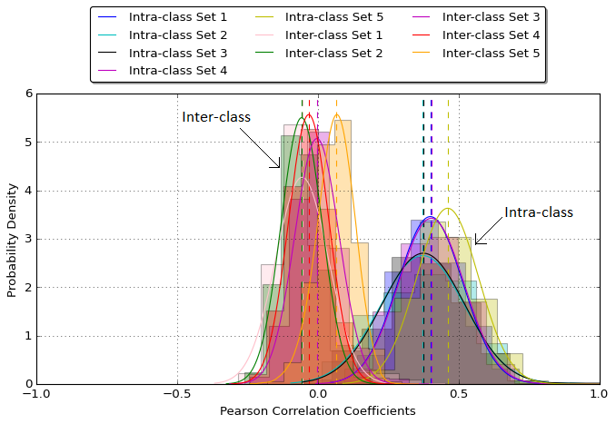
Figure 12: Gaussian distribution of Pearson correlation coefficients PGD MNIST intra-class vs inter-class.

We analyze the similarities between noise distributions within a given setting (source,target), which we call intra-class similarity, comparatively with the distribution of noise similarities between two different settings (source,target), which we call inter-class similarity.

Let $x_{i}$ be an input sample and $f$ a given classifier such that $f(x_{i})=l$. Let be a targeted adversarial attack that generates an adversarial noise defined as:

$$\varepsilon^{lk}_{i}~{}.s.t.~{}f(x_{i}+\varepsilon^{lk}_{i})=k\neq l$$ (10)

Let ${S}_{ij}$ be the similarity between two noises $\varepsilon^{lk}_{i}$ and $\varepsilon^{pq}_{j}$ for two samples $x_{i}$ and $x_{j}$, respectively, defined as follows:

$$\mathcal{S}_{ij}=PCC(\varepsilon^{lk}_{i},\varepsilon^{pq}_{j})$$ (11)

Where PCC is the Pearson correlation coefficient [30], used as a similarity metric. We call $\mathcal{S}_{ij}$ an inter-class similarity when $(p,q)\neq(l,k)$, and we call $\mathcal{S}_{ij}$ an intra-class similarity when $(p,q)=(l,k)$.

In Figures 12, 13 and 14, we represent the distribution of different measured similarity $\mathcal{S}_{ij}$ values for MNIST, CIFAR-10 and ImageNet datasets, respectively. We notice that the intra-class similarity distribution is clearly higher than the inter-class similarity distribution for the three datasets. This observation supports our intuition of the presence of patterns for the same (source, target) setting of adversarial noise. It, therefore, explains the mechanism by which an offline exploration allows to converge more quickly to an adversarial example.

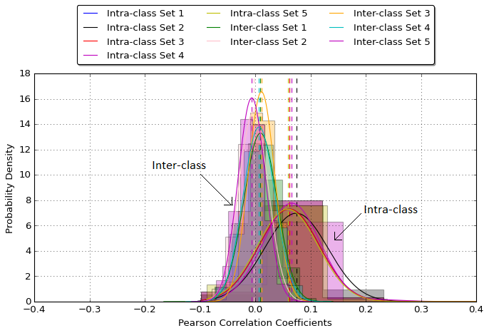
Figure 13: Gaussian distribution of Pearson correlation coefficients PGD cifar-10 intra-class vs inter-class.

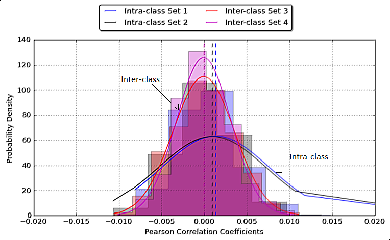
Figure 14: Gaussian distribution of Pearson correlation coefficients PGD ImageNet intra-class vs inter-class.

VI Discussion

For the first time, this paper introduces a new problem of crafting effective AML attacks under time constraints. From a run-time perspective, existing state-of-the-art methods represent two ends of the spectrum: fully offline universal attacks and fully online input-specific attacks. To show the continuum over time of adversarial attack generation problem, we propose a new adversarial noise generation method, ROOM, that bridges the two AML approaches in the quest of fast generation of input-specific adversarial perturbations. Specifically, ROOM uses an offline-generated noise pattern, specialized for the current input, to warm up the online component of the attack. As a result, the online exploration can rapidly converge towards a successful attack by starting from this offline-generated specialized static noise, making input-specific attacks much faster. We show that for the same time budget, ROOM substantially outperforms state-of-the-art adversarial attack methods. In fact, for the same attack success rate, ROOM converges to an adversarial example up to $5$ times and $12$ times faster on average than C&W [11] and PGD [13] attacks, respectively. Importantly, ROOM can meet real-time constraints for a camera streaming with $25$ frames per second, generating adversarial examples at a matching rate. In fact, for a noise budget of $0.035$ and a time budget of $0.03$ seconds, ROOM achieves up to $85\%$ attack success rate, at $25$ fps throughput.

We believe that ROOM is an important step towards producing adversarial attacks that can be deployed just-in-time. Just-in-time attacks can be a game-changer in the adversarial attacks threat model since it makes it possible for malicious actors to deploy adversarial attacks opportunistically based on the state of the environment. Additionally, these attacks are highly challenging to protect from, especially for real-time applications and Cyber-Physical Systems. Therefore, the community needs to understand the attacker’s capability, which we advance using ROOM attacks.

From another perspective, we showed that ROOM can be combined with YOPO, which is dedicated to accelerating adversarial training. This is due to ROOM’s orthogonal property to gradient-based methods, and hence could be used for a more time-efficient adversarial training.

ROOM is a general pattern of attack relying on the offline component to create a more favorable initial state for the online exploration. We presented example implementations of the offline component that we believe can still be substantially improved. Moreover, we believe that additional optimization opportunities remain, including the use of hardware acceleration. Finally, we would also like to explore whether the ROOM strategy results in different opportunities for defenders because of the resulting noise distribution, which is likely to be different from online only attacks. Our future work will also explore ROOM on different learning structures and applications such as audio/NLP processing.

VII Related work

State-of-the-art adversarial attacks such as PGD [13], and C&W [11] are found to be effective in fooling DNNs. However, these attacks rely on time-consuming iterative optimization approaches, making them too slow to be launched against real-time systems. These methods are based on the assumption of an infinite online time budget. The attacker has access to the entire data sample with a single constraint on the noise magnitude, which is not suitable for real-life situations.

Universal adversarial perturbations [31] are based on generating an adversarial perturbation patch that works for a variety of samples. The universal adversarial perturbation is fully created offline and does not use real-time observations to improve efficiency for a target data sample. This substantially limits their efficiency.

One of the preliminary works that studied dynamic real-time adversarial attacks was [22], where a real-time adversarial attack for models with streaming inputs is proposed. In this scenario, an attacker can only view previous portions of the data sample and only introduce perturbations to future portions of the data sample, whereas the target model’s decision will be predicated based on the entire data sample. The generated noise uses imitation learning and behavioral cloning algorithm to train real-time adversarial perturbation generator through non-real-time adversarial perturbation generator.

Li et al. [21] use deep reinforcement learning to generate periodic adversarial perturbations to attack a recurrent neural network processing sequential data. The attack is used to generate adversarial perturbations to fool the DeepSpeech Speech Recognition system. Z. Li et al. [32] proposed AdvPulse: a penalty-based universal adversarial perturbation generation approach that incorporates the varying time into the optimization process to get around the constraints on speech content and time. Another work [33] proposed a fast audio adversarial perturbation generator (FAPG), which uses a generative model to generate adversarial perturbations for the audio input in a single forward pass. However, this method is unpractical since the propagation time would be lower than the generative model delay added to the generated adversarial noise propagation delay.

VIII Conclusions

This paper contributes a new perspective of generating and analyzing adversarial attacks by introducing a real-time constraint. We present a novel real-time online-offline attack model (ROOM) to rapidly generate adversarial attacks suitable for use in just-in-time attack settings. ROOM leverages an offline component to support the online algorithm, allowing for rapid convergence to highly successful attacks. Our results show that using an offline adversarial pattern as a starting point for the online exploration accelerated conventional adversarial attacks. For instance, our proposed PGD-based attack achieves a $100\%$ attack success rate for a noise budget of $0.25$ under $0.0008$ seconds time constraint, whereas, for the same allocated runtime, the conventional attack is unable to generate any successful adversarial example, even for a higher noise ($0.4$) for MNIST database.

References

- [1] K. Simonyan and A. Zisserman, “Very deep convolutional networks for large-scale image recognition,” 2014.
- [2] J. Redmon and A. Farhadi, “Yolo9000: Better, faster, stronger,” 2016.
- [3] L. Deng and Y. Liu, Deep learning in natural language processing. Springer, 2018.
- [4] H. A. Pierson and M. S. Gashler, “Deep learning in robotics: a review of recent research,” Advanced Robotics, vol. 31, no. 16, pp. 821–835, 2017.
- [5] M. Al-Qizwini, I. Barjasteh, H. Al-Qassab, and H. Radha, “Deep learning algorithm for autonomous driving using googlenet,” in 2017 IEEE Intelligent Vehicles Symposium (IV). IEEE, 2017, pp. 89–96.
- [6] R. Miotto, F. Wang, S. Wang, X. Jiang, and J. T. Dudley, “Deep learning for healthcare: review, opportunities and challenges,” Briefings in bioinformatics, vol. 19, no. 6, pp. 1236–1246, 2018.
- [7] F. Tramèr, F. Zhang, A. Juels, M. K. Reiter, and T. Ristenpart, “Stealing machine learning models via prediction apis,” in 25th USENIX Security Symposium (USENIX Security 16). Austin, TX: USENIX Association, Aug. 2016, pp. 601–618. [Online]. Available: https://www.usenix.org/conference/usenixsecurity16/technical-sessions/presentation/tramer
- [8] N. Papernot, P. McDaniel, and I. Goodfellow, “Transferability in machine learning: from phenomena to black-box attacks using adversarial samples,” 2016.
- [9] I. J. Goodfellow, J. Shlens, and C. Szegedy, “Explaining and harnessing adversarial examples,” 2014.
- [10] A. Kurakin, I. J. Goodfellow, and S. Bengio, “Adversarial examples in the physical world,” CoRR, vol. abs/1607.02533, 2016. [Online]. Available: http://arxiv.org/abs/1607.02533
- [11] N. Carlini and D. A. Wagner, “Towards evaluating the robustness of neural networks,” CoRR, vol. abs/1608.04644, 2016. [Online]. Available: http://arxiv.org/abs/1608.04644
- [12] N. Carlini, A. Athalye, N. Papernot, W. Brendel, J. Rauber, D. Tsipras, I. Goodfellow, A. Madry, and A. Kurakin, “On evaluating adversarial robustness,” 2019.
- [13] A. Madry, A. Makelov, L. Schmidt, D. Tsipras, and A. Vladu, “Towards deep learning models resistant to adversarial attacks,” 2017.
- [14] N. Carlini and D. A. Wagner, “Adversarial examples are not easily detected: Bypassing ten detection methods,” CoRR, vol. abs/1705.07263, 2017. [Online]. Available: http://arxiv.org/abs/1705.07263
- [15] N. Papernot, P. McDaniel, X. Wu, S. Jha, and A. Swami, “Distillation as a defense to adversarial perturbations against deep neural networks,” in 2016 IEEE Symposium on Security and Privacy (SP), May 2016, pp. 582–597.
- [16] T. Chavdarova, P. Baqué, S. Bouquet, A. Maksai, C. Jose, T. Bagautdinov, L. Lettry, P. Fua, L. Van Gool, and F. Fleuret, “Wildtrack: A multi-camera hd dataset for dense unscripted pedestrian detection,” in 2018 IEEE/CVF Conference on Computer Vision and Pattern Recognition, 2018.
- [17] A. Ben Khalifa, I. Alouani, M. A. Mahjoub, and A. Rivenq, “A novel multi-view pedestrian detection database for collaborative intelligent transportation systems,” Future Generation Computer Systems, vol. 113, pp. 506–527, 2020.
- [18] S. Thys, W. V. Ranst, and T. Goedemé, “Fooling automated surveillance cameras: Adversarial patches to attack person detection,” in 2019 IEEE/CVF Conference on Computer Vision and Pattern Recognition Workshops (CVPRW), 2019, pp. 49–55.
- [19] X. Liu, H. Yang, Z. Liu, L. Song, H. Li, and Y. Chen, “Dpatch: An adversarial patch attack on object detectors,” 2019.
- [20] D. Karmon, D. Zoran, and Y. Goldberg, “LaVAN: Localized and visible adversarial noise,” in Proceedings of the 35th International Conference on Machine Learning, ser. Proceedings of Machine Learning Research, vol. 80. PMLR, 2018.
- [21] C. R. Serrano, P. Sylla, S. Gao, and M. A. Warren, “Rta3: A real time adversarial attack on recurrent neural networks,” in 2020 IEEE Security and Privacy Workshops (SPW), 2020, pp. 27–33.
- [22] Y. Gong, B. Li, C. Poellabauer, and Y. Shi, “Real-time adversarial attacks,” ArXiv, vol. abs/1905.13399, 2019.
- [23] X. Yuan, P. He, Q. Zhu, R. R. Bhat, and X. Li, “Adversarial examples: Attacks and defenses for deep learning,” CoRR, vol. abs/1712.07107, 2017. [Online]. Available: http://arxiv.org/abs/1712.07107
- [24] Y. LeCun and C. Cortes, “MNIST handwritten digit database,” 2010. [Online]. Available: http://yann.lecun.com/exdb/mnist/
- [25] A. Krizhevsky, “Learning multiple layers of features from tiny images,” Tech. Rep., 2009.
- [26] J. Deng, W. Dong, R. Socher, L.-J. Li, K. Li, and L. Fei-Fei, “ImageNet: A Large-Scale Hierarchical Image Database,” in CVPR09, 2009.
- [27] A. Paszke, S. Gross, F. Massa, A. Lerer, J. Bradbury, G. Chanan, T. Killeen, Z. Lin, N. Gimelshein, L. Antiga, A. Desmaison, A. Köpf, E. Yang, Z. DeVito, M. Raison, A. Tejani, S. Chilamkurthy, B. Steiner, L. Fang, J. Bai, and S. Chintala, “Pytorch: An imperative style, high-performance deep learning library,” 2019.
- [28] J. Rauber, W. Brendel, and M. Bethge, “Foolbox v0.8.0: A python toolbox to benchmark the robustness of machine learning models,” CoRR, vol. abs/1707.04131, 2017. [Online]. Available: http://arxiv.org/abs/1707.04131
- [29] D. Zhang, T. Zhang, Y. Lu, Z. Zhu, and B. Dong, “You only propagate once: Accelerating adversarial training via maximal principle,” 2019.
- [30] T. Anderson, “An introduction to multivariate statistical analysis (wiley series in probability and statistics),” 2003.
- [31] S. Moosavi-Dezfooli, A. Fawzi, O. Fawzi, and P. Frossard, “Universal adversarial perturbations,” in 2017 IEEE Conference on Computer Vision and Pattern Recognition (CVPR), 2017, pp. 86–94.
- [32] Z. Li, Y. Wu, J. Liu, Y. Chen, and B. Yuan, “Advpulse: Universal, synchronization-free, and targeted audio adversarial attacks via subsecond perturbations,” in Proceedings of the 2020 ACM SIGSAC Conference on Computer and Communications Security, ser. CCS ’20. New York, NY, USA: Association for Computing Machinery, 2020, p. 1121–1134. [Online]. Available: https://doi.org/10.1145/3372297.3423348
- [33] Y. Xie, Z. Li, C. Shi, J. Liu, Y. Chen, and B. Yuan, “Enabling fast and universal audio adversarial attack using generative model,” 2021.