Deep Probabilistic Graph Matching

Abstract

Most previous learning-based graph matching algorithms solve the quadratic assignment problem (QAP) by dropping one or more of the matching constraints and adopting a relaxed assignment solver to obtain sub-optimal correspondences. Such relaxation may actually weaken the original graph matching problem, and in turn hurt the matching performance. In this paper we propose a deep learning-based graph matching framework that works for the original QAP without compromising on the matching constraints. In particular, we design an affinity-assignment prediction network to jointly learn the pairwise affinity and estimate the node assignments, and we then develop a differentiable solver inspired by the probabilistic perspective of the pairwise affinities. Aiming to obtain better matching results, the probabilistic solver refines the estimated assignments in an iterative manner to impose both discrete and one-to-one matching constraints. The proposed method is evaluated on three popularly tested benchmarks (Pascal VOC, Willow Object and SPair-71k), and it outperforms all previous state-of-the-arts on all benchmarks.

1 Introduction

Generally speaking, the problem of graph matching aims to find the optimal vertex correspondences between given graphs under structure constraints of keeping the edge consistency. It has been widely used in many applications such as object tracking [1, 2], person re-identification [3], point correspondence[4], etc. Graph matching is in general NP-hard due to its combinatorial nature, and it is thus hard to search a global optimal solution for graphs with large sizes. Therefore, many approximate approaches [5, 6, 7, 8, 9, 10, 11, 12, 13, 14] have been devoted to seeking acceptable suboptimal solutions by relaxing the quadratic assignment problem to a simpler form.

Aiming to improve the matching accuracy in real-world matching tasks, some early efforts [15, 16] have been devoted to learning reasonable affinity measures or adaptive graph representations using the machine learning strategies. However, the improvements are limited because of the shallow parameter settings, and thus still insufficient to handle various challenges.

Recently, approaches [17, 18, 19, 20, 21, 22, 23, 24] based on deep neural networks have attracted much research attention due to the ability to learn representative embeddings of nodes and/or edges. It is common for these approaches to embed a differentiable solver for the combinatorial optimization problem into an end-to-end learning framework. Different from the well-designed combinatorial solvers in previous learning-free graph matching methods, these learning-based methods usually acquire node correspondences in a more straightforward way by relaxing one or more of the quadratic constraints, discrete constraints and one-to-one matching constraints. Examples include [23, 21, 18] that relax the quadratic assignment problem to a node-wise assignment problem and adopt the Sinkhorn algorithm [25] for the optimization of linear assignment, [17] that works directly on the learned pairwise affinities using a spectral matching algorithm [9] but drops both discrete and one-to-one matching constraints, and [22] that relaxes the graph matching problem based on Lagrangian decomposition and employs dual block coordinate ascent implementations for optimization. Despite remarkable performance gained, these relaxations of the original problem may cause potential limitations on matching performance.

To address the issues mentioned above, we propose a novel deep probabilistic graph matching (DPGM) algorithm, which works directly on the learned pairwise affinities and imposes both discrete and one-to-one matching constraints on the matching solutions. Firstly, we design an affinity-assignment prediction network (AA-predictor) to jointly learn the pairwise affinities and the node assignments. Specifically, the AA-predictor performs graph propagation using several delicately designed convolution operators on a constructed affinity-assignment graph (AA-graph), in which each node corresponds to a candidate match and each edge relates to the pairwise affinity between two matches. Subsequently, the learned affinities and estimated assignments of the AA-predictor are passed as inputs to a differentiable probabilistic solver, which refines the estimated assignments in an iterative manner and imposes both discrete and one-to-one matching constraints in a probabilistic way. Finally, the balanced entropy loss between the output matching solutions and ground-truth matches is employed as the supervision signal to guide the training of our framework.

For evaluating the proposed DPGM algorithm, we report its matching performance on three public benchmarks, namely Willow Objects [16], Pascal VOC Keypoints [26] and SPair-71k [27], in comparison with several state-of-the-art graph matching approaches. In experiments our method outperforms all compared methods on all three benchmarks, which illustrates the effectiveness and adaptability of the proposed method in different scenarios. We will release our code publicly available once the paper is accepted.

In summary, with the proposed learning framework for graph matching, this paper makes contribution in three-fold:

1. the proposed differentiable probabilistic solver works directly on the learned pairwise affinities in a probabilistic way, which is expected to be more effective by avoiding the compromise on the matching constraints;

2. unlike most previous graph matching methods that use a trivial guess of an initial assignment for the combinatorial solver, ours learns jointly the pairwise affinities and the initial assignment, which remarkably benefits the final solution (see Tables VI, VII, VIII); and

3. extensive experiments are conducted on three popular benchmarks, in comparison with many state-of-the-art methods, to validate the effectiveness of the proposed method.

2 Related Works

Graph matching has been investigated for decades and many algorithms have been proposed. In this section we review recent learning-based studies or those closely related to ours, and leave general graph matching research to three comprehensive surveys [28, 29, 30].

Aiming to cooperate with the data derived from real-world matching tasks, many learning-based graph matching algorithms, including unsupervised [31], semi-supervised [32] and supervised ones [15, 33], have been proposed to learn the parameters of affinity measure to replace the handcrafted affinity metric. In addition, instead of learning the affinity measure, Cho et al. [16] propose a learnable framework to parameterize the graph model and generate reasonable structural attributes for visual object matching. However, these methods employ simple and shallow parametric models to control geometric affinities between pairs of matches, and the promotion to the matching accuracy is still limited.

With the growing interest in utilizing deep neural network for structured data [34, 35], learning graph matching with graph neural network (GNN) has attracted much research attention. A classic way is to learn representative node and/or edge embeddings via graph neural networks and then relax the graph matching problem to the linear assignment problem. Nowak et al. [36] introduce a Siamese GNN encoder to produce a normalized node embedding for each graph to be matched, and then predict a matching by minimizing the cosine distance between matching pairs of embeddings dictated by the target permutation. Wang et al. [18] employ the graph convolutional network (GCN) framework [37] to produce node embeddings by aggregating graph structure information, and adopt the Sinkhorn network [25] as the combinatorial solver for the relaxed linear assignment problem. SuperGlue [21] is designed for generating discriminative node representations using intra-graph and cross-graph attention, where spatial relationships and visual information are jointly taken into considerations during the node embedding process. In addition, to drop the outlier candidate matches that usually occur in real-world matching tasks, this framework augments each node set with a dustbin so that the unmatched nodes are explicitly assigned to it. To further improve the robustness of learnable affinities, Yu et al. [24] propose a node and edge embedding strategy that simulates the multi-head strategy in attention models, enabling the information in each channel to be merged independently. Fey et al. [23] propose to start from an initial ranking of soft correspondences between nodes, and iteratively refine the solution by synchronous message passing networks to reach neighborhood consensus between node pairs without any optimization inference.

Different from the above mentioned methods that focus mainly on the learning of node and/or edge embeddings and relax the quadratic matching constraints, several recently proposed methods work directly on pairwise affinities and embed differentiable solvers for quadratic optimization. Zanfir et al. [17] formulate graph matching as a quadratic assignment problem under both unary and pairwise affinities, and adopt a spectral matching algorithm [9] as the combinatorial solver that drops both discrete and one-to-one matching constraints in optimization. Rolínek et al. [22] relax the graph matching problem based on Lagrangian decomposition, which is solved by embedding BlackBox implementations of a heavily optimized solver [38] based on dual block coordinate ascent. Reformulating graph matching as Koopmans-Beckmann’s QAP [39] to minimize the adjacency discrepancy of graphs to be matched, Gao et al. [20] adopt the Frank-Wolf algorithm [40] to obtain approximate solutions. Besides, Wang et al. [19] integrate learning of affinities and solving for combinatorial optimization into a unified node labeling pipeline, where the quadratic assignment problem of graph matching has been transformed to the binary classification problem of finding the positive node in a constructed assignment graph.

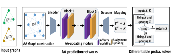
Figure 1: The overview pipeline of the proposed DPGM framework. Taking the two graphs $\mathbb{G}^{(1)}$ and $\mathbb{G}^{(2)}$ to be matched as input, the AA-predictor firstly generates an affinity-assignment graph (AA-graph) $\mathbb{G}^{A}$, where the candidate matches and pairwise affinities are modeled as nodes and edges respectively. Subsequently, the graph state is iteratively updated by the AA-updating module to form structured representations, and it is finally read out by the decoder that maps representations of nodes and edges to entries of the assignment matrix and the pairwise affinity matrix respectively. Finally, the differentiable probabilistic solver starts from the assignments estimated by the AA-predictor, and refines them alternatively by solving QAP in a probabilistic way to obtain better matching solutions.

3 Graph Matching

3.1 Problem formulation

In graph theory, an attributed graph of $n$ nodes can be represented by $\mathbb{G}=\{\mathbb{V},\mathbb{E},\mathcal{V},\mathcal{E}\}$, where $\mathbb{V}=\{v_{1},...,v_{n}\}$ and $\mathbb{E}\subseteq\mathbb{V}\times{\mathbb{V}}$ denote respectively the node set and edge set, and $\mathcal{V}=\{\textbf{v}_{i}|\textbf{v}_{i}\in\mathbb{R}^{d_{V}},i=1,2,...,n\}$ and $\mathcal{E}=\{\textbf{e}_{i}|\textbf{e}_{i}\in\mathbb{R}^{d_{E}},i=1,2,...,|\mathcal{E}|\}$ the node attribute set and edge attribute set, respectively. The node relations in the graph can be represented by a symmetric adjacency matrix $A\in\{0,1\}^{n\times{n}}$, where $A_{ij}=1$ if and only if there is an edge between nodes $v_{i}$ and $v_{j}$.

Given two graphs $\mathbb{G}^{(i)}=\{\mathbb{V}^{(i)},\mathbb{E}^{(i)},\mathcal{V}^{(i)},\mathcal{E}^{(i)}\}$ of size $n$, $i=1,2$, graph matching aims to find node correspondence $X\in\{0,1\}^{n\times{n}}$ between $\mathbb{G}^{(1)}$ and $\mathbb{G}^{(2)}$ that maximizes the global consistency designed as

$$\mathcal{H}=\sum_{i,a}c_{ia}X_{ia}+\sum_{i,j,a,b}d_{ia,jb}X_{ia}X_{jb},$$ (1)

where $c_{ia}$ measures the similarity between node $v_{i}^{(1)}$ in $\mathbb{G}^{(1)}$ and node $v_{a}^{(2)}$ in $\mathbb{G}^{(2)}$, while $d_{ia,jb}$ measures the agreement between edge $(v_{i}^{(1)},v_{j}^{(1)})$ in $\mathbb{G}^{(1)}$ and edge $(v_{a}^{(2)},v_{b}^{(2)})$ in $\mathbb{G}^{(2)}$. The correspondence matrix $X$ indicates the matching results, i.e., $X_{ia}=1$ if and only if $i^{th}$ node of $\mathbb{G}^{(1)}$ matches to $a^{th}$ node of $\mathbb{G}^{(2)}$. In addition, the distribute of $X$ is restricted under the one-to-one matching constraints: $X\textbf{1}_{n}=\textbf{1}_{n}$ and $X^{T}\textbf{1}_{n}=\textbf{1}_{n}$, where $\textbf{1}_{n}$ denotes a $n-$demension one-value vector.

Seeking the optimal solution maximizing the Eq. 1 can be reformulated as a quadratic assignment problem:

$$\textbf{x}^{\ast}=\arg\max_{\textbf{x}}\textbf{x}^{T}K\textbf{x},$$ (2)

where x is the vectorization of $X$, and $K$ the affinity matrix encoding the node similarity and edge agreement at diagonal elements and off-diagonal elements, respectively. In more detail, the affinity matrix $K$ can be expressed as

$$K_{ia,jb}=\left\{\begin{array}[]{ll}c_{ia}&{\rm if~{}~{}}i=j{\rm~{}~{}and~{}~{}}a=b,\\ d_{ia,jb}&{\rm else~{}if~{}~{}}A_{ia}^{(1)}A_{jb}^{(2)}>0,\\ 0&{\rm otherwise.}\end{array}\right.$$ (3)

Note that, for simplicity we assume that the two given graphs to be matched have the same size $n$ in this work, yet this formulation of graph matching can be easily extended to general cases with different sizes by auxiliary strategies, such as adding dummy nodes.

Recently, many efforts have been devoted to improving graph matching accuracy with the combination of deep learning architecture and differentiable relaxation-based solvers. The graph matching problem has been relaxed to a linear assignment problem by learning the high-order node embeddings in [18, 23, 24], and the Sinkhorn algorithm [41] is applied as a combinatorial solver in these works. In [17], the unary and pair-wise affinities are generated by learning deep node and edge representations, and the quadratic assignment problem is solved by a relaxation manner, i.e., spectral matching [9]. A more advanced method has been proposed by Rolínek et al. [22] who propose using strong feature extraction with SplineCNN [42] and leverage the combinatorial solver based on dual block coordinate ascent for Lagrange decompositions [38]. Despite the demonstrated power of deep networks in representation learning, the relaxation strategy applied to graph matching problem is a weakening of the quadratic assignment problem, which may hurt the performance of graph matching.

Unlike the deep graph matching methods discussed above, we treat the graph matching problem as a quadratic assignment problem faithfully without compromise on matching constraints, and solve the problem using a probabilistic optimization scheme that takes as input the estimated affinities and assignments, both of which are jointly learnt through a novel graph information propagation module, and refines the assignment solutions in an iterative manner.

4 The Proposed Method

Our model consists of two core parts: an affinity-assignment prediction network (AA-predictor) and a differentiable probabilistic solver. As illustrated in Fig. 1, the AA-predictor first models the pairwise affinity and candidate matches into a unified affinity-assignment graph (AA-graph), and then performs graph propagation to form the structural representations for nodes and edges, both of which are decoded as the initial assignments and affinities, respectively. Subsequently, the differentiable probabilistic solver takes the estimated assignments and affinities as input, and refines them in a probabilistic manner to obtain the optimal matching solutions.

4.1 Affinity-assignment prediction network

As illustrated in Fig. 1, the AA-predictor takes two graphs to be matched as input, and learns pairwise affinities and candidate assignments through three components including the AA-graph construction, AA-updating module and AA-decoder.

Affinity-assignment graph construction: Given two input graphs $\mathbb{G}^{(1)}$ and $\mathbb{G}^{(2)}$, we model the candidate matches and the pairwise affinities into a so-called affinity-assignment graph (AA-graph) $\mathbb{G}^{A}=\{\mathbb{V}^{A},\mathbb{E}^{A},\mathcal{V}^{A},\mathcal{E}^{A}\}$, where the candidate match between $v_{i}^{(1)}\in\mathbb{V}^{(1)}$ and $v_{a}^{(2)}\in\mathbb{V}^{(2)}$ is denoted as a node $v_{ia}^{A}\in\mathbb{V}^{A}$, and the pair-wise affinity between a pair of candidate matches $v_{ia}^{A},v_{jb}^{A}\in\mathbb{V}^{A}$ is represented by the edge $e_{(ia,jb)}^{A}\in\mathbb{E}^{A}$ if and only if there are two edges $(v_{i}^{(1)},v_{j}^{(1)})\in\mathbb{E}^{(1)}$ and $(v_{a}^{(2)},v_{b}^{(2)})\in\mathbb{E}^{(2)}$.

Fig. 2 illustrates an example of constructing the AA-graph where the candidate matches $X_{1a}$ and $X_{2b}$ are encoded as the nodes $v_{1a}^{A}$ and $v_{2b}^{A}$ in $\mathbb{V}^{A}$ respectively, and the affinity between them (i.e., $K_{1a,2b}$) is modeled into the edge $(v_{1a}^{A},v_{2b}^{A})\in\mathbb{E}^{A}$. Different from the method proposed in [19] that utilizes only geometric cues to form the attributes of nodes and edges, we combine the visual features and geometric information to generate the initial attributes on AA-graph. Specifically, we take the visual features extracted from images by CNNs [43] as the raw node attributes, and concatenate the point coordinates of two nodes associated with the same edge to form the edge attributes as

$$\textbf{v}_{ia}^{A} =[\textbf{f}_{i}^{(1)};\textbf{f}_{a}^{(2)}];$$ (4)

$$\textbf{e}_{(ia,jb)}^{A} =[\textbf{p}_{i}^{(1)};\textbf{p}_{j}^{(1)};\textbf{p}_{a}^{(2)};\textbf{p}_{b}^{(2)}],$$

where $\textbf{f}_{i}^{(1)}$ and $\textbf{p}_{i}^{(1)}$ denote the visual feature and coordinates of the $i^{th}$ keypoint in the $1^{st}$ image respectively, and $[\cdot;\ldots;\cdot]$ concatenates its input along the channel direction.

In this way, the affinity matrix and matches in Eq. 2 have been transformed into high-order representations in the unified AA-graph, and they are alternatively updated to form structured representations by the following AA-updating module.

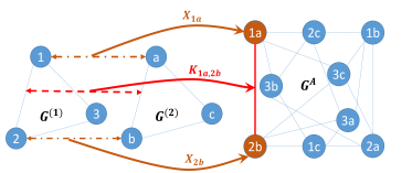
Figure 2: An example of the AA-graph construction.

AA-updating module: This module performs graph propagation by extending the graph network block [19] module to fit our framework. Specifically, this module firstly transforms the original node attributes and edge attributes of the input AA-graph into two latent embedding spaces, and then iteratively updates the affinities (edge attributes) and the assignments (node attributes) by stacking multiple affinity updating layers and assignment updating layers.

For the original AA-graph, the AA-updating module employs the encoder to transform the AA-graph state into latent embedding space as

$$\mathbb{G}^{A}\leftarrow Encoder(\mathbb{G}^{A})=\{\mathbb{V}^{A},\mathbb{E}^{A},\rho_{v}(\mathcal{V}^{A}),\rho_{e}(\mathcal{E}^{A})\},$$ (5)

where $\rho^{v}$ and $\rho^{e}$ are the learnable transformation functions that map the original attributes of nodes and edges into the latent spaces with dimensions of $d_{V}$ and $d_{E}$, respectively. Furthermore, both $\rho_{v}$ and $\rho_{e}$ are designed as two Multi-Layer Perceptrons (MLPs), but with different parameters. After that, the AA-updating module performs graph propagation to form the structural representations for nodes and edges.

Since a pairwise affinity $\textbf{e}_{(ia,jb)}^{A}$ is directly related to its associated matches $\textbf{v}_{ia}^{A}$ and $\textbf{v}_{jb}^{A}$, we design the affinity updating layer as

$$\bar{\textbf{e}}_{(ia,jb)}^{A} =(M_{1}\textbf{v}_{ia}^{A})\odot(M_{2}\textbf{v}_{jb}^{A});$$ (6)

$$\textbf{e}_{(ia,jb)}^{A} \leftarrow\tau([\textbf{e}_{(ia,jb)}^{A};\bar{\textbf{e}}_{(ia,jb)}^{A}]),$$

where $M_{1},M_{2}\in\mathbb{R}^{d_{V}\times{d_{V}}}$ are the learnable similarity coefficients, the operator $\odot$ denotes the element-wise multiplication of two vectors, and $\tau$ is the update function designed as a learnable MLP that maps the concatenated features to the dimension of $d_{E}$.

For a candidate assignment $v_{ia}^{A}$, we wish to determine its reliability based on its associated pairwise affinities. Therefore, in the assignment updating layer we update the attribute of each node by aggregating the information of its associated edges as

$$\textbf{v}_{ia}^{A}\leftarrow\kappa\Big{(}\big{[}\sum_{\textbf{e}\in\mathcal{E}^{A}_{ia}}\textbf{e};\textbf{v}_{ia}^{A}\big{]}\Big{)},$$ (7)

where $\mathcal{E}^{A}_{ia}$ denotes the attribute set of the edges adjacent to node $v_{ia}^{A}$, and $\kappa$ the parameterized function designed as an MLP that maps the aggregated features to the dimension of $d_{V}$.

AA-Decoder: The decoder can be interpreted as an inverse procedure of AA-graph construction, and it maps the structured representations of edges and nodes to scalar values in affinity matrix $K$ and assignment matrix $X$. In particular, node attributes are transformed to scalar values in $(0,1)$ that indicate the probabilities of the corresponding matches, and edge attributes to scalar values in $(0,1)$ that denote the affinities of the corresponding pairs of candidate matches. The concrete transformation process in the decoder module can be expressed as

$$\textbf{X}_{ia} =\mathrm{sigmoid}(\varphi_{n}(\textbf{v}_{ia}^{A}));$$ (8)

$$K_{ia,jb} =\mathrm{sigmoid}(\varphi_{e}(\textbf{e}_{(ia,jb)}^{A})),$$

where $\varphi_{n}$ and $\varphi_{e}$ are two learnable MLP-based update functions that transform the high-order features to the scalar values in $(-\infty,+\infty)$, and $\mathrm{sigmoid}(z)$ is the activation function formulated as $\mathrm{sigmoid}(z)=\frac{1}{1+e^{-z}}$, which maps its input into the values in $(0,1)$.

4.2 Differentiable Probabilistic Solver

Instead of taking the estimated assignments from AA-predictor as the final matching solution, we design a differentiable probabilistic solver to refine the estimated assignments by imposing both discrete and one-to-one matching constraints.

There are several studies [13, 7, 5] dedicated to solving Eq. 2 from the probability perspective, which have exhibited state-of-the-art matching performance among the family of learning-free algorithms. In the probabilistic interpretation of graph matching, the assignment $X_{ia}$ is regarded as the probability that the node $v_{i}^{(1)}\in\mathbb{V}^{(1)}$ matches $v_{a}^{(2)}\in\mathbb{V}^{(2)}$, and the affinity $K_{ia,jb}$ is considered as the empirical estimation of the pairwise assignment probability such that $v_{i}^{(1)}\in\mathbb{V}^{(1)}$ matches $v_{a}^{(2)}\in\mathbb{V}^{(2)}$ and $v_{j}^{(1)}\in\mathbb{V}^{(1)}$ matches $v_{b}^{(2)}\in\mathbb{V}^{(2)}$.

Denoting $\mathcal{P}_{X}=\{P(X_{ia}):1\leq i,a\leq n\}$ in which $P(X_{ia})$ is the probability that the match between $v_{i}^{(1)}\in\mathbb{V}^{(1)}$ and $v_{a}^{(2)}\in\mathbb{V}^{(2)}$ is valid; and $\mathcal{P}_{X,X}=\{P(X_{ia}|X_{jb}):1\leq i,a,j,b\leq n\}$ in which $P(X_{ia}|X_{jb})$ denotes the conditional assignment probability (i.e., the probability of the assignment $X_{ia}$ under the condition that the assignment $X_{jb}$ is valid). The graph matching problem of Eq. 2 that finding the optimal assignment results can be reformulated as

$$\begin{split}&[\mathcal{P}^{\ast}_{X},\mathcal{P}^{\ast}_{X,X}]=\\ &~{}~{}~{}\operatornamewithlimits{\arg\min}_{\mathcal{P}_{X},\mathcal{P}_{X,X}}~{}\sum_{i,a}\Big{(}\sum_{j,b}{P(X_{ia}|X_{jb})P(X_{jb})}-P(X_{ia})\Big{)}^{2}.\end{split}$$ (9)

It is common [13, 7, 5] to solve such a probabilistic optimization through iterating a two-step optimization process: (1) estimating the assignment probability $P(X_{ia})$ according to the current affinity distribution; and (2) refining conditional assignment probability $P(X_{ia}|X_{jb})$ upon the computed individual probability.

Thus inspired, we design a differentiable probabilistic solver that is summarized in Algorithm 1. For estimating the assignment probabilities, we firstly vectorize the predicted assignment matrix (Line 3), in which each element can be regarded as the probability of corresponding candidate match, i.e., $P(X_{jb})$. For the predicted affinities matrix, we consider elements in each column $K_{\cdot,jb}$ as the joint probabilities under the corresponding match $X_{jb}$ is valid, that is, $P(X_{ia}|X_{jb}):1\leq i,a\leq n$. Thus, under the probabilistic explanations, the probabilistic solver updates the assignment probabilities using the current conditional probabilities using $\textbf{x}_{t+1}\leftarrow K_{t}\textbf{x}_{t}$ (Line 4). The updating for each element in x can be interpreted as the following probabilistic formulation

$$P_{t+1}(X_{ia})=\sum_{j,b}P_{t}(X_{ia}|X_{jb})P_{t}(X_{jb}).$$ (10)

After that, the Sinkhorn algorithm [25] (Line 6) performs both row- and column-normalization on the assignment matrix, which guarantees the one-to-one matching constraints in a soft way. In other words, the probabilities that each node $v_{i}^{(1)}\in\mathbb{V}^{(1)}$ matches all nodes $v_{a}^{(2)}\in\mathbb{V}^{(2)}$ should add up to 1, and vice versa.

During the refinement of the affinity matrix $K$ (Line 10, where $\oslash$ denotes element-wise division between two vectors), we adaptively increase the entries that correspond to valid assignments and weaken the ones that correspond to invalid assignments. Specifically, if an updated assignment $\textbf{x}_{t+1}^{ia}$ between $v_{i}^{(1)}\in\mathbb{V}^{(1)}$ and $v_{a}^{(2)}\in\mathbb{V}^{(2)}$ is larger than the previous one $\textbf{x}_{t}^{ia}$, that is $\frac{\textbf{x}_{t+1}^{ia}}{\textbf{x}_{t}^{ia}}>1$, we think it is more likely to be a valid assignment. Otherwise, the assignment between $v_{i}^{(1)}\in\mathbb{V}^{(1)}$ and $v_{a}^{(2)}\in\mathbb{V}^{(2)}$ is more likely to be an invalid one. Thus, we multiply the incremental $\frac{\textbf{x}_{t+1}}{\textbf{x}_{t}}$ to augment or weaken the joint probabilities that it involves. From the probabilistic perspective, this process actually equals to refining the conditional assignment probability $P(X_{ia}|X_{jb})$ according to the estimated $P(X_{ia})$ by

$$P_{t+1}(X_{ia}|X_{jb})=P_{t}(X_{ia}|X_{jb})\frac{P_{t+1}(X_{ia})}{P_{t}(X_{ia})},$$ (11)

where $t$ and $t+1$ indicate iteration steps.

Algorithm 1 The differentiable probabilistic solver.

1:$X_{1}$: initial assignment solution; $K_{1}$: initial affinity matrix; $S$: maximum of iteration; $\eta$: predefined threshold.

2:optimal assignment solution $X^{*}$.

3:initialization: $X_{t}\leftarrow X_{1}$, $K_{t}\leftarrow K_{1}$;

4:for $t=1$; $t\leq S$; $t++$  do

5:     $\textbf{x}_{t}\leftarrow\textrm{vec}(X_{t})$; COMMENT# vectorizing $X_{t}$

6:     $\textbf{x}_{t+1}\leftarrow K_{t}\textbf{x}_{t}$ COMMENT# estimate the assignment probabilities

7:     $X_{t+1}\leftarrow\textrm{reshape}(\textbf{x}_{t+1})$; COMMENT# reshape the probabilities to matrix form

8:     $X_{t+1}\leftarrow\textrm{Sinkhorn}(X_{t+1})$; COMMENT# normalize the probabilities by Sinkhorn

9:     if $\|\textbf{x}_{t+1}-\textbf{x}_{t}\|^{2}<\eta$ then

10:         break;

11:     end if

12:     $K_{t+1}\leftarrow K_{t}((\textbf{x}_{t+1}\oslash\textbf{x}_{t})\textbf{1}^{T})$; COMMENT# update the conditional probabilities

13:end for

14:$X^{*}\leftarrow X_{t+1}$

To validate the sparsity of the estimated assignment matrix, we record its binary score at each iteration on Willow Object dataset [16], which is computed according to its $\ell_{2,1}$ norm as

$$s=\frac{1}{2N}\big{(}\|X\|_{\ell_{2,1}}+\|X^{\top}\|_{\ell_{2,1}}\big{)},$$ (12)

where $N$ is the number of nodes of the graphs to be matched.

As illustrated in Fig. 3, the binary scores $s$ of the estimated assignments are gradually improved with the iteration increasing. It approaches $1$ after several iterations, meaning the assignment matrix is nearly discrete under the premise that the one-to-one matching constraints are guaranteed by the Sinkhorn algorithm. That is to say, the proposed solver is able to impose not only the one-to-one constraints but also the discrete constraints, which are usually considered only in the inferring step in most previous end-to-end learning frameworks [17, 18, 19].

4.3 Loss Function

Similar to [19, 18], we also utilize the difference between the predicted assignments and groundtruth node-to-node correspondences as the supervision signal to guide the training process. Specifically, given the groundtruth correspondences $X^{gt}$ and estimated solutions $X$, we first reshape them to the vector form $\textbf{x}^{gt}$ and x respectively, and measure the difference between them using the balanced cross entropy loss

$$\mathcal{L}=-\sum_{i=1}^{n^{2}}\Big{[}w\ \textbf{x}_{i}^{gt}\log(\textbf{x}_{i})\ +\ (1-w)(1-\textbf{x}_{i}^{gt})\log(1-\textbf{x}_{i})\Big{]},$$ (13)

where $w$ is a hyper-parameter that balances the loss to avoid the dominance of the negative candidate matches during training.

5 Experiments

To validate the effectiveness of our framework, we evaluate it on three public visual keypoint matching benchmarks, named Willow Object dataset [16], Pascal VOC Keypoints [26] and SPair-71k [27], in comparison with ten state-of-the-art learning-based graph matching approaches including GMN [17], PCA [18], IPCA [44], LGM [19], qc-DGM [20], DGMC [23], CIE [24], BBGM [22], NGM [45] and NGMv2 [45]. Among these baseline methods, IPCA [44] is the upgraded version of PCA [18] by iterating the cross-graph updating for node attributes, and NGMv2 [45] is the extension of NGM [45] with the refinement for initial graph features by SplineCNN networks [42]. Although it has been demonstrated that adaptively adjusting graph structure can also achieve the state-of-the-art performance [46], in this paper we only focus on the works that estimate the matching solutions with the combination of deep learning framework and differentiable solvers under fixed graph topology. Therefore, the recently proposed method [46] that adaptively generates latent graph topology for graph matching has been excluded from baseline methods.

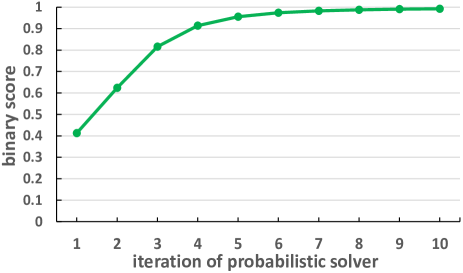
Figure 3: The illustration for convergence of the proposed probabilistic solver.

In experiments, we follow [22] to extract the visual features using the VGG16 backbone [47] as the raw keypoint features. The encoder transforms both the initial node features and edge features on AA-graph to the 128-dimension latent space for the graph matching tasks on the Pascal VOC [26] and SPair-71k [27] datasets. In other words, both $d_{V}$ and $d_{E}$ are set as 128. For the much easier Willow [16] dataset, the encoder transforms the AA-graph features to 32-dimension latent space (i.e., $d_{V}=d_{E}=32$) to alleviate the over-fitting during training. For gradient back propagation in model learning, the gradients of the solution would be very small when the solution is close to $\{0,1\}$ after many iterations of the probabilistic solver, making the model hard to be trained. Considering that, we adopt an early-stop strategy to avoid gradient vanishing, which is formulated at Lines 7 to 9 in Algorithm 1. Specifically, if the increment of the updated assignments is below a predefined threshold $\eta$, the updating of assignments and affinities will be stopped. Furthermore, we set the iteration of the convolution operation in the AA-prediction network as 5 to capture the structural representations from 5-order neighborhoods. In the probabilistic solver, we specify the stop threshold $\eta=0.00001$ and the iteration maximum $S=10$ throughout our experiments. During training, the positive label weight $w$ in Eq. 13 is fixed to 5 to balance the significance of positive labels and negative labels. Our model runs on a linux server with Intel(R) Xeon(R) CPU E5-2620 v4 (2.10GHz) and a TITAN XP GPU (12G).

TABLE I: Comparison of matching accuracy (%) on the Willow Object dataset. Bold numbers represent the best results.

Algorithm	Car	Duck	Face	Motorb.	Wineb.	AVG
GMN [17]	74.3	82.8	99.3	71.4	76.7	80.9
PCA [18]	84.0	93.5	100	76.7	96.9	90.2
IPCA [44]	90.2	84.9	100	77.7	95.2	89.6
LGM [19]	91.2	86.2	100	99.4	97.9	94.9
qc-DGM [20]	98.0	92.8	100	98.8	99.0	97.7
DGMC [23]	98.3	90.2	100	98.5	98.1	97.0
CIE [24]	82.2	81.2	100	90.0	97.6	90.2
BBGM [22]	96.9	89.0	100	99.2	98.8	96.8
NGM [45]	97.4	93.4	100	98.6	98.3	97.5
NGMv2 [45]	97.4	93.4	100	98.6	98.3	97.5
DPGM (ours)	99.5	96.8	100	100	93.0	97.9

TABLE II: Comparison of matching accuracy (%) on the Pascal VOC dataset. Bold numbers represent the best results.

Algo.	aero	bike	bird	boat	bot.	bus	car	cat	cha.	cow	tab.	dog	hor.	mbi.	per.	pla.	she.	sofa	tra.	tv	AVG
GMN [17]	31.9	47.2	51.9	40.8	68.7	72.2	53.6	52.8	34.6	48.6	72.3	47.7	54.8	51.0	38.6	75.1	49.5	45.0	83.0	86.3	55.3
PCA [18]	51.2	61.3	61.6	58.4	78.8	73.9	68.5	71.1	40.1	63.3	45.1	64.4	66.4	62.2	45.1	79.1	68.4	60.0	80.3	91.9	64.6
IPCA [44]	51.0	64.9	68.4	60.5	80.2	74.7	71.0	73.5	42.2	68.5	48.9	69.3	67.6	64.8	48.6	84.2	69.8	62.0	79.3	89.3	66.9
LGM [19]	46.9	58.0	63.6	69.9	87.8	79.8	71.8	60.3	44.8	64.3	79.4	57.5	64.4	57.6	52.4	96.1	62.9	65.8	94.4	92.0	68.5
qc-DGM [20]	49.6	64.6	67.1	62.4	82.1	79.9	74.8	73.5	43.0	68.4	66.5	67.2	71.4	70.1	48.6	92.4	69.2	70.9	90.9	92.0	70.3
DGMC [23]	50.4	67.6	70.7	70.5	87.2	85.2	82.5	74.3	46.2	69.4	69.9	73.9	73.8	65.4	51.6	98.0	73.2	69.6	94.3	89.6	73.2
CIE [24]	51.2	69.2	70.1	55.0	82.8	72.8	69.0	74.2	39.6	68.8	71.8	70.0	71.8	66.8	44.8	85.2	69.9	65.4	85.2	92.4	68.9
BBGM [22]	61.5	75.0	78.1	80.0	87.4	93.0	89.1	80.2	58.1	77.6	76.5	79.3	78.6	78.8	66.7	97.4	76.4	77.5	97.7	94.4	80.1
NGM [45]	50.1	63.5	57.9	53.4	79.8	77.1	73.6	68.2	41.1	66.4	40.8	60.3	61.9	63.5	45.6	77.1	69.3	65.5	79.2	88.2	64.1
NGMv2 [45]	61.8	71.2	77.6	78.8	87.3	93.6	87.7	79.8	55.4	77.8	89.5	78.8	80.1	79.2	62.6	97.7	77.7	75.7	96.7	93.2	80.1
DPGM (ours)	63.1	64.5	78.5	81.4	93.8	93.5	90.0	81.5	56.9	80.6	95.0	80.3	80.3	72.5	68.0	98.5	79.3	75.4	98.3	92.8	81.2

TABLE III: Comparison of matching accuracy (%) on the Pascal VOC dataset with filtered image pairs. Bold numbers represent the best results.

Algo.	aero	bike	bird	boat	car	cat	cha.	cow	dog	hor.	mbi.	per.	she.	sofa	AVG
GMN [17]	36.2	60.5	33.8	46.4	71.9	64.6	29.5	58.1	54.4	57.5	54.1	35.4	58.9	100.0	54.4
IPCA [44]	51.2	67.2	40.6	42.1	71.9	72.4	34.0	63.6	63.3	65.8	68.2	47.6	65.2	100.0	60.9
CIE [24]	45.7	62.4	40.0	40.7	66.3	74.1	31.4	64.5	65.4	68.1	55.6	44.9	63.9	80.0	57.4
BBGM [22]	57.0	72.6	50.0	60.7	88.6	79.7	44.8	75.8	76.9	76.5	71.5	64.6	71.2	100.0	70.7
NGMv2 [45]	54.9	73.0	49.3	50.0	86.3	79.7	49.0	76.5	74.2	74.3	73.6	61.5	72.9	100.0	69.7
DPGM (ours)	55.5	66.2	52.3	58.4	91.3	81.4	47.9	74.9	76.5	80.6	71.7	72.1	73.3	100.0	71.6

TABLE IV: Comparison of matching accuracy (%) on the SPair-71k dataset. Bold numbers represent the best results.

Algo.	aero	bike	bird	boat	bott.	bus	car	cat	chair	cow	dog	hor.	mbi.	per.	plant	she.	train	tv	AVG
DGMC [23]	54.8	44.8	80.3	70.9	65.5	90.1	78.5	66.7	66.4	73.2	66.2	66.5	65.7	59.1	98.7	68.5	84.9	98.0	72.2
BBGM [22]	66.9	57.7	85.8	78.5	66.9	95.4	86.1	74.6	68.3	78.9	73.0	67.5	79.3	73.0	99.1	74.8	95.0	98.6	78.9
DPGM (ours)	68.5	64.0	86.6	76.9	72.4	96.4	81.9	75.9	65.6	81.1	73.0	73.1	82.2	76.2	98.7	83.1	89.0	99.9	80.3

5.1 Willow Object dataset

The Willow Object dataset provided in [16] contains 5 categories, each of which is represented by at least 40 images with different instances. Each image in this dataset is annotated with 10 distinctive landmarks on the target object, which means there is no outlier keypoint between two images from the same category. Following the dataset split setting in [18, 19], we select 20 images from each category for training and keep the rest for testing. Note that any two images from the same class of the training set can form a training sample, and we thus obtain a total of 2,000 training samples. In testing, we randomly choose 1,000 pairs of images from the testing set of each category respectively.

The graph matching performances of the compared approaches are shown in Table I. This dataset is considered relatively easy due to the lack of variation in pose, scale and illumination, thus most of the compared methods achieve excellent matching results, especially on the Face category. By jointly learning pairwise affinities and initial node assignments, our method solves the quadratic assignment problem without relaxation on the constraints in a deep probabilistic scheme. As a result, our method achieves the best matching accuracy in all categories expect Winebottle, and surpasses all compared baselines in general.

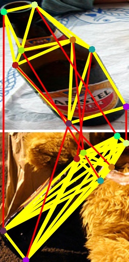
(a) GMN: 0/8

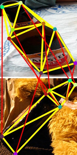
(b) PCA: 0/8

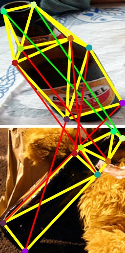
(c) IPCA: 2/8

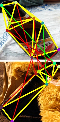
(d) CIE: 2/8

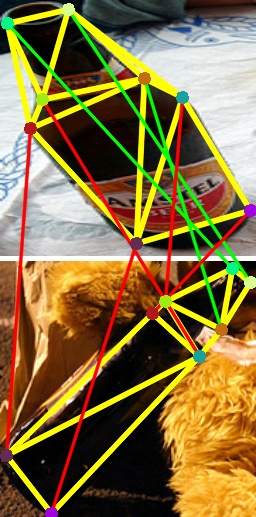
(e) DGMC: 3/8

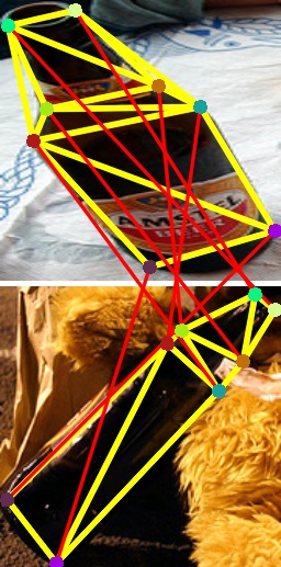
(f) LGM: 0/8

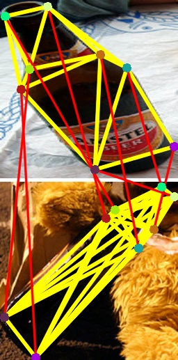
(g) NGM: 0/8

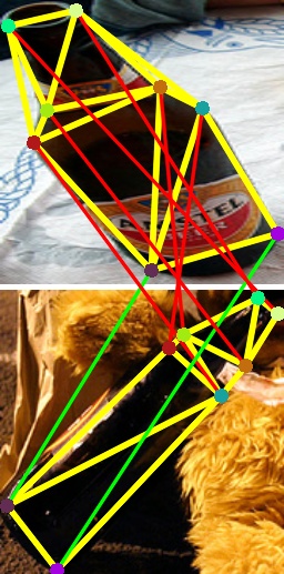
(h) NGMv2: 2/8

(i) BBGM: 2/8

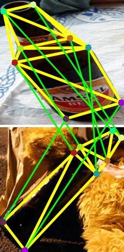
(j) DPGM(ours): 8/8

Figure 4: The representative examples of matching results solved by all compared methods on category bottle. The keypoints with same semantic annotations are marked in the same colors. The graph structures built in each image are represented as yellow lines. The incorrect and correct matches are represented as red lines and green lines across each pair of images, respectively.

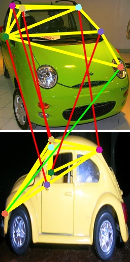
(a) GMN: 1/6

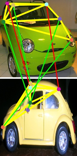
(b) PCA: 4/6

(c) IPCA: 2/6

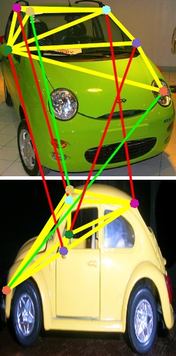
(d) CIE: 2/6

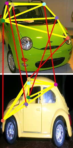
(e) DGMC: 0/6

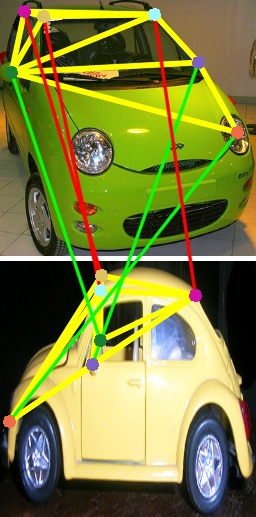
(f) LGM: 3/6

(g) NGM: 2/6

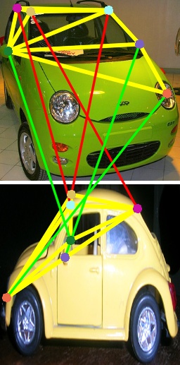
(h) NGMv2: 3/6

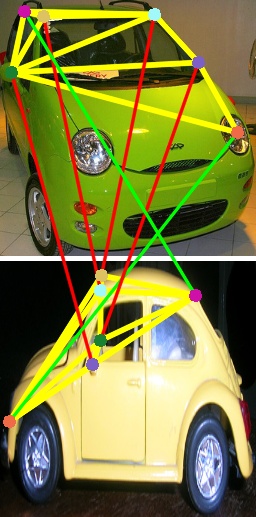
(i) BBGM: 2/6

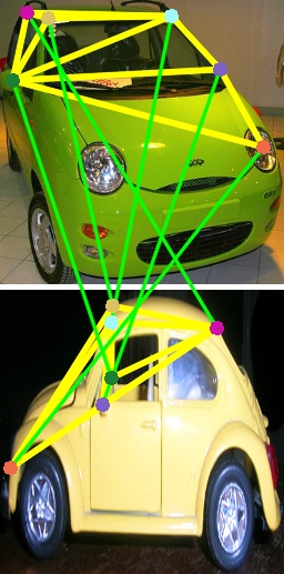
(j) DPGM(ours): 6/6

Figure 5: The representative examples of matching solutions solved by all compared methods on category car. The keypoints with same semantic annotations are marked in the same colors. The graph structures built in each image are represented as yellow lines. The incorrect and correct matches are represented as red lines and green lines across each pair of images, respectively.

5.2 Pascal VOC

Pascal VOC [26] with Berkeley annotations of keypoints [48] contains 20 classes of instances with labeled keypoint locations. This dataset is considered more challenging than the Willow dataset for that instances may vary in its scale, pose, illumination and the number of inlier keypoints. Following previous arts [18, 19], we split the dataset into two groups, i.e., 7,020 annotated images for training and 1,682 images for testing. In particular, we randomly select 1,000 pairs of images from the testing set of each category for testing.

The comparison results on Pascal VOC [26] have been illustrated in Table II. Most of the previous methods [18, 44, 19, 20, 23, 24] that solve the graph matching problem in a relaxed form fail to provide satisfying matching results. After embedding a stronger combinatorial solver, BBGM [22], NGMv2 [45] and our DPGM gain remarkable improvement in matching accuracy. In particular, our method achieves the best results on 14 categories and rises the average matching accuracy to $81.2\%$, surpassing the strongest competitors BBGM [22] and NGMv2 [45] by $1.1\%$. Some representative matching results of compared methods on categories bottle and car have been illustrated in Figs. 4 and 5, respectively, both of which refer to the visual matching under heavy view changes. As illustrated in Figs. 4 and 5, the previous deep learning methods, even those combined with combinatorial solvers, fail to obtain satisfied matching results. While with the proposed probabilistic solvers for searching the optimal solution from predicted assignments, our model DPGM achieves the best matching results where all the correct matches have been found.

Table II illustrates the comparison of matching results on Pascal VOC [26] where each image pair may not contain the same keypoints, and all the compared methods only match an intersection of the two set of keypoints. However, this will lead to a problem that in many cases there may be only two 2 or 3 keypoints left. In such cases, what may contribute to the results is better visual feature, and the graph matching algorithm can not do much to improve the performance of the algorithm. Therefore, we perform an additional experiments on the Pascal VOC [26] dataset with filtered image pairs that contain at least 10 keypoints, for better validation of the contribution of graph matching algorithms. The comparison is reported in Table III where only 14 categories of image pairs with at least 10 keypoints are kept. As illustrated in Table III, all algorithms achieve relatively lower matching accuracies in comparison with that in the original Pascal VOC dataset (Table 2). This demonstrates that finding optimal matching between relatively large graphs is more difficult than that on small ones. While consistent with the results in Table II, BBGM [22] and NGMv2 [45], which embed combinatorial solvers into deep graph matching framework, achieve relatively higher average matching accuracy than other baselines. This again demonstrates that the combination of combinatorial solvers and deep affinity learning framework is more suitable for graph matching tasks. Furthermore, with the proposed probabilistic solver, our algorithm achieves comparable or even best matching accuracy on most categories in comparison with previous state-of-the-art baselines, and rises the average matching accuracy to 71.6%, surpassing the strong competitors BBGM [22] and NGMv2 [45] by 0.9% and 1.9%, respectively, which validates the effectiveness of the proposed deep probabilistic solver.

TABLE V: Comparison of inferring time (ms) on Willow and Pascal VOC.

Dataset	GMN	LGM	NGM	NGMv2	PCA	IPCA	DGMC	CIE	BBGM	DPGM (ours)
Willow [16]	28	42	14	15	29	35	3	28	13	10
Pascal VOC [26]	27	33	12	13	26	30	4	26	11	30

5.3 SPair-71k

The SPair-71k [27] is another large-scale benchmark dataset including a total of 70,958 pairs of images from PASCAL 3D+ [49] and Pascal VOC 2012 [50], which is very well organized with rich annotations for learning. Compared with Pascal VOC [26], the pair annotations in this dataset have larger variations in view-point, scale, truncation and occlusion, thus reflecting the more generalized visual correspondence problem in real-world scenarios. In addition, it removes the ambiguous and poorly annotated categories, i.e., sofa and dining table, from the Pascal VOC dataset [26].

The matching accuracy on SPair-71k [27] are reported in Table IV, where two state-of-the-art algorithms DGMC [23] and BBGM [22] are taken as the baselines in comparison with our method. Compared with DGMC [23], the strongest competitor BBGM [22] that employs a heavily optimized solver for graph matching achieves 6.7% improvements on average matching accuracy, which demonstrates the effectiveness of the combination of deep framework for affinity learning and combinatorial solver. Furthermore, with the proposed probabilistic solver, our model DPGM achieves the best performance on most categories and reaches the best average matching accuracy of $80.3\%$, surpassing the DGMC [23] and BBGM [22] by $8.1\%$ and $1.4\%$ respectively, which reveals that our method can be well generalized to more difficult graph matching problems in real-world scenarios.

5.4 Running Time

In addition to matching accuracy, computational efficiency is another important evaluation metric for graph matching methods. In this subsection, we report the inferring time of our algorithm in comparison with several deep-learning algorithms on the Pascal VOC [26] and Willow [16] datasets. The comparisons for inferring time have been illustrated in Table V. It is observed that, our algorithm achieves the efficiency that is similar to or higher than GMN [17], LGM [19], NGM [45] and NGMv2 [45] that are also based on Lawler’ QAP formulation. On the other hand, all of them are in general comparable in computational efficiency with PCA [18], IPCA [44] and CIE [18], which have relaxed the quadratic constraints. As the latent dimensions of the proposed model on Willow [16] is relatively lower than that on Pascal VOC [26], our model is more efficient for dealing with the visual matching tasks on Willow [16] dataset. Specially, DGMC [23] is the most efficient one because the node features are complied in advance and the feature extraction module is removed from the code provided by the authors.

5.5 Ablation Studies

TABLE VI: Ablation studies on the Pascal VOC dataset. Bold numbers represent the best results.

Abl.	aero	bike	bird	boat	bott.	bus	car	cat	chair	cow	tab.	dog	hor.	mbi.	per.	plant	she.	sofa	train	tv	AVG
WPS	56.4	65.8	74.7	78.0	88.2	92.5	85.6	77.6	54.9	73.9	83.5	74.8	75.0	71.5	61.7	95.7	75.5	74.4	96.6	92.4	77.4
TIA	56.7	69.4	75.4	74.8	91.5	87.4	87.0	76.4	52.2	76.2	80.1	77.3	76.5	71.9	60.4	97.5	75.4	67.4	96.7	87.7	76.9
DPGM	63.1	64.5	78.5	81.4	93.8	93.5	90.0	81.5	56.9	80.6	95.0	80.3	80.3	72.5	68.0	98.5	79.3	75.4	98.3	92.8	81.2

TABLE VII: Ablation studies on the SPair-71k dataset. Bold numbers represent the best results.

Abl.	aero	bike	bird	boat	bott.	bus	car	cat	chair	cow	dog	hor.	mbi.	per.	plant	she.	train	tv	AVG
WPS	65.3	56.1	84.4	75.0	72.7	96.9	85.6	74.0	64.0	81.5	70.4	68.7	72.8	72.7	99.0	78.9	93.3	99.8	78.4
TIA	68.2	52.1	84.3	73.9	70.8	95.8	82.8	76.2	60.0	78.4	71.2	67.0	69.5	72.4	96.6	78.5	92.1	99.7	77.2
DPGM	68.5	64.0	86.6	76.9	72.4	96.4	81.9	75.9	65.6	81.1	73.0	73.1	82.2	76.2	98.7	83.1	89.0	99.9	80.3

TABLE VIII: Ablation studies on the Willow Object dataset. Bold numbers represent the best results.

Ablation	Car	Duck	Face	Motorb.	Wineb.	AVG
WPS	91.8	85.4	100	98.3	97.1	95.4
TIA	96.7	86.3	100	98.2	99.0	96.0
DPGM	99.5	96.8	100	100	93.0	97.9

5.5.1 Contributions of learnt assignments and affinities

For illustration of the contributions of different modules in our framework, we provide various ablation studies and report results of two downgraded versions of our algorithm, named TIA and WPS, in Tables VI, VII, VIII.

Trivial initialization of assignments (TIA): we exclude the estimated assignments from the output of the AA-predictor, and initialize trivial assignments as the input of the probabilistic solver.

Without probabilistic solver (WPS): the differentiable probabilistic solver is removed from the network, and the output assignments of the AA-decoder are directly taken as the final solutions.

As shown in Tables VI, VII, VIII, both the downgraded versions of our model obtain inferior performance to the full version on all the three benchmarks. Especially for Pascal VOC [26], the full version of our model outperforms TIA and WPS by 4.3% and 3.8% on the average matching accuracy, respectively. These studies show that both the components make contributions to the excellent performance of the proposed DPGM algorithm.

Furthermore, we also explore the studies that combine the learnt affinities and other traditional learning-free solvers on Pascal VOC [26]. Specifically, we take the affinities learnt by our AA-prediction network as input, and adopt several state-of-the-art traditional learning-free solvers, including RRWM [5], PSM [7] and IPFP [51], to search the optimal solutions. The comparisons on Pascal VOC [26] are reported in Table IX, where RRWM-H and RRWM-L denote the results of using the handcrafted affinities and the learned ones, respectively. Same notations are used for PSM [7] and IPFP [51]. The results of using the handcrafted affinities are cited from LGM [19]. Obviously, replacing the handcrafted affinities with the learned ones can significantly improve the matching accuracies in most categories, and rise the average matching accuracies by 35.6%, 37.3% and 39.2% for RRWM [5], PSM [7] and IPFP [51], respectively. It clearly demonstrates the effectiveness of the learned affinities by our framework for graph matching. On the other hand, even though the learnt affinities are combined, these traditional solvers are still inferior to our framework by a certain gaps. It indicates that the learnt affinities are more suitable for end-to-end learnable framework than the transitional learning-free solvers.

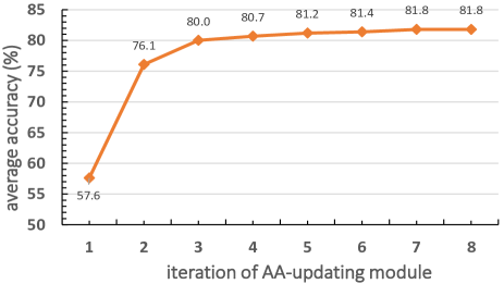
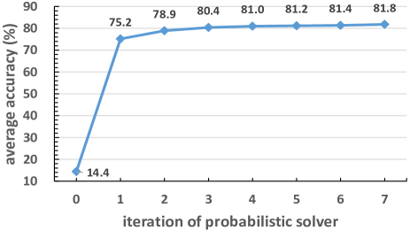
Figure 6: Results in the ablation experiments on the number of iterations for (a) the AA-updating module and (b) the probabilistic solver.

TABLE IX: Comparison of matching accuracy (%) on the Pascal VOC dataset under the combination of learnt affinities and traditional learning-free solvers. Bold numbers represent the best results.

Algo.	aero	bike	bird	boat	bot.	bus	car	cat	cha.	cow	tab.	dog	hor.	mbi.	per.	pla.	she.	sofa	tra.	tv	AVG
RRWM-H	30.9	40.0	46.4	54.1	52.3	35.6	47.4	37.3	36.3	34.1	28.8	35.0	39.1	36.2	39.5	67.8	38.6	49.4	70.5	41.3	43.0
RRWM-L	61.5	61.0	76.8	79.8	93.1	91.4	88.5	78.2	54.2	76.8	98.2	75.5	76.0	69.5	65.5	98.1	75.8	68.9	88.6	93.6	78.6
PSM-H	32.6	37.5	49.9	53.2	47.8	34.6	50.1	35.5	37.2	36.3	23.1	32.7	42.4	37.1	38.5	62.3	41.7	54.3	72.6	40.8	43.1
PSM-L	62.4	64.3	78.0	81.3	93.2	93.0	89.9	81.3	55.6	79.9	100.0	78.0	80.0	72.2	66.8	98.3	77.2	73.2	90.6	93.9	80.4
IPFP-H	25.1	26.4	41.4	50.3	43.0	32.9	37.3	32.5	33.6	28.2	26.9	26.1	29.9	32.0	28.8	62.9	28.2	45.0	69.3	33.8	36.6
IPFP-L	59.5	59.1	74.2	78.1	91.4	87.7	85.7	76.4	52.3	73.8	84.7	73.8	73.9	66.7	62.8	97.8	73.9	67.6	84.1	93.6	75.8
DPGM	63.1	64.5	78.5	81.4	93.8	93.5	90.0	81.5	56.9	80.6	95.0	80.3	80.3	72.5	68.0	98.5	79.3	75.4	98.3	92.8	81.2

5.5.2 Iteration of AA-updating module

In the AA-predictor, the iteration of AA-updating module determines the receptive field of aggregated information from neighbors, which has direct influence to the final matching performance. Here, we vary the AA-updating iteration from 1 to 8 to explore its influence to the average matching accuracy. As illustrated in Fig. 6, the average matching accuracy is only 57.6% when only single iteration of AA-updating is performed. While the performance of our model can be significantly improved by setting the iteration of AA-updating from 2 to 5. However, there is no evident improvement when the iteration of AA-updating module is set as a value greater than 5, which demonstrates only 5 iterations of AA-updating module is sufficient to capture the structural representations of AA-graph. This in turn explain why we set the convolution iteration in AA-predictor as 5.

5.5.3 Iteration of probabilistic solver

Given the predicted assignments and affinities by AA-predictor, the proposed probabilistic solver refines them iteratively to search the optimal solution. To explore the influence of iteration of probabilistic solver to the model performance, we vary the refinement iteration for assignments from 0 to 7. As illustrated in Fig. 6, without refinement for assignments, i.e., setting the refinement iteration as 0, the average matching accuracy is only 14.4%. With a single iteration of refinement for assignments, our model rises the matching accuracy to 75.2%, which surpasses most of the state-of-the-art baselines. When setting the iteration of probabilistic solver as a value greater than 4, the average matching accuracy is stable around 81.0%. The illustration of results in Fig. 6 and the convergence showed in Fig 3 reveal that our model needs not many refinement iteration to search the optimal solutions, which guarantees the efficiency of the proposed model.

6 Conclusion

In this paper, we propose a novel deep learning algorithm, named DPGM, for graph matching. In DPGM, an affinity-assignment prediction network is developed to learn the pairwise affinities and at the same time estimate the initial node assignments, and a differentiable solver is embedded to better optimize the QAP in a probabilistic perspective without compromise on the matching constraints. Experimental results reveal that DPGM achieves state-of-the-art matching performance on various real-world image datasets.

He Liu received the B. S. degree in compute science from Hebei University of Technology, Tianjin, China. He is currently pursuing the Ph. D degree in the School of Computer and Information Technology, Beijing Jiaotong University, Beijing, China. His research concentrates on machine learning and graph matching.

Tao Wang received the PhD degree from the School of Computer and Information Technology, Beijing Jiaotong University, Beijing, China, in 2013. He was a visiting professor with the Department of Computer and Information Sciences, Temple University, from 2014 to 2015. He is currently an associate professor with the School of Computer and Information Technology, Beijing Jiaotong University. His research interests include graph matching theory with application to image analysis and retrieval.

Yidong Li was born in 1982, native to Shanxi, associate professor and Ph.D. supervisor. In 2003, he graduated from the Department of information and communication engineering of Beijing Jiaotong University. He received master and Ph. D. degree from the department of computer science of the University of Adelaide in Australia in 2006 and 2011 respectively. Dr. Yi is the vice dean of the school of computer and information technology, Beijing Jiaotong University, executive director of the SAP University Competence Center (China).

Congyan Lang received her Ph.D. degree from the School of Computer and Information Technology, Beijing Jiaotong University, Beijing, China, in 2006. She was a Visiting Professor with the Department of Electrical and Computer Engineering, National University of Singapore, Singapore, from 2010 to 2011. From 2014 to 2015, she visited the Department of Computer Science, University of Rochester, Rochester, NY, USA, as a Visiting Professor. She is currently a Professor with the School of Computer and Information Technology, Beijing Jiaotong University. Her research areas include computer vision, machine learning, object recognition and segmentation.

Songhe Feng received the Ph.D. degree from the School of Computer and Information Technology, Beijing Jiaotong University, Beijing, China, in 2009. He was a Visiting Scholar with the Department of Computer Science and Engineering, Michigan State University, USA, from 2013 to 2014. He is currently a Professor with the School of Computer and Information Technology, Beijing Jiaotong University. His research interests include computer vision and machine learning.

Haibin Ling received Ph.D. degree from University of Maryland in 2006. From 2007-2008, he worked for Siemens Corporate Research as a research scientist; and from 2008 to 2019, he was a faculty member of the Department of Computer Sciences for Temple University. In fall 2019, he joined the Department of Computer Science of Stony Brook University, where he is now a SUNY Empire Innovation Professor. His research interests include computer vision, augmented reality, medical image analysis, visual privacy protection, and human computer interaction.

References

- [1] Y. Song, C. Li, L. Wang, P. M. Hall, and P. Shen, “Robust visual tracking using structural region hierarchy and graph matching,” Neurocomputing, vol. 89, pp. 12–20, 2012.
- [2] T. Wang and H. Ling, “Gracker: A graph-based planar object tracker,” IEEE Trans. Pattern Anal. Mach. Intell., vol. 40, no. 6, pp. 1494–1501, 2018.
- [3] M. Ye, A. J. Ma, L. Zheng, J. Li, and P. C. Yuen, “Dynamic label graph matching for unsupervised video re-identification,” in Int. Conf. Comput. Vis., 2017, pp. 5152–5160.
- [4] C. Leng, W. Xu, I. Cheng, and A. Basu, “Graph matching based on stochastic perturbation,” IEEE Trans. Image Process., vol. 24, no. 12, pp. 4862–4875, 2015.
- [5] M. Cho, J. Lee, and K. M. Lee, “Reweighted random walks for graph matching,” in Eur. Conf. Comput. Vis., vol. 6315, 2010, pp. 492–505.
- [6] T. Cour, P. Srinivasan, and J. Shi, “Balanced graph matching,” in Adv. Neural Inform. Process. Syst., 2006, pp. 313–320.
- [7] A. Egozi, Y. Keller, and H. Guterman, “A probabilistic approach to spectral graph matching,” IEEE Trans. Pattern Anal. Mach. Intell., vol. 35, no. 1, pp. 18–27, 2013.
- [8] S. Gold and A. Rangarajan, “A graduated assignment algorithm for graph matching,” IEEE Trans. Pattern Anal. Mach. Intell., vol. 18, no. 4, pp. 377–388, 1996.
- [9] M. Leordeanu and M. Hebert, “A spectral technique for correspondence problems using pairwise constraints,” in Int. Conf. Comput. Vis., 2005, pp. 1482–1489.
- [10] Z. Liu and H. Qiao, “GNCCP - graduated nonconvexityand concavity procedure,” IEEE Trans. Pattern Anal. Mach. Intell., vol. 36, no. 6, pp. 1258–1267, 2014.
- [11] T. Wang, H. Ling, C. Lang, and S. Feng, “Graph matching with adaptive and branching path following,” IEEE Trans. Pattern Anal. Mach. Intell., vol. 40, no. 12, pp. 2853–2867, 2018.
- [12] M. Zaslavskiy, F. R. Bach, and J. Vert, “A path following algorithm for the graph matching problem,” IEEE Trans. Pattern Anal. Mach. Intell., vol. 31, no. 12, pp. 2227–2242, 2009.
- [13] R. Zass and A. Shashua, “Probabilistic graph and hypergraph matching,” in IEEE Conf. Comput. Vis. Pattern Recog., 2008, pp. 1–8.
- [14] F. Zhou and F. D. la Torre, “Factorized graph matching,” IEEE Trans. Pattern Anal. Mach. Intell., vol. 38, no. 9, pp. 1774–1789, 2016.
- [15] T. S. Caetano, J. J. McAuley, L. Cheng, Q. V. Le, and A. J. Smola, “Learning graph matching,” IEEE Trans. Pattern Anal. Mach. Intell., vol. 31, no. 6, pp. 1048–1058, 2009.
- [16] M. Cho, K. Alahari, and J. Ponce, “Learning graphs to match,” in Int. Conf. Comput. Vis., 2013, pp. 25–32.
- [17] A. Zanfir and C. Sminchisescu, “Deep learning of graph matching,” in IEEE Conf. Comput. Vis. Pattern Recog., 2018, pp. 2684–2693.
- [18] R. Wang, J. Yan, and X. Yang, “Learning combinatorial embedding networks for deep graph matching,” in Int. Conf. Comput. Vis., 2019, pp. 3056–3065.
- [19] T. Wang, H. Liu, Y. Li, Y. Jin, X. Hou, and H. Ling, “Learning combinatorial solver for graph matching,” in IEEE Conf. Comput. Vis. Pattern Recog., 2020, pp. 7565–7574.
- [20] Q. Gao, F. Wang, N. Xue, J.-G. Yu, and G.-S. Xia, “Deep graph matching under quadratic constraint,” in IEEE Conf. Comput. Vis. Pattern Recog., 2021, pp. 5069–5078.
- [21] P. Sarlin, D. DeTone, T. Malisiewicz, and A. Rabinovich, “Superglue: Learning feature matching with graph neural networks,” in IEEE Conf. Comput. Vis. Pattern Recog., 2020, pp. 4937–4946.
- [22] M. Rolínek, P. Swoboda, D. Zietlow, A. Paulus, V. Musil, and G. Martius, “Deep graph matching via blackbox differentiation of combinatorial solvers,” in Eur. Conf. Comput. Vis., vol. 12373, 2020, pp. 407–424.
- [23] M. Fey, J. E. Lenssen, C. Morris, J. Masci, and N. M. Kriege, “Deep graph matching consensus,” in Int. Conf. Learn. Represent., 2020.
- [24] T. Yu, R. Wang, J. Yan, and B. Li, “Learning deep graph matching with channel-independent embedding and hungarian attention,” in Int. Conf. Learn. Represent., 2020.
- [25] G. Mena, D. Belanger, G. Munoz, and J. Snoek, “Sinkhorn networks: Using optimal transport techniques to learn permutations,” in NIPS Workshop Optim. Transp. Mach. Learn., 2017, pp. 1–10.
- [26] M. Everingham, L. V. Gool, C. K. I. Williams, J. M. Winn, and A. Zisserman, “The pascal visual object classes (VOC) challenge,” Int. J. Comput. Vis., vol. 88, no. 2, pp. 303–338, 2010.
- [27] J. Min, J. Lee, J. Ponce, and M. Cho, “Spair-71k: A large-scale benchmark for semantic correspondence,” CoRR, vol. abs/1908.10543, 2019. [Online]. Available: http://arxiv.org/abs/1908.10543
- [28] D. Conte, P. Foggia, C. Sansone, and M. Vento, “Thirty years of graph matching in pattern recognition,” Int. J. Pattern Recognit. Artif. Intell, vol. 18, no. 3, pp. 265–298, 2004.
- [29] P. Foggia, G. Percannella, and M. Vento, “Graph matching and learning in pattern recognition in the last 10 years,” Int. J. Pattern Recognit. Artif. Intell, vol. 28, no. 1, pp. 1–40, 2014.
- [30] J. Yan, X. Yin, W. Lin, C. Deng, H. Zha, and X. Yang, “A short survey of recent advances in graph matching,” in Int. Conf. Multimed. Retr., 2016, pp. 167–174.
- [31] M. Leordeanu, R. Sukthankar, and M. Hebert, “Unsupervised learning for graph matching,” Int. J. Comput. Vis., vol. 96, no. 1, pp. 28–45, 2012.
- [32] M. Leordeanu, A. Zanfir, and C. Sminchisescu, “Semi-supervised learning and optimization for hypergraph matching,” in Int. Conf. Comput. Vis., 2011, pp. 2274–2281.
- [33] M. Leordeanu and M. Hebert, “Smoothing-based optimization,” in IEEE Conf. Comput. Vis. Pattern Recog., 2008.
- [34] L. Shi, Y. Zhang, J. Cheng, and H. Lu, “Skeleton-based action recognition with multi-stream adaptive graph convolutional networks,” IEEE Trans. Image Process., vol. 29, pp. 9532–9545, 2020.
- [35] X. Hao, J. Li, Y. Guo, T. Jiang, and M. Yu, “Hypergraph neural network for skeleton-based action recognition,” IEEE Trans. Image Process., vol. 30, pp. 2263–2275, 2021.
- [36] A. Nowak, S. Villar, A. S. Bandeira, and J. Bruna, “Revised note on learning quadratic assignment with graph neural networks,” in IEEE Data Sci. Workshop, 2018, pp. 229–233.
- [37] T. N. Kipf and M. Welling, “Semi-supervised classification with graph convolutional networks,” in Int. Conf. Learn. Represent., 2017.
- [38] P. Swoboda, C. Rother, H. A. Alhaija, D. Kainmüller, and B. Savchynskyy, “A study of lagrangean decompositions and dual ascent solvers for graph matching,” in IEEE Conf. Comput. Vis. Pattern Recog., 2017, pp. 7062–7071.
- [39] E. M. Loiola, N. M. M. de Abreu, P. O. B. Netto, P. Hahn, and T. M. Querido, “A survey for the quadratic assignment problem,” Eur. J. Oper. Res., vol. 176, no. 2, pp. 657–690, 2007.
- [40] M. Frank and P. Wolfe, “An algorithm for quadratic programming,” Nav. Res. Logist. Q., vol. 3, pp. 95–100, 1956.
- [41] R. Sinkhorn, “A relationship between arbitrary positive matrices and doubly stochastic matrices,” Ann. Math. Stat, vol. 35, no. 2, pp. 876–879, 1964.
- [42] M. Fey, J. E. Lenssen, F. Weichert, and H. Müller, “Splinecnn: Fast geometric deep learning with continuous b-spline kernels,” in IEEE Conf. Comput. Vis. Pattern Recog., 2018, pp. 869–877.
- [43] Y. LeCun, Y. Bengio et al., “Convolutional networks for images, speech, and time series,” Handb. Brain Theory Neural Netw., vol. 3361, no. 10, p. 1995, 1995.
- [44] R. Wang, J. Yan, and X. Yang, “Combinatorial learning of robust deep graph matching: an embedding based approach,” IEEE Trans. Pattern Anal. Mach. Intell., 2020.
- [45] Wang, Runzhong and Yan, Junchi and Yang, Xiaokang, “Neural graph matching network: Learning lawler’ s quadratic assignment problem with extension to hypergraph and multiple-graph matching,” IEEE Trans. Pattern Anal. Mach. Intell., 2021.
- [46] T. Yu, R. Wang, J. Yan, and B. Li, “Deep latent graph matching,” in Int. Conf. Mach. Learn., vol. 139, 2021, pp. 12 187–12 197.
- [47] K. Simonyan and A. Zisserman, “Very deep convolutional networks for large-scale image recognition,” in Int. Conf. Learn. Represent., Y. Bengio and Y. LeCun, Eds., 2015.
- [48] L. D. Bourdev and J. Malik, “Poselets: Body part detectors trained using 3d human pose annotations,” in Int. Conf. Comput. Vis., 2009, pp. 1365–1372.
- [49] Y. Xiang, R. Mottaghi, and S. Savarese, “Beyond PASCAL: A benchmark for 3d object detection in the wild,” in IEEE Winter Conf. Appl. Comput. Vis., 2014, pp. 75–82.
- [50] M. Everingham, S. M. A. Eslami, L. V. Gool, C. K. I. Williams, J. M. Winn, and A. Zisserman, “The pascal visual object classes challenge: A retrospective,” Int. J. Comput. Vis., vol. 111, no. 1, pp. 98–136, 2015.
- [51] M. Leordeanu, M. Hebert, and R. Sukthankar, “An integer projected fixed point method for graph matching and MAP inference,” in Adv. Neural Inform. Process. Syst., 2009, pp. 1114–1122.