FedBalancer: Data and Pace Control for Efficient Federated Learning on Heterogeneous Clients

Abstract.

Federated Learning (FL) trains a machine learning model on distributed clients without exposing individual data. Unlike centralized training that is usually based on carefully-organized data, FL deals with on-device data that are often unfiltered and imbalanced. As a result, conventional FL training protocol that treats all data equally leads to a waste of local computational resources and slows down the global learning process. To this end, we propose , a systematic FL framework that actively selects clients’ training samples. Our sample selection strategy prioritizes more “informative” data while respecting privacy and computational capabilities of clients. To better utilize the sample selection to speed up global training, we further introduce an adaptive deadline control scheme that predicts the optimal deadline for each round with varying client training data. Compared with existing FL algorithms with deadline configuration methods, our evaluation on five datasets from three different domains shows that improves the time-to-accuracy performance by 1.20$\sim$4.48$\times$ while improving the model accuracy by 1.1$\sim$5.0%. We also show that is readily applicable to other FL approaches by demonstrating that improves the convergence speed and accuracy when operating jointly with three different FL algorithms.

1. Introduction

Federated learning (FL) is a machine learning paradigm that performs decentralized training of models on mobile devices (e.g., smartphones) with locally stored data (McMahan et al., 2017). FL trains on a large corpus of private user data without collecting them, with only the model weight updates communicated externally from the user’s device (Bonawitz et al., 2019). With FL, researchers have proposed to improve AI in diverse domains: human mobility prediction (Feng et al., 2020), RF localization (Ciftler et al., 2020), traffic sign classification (Albaseer et al., 2020), tumour detection (Li et al., 2019a; Jiménez-Sánchez et al., 2021), and Clinical Decision Support (CDS) model for COVID-19 (Dayan et al., 2021). FL also has product deployments as large companies such as Google or Taobao deploy language processing and item recommendation tasks across millions of real-world devices (Niu et al., 2020; Yang et al., 2018).

One of the key objectives in FL is to optimize time-to-accuracy performance, which is a wall clock time for a model to achieve the target accuracy (Lai et al., 2021). Achieving high time-to-accuracy performance is important as FL consumes significant computation and network resources on edge-user devices (Dinh et al., 2021). For model developers who prototype a mobile AI with FL without a proxy dataset, achieving faster convergence on thousands to millions of devices is desired to efficiently test multiple model architectures and hyperparameters (Kairouz et al., 2019). Service providers who frequently update a model with continual learning with FL require to minimize the user overhead with better time-to-accuracy performance (Le et al., 2021).

In realistic FL scenarios, however, heterogeneous data being distributed over isolated users becomes the main challenge in achieving high time-to-accuracy performance (Zhao et al., 2018; Li et al., 2021a). While data engineering techniques such as importance sampling (Katharopoulos and Fleuret, 2018; Alain et al., 2015; Loshchilov and Hutter, 2015; Schaul et al., 2016) are widely adopted in centralized learning to optimize the training process, applying them in FL is infeasible as it requires private user data sharing. For this reason, previous FL algorithms (McMahan et al., 2017; Li et al., 2020a; Lai et al., 2021) mostly treat every client data equally, which could result in a waste of computational resources and slow convergence. We conducted a preliminary study to examine this phenomenon and found that the ratio of informative samples is reduced from 93.2% to 20% as the FL progresses. This could further exacerbate with heterogeneous hardware of FL clients, as low-end devices might fail to send model updates while training a large portion of unimportant samples.

To address this problem, we propose , a systematic FL framework with sample selection. The sample selection of prioritizes more “informative” samples of clients to efficiently utilize their computational effort. This allows low-end devices to contribute to the global training within the round deadline by focusing on smaller but more important training samples. To achieve high time-to-accuracy performance, the sample selection is designed to operate without additional forward or backward pass for sample utility measurement at FL rounds. Lastly, can coexist and collaborate with orthogonal FL approaches to further improve performance.

To realize , we addressed the following challenges: (1) Simply reducing the training data of a client with random sampling could lead to lower model accuracy as the statistical utility of the training data would decrease. As such, selects samples based on their statistical utility measurement. (2) Collecting sample-level statistical utility for sample selection might break the privacy guarantee of FL. To address this problem, we propose client-server coordination to maintain loss threshold, which allows clients to effectively select important samples while only exposing differentially-private statistics of their data. (3) The sample selection itself might not directly lead to time-to-accuracy performance improvement when the FL round deadline remains fixed. To formulate the benefit of selecting different deadlines, we propose a metric deadline efficiency (DDL-E) that calculates the number of round-completed clients per time. This allows to predict the optimal deadline with varying client training data.

We implemented and conducted experiments on five datasets from three domains that contain real-world user data. Compared with existing FL aggregation algorithms with deadline configuration methods, improves the time-to-accuracy performance by 1.20$\sim$4.48$\times$. achieves this improvement without sacrificing model accuracy; in fact, it improves the accuracy by 1.1%$\sim$5.0%. In addition, we implement on top of three orthogonal FL algorithms to demonstrate that is easily applicable to other FL approaches and improves their time-to-accuracy performance.

We summarize our contributions as follows:

• We propose a systematic framework for FL with sample selection, which actively selects high utility samples at each round without collecting privacy-invasive sample-level information from clients.

• We propose a deadline control strategy for each round of FL based on the newly defined metric deadline efficiency, which optimizes the time-to-accuracy performance along with our sample selection.

• We implement jointly with existing FL algorithms, showing improvement in both time-to-accuracy and model accuracy.

2. Background and Motivation

2.1. Federated Learning

Federated Learning (FL) operates across multiple mobile devices to globally train a model from the distributed client data. FedAvg (McMahan et al., 2017), the most commonly used FL approach (Jiang et al., 2020), operates as follows: (i) Suppose there are $N$ clients in an FL system. For each round of FL, the server randomly selects $K$ clients ($K<<N$) who participate in model training. (ii) At the R-th round, the server transmits the current model weights $\displaystyle{w}_{R}$ to the selected clients. (iii) Each client then performs model training for $E$ epochs with their local data and generates $\displaystyle{w}^{k}_{R+1}$, where $k$ denotes the client index. (iv) Clients upload the updated model parameters to the server, and (v) the server aggregates different clients’ updates and generate the updated model as ${w}_{R+1}\leftarrow\sum^{K}_{k=1}{\frac{n_{k}}{n}}{{w}^{k}_{R+1}}$, where $n_{k}$ indicates the number of data points of client $k$ and $n$ the number of all data points.

A key objective in FL is to optimize time-to-accuracy performance. FL tasks typically require hundreds to thousands of rounds to converge (Caldas et al., 2018; Lai et al., 2021), and clients participating at a round undergo substantial computational and network overhead (Dinh et al., 2021). Deploying FL across thousands to millions of devices should be done efficiently, quickly reaching the model convergence while not sacrificing the model accuracy. This becomes more important when FL has to be done multiple times, as often the case when model developers prototype a new model with FL without a proxy dataset or periodically update a deployed model to new domain via continual learning or online learning with FL.

However, the heterogeneities of the real-world mobile clients make it challenging to achieve good time-to-accuracy performance.
Data heterogeneity: The client-generated training data are imbalanced and not independent and identically distributed (non-IID) due to each user’s different mobile device usage or physical and mental characteristics (McMahan et al., 2017; Wu et al., 2020). While the training data in centralized learning could be filtered and organized with data engineering techniques (Katharopoulos and Fleuret, 2018; Alain et al., 2015; Loshchilov and Hutter, 2015; Schaul et al., 2016) to address data heterogeneity, applying the same solution is infeasible in FL as it is dealing with distributed private data on clients. Such data heterogeneity of FL clients results in slow convergence and suboptimal performance (Li et al., 2020a; Zhao et al., 2018; Li et al., 2021a).
Hardware heterogeneity: The client devices have distinct computational capabilities and network connectivity, resulting in up to 12$\times$ more round completion time between different clients (Li et al., 2019b). Thus, waiting for every client to complete its task at a round might significantly delay the training process. A common practice for such an issue is to set a deadline for a round duration and drop clients that fail to send the model updates before the deadline (Nishio and Yonetani, 2019; Abdelmoniem et al., 2021). However, this results in less contribution from clients with low-end devices, which could result in delayed convergence or biased model training (Yang et al., 2021; Li et al., 2020a).

2.2. Motivational Study

To address the heterogeneity problems, various approaches have been proposed. Researchers proposed FL algorithms that allow clients to train different numbers of local epochs (Li et al., 2020a) or different subsets of model weights (Diao et al., 2021; Horváth et al., 2021) based on clients’ hardware capabilities. Model personalization has also been proposed to tackle data heterogeneity (Pillutla et al., 2018; Ouyang et al., 2021; Fallah et al., 2020; Tu et al., 2021; Li et al., 2021c, b; Liu et al., 2020; Liu et al., 2021). In addition, client selection strategies for FL training have been proposed to optimize the convergence speed on heterogeneous clients (Lai et al., 2021; Cho et al., 2020b, a). Although these techniques have improved the convergence speed or accuracy, they treat all data of clients equally, which could lead to a waste of computational resources for training non-important samples and result in suboptimal time-to-accuracy performance.

We investigate such limitation of previous FL approaches and discuss how should be designed based on our experiments that simulate FL on heterogeneous clients. We used widely used datasets to benchmark FL methods: FEMNIST (Cohen et al., 2017) and Shakespeare (Shakespeare, 2014). We simulated heterogeneous training latency and network connectivity on the real-world clients as described in Section 4.1.

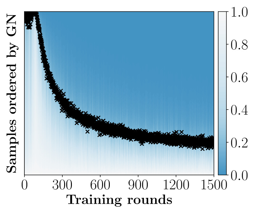
(a) FEMNIST dataset.

(b) Shakespeare dataset.

Figure 1. Ordered gradient norm (GN) of samples from FL training rounds on two different datasets.

Inefficiency of Full Data Training. As in FedAvg (McMahan et al., 2017), most FL approaches let clients to fully train their entire data at a training round. Other approaches that samples a subset of client training data for each round use equal weights on all data (Lai et al., 2021; Fallah et al., 2020; Jiang et al., 2019). However, previous studies in centralized machine learning (Katharopoulos and Fleuret, 2018; Alain et al., 2015; Loshchilov and Hutter, 2015) found that the importance of all samples are not equal; A large portion of samples are learned quickly after few training rounds and could be ignored afterwards. Thus, we conducted an experiment to verify if the same phenomenon also applies in FL and how significant it is. We suspect that the inefficiency problem would be more serious in FL as limited computational resources of mobile clients could be wasted on non-important samples.

In this experiment, we measured the Gradient Norm (GN) of each sample on federated clients to evaluate sample-level contribution on a model update. For each training round, we collected and sorted the GN of each sample from the selected clients. We removed top 5% of samples to avoid evaluating noisy samples and applied min-max scaling to [0.0, 1.0] interval. The experiment ran until the model converged. The results from each dataset are shown in Figure 1(a) and 1(b). Each column of graphs indicates the sorted GN of samples from a training round, where the largest value is located at the bottom. The x-shaped points illustrate where the gradient norm with scaled value of 0.2 exists at each training round.

From both datasets, we observe that the GN of samples are mostly high at the early stage of FL, but only small portion of samples show high GN afterwards, meaning that the number of samples that contribute knowledge to the model are reducing as the training progresses. In FEMNIST dataset, only 6.8% of the samples from early training rounds (round index 0$\sim$150) have less scaled GN value than 0.2, but 80.0% of the samples are less than 0.2 for the last 150 training rounds. Similarly in the Shakespeare dataset, 6.7% of the samples from early training rounds (round index 0$\sim$25) have less scaled GN value than 0.2, but 54.8% of the samples are less than 0.2 for the last 25 training rounds. This result also implies that the samples are not equally important during these FL tasks and current FL approaches could spend large portion of training time for samples that have negligible contribution to the model update.

This experiment motivates to start training with all the samples at the beginning, and then gradually remove samples that the model has already learned. In Section 3.2, we further illustrate how selects a subset of samples of each client at training rounds based on our findings in this experiment.

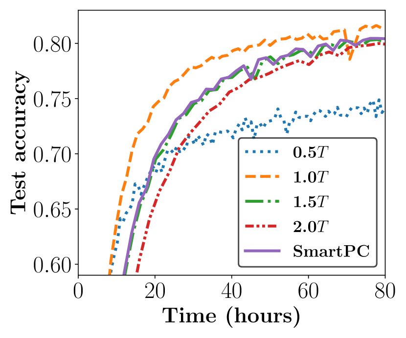
(a) FEMNIST dataset.

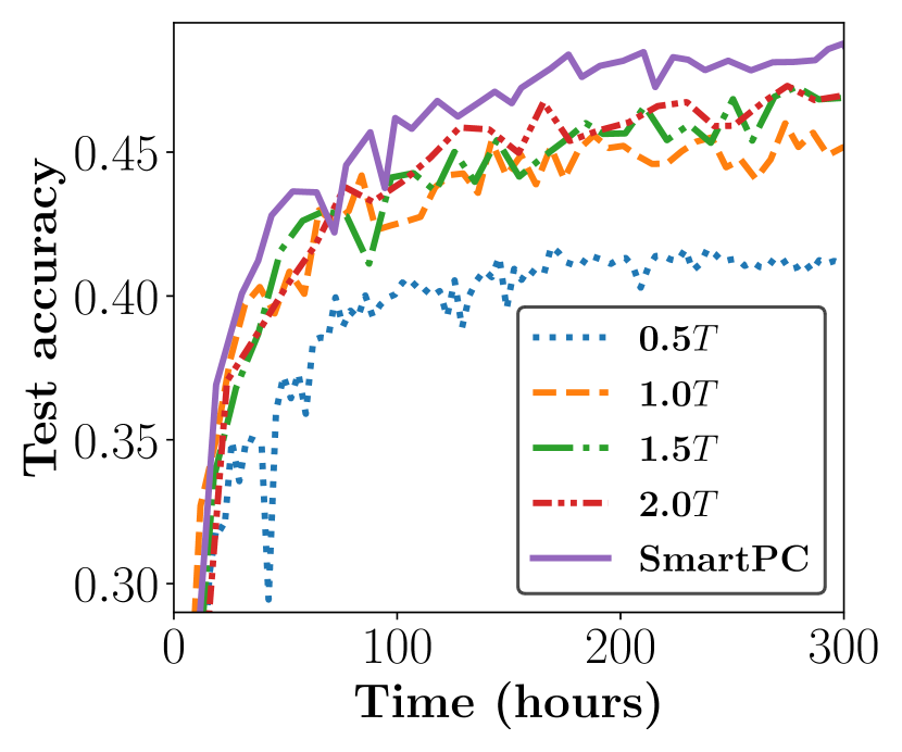
(b) Shakespeare dataset.

Figure 2. FL on two datasets with different deadline configuration methods.

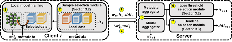
Figure 3. Overview of architecture and its operation in an FL round in seven steps.

Importance of Deadline Selection. While the existence of optimal deadline for achieving shortest training time in FL has been studied (Yang et al., 2021), controlling the deadline for high time-to-accuracy performance has been largely overlooked. To understand the performance of existing deadline configuration methods, we conducted an experiment on the two datasets with SmartPC (Li et al., 2019b) and four different fixed deadlines — 0.5$T$, 1.0$T$, 1.5$T$, and 2.0$T$ — where $T$ indicates the mean of round completion time on every participating client. For SmartPC, we implemented a training round to last until 80% of the clients complete their task, where 80% is suggested by Li et al. (Li et al., 2019b).

Figure 2(a) and  2(b) illustrate the results on two datasets. Our takeaway from this experiment is twofold: (1) The deadline is a significant factor in achieving fast convergence speed and high accuracy, and (2) no single method achieved the best performance for both FL tasks. In FEMNIST dataset, deadline 1.0$T$ achieved the highest final accuracy (.815), while being 43.6%, 47.0% and 77.9% faster than SmartPC, deadline 1.5$T$, and deadline 2.0$T$, respectively, in achieving the test accuracy of .750. On the other hand, in Shakespeare dataset, SmartPC achieved the highest final accuracy (.488) while being 61.7%, 42.8%, and 45.4% faster than deadline 1.0$T$, 1.5$T$, and 2.0$T$, respectively, in achieving the test accuracy of .450. Deadline 0.5$T$ could not achieve high accuracy in either task, as most clients failed to upload their model update within the deadline.

In a training round of FL, the computation time has been shown to be the bottleneck (Wang et al., 2020a; Pilla, 2021; Yang et al., 2021). As the amount of client computation changes with the sample selection of , finding an optimal deadline could be an important problem in achieving high time-to-accuracy performance. To this end, in Section 3.3, we propose how finds the optimal deadline for each training round for efficient FL on heterogeneous clients.

3.

3.1. Overview

For each round of FL, adaptively selects the client training data and controls the deadline to achieve high time-to-accuracy performance. We first provide an overview of how operates in an FL round and then describe how each component of is designed.

Figure 3 depicts the architecture during an FL round. The main functionality of is to actively control two variables for each round: loss threshold ($lt$) and deadline ($ddl$). The loss threshold works as a parameter that determines each client’s training data (Section 3.2) and the deadline determines the round termination time. The numbers inside a circle show the seven steps of an FL round with .

The server first transmits the current model weights $\displaystyle{w}_{R}$, the loss threshold $lt_{R}$, and the deadline $ddl_{R}$ (R indicates the R-th round) to the selected clients of the round (Step 1). The sample selection module at each client selects the partial training data with the received loss threshold (Step 2) and trains the received model (Step 3). The client transmits the model update and the metadata collected from the sample selection and model training (Step 4), and the server aggregates these responses from all clients (Step 5). Based on the metadata from clients, the loss threshold selection module and the deadline selection module each selects the loss threshold $lt_{R+1}$ and the deadline $ddl_{R+1}$ for the next round (Steps 6 and 7).

Challenges: We aim to address the following challenges to realize :

1. Sample selection without accuracy drop: Simply reducing the training data with random sampling could result in degradation of model accuracy due to the decreased statistical utility. should thus prioritize samples based on their statistical utility.

2. Privacy-preserving sample selection in FL: While we aim to select an optimal set of client training data for each round, requiring up-to-date sample-level information from clients could harm the privacy guarantee of FL. should select client training samples without collecting privacy-invasive information from clients.

3. Predicting optimal deadline with varying data: As computation could be the bottleneck of an FL round (Wang et al., 2020b; Pilla, 2021; Yang et al., 2021), applying sample selection strategy of might greatly change the round completion time of clients. should adaptively predict the optimal deadline based on the sample selection status of heterogeneous clients for each round of FL.

3.2. Client Sample Selection

In Section 2.2, we observed that existing FL methods consume large portion of time to train samples that contribute only small gradient to the model. As these samples are quickly learned after few rounds, we design to start training with all samples and gradually remove already-learned samples. This enables to efficiently focus on more important samples at each round while optimizing the training process of FL. However, implementing such design in FL is non-trivial as the following question needs to be addressed: How should distinguish between important and non-important samples at each stage of FL?

A straightforward solution is to collect every sample-level importance information from all clients to a server at each round, and derive a criteria that determines more important samples to a current model. However, such approach is hardly applicable in FL as sharing information of every sample could break the privacy guarantee of FL and reveal the clients’ data. This approach also incurs significant network overhead in communicating all sample’s information at each round. An alternative approach is to have clients classify more important samples within their local data without exposing any information. However, as client data distributions are heterogeneous in FL (McMahan et al., 2017; Wu et al., 2020; Li et al., 2020a; Zhao et al., 2018; Li et al., 2021a), clients could struggle to determine important samples without knowing the global data distribution.

To address this issue, we propose a client-server coordination to maintain a loss threshold variable, which enables clients to effectively select important samples without exposing private sample-level information. actively controls the loss threshold based on the collected metadata from clients with loss threshold selection module, where the metadata consists of differentially-private statistics of sample-level information.

Note that uses the loss of a sample to measure the statistical utility (and thus the importance) of a sample to the current model, similar to Importance Sampling (Loshchilov and Hutter, 2015; Schaul et al., 2016). While other studies have also leveraged gradient norm or gradient norm upper bound (Katharopoulos and Fleuret, 2018; Alain et al., 2015; Li et al., 2021d) to achieve the same goal, we use loss as it is more widely applicable to FL tasks with non gradient-based optimizations (Rios and Sahinidis, 2013).

3.2.1. Sample selection module

Algorithm 1 Client $i$ at $R$-th round: Sample selection

1:func SelectSample($D^{i}$, $B^{i}$, $loss^{i}$, $lt_{R}$, $ddl_{R}$, $\displaystyle{w}_{R}$, $p$, $E$)

2:     $S\leftarrow$ maxTrainableSize$(mean(B^{i}),ddl_{R},E)$

3:     if $S\geq len(D^{i})$ then

4:         $D^{i}_{R}\leftarrow D^{i}$

5:     else

6:         $D^{i}_{R},OT^{i},UT^{i}\leftarrow\emptyset$

7:         for $x\leftarrow 1$ to $len(D^{i})$ do

8:              if $loss^{i}[x]\geq\displaystyle lt_{R}$ then $OT^{i}.insert(D^{i}[x])$

9:              else $UT^{i}.insert(D^{i}[x])$          

10:         $L\leftarrow max(S,len(OT^{i}))$

11:         $D^{\prime}\leftarrow$ randSample$(OT^{i},L\cdot p))$

12:         $D^{\prime\prime}\leftarrow$ randSample$(UT^{i},L\cdot(1-p))$      

13:     $D^{i}_{R}\leftarrow$concatenate$(D^{\prime},D^{\prime\prime})$

14:     return $D^{i}_{R}$

Algorithm 1 describes how the sample selection module of a client selects the samples at each round after it receives the loss threshold from the server. Let us assume that client $i$’s sample selection module is working at round $R$, with a given loss threshold $lt_{R}$.

First, the module measures if a sample selection on a client is required for this round — i.e., it measures if a client is fast enough to train its full dataset within the given deadline $ddl_{R}$. While makes clients focus on more important samples for efficient training, it allows clients to fully utilize its statistical utility if feasible. To this end, we calculate the maximum number of samples $S$ which client $i$ can train for $E$ epochs before the deadline, and verify if it is larger than the size of the client dataset $D^{i}$ (Line 2 - 4). As the computational ability of a client can change according to the device runtime conditions (Yang et al., 2020), collects the batch training latency of a client as $B^{i}$ during FL and uses the mean latency to estimate the max samples it can process. To calculate the mean latency from the first round, asks clients to sample the latency for $k$ times before FL begins. We used 10 for $k$ in our evaluation.

If the client $i$ is incapable of training its full dataset, the sample selection module determines which samples to train at the FL round by using the list of sample loss ($loss^{i}$). The loss list shows the statistical utility of all samples on the current model. While such loss list could be obtained by inferring all samples on up-to-date model at each round, it requires additional forward pass latency that could degrade the time-to-accuracy performance. Therefore, clients of perform whole-dataset forward pass only once when they are first selected at a round to generate a loss list. Then, whenever they train the subset of data, they update the loss values of selected samples that are obtained from the training procedure. We discuss the trade-off between latency reduction and obtaining up-to-date information in Section 5.

selects client samples based on the list of sample loss as follows: First, it divides client i’s samples into two groups: Under-Threshold ($UT^{i}$) and Over-Threshold ($OT^{i}$). Samples that have smaller loss than the loss threshold $lt_{R}$ are put in $UT^{i}$ and otherwise in $OT^{i}$ (Line 7 - 9). We regard samples in $OT^{i}$ to be more important samples in training the current model and prioritize them in sample selection. We sample $L\cdot p$ samples from $OT^{i}$ and $L\cdot(1-p)$ samples from $UT^{i}$ where $L$ indicates the number of selected samples and $p$ is a parameter in an interval of [0.5, 1.0] (Line 10 - 12). The intuition of sampling a portion of data from $UT^{i}$ is to avoid catastrophic forgetting (Kirkpatrick et al., 2017; Yoon et al., 2021) of the model on already-learned samples.

The number of selected samples, $L$, is determined as the number of samples in $OT^{i}$ ($len(OT^{i})$). The loss threshold gradually increases (explained in Section 3.2.2), which allows clients to efficiently focus on samples with high statistical utility. However, if $S$ is larger than $len(OT^{i})$, a client instead uses $S$ to maximize the statistical utility within the deadline (Line 10). As is built on top of Prox (Li et al., 2020a) that allows clients to train less number of epochs, clients with $S$ less than $len(OT^{i})$ could still contribute to the model update.

3.2.2. Loss threshold selection module

Algorithm 2 $lt$ selection for next ($R+1$)-th round

1:func SelectLossThreshold($LLow_{R}$, $LHigh_{R}$, $ltr$)

2:     $ll\leftarrow min(LLow_{R})$

3:     $lh\leftarrow mean(LHigh_{R})$

4:     $lt_{R+1}\leftarrow ll+(lh-ll)\cdot ltr$

5:     return $lt_{R+1}$

The loss threshold selection module determines a loss threshold that effectively distinguishes the important and non-important samples. As the loss distribution of samples changes as FL proceeds, it is essential for the module to be knowledgeable of the current distribution. To respect privacy, the server collects few statistical information from the loss list of clients as a metadata at the end of each round. Specifically, client $i$ at the $R$-th round provides $LLow^{i}_{R}$ and $LHigh^{i}_{R}$ values to the server, which indicate the low and high loss value of its current samples, respectively. We use the min loss value as $LLow^{i}_{R}$ and use 80% percentile loss from the list as $LHigh^{i}_{R}$ instead of the max value, as noisy samples could have abnormally high loss (Song et al., 2020) and make to misjudge the loss distribution. As such values directly indicate a loss value of a specific sample, we apply Gaussian noise to the values to protect user privacy, as in differential privacy (Lai et al., 2021; McMahan et al., 2018; Wei et al., 2020). These values from clients get further aggregated on the server into a list as $LLow_{R}$ and $LHigh_{R}$. We report the performance of when different levels of noise is applied in Section 4.3.

With these metadata, the loss threshold selection module selects a loss threshold as described in Lines 1 - 5 in Algorithm 2. The module measures the loss low value ($ll$) and loss high value ($lh$) to estimate the current range of sample loss values of the clients (Lines 2 and  3). The module then outputs the loss threshold of the next round ($R+1$) with variable loss threshold ratio ($ltr$), which calculates the linear interpolation between $ll$ and $lh$ (Line 4) as $lt_{R+1}\leftarrow ll+(lh-ll)\cdot ltr$. The loss threshold ratio $(ltr)$ enables to start training with all samples and gradually remove already-learned samples. initialize $ltr$ as 0.0 and gradually increases the value by loss threshold step size $(lss)$ as shown in Algorithm 3. Note that the deadline ratio $(ddlr)$, which controls the deadline of each round (described in Section 3.3), is also controlled with $ltr$.

To control $ltr$ and $ddlr$, evaluates the benefit of the current configuration (loss threshold and deadline) at each round based on the statistical utility. For the $R$-th round, it is defined as $U_{R}\leftarrow\frac{LSum_{R}}{L_{R}\cdot ddl_{R}}$ where $LSum_{R}$ is the loss sum of the selected samples, $L_{R}$ is the sum of the number of selected samples, and $ddl_{R}$ is the chosen deadline for the round. Note that $LSum_{R}$ and $L_{R}$ are calculated only from the clients who completed their task and succeeded in sending the model updates. The calculated $U_{R}$ value is added to the list $U$. compares the $U_{R}$ values in the past rounds to the recent rounds (Line 5). If the past rounds have higher value than the recent rounds, considers the model training to be stable and increases the $ltr$ value by $lss$ to further optimize the training process (Line 6). Otherwise, decreases the $ltr$ value by $lss$ (Line 9). Note that $ddlr$, which is initialized as 1.0, is controlled in opposite direction with $dss$ (Lines 7 and  10). Such control of $ltr$ and $ddlr$ happens every $w$ round (Line 4).

Algorithm 3 $ltr$ and $ddlr$ control at $R$-th round

1:func Ctrl($U$, $LSum_{R}$, $L_{R}$, $ddl_{R}$, $ltr$, $ddlr$, $lss$, $dss$, $w$)

2:     $U_{R}\leftarrow\frac{LSum_{R}}{L_{R}\cdot ddl_{R}}$

3:     $U.insert(U_{R})$

4:     if $R\bmod w\equiv 0$ then

5:         if $\sum U(R-2w:R-w)>\sum U(R-w:R)$ then

6:              $ltr\leftarrow$min$(ltr+lss,1.0)$

7:              $ddlr\leftarrow$max$(ddlr-dss,0.0)$

8:         else

9:              $ltr\leftarrow$max$(ltr-lss,0.0)$

10:              $ddlr\leftarrow$min$(ddlr+dss,1.0)$                

11:     return $ltr$, $ddlr$

3.2.3. Client selection with sample selection

Researchers have studied on how to select a group of clients for a training round to optimize convergence speed and model performance in heterogeneous FL (Lai et al., 2021; Cho et al., 2020b, a). While these approaches prioritize clients with higher statistical utility from the data, applying them along with is non-trivial as the samples are dynamically selected with the loss threshold. To address this issue, we propose a new formulation to calculate the statistical utility of a client $i$ along with the sample selection strategy of as follows:

$$StatUtil(i)\leftarrow\lvert len(OT^{i})\rvert\sqrt{\frac{1}{\lvert len(OT^{i})\rvert}\sum_{s\in OT^{i}}Loss(s)^{2}}.$$

This is based on the formulation of statistical utility of state-of-the-art client selection method (Lai et al., 2021), which we only calculate the statistical utility from the $OT^{i}$ group. Thus, the sum of loss squares in $OT^{i}$, $\sum_{s\in OT^{i}}Loss(s)^{2}$ and the number of samples in $OT^{i}$, $len(OT^{i})$ are also collected from clients as a differentially-private metadata.

3.3. Adaptive Deadline Control

We explain how finds an optimal deadline for each round when the clients’ training time changes with the sample selection.

3.3.1. Efficiency of a deadline

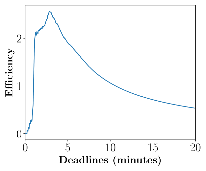
(a) FEMNIST dataset.

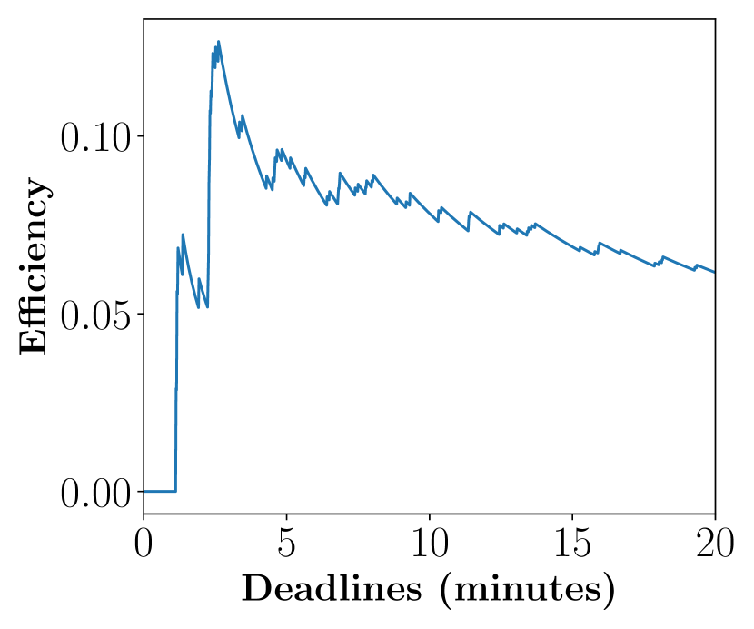
(b) Shakespeare dataset.

Figure 4. Deadline efficiency (DDL-E) evaluation on different deadlines on two FL tasks.

In order to find the best deadline for each round, we define a metric named deadline efficiency (DDL-E) for deadline $t$ as follows:

$$DDL\text{-}E(t)\leftarrow\frac{\text{\# of completed clients before }t}{t}.$$

Our definition of DDL-E formulates the benefit of using deadline $t$ by measuring the amount of completed clients per time. Finding a deadline with high DDL-E value allows the system to avoid choosing too long or too short deadlines. Setting a long deadline with a large $t$ value would have more completed clients but have low efficiency. On the other hand, configuring an extremely short deadline with a small $t$ would result in almost no completed clients and low efficiency.

To understand how DDL-E is distributed at different deadlines at FL task, we profiled the DDL-E based on a large-scale smartphone dataset (Yang et al., 2021). It contains the downlink and uplink network connectivity data and the model training latency data from real-world clients using heterogeneous hardware. We measured the DDL-E for deadlines in range of $[1sec,1200sec]$ on two FL tasks: FEMNIST and Shakespeare.

Figure 4 presents the DDL-E measurements on two FL tasks. From both tasks, we observe that there exists a specific deadline that shows the peak DDL-E value. From the FEMNIST dataset, $t=172$ seconds shows the max efficiency with DDL-E value of $2.57$, while in the Shakespeare dataset, $t=157$ seconds shows the max efficiency with DDL-E value of $0.13$. The distribution shape of DDL-E values showing sharp peak around the max value implies that finding an optimal deadline for FL with could enable more completed clients and improved convergence speed.

Algorithm 4 $ddl$ selection for next ($R+1$)-th round

1:func FindPeakDDL-E($\{DL^{i},UL^{i},B^{i}\}_{i=1}^{N},numEpoch$)

2:     $completeTime\leftarrow\emptyset$

3:     $DDL\text{-}E\leftarrow\emptyset$ $\triangleright$ initialize a list of DDL-E values

4:     $c\leftarrow 0$

5:     $t\leftarrow 1$

6:     for $i\leftarrow 1$ to $N$ do

7:         $T_{network}\leftarrow mean(DL^{i})+mean(UL^{i})$

8:         $T_{train}\leftarrow$ getTrainTime$(mean(B^{i}),numEpoch)$

9:         $completeTime.insert(T_{network}+T_{train})$      

10:     while $c\neq N$ do

11:         $c\leftarrow 0$

12:         for $i\leftarrow 1$ to $N$ do

13:              if $t\geq completeTime(i)$ then

14:                  $c\leftarrow c+1$                         

15:         $DDL\text{-}E.insert(\frac{c}{t})$

16:         $t\leftarrow t+1$      

17:     return maxIndex$(DDL\text{-}E)$

18:func SelectDeadline($\{DL^{i},UL^{i},B^{i}\}_{i=0}^{N},E,ddlr$)

19:     $dl\leftarrow$FindPeakDDL-E$(\{DL^{i},UL^{i},B^{i}\}_{i=1}^{N},1)$

20:     $dh\leftarrow$FindPeakDDL-E$(\{DL^{i},UL^{i},B^{i}\}_{i=1}^{N},E)$

21:     $ddl_{R+1}\leftarrow dl+(dh-dl)\cdot ddlr$

22:     return $ddl_{R+1}$

We designed to select a deadline based on finding the best DDL-E values. Lines 1-  17 of Algorithm 4 shows how finds the deadline with max DDL-E value. This is based on the clients’ hardware capability information: for client $i$, they are DownLink speed ($DL^{i}$), UpLink speed ($UL^{i}$), and Batch training latency ($B^{i}$) (Line  1). When there are a total of $N$ clients involved, we assume clients have already profiled $\{DL^{i},UL^{i}\}_{i=1}^{N}$ before FL and collects $\{B^{i},I^{i}\}_{i=1}^{N}$ during FL. first iterates over N clients to measure their completion time with the mean value of $\{DL^{i},UL^{i},B^{i}\}_{i=1}^{N}$ (Lines 6-  9). then measures the DDL-E from the smallest deadline $t$ (we use $t=1sec$) and increments $t$ until all clients complete before $t$ (Lines 10- 16) and outputs the deadline with the max DDL-E value (Line 17).

As different subset of clients are selected for each round, finds the max DDL-E value among the selected clients of each round. Moreover, as clients use different size of training data with sample selection, we estimate the training time of client $i$ (getTrainTime from Line 8) as follows:

$$\frac{len(OT^{i})-1}{batchSize}\cdot mean(B^{i})\cdot numEpoch.$$

We use the length of $OT^{i}$ in measuring the training time of a client to reflect the number of samples being selected. This allows to reliably find the deadline with the best DDL-E along with the sample selection strategy.

3.3.2. Deadline selection module

The deadline selection module of determines the deadline that optimizes the training process and convergence speed. The module selects the deadline as shown in Lines 18 - 22 of Algorithm 2. The module measures deadline low value $dl$ and deadline high value $dh$, which are the deadlines with the max DDL-E value when clients are running 1 epoch and $E$ epochs, respectively (Lines 19 and  20).

The module then outputs the deadline of the next round (R+1) with parameter deadline ratio ($ddlr$) that calculates the linear interpolation between $dl$ and $dh$ (Line 21) as $ddl_{R+1}\leftarrow dl+(dh-dl)\cdot ddlr$. The reason of selecting a value between $dl$ and $dh$ is because is built on top of Prox (Li et al., 2020a) that allows clients to train various number of epochs within the deadline. With an aim to optimize the training efficiency, initially configures $ddlr$ as 1.0 and gradually decreases the value by the parameter $dss$, as explained in Section 3.2.2.

3.4. Collaboration with FL Methods

One advantage of is its applicability to orthogonal FL approaches that do not perform sample selection on clients or control the deadline. Applying could be achieved by simply adding the sample selection and deadline control strategies on top of other methods. We demonstrate the collaboration capability of with its implementation on top of three existing FL methods and improved performances in Section 4.5.

Some recent FL approaches, such as Oort (Lai et al., 2021), use one batch instead of the full dataset for training in each local epoch, making them non-trivial to be directly integrated with . To address this issue, we propose OortBalancer, which is built on top of Oort, where the sample selection strategy of is adopted with one adjustment: $L$ from Algorithm 1 is fixed to the batch size. Intuitively, while Oort trains one randomly selected batch for each local epoch, OortBalancer selects samples for one batch that focuses on more important samples and thereby optimizes the training process. We demonstrate the performance of OortBalancer in Section 4.5 as one of the three examples of collaboration.

4. Evaluation

We evaluate to answer the following key questions: 1) How much performance improvement (in terms of time-to-accuracy and model accuracy) does achieves over existing FL methods? 2) How sensitive is with different choice of parameters? 3) How much performance improvement does each component of achieves? 4) How does perform when it jointly operates with orthogonal FL approaches?

4.1. Experimental Setup

Table 1. Speedup and accuracy on five datasets with the real-world user data.

Task	CV				NLP				HAR
Dataset	FEMNIST		Celeba		Reddit		Shakespeare		UCI-HAR
Methods	Speedup	Acc.	Speedup	Acc.	Speedup	Acc.	Speedup	Acc.	Speedup	Acc.
FedAvg+1$T$	1.00$\pm$0.00	.796$\pm$.007	0.97$\pm$0.05	.851$\pm$.005	0.08$\pm$0.12	.090$\pm$.001	0.24$\pm$0.22	.399$\pm$.020	0.49$\pm$0.36	.814$\pm$.029
FedAvg+2$T$	0.59$\pm$0.01	.763$\pm$.009	0.59$\pm$0.04	.824$\pm$.010	0.58$\pm$0.07	.104$\pm$.000	0.39$\pm$0.10	.373$\pm$.046	0.68$\pm$0.07	.819$\pm$.014
FedAvg+SPC	0.71$\pm$0.02	.777$\pm$.004	0.80$\pm$0.14	.829$\pm$.013	0.87$\pm$0.08	.112$\pm$.001	0.56$\pm$0.10	.416$\pm$.017	0.91$\pm$0.13	.840$\pm$.016
FedAvg+WFA	0.33$\pm$0.20	.594$\pm$.205	0.54$\pm$0.04	.813$\pm$.020	1.00$\pm$0.00	.113$\pm$.001	1.00$\pm$0.00	.439$\pm$.017	0.68$\pm$0.07	.819$\pm$.014
Prox+1$T$	0.99$\pm$0.02	.795$\pm$.008	1.05$\pm$0.03	.855$\pm$.002	2.87$\pm$0.43	.121$\pm$.005	1.14$\pm$0.16	.476$\pm$.003	0.96$\pm$0.09	.849$\pm$.008
Prox+2$T$	0.65$\pm$0.02	.767$\pm$.006	0.75$\pm$0.04	.833$\pm$.010	3.63$\pm$0.43	.127$\pm$.005	1.00$\pm$0.14	.457$\pm$.003	0.68$\pm$0.07	.819$\pm$.014
SampleSelection	1.01$\pm$0.02	.799$\pm$.006	1.03$\pm$0.06	.852$\pm$.002	1.52$\pm$0.38	.118$\pm$.001	0.85$\pm$0.24	.439$\pm$.021	0.90$\pm$0.05	.845$\pm$.008
	1.57$\pm$0.03	.815$\pm$.006	1.43$\pm$0.07	.862$\pm$.006	4.48$\pm$0.23	.146$\pm$.001	1.20$\pm$0.10	.489$\pm$.004	1.56$\pm$0.28	.855$\pm$.034
-A	1.60$\pm$0.06	.820$\pm$.003	1.52$\pm$0.07	.873$\pm$.004	4.08$\pm$0.76	.154$\pm$.000	1.31$\pm$0.28	.505$\pm$.004	1.39$\pm$0.43	.893$\pm$.008
-S	1.71$\pm$0.01	.819$\pm$.002	1.67$\pm$0.04	.859$\pm$.006	4.99$\pm$0.42	.148$\pm$.003	1.83$\pm$0.14	.488$\pm$.001	1.98$\pm$0.48	.863$\pm$.010

Implementation. We developed on FLASH (Yang et al., 2021), a heterogeneity-aware benchmarking framework for FL based on LEAF (Caldas et al., 2018). FLASH provides a simulation of heterogeneous computational capabilities and network connectivity from a large-scale real-world trace dataset collected over 136k smartphones that span one thousand types of devices. We implement with the state-of-the-art FL aggregation method Prox (Li et al., 2020a). Our implementation is based on Python 3.6 and TensorFlow 1.14 with 2,062 lines of code on top of FLASH. The source code of our implementation are available at https://github.com/jaemin-shin/FedBalancer.

Datasets. To simulate FL tasks in our evaluation, we use five datasets that contain data generated by real-world users, which are categorized in three different domains as follows:

• Computer Vision (CV): For CV, we evaluated on two image recognition datasets: FEMNIST (Cohen et al., 2017) and Celeba (Liu et al., 2015). FEMNIST dataset contains images of handwritten digits and characters from 712 users with total 157,132 samples. Celeba dataset contains face attributes of 915 users with 19,923 samples. We use CNN models for both datasets as in previous work (Yang et al., 2021).

• Natural Language Processing (NLP): We evaluate on two NLP tasks each on different dataset: next-word prediction on Reddit (Caldas et al., 2018) dataset and next-character prediction on Shakespeare (Shakespeare, 2014) dataset. The Reddit dataset contains reddit posts from 813 users with 32,680 samples, and the Shakespeare dataset contains 845,231 samples separated into 171 users. We use LSTM models for both datasets as in previous work (Yang et al., 2021).

• Human Activity Recognition (HAR): We use UCI-HAR dataset (Anguita et al., 2013) that contains six types of activity data on accelerometer and gyroscope from 30 users with 10,299 samples. As in previous work, we use CNN models (Ek et al., 2021).

Metrics. As in the previous work (Lai et al., 2021) that evaluated on heterogeneous FL clients, we mainly evaluate time-to-accuracy performance and final model accuracy on the experiments. Here, the time-to-accuracy performance indicates the wall clock time that is required for a model training task to reach an accuracy target. We repeat each experiment for three times with different random seeds and report the average and standard deviation of these evaluation metrics.

Baselines. We use the following list of approaches as a baseline to compare with in our evaluation:

• Aggregation algorithms: We use FedAvg (McMahan et al., 2017) and Prox (Li et al., 2020a), the most widely used aggregation algorithms for FL. Prox offers an optimizer with convergence guarantee on heterogeneous clients, while allowing clients to train various number of local epochs within the deadline. For the $\mu$ parameter of Prox, we tested $\mu$ in $\{0.0,0.001,0.01,$ $0.1,1.0\}$ as suggested by the paper and pick one with the best final accuracy. All the datasets showed the best accuracy with $0.0$ except Celeba with $0.1$.

• Deadline configuration methods: We use four different deadline configuration methods in the evaluation. We configure two different fixed deadlines as a baseline, which are $1T$ and $2T$. Before the training begins, we sample the round completion time of all participating clients and calculate the mean value as $T$. Thus, $2T$ uses double of that mean value as a fixed deadline. We also adopt SmartPC (SPC) (Li et al., 2019b), and implemented it to involve the certain portion $U_{required}$ of users to complete at a training round. As suggested in the paper, we use 80% for $U_{required}$. Lastly, we use a method that waits every client to finish a round, which we named as WaitForAll (WFA).

• Sample selection method: We implement the baseline sample selection method that is a combination of the following: (1) We determined how many samples to select based on FedSS (Cai et al., 2020), which controls the training dataset size on clients with larger datasets for each training round. (2) There were several approaches that propose which samples to select based on loss (Loshchilov and Hutter, 2015; Schaul et al., 2016), gradient (Alain et al., 2015), or gradient norm upper bound (Katharopoulos and Fleuret, 2018; Li et al., 2021d) of samples. As in , we use loss to select samples for the baseline experiment.

For baseline experiments, we use the combination of the aggregation algorithms and the deadline configuration methods of above. We do not test SPC with Prox as it is nontrivial to accept stragglers’ model update with less number of epochs when $U_{required}$ users complete a training round. Moreover, we do not test WFA with Prox as it is identical with FedAvg when $\mu=0$, which is used by most datasets. We test the sample selection method with the best performing deadline configuration methods with Prox, which is Prox+$2T$ for Reddit dataset and Prof+$1T$ otherwise.

Table 2. $\{w,lss,dss,p\}$ parameters from the experiments in Table 1. Parameters with forward slashes indicate the different parameters from the multiple runs of experiments with three different random seeds.

					-A				-S
	$w$	$lss$	$dss$	$p$	$w$	$lss$	$dss$	$p$	$w$	$lss$	$dss$	$p$
FEMNIST					20	0.01/0.1/0.1	0.10	1.00	20	0.05/0.05/0.01	0.25/0.1/0.05	1.00
Celeba					20/5/5	0.05/0.1/0.01	0.1/0.1/0.05	1.00/0.75/1.00	20/20/5	0.01/0.01/0.1	0.1/0.1/0.25	1.00/1.00/0.75
Reddit	20	0.05	0.05	1.00	5/20/20	0.01	0.1/0.25/0.1	1.00	5	0.1	0.25/0.1/0.05	0.75
Shakespeare					5	0.01/0.05/0.01	0.1/0.25/0.25	1/0.75/1	5/20/5	0.05/0.01/0.1	0.1/0.05/0.1	0.75
UCI-HAR					5/5/20	0.1/0.01/0.05	0.1/0.1/0.25	1/1/0.75	5	0.1/0.1/0.05	0.25	0.75/0.75/1

Table 3. Speedup and accuracy on different choice of parameters.

Parameter		$w$		$lss$			$dss$			$p$
		$5$	$20$	$0.01$	$0.05$	$0.10$	$0.05$	$0.10$	$0.25$	$0.75$	$1.00$
FEMNIST	Speedup	1.39$\pm$0.16	1.52$\pm$0.15	1.37$\pm$0.15	1.49$\pm$0.18	1.50$\pm$0.14	1.54$\pm$0.07	1.47$\pm$0.16	1.35$\pm$0.18	1.41$\pm$0.15	1.50$\pm$0.17
	Accuracy	.813$\pm$.005	.816$\pm$.004	.813$\pm$.004	.815$\pm$.006	.816$\pm$.006	.817$\pm$.003	.814$\pm$.004	.812$\pm$.005	.814$\pm$.004	.815$\pm$.005
Reddit	Speedup	3.40$\pm$0.53	3.70$\pm$0.23	3.60$\pm$0.29	3.61$\pm$0.31	3.44$\pm$0.61	3.66$\pm$0.44	3.60$\pm$0.33	3.40$\pm$0.48	3.71$\pm$0.30	3.39$\pm$0.49
	Accuracy	.146$\pm$.007	.147$\pm$.003	.150$\pm$.002	.147$\pm$.002	.143$\pm$.008	.147$\pm$.004	.146$\pm$.007	.147$\pm$.005	.149$\pm$.002	.144$\pm$.007

Method. We first ran FedAvg+$1T$ on five datasets until convergence, with the number of rounds that are suggested by previous works (Caldas et al., 2018; Yang et al., 2021; Ek et al., 2021; Sozinov et al., 2018): 1000, 100, 600, 40, and 50 rounds for FEMNIST, Celeba, Reddit, Shakespeare, and UCI-HAR. Based on the user trace data of FLASH, we measured the wall clock time which FedAvg+$1T$ ran for each dataset, and ran experiments with other baselines and until the same wall clock time. Among the four FedAvg baselines, we pick the one with best accuracy for each dataset and configure it as the target accuracy of that task. Then, we measured the speedup of other methods in achieving the target accuracy and their final model accuracy achieved within the same wall clock time.

We tested the following combination of parameters for : $w$ in $\{5,20\}$, $lss$ in $\{0.01,0.05,0.10\}$, $dss$ in $\{$0.05, 0.10, 0.25$\}$, and $p$ in $\{0.75,1.00\}$. Among the results, we report the performance of with only one set of parameter: $\{w,lss,dss,p\}=\{20,0.05,0.05,1.00\}$. This is a set of parameters that we recommend FL developers to try with their task when they are not knowledgeable of which parameter performs the best. We used this parameter for all the experiments in Section 4. In Section 4.2, we also report the parameter set with the best final accuracy for each dataset as -A and the best speedup as -S to demonstrate the maximum performance could achieve.

Other configurations. As in previous study (Yang et al., 2021), we use batch size of 100 for Shakespeare and 10 for rest of the datasets. We select 100 clients at each round for datasets with more than 500 users, and otherwise select 10 users for Shakespeare and 5 users for UCI-HAR. We configured the clients to train five local epochs per round. We use learning rate of 0.001 for FEMNIST and Celeba, 2 for Reddit, 0.8 for Shakespeare, and 0.005 for UCI-HAR.

4.2. Speedup and Accuracy on Five FL Tasks

Table 1 shows the performance of on five datasets compared with the baseline methods, and Table 2 shows the parameters used for , -A, and -S for each dataset. We observed that shows improved time-to-accuracy performance over the baselines on every dataset: reaches the target accuracy 1.43$\sim$1.57$\times$ faster than the FedAvg-based baselines on CV datasets, 1.36$\sim$1.58$\times$ faster than the Prox-based baselines, and 1.39$\sim$1.55$\times$ faster than the SampleSelection baseline. achieves 1.20$\sim$4.48$\times$ speedup and 1.05$\sim$1.23$\times$ speedup compared with the FedAvg and Prox-based methods respectively, while achieving 1.41$\sim$2.95$\times$ speedup over the SampleSelection baseline on NLP datasets. achieves speedup of 1.56$\times$, 1.63$\times$, and 1.73$\times$ compared with FedAvg, Prox, and SampleSelection baselines on a HAR dataset, respectively.

We noticed that consistently shows high time-to-accuracy performance on all datasets, while the performance of baselines was inconsistent across datasets. For example, among FedAvg-based baselines, FedAvg+$1T$ shows the best time-to-accuracy performance on CV tasks but shows extremely low performance on NLP tasks. In contrast, FedAvg+WFA shows the best time-to-accuracy performance on NLP tasks among FedAvg-based baselines but shows low performance on CV tasks. In UCI-HAR, FedAvg+$1T$ and FedAvg+SPC resulted in the best performance at different experiments with different random seeds. Prox+$1T$ shows the best performance among baselines on Celeba, Shakespeare, and UCI-HAR, but shows worse performance than SampleSelection and Prox+$2T$ on FEMNIST and Reddit respectively.

We observed that achieves this improvement of time-to-accuracy performance without sacrificing model accuracy; in terms of the final model accuracy, showed improvement over the baselines on all datasets. Compared to the FedAvg-based methods, achieved 1.1$\sim$5.0% accuracy improvement on different datasets. achieved 0.6$\sim$3.2% and 1.0$\sim$5.0% accuracy improvement over Prox-based methods and the Sampleselection baseline. -A, which marks the best accuracy of , also shows time-to-accuracy performance improvement over baselines at all datasets — showing further improvement in speedup on FEMNIST, Celeba, and Shakespeare. On the other hand, -S, which reports the best time-to-accuracy performance of , shows accuracy improvement over baselines at all datasets, with further improvement in accuracy on FEMNIST, Reddit, and UCI-HAR. This suggests that the performance of could be further improved with a carefully selected parameter for an FL task, while the fixed parameter set we recommend still shows improved performance.

4.3. Parameter Sensitivity Analysis

Table 3 shows the time-to-accuracy performance and final accuracy of on different choice of parameters $\{w,lss,dss,p\}$. For each type of parameter, we fixed it to a certain value and averaged the performance from experiments with different combination of other parameters. We used speedup compared to the best FedAvg-based baseline to measure the time-to-accuracy performance. We chose FEMNIST and Reddit to explore the effect of different parameters at different domains of FL tasks (CV and NLP).

For $w$, shows similar final accuracy (81.3% and 81.6%) performance on both of the candidate values on FEMNIST, but reports better time-to-accuracy performance (1.52$\times$ over 1.39$\times$) with $w=20$. On Reddit, $w=20$ showed better speedup (3.71$\times$ over 3.42$\times$) and accuracy (14.8% over 13.3%). In terms of $lss$, achieves faster training and higher accuracy when $lss\geq 0.05$ on FEMNIST, but achieves better performance when $lss\leq 0.05$ on Reddit. With $dss$, performs the better when $dss\leq 0.1$ on both datasets, where both showed the best time-to-accuracy and accuracy with smaller $dss=0.05$. Lastly, performs better with $p=1.00$ on FEMNIST but reports better performance with $p=0.75$ on Reddit. For the different trend of performance with $lss$ and $p$ parameters on two datasets, we suspect that Reddit requires more rounds with data sampled from full dataset in the early stage of training to achieve better performance, and big $lss$ and $p=1.00$ performs worse as it might quickly remove the low-loss samples from training. On the other hand, FEMNIST training performs better with high-loss samples from the early stage of training. This suggests that the best set of parameters could be selected based on how the training at an FL task proceeds.

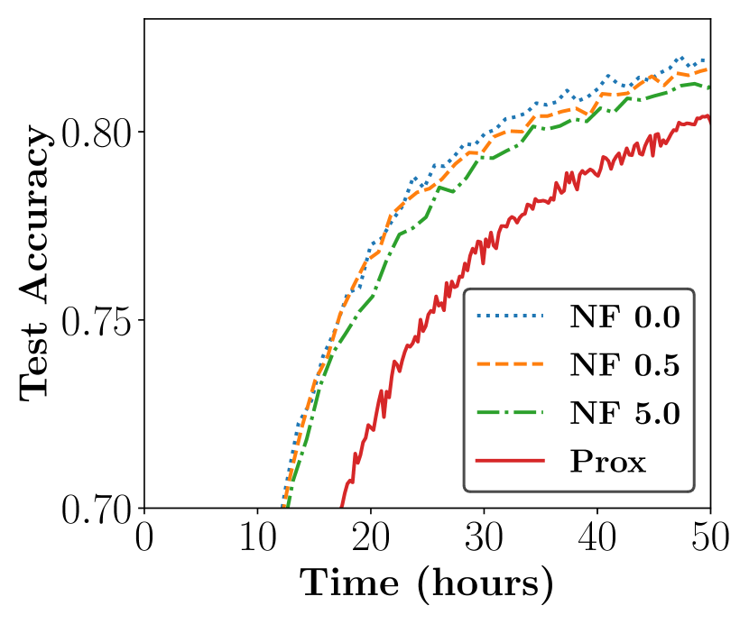
(a) On Different Level of Differential Privacy.

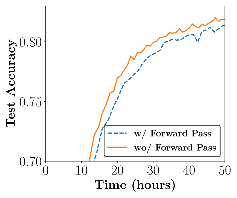
(b) With and Without the Forward Pass at Each Round.

Figure 5. Performance evaluation of with different options on FEMNIST.

Other than the algorithm parameter of , we study the effect of different level of noise on differential privacy that we applied to mask the metadata shared by the clients. Our implementation of differential privacy is based on the previous work (Lai et al., 2021), adding the noise drawn from Gaussian distribution on the metadata, with the mean as zero and the standard deviation as Noise Factor (NF). Figure 5(a) shows the effect of different NFs on the performance of . We observe that the performance of degrades as the NF increases, as NF 0.0 achieves 81.9% accuracy but NF 0.5 and 5.0 each achieves 81.4% and 81.1% accuracy. However, NF 0.5 and 5.0 still achieves better time-to-accuracy performance and accuacy compared to Prox, while NF of 5.0 is considered to be very large noise (Abadi et al., 2016). This result implies that could achieve performance improvement over the baselines while applying the differential privacy.

4.4. Effect of Components

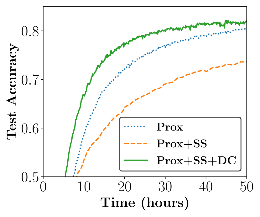
(a) FEMNIST dataset.

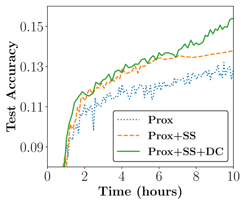
(b) Reddit dataset.

Figure 6. Performance breakdown of into Sample Selection (SS) and Deadline Control (DC).

We conducted an experiment to understand the performance brought by each component of : Sample Selection (SS) and Deadline Control (DC). As is built on top of Prox (Li et al., 2020a), we add the components one by one to observe how the performance changes when each component is introduced.

Figure 6 reports the result of the experiment on FEMNIST and Reddit dataset. On FEMNIST dataset, we observe that the performance drops when SS is introduced, but gets further improved when DC is added. On Reddit dataset, however, the accuracy escalates as each component is added. The reason of performance degradation on FEMNIST with SS is due to the reduced statistical utility trained at each round with the same deadline. In contrast on Reddit dataset, the performance improved with SS as it allowed more clients to successfully send their model updates within the deadline with selected client data. Moreover, we suspect that SS has brought more performance improvement on Reddit than FEMNIST by effectively selecting more important samples and the clients that have such data. The result with DC on both dataset shows its effectiveness with SS in time-to-accuracy performance improvement.

4.5. Collaboration with FL Algorithms

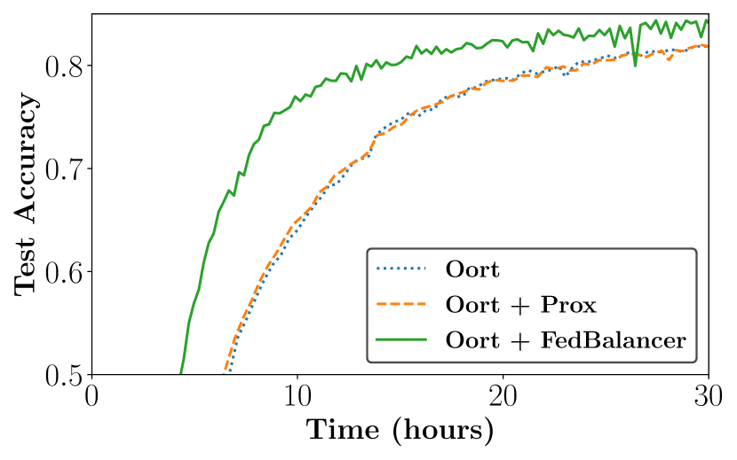
(a) Oort (Lai et al., 2021).

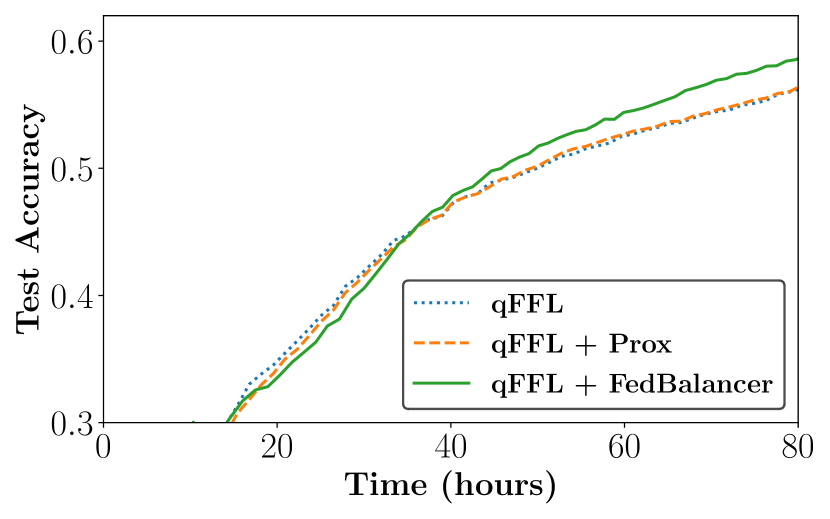
(b) q-FFL (Li et al., 2020b).

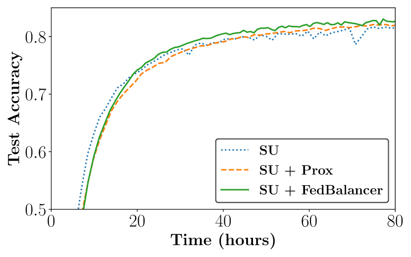
(c) Structured Updates (Konečnỳ et al., 2016).

Figure 7. Collaboration of with three FL algorithms on FEMNIST dataset.

To demonstrate the applicability of on orthogonal FL algorithms, we implement on top of three widely used FL approaches from different categories: Oort (Lai et al., 2021) as a client selection algorithm, q-FFL (Li et al., 2020b) as an aggregation algorithm, and Structured Updates (Konečnỳ et al., 2016) as a gradient compression algorithm. Figure 7 reports the experiment result, which we observe improvement in time-to-accuracy performance and model accuracy from all three cases. Collaboration with achieved 1.84$\times$, 1.19$\times$, and 1.31$\times$ speedup, while achieving 2.6%, 2.5%, 1.7% accuracy improvement on three algorithms respectively. These results suggest that could be implemented on top of various advanced FL algorithms to achieve further performance improvement.

Table 4. Android devices for the testbed experiments.

Builder	Year	Device	Processor	Quantity
Google	2016	Pixel	Snapdragon 821	2
	2017	Pixel 2	Snapdragon 835	1
	2017	Pixel 2 XL	Snapdragon 835	2
	2018	Pixel 3	Snapdragon 845	1
	2020	Pixel 5	Snapdragon 765G	1
Samsung	2016	Galaxy S7	Exynos 8890	1
	2017	Galaxy J7	Exynos 7870	1
	2019	Galaxy Fold	Snapdragon 855	1
Huawei	2015	Nexus 6P	Snapdragon 810	3
	2018	P20 Lite	Kirin 659	1
Motorola	2014	Nexus 6	Snapdragon 805	2
LG	2015	Nexus 5X	Snapdragon 808	4
Essential	2017	Essential Phone	Snapdragon 835	1

4.6. Testbed Experiments with Android Clients

Table 5. Results from the testbed experiments.

Method	Speedup	Accuracy
FedAvg+1T	0.99$\pm$0.03	.852$\pm$.020
FedAvg+2T	0.75$\pm$0.30	.800$\pm$.034
FedAvg+SPC	0.61$\pm$0.35	.849$\pm$.013
FedAvg+WFA	0.92$\pm$0.07	.846$\pm$.007
FedProx+1T	1.03$\pm$0.23	.860$\pm$.007
FedProx+2T	0.90$\pm$0.20	.860$\pm$.013
SampleSelection	0.99$\pm$0.13	.846$\pm$.014
	1.33$\pm$0.08	.885$\pm$.017

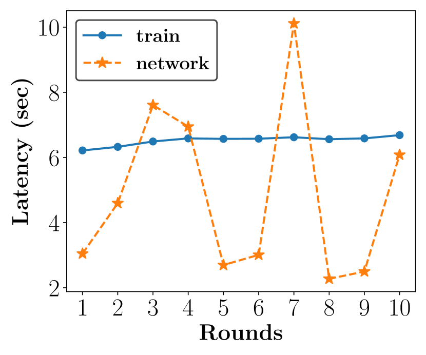
(a) Google Pixel 5.

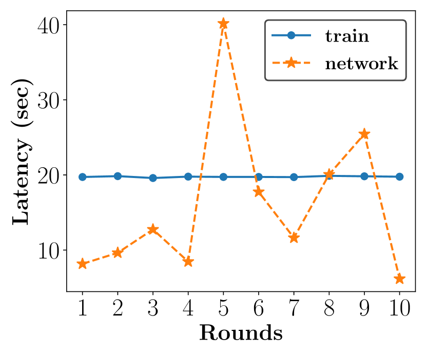
(b) Huawei P20 Lite.

Figure 8. On-device training latency (train) and communication latency (network) on different devices.

We further conducted experiments on Android clients to understand the effectiveness of on real hardware devices. We implemented the server using Flower (Beutel et al., 2020), which is an open-source FL framework that communicates with clients via gRPC (Google Remote Procedure Call) and Protocol Buffers (pro, [n.d.]). We used Ubuntu 18.04 server with Intel Xeon Gold 6254 Processor @ 3.10GHz and 512GB RAM. On-device training on Android devices were implemented with the model personalization feature of Tensorflow Lite (tfl, [n.d.]). We used UCI-HAR dataset and used the same experimental configuration as illustrated in Section 4.1.

For 21 client devices in UCI-HAR experiments, we used 13 different Android models to simulate the hardware heterogeneity in the real-world as illustrated in Table 4. We placed the devices in an office room of a laboratory building, where the devices were connected to a campus Wi-Fi. To configure fixed deadlines for the deadline configuration methods $1T$ and $2T$, we sampled the training round completion time of each device 10 times before the experiments.

Table 5 shows the performance of compared with the baseline methods in our testbed experiments. shows higher time-to-accuracy performance and final model accuracy over the baselines. showed 1.34$\times$ speedup and 3.3% accuracy improvement over the FedAvg-based baselines. also achieved the target accuracy 1.29$\times$ and 1.34$\times$ faster than Prox and SampleSelection baselines, with 2.5% and 3.9% accuracy improvements.

One of the unique challenges we discovered in the testbed experiments was dynamically changing round completion times of the client devices. To further understand the cause of such a phenomenon, we separately sampled the on-device training latency and the communication latency on the client devices at a training round, as shown in Figure 8. Compared with the on-device training latency that remained constant at different rounds, the communication latency showed high variability at each round, showing up to 3.91$\times$ increase over the mean communication latency. Our testbed experiment had higher variability than our previous simulated experiments, as the mean CV (Coefficient of Variance) of communication latency was 1.5$\times$ larger (0.59 over 0.40).

Such variable communication latency affected each FL method differently. For baselines that use fixed deadlines (e.g., 1$T$), clients often failed to send their model updates due to long communication latency. For SmartPC (SPC) and Wait-for-All (WFA) baselines, the server had to wait for a prolonged duration when the clients were experiencing poor network connectivity. As the network conditions were not identical at different experiments, some baselines (FedAvg+2$T$, FedAvg+SPC, Prox+1$T$, and Prox+2$T$) yielded performance with huge variance ($\geq$ 0.20 in speedup). While client failures also negatively affected , it achieved superior time-to-accuracy and accuracy performance over the baselines due to its adaptive deadline configuration with DDL-E measurement on the sampled clients at a training round.

We suspect the variability of the communication latency would be higher in real deployments as users with mobility and unstable network conditions would be involved. Moreover, the impact of variable communication latency would be more significant when we train larger models with ¿100M parameters (e.g., BERT (Devlin et al., 2019)) in FL. As is not designed to actively respond to the network connectivity changes of clients in real-time, we expect could be improved further if the client-side network condition analysis system is integrated to accurately predict the round completion time of selected clients at each round. We leave this as future work.

5. Discussion

Local Epoch Training Policies. While was originally designed for FL based on FedAvg (McMahan et al., 2017) that performs full data training per local epoch of client, recent studies such as Oort (Lai et al., 2021) propose to perform single batch training per local epoch. There are pros and cons in both approaches; single batch training offers more frequent global model update with shorter training time on clients, but this could lead to excessive communication overhead when training large models. Full data training exploits full statistical utility of client data per round, but offers less frequent global model update with longer round. While it is the model developer’s role to determine the option, is readily applicable and improves time-to-accuracy performance on both as we demonstrated in the evaluation.

Effect of Forward Pass at a Client. When selects a clients’ samples, it uses a list of sample loss that is maintained on a client from the beginning of FL, instead of performing a forward pass on the client data at each round. A sample loss at the maintained list is only updated whenever the sample is selected and trained by a client, which may result in containing outdated information. We conducted an experiment to understand the effect of forward pass on performance of , which is shown in Figure 5(b). On FEMNIST dataset, integrating the forward pass with resulted in slower training, which supports our design without the forward pass. This is because that the outdated loss values are generally larger than the newly-updated ones, which encourages to select more diverse samples while prioritizing informative samples.

Robustness of Sample Selection. One of the possible limitation of is that it might perform worse on FL tasks with noisy data, as noisy samples are highly likely to be selected by the sample selection module that prioritizes high loss. As we observed the performance improvement with on five real-world user datasets which may already have certain noise level, we expect would be helpful on most FL tasks. To improve further, we could systematically involve robust training approaches at centralized learning (Shen and Sanghavi, 2019; Roh et al., 2021; Song et al., 2019) to actively deal with noisy data. This is part of our future work.

Potential Bias of Sample Selection. While FedBalancer prioritizes more “informative” samples for training, it might integrate more samples from certain classes or sensitive groups than others, potentially leading to performance degradation on less sampled entities. To address this issue, we could integrate our sample selection strategy with other sample selection or reweighting approaches (Roh et al., 2021; Yan et al., 2022) that are designed to achieve unbiased model training. We leave this as future work.

6. Related Work

We survey closely related work with other than the FL approaches on heterogeneous clients which we discussed earlier in Section 2.2.

Sample Selection in Machine Learning. There are several sample selection approaches in the field of machine learning research that could be arranged in threefold: (1) Curriculum Learning (CL) (Wu et al., 2020; Bengio et al., 2009; Graves et al., 2017; Hacohen and Weinshall, 2019; Huang et al., 2020): CL is a sample ordering technique which trains a network with easier samples in early training stage and gradually increase the difficulty to improve convergence speed and model generalization. However, applying it in FL is challenging as CL require a reference model to determine the difficulty of samples, which hardly exists in FL scenarios. (2) Active Learning (AL) (Settles, 2009; Balcan et al., 2009; Gal et al., 2017; Kirsch et al., 2019): AL is a sample selection technique on unlabeled data, which interactively queries the user to label new data points that is likely to be more informative to the given task. Applying AL in FL could be non-trivial, as the training data is isolated and the labels are known but not shared externally from the clients. (3) Importance Sampling (Katharopoulos and Fleuret, 2018; Alain et al., 2015; Loshchilov and Hutter, 2015; Schaul et al., 2016): Being motivated by the fact that the importance of each training samples is different, researchers have proposed importance sampling techniques to accelerate the model training. While their idea could be brought to FL to prioritize samples during training, determining how many and which samples to use for each training round and when to calculate the sample importance is yet unknown.

Sample Selection in FL. Tuor et al. (Tuor et al., 2020) proposed a scheme that selects relevant clients’ data to the given FL task, but it only selects the dataset before the FL starts. Moreover, it requires an example dataset, which is hardly applicable at FL scenarios where the client data distributions are usually unknown. Li et al. (Li et al., 2021d) proposes how we can prioritize client training samples with higher importance in FL using gradient norm upper bound (Katharopoulos and Fleuret, 2018). However, their approach does not provide how many samples should be selected per each round. While other methods such as FedSS (Cai et al., 2020) determines the amount of client training samples during FL, it does not specify which samples to select, simply adopting random sampling of the data. Moreover, combining FedSS with Li et al. is nontrivial, as FedSS assumes random sampling of the data. Unlike previous approaches, is the first systematic framework that actively determines (1) how many and (2) which samples to select during FL to improve time-to-accuracy performance. We believe such design of enables the use of client sample selection to improve time-to-accuracy performance.

Deadline Control in FL. Determining an optimal deadline has been largely overlooked by previous approaches; only SmartPC determines a deadline to enable a specified proportion of the devices to complete a training round. It assumes that every client uses the same set of data for each round of FL. on the other hand utilizes a new deadline control strategy for FL that enables high convergence speed where client training samples dynamically change during FL due to sample selection.

7. Conclusion

We presented , a systematic FL framework with sample selection for optimized training process. actively selects the samples with high statistical utility through client-server coordination at each FL round without exposing private information of users. To further accelerate FL with our sample selection, we design adaptive deadline control strategy for to predict the optimal deadline for each round with client sample selection. Our evaluation of on five real-world datasets from three different domains reveal that achieves 1.20$\sim$4.48$\times$ speedup over existing FL algorithms with different deadline configuration methods, while improving the model accuracy by 1.1$\sim$5.0%. Our design of is easily applicable on top of orthogonal FL methods, that we demonstrate the joint implementation of with three existing FL algorithms and report the improved time-to-accuracy performance and model accuracy.

- (1)
- pro ([n.d.]) [n.d.]. Protocol Buffers. https://developers.google.com/protocol-buffers/docs/overview. Accessed: 2022-05-17.
- tfl ([n.d.]) [n.d.]. TensorFlow Lite. https://www.tensorflow.org/lite. Accessed: 2022-05-17.
- Abadi et al. (2016) Martin Abadi, Andy Chu, Ian Goodfellow, H. Brendan McMahan, Ilya Mironov, Kunal Talwar, and Li Zhang. 2016. Deep Learning with Differential Privacy. In Proceedings of the 2016 ACM SIGSAC Conference on Computer and Communications Security (Vienna, Austria) (CCS ’16). Association for Computing Machinery, New York, NY, USA, 308–318. https://doi.org/10.1145/2976749.2978318
- Abdelmoniem et al. (2021) Ahmed M. Abdelmoniem, Chen-Yu Ho, Pantelis Papageorgiou, Muhammad Bilal, and Marco Canini. 2021. On the Impact of Device and Behavioral Heterogeneity in Federated Learning. CoRR abs/2102.07500 (2021). arXiv:2102.07500 https://arxiv.org/abs/2102.07500
- Alain et al. (2015) Guillaume Alain, Alex Lamb, Chinnadhurai Sankar, Aaron Courville, and Yoshua Bengio. 2015. Variance reduction in sgd by distributed importance sampling. arXiv preprint arXiv:1511.06481 (2015).
- Albaseer et al. (2020) Abdullatif Albaseer, Bekir Sait Ciftler, Mohamed Abdallah, and Ala Al-Fuqaha. 2020. Exploiting unlabeled data in smart cities using federated edge learning. In 2020 International Wireless Communications and Mobile Computing (IWCMC). IEEE, 1666–1671.
- Anguita et al. (2013) Davide Anguita, Alessandro Ghio, Luca Oneto, Xavier Parra, Jorge Luis Reyes-Ortiz, et al. 2013. A public domain dataset for human activity recognition using smartphones.. In 21th European Symposium on Artificial Neural Networks, Computational Intelligence and Machine Learning, (ESANN’13).
- Balcan et al. (2009) Maria-Florina Balcan, Alina Beygelzimer, and John Langford. 2009. Agnostic active learning. J. Comput. System Sci. 75, 1 (2009), 78–89.
- Bengio et al. (2009) Yoshua Bengio, Jérôme Louradour, Ronan Collobert, and Jason Weston. 2009. Curriculum learning. In Proceedings of the 26th annual international conference on machine learning. 41–48.
- Beutel et al. (2020) Daniel J Beutel, Taner Topal, Akhil Mathur, Xinchi Qiu, Titouan Parcollet, and Nicholas D Lane. 2020. Flower: A Friendly Federated Learning Research Framework. arXiv preprint arXiv:2007.14390 (2020).
- Bonawitz et al. (2019) Keith Bonawitz, Hubert Eichner, Wolfgang Grieskamp, Dzmitry Huba, Alex Ingerman, Vladimir Ivanov, Chloe Kiddon, Jakub Konečnỳ, Stefano Mazzocchi, H Brendan McMahan, et al. 2019. Towards federated learning at scale: System design. arXiv preprint arXiv:1902.01046 (2019).
- Cai et al. (2020) Lingshuang Cai, Di Lin, Jiale Zhang, and Shui Yu. 2020. Dynamic sample selection for federated learning with heterogeneous data in fog computing. In ICC 2020-2020 IEEE International Conference on Communications (ICC). IEEE, 1–6.
- Caldas et al. (2018) Sebastian Caldas, Sai Meher Karthik Duddu, Peter Wu, Tian Li, Jakub Konečnỳ, H Brendan McMahan, Virginia Smith, and Ameet Talwalkar. 2018. Leaf: A benchmark for federated settings. arXiv preprint arXiv:1812.01097 (2018).
- Cho et al. (2020a) Yae Jee Cho, Samarth Gupta, Gauri Joshi, and Osman Yağan. 2020a. Bandit-based Communication-Efficient Client Selection Strategies for Federated Learning. In 2020 54th Asilomar Conference on Signals, Systems, and Computers. IEEE, 1066–1069.
- Cho et al. (2020b) Yae Jee Cho, Jianyu Wang, and Gauri Joshi. 2020b. Client selection in federated learning: Convergence analysis and power-of-choice selection strategies. arXiv preprint arXiv:2010.01243 (2020).
- Ciftler et al. (2020) Bekir Sait Ciftler, Abdullatif Albaseer, Noureddine Lasla, and Mohamed Abdallah. 2020. Federated learning for localization: A privacy-preserving crowdsourcing method. arXiv preprint arXiv:2001.01911 (2020).
- Cohen et al. (2017) Gregory Cohen, Saeed Afshar, Jonathan Tapson, and Andre Van Schaik. 2017. EMNIST: Extending MNIST to handwritten letters. In 2017 International Joint Conference on Neural Networks (IJCNN). IEEE, 2921–2926.
- Dayan et al. (2021) Ittai Dayan, Holger R Roth, Aoxiao Zhong, Ahmed Harouni, Amilcare Gentili, Anas Z Abidin, Andrew Liu, Anthony Beardsworth Costa, Bradford J Wood, Chien-Sung Tsai, et al. 2021. Federated learning for predicting clinical outcomes in patients with COVID-19. Nature medicine 27, 10 (2021), 1735–1743.
- Devlin et al. (2019) Jacob Devlin, Ming-Wei Chang, Kenton Lee, and Kristina Toutanova. 2019. BERT: Pre-training of Deep Bidirectional Transformers for Language Understanding. In Proceedings of the 2019 Conference of the North American Chapter of the Association for Computational Linguistics: Human Language Technologies, Volume 1 (Long and Short Papers). Association for Computational Linguistics, Minneapolis, Minnesota, 4171–4186. https://doi.org/10.18653/v1/N19-1423
- Diao et al. (2021) Enmao Diao, Jie Ding, and Vahid Tarokh. 2021. HeteroFL: Computation and Communication Efficient Federated Learning for Heterogeneous Clients. In 9th International Conference on Learning Representations, ICLR 2021, Virtual Event, Austria, May 3-7, 2021. OpenReview.net. https://openreview.net/forum?id=TNkPBBYFkXg
- Dinh et al. (2021) Thinh Quang Dinh, Diep N Nguyen, Dinh Thai Hoang, Pham Tran Vu, and Eryk Dutkiewicz. 2021. In-network Computation for Large-scale Federated Learning over Wireless Edge Networks. arXiv preprint arXiv:2109.10903 (2021).
- Ek et al. (2021) Sannara Ek, François Portet, Philippe Lalanda, and German Eduardo Vega Baez. 2021. Evaluating Federated Learning for human activity recognition. In Workshop AI for Internet of Things, in conjunction with IJCAI-PRICAI 2020.
- Fallah et al. (2020) Alireza Fallah, Aryan Mokhtari, and Asuman E Ozdaglar. 2020. Personalized Federated Learning with Theoretical Guarantees: A Model-Agnostic Meta-Learning Approach.. In NeurIPS.
- Feng et al. (2020) Jie Feng, Can Rong, Funing Sun, Diansheng Guo, and Yong Li. 2020. PMF: A privacy-preserving human mobility prediction framework via federated learning. Proceedings of the ACM on Interactive, Mobile, Wearable and Ubiquitous Technologies 4, 1 (2020), 1–21.
- Gal et al. (2017) Yarin Gal, Riashat Islam, and Zoubin Ghahramani. 2017. Deep bayesian active learning with image data. In International Conference on Machine Learning. PMLR, 1183–1192.
- Graves et al. (2017) Alex Graves, Marc G Bellemare, Jacob Menick, Remi Munos, and Koray Kavukcuoglu. 2017. Automated curriculum learning for neural networks. In international conference on machine learning. PMLR, 1311–1320.
- Hacohen and Weinshall (2019) Guy Hacohen and Daphna Weinshall. 2019. On the power of curriculum learning in training deep networks. In International Conference on Machine Learning. PMLR, 2535–2544.
- Horváth et al. (2021) Samuel Horváth, Stefanos Laskaridis, Mario Almeida, Ilias Leontiadis, Stylianos Venieris, and Nicholas Donald Lane. 2021. FjORD: Fair and Accurate Federated Learning under heterogeneous targets with Ordered Dropout. In Thirty-Fifth Conference on Neural Information Processing Systems. https://openreview.net/forum?id=4fLr7H5D_eT
- Huang et al. (2020) Yuge Huang, Yuhan Wang, Ying Tai, Xiaoming Liu, Pengcheng Shen, Shaoxin Li, Jilin Li, and Feiyue Huang. 2020. Curricularface: adaptive curriculum learning loss for deep face recognition. In proceedings of the IEEE/CVF conference on computer vision and pattern recognition. 5901–5910.
- Jiang et al. (2020) Ji Chu Jiang, Burak Kantarci, Sema Oktug, and Tolga Soyata. 2020. Federated learning in smart city sensing: Challenges and opportunities. Sensors 20, 21 (2020), 6230.
- Jiang et al. (2019) Yihan Jiang, Jakub Konečnỳ, Keith Rush, and Sreeram Kannan. 2019. Improving federated learning personalization via model agnostic meta learning. arXiv preprint arXiv:1909.12488 (2019).
- Jiménez-Sánchez et al. (2021) Amelia Jiménez-Sánchez, Mickael Tardy, Miguel A González Ballester, Diana Mateus, and Gemma Piella. 2021. Memory-aware curriculum federated learning for breast cancer classification. arXiv preprint arXiv:2107.02504 (2021).
- Kairouz et al. (2019) Peter Kairouz, H. Brendan McMahan, Brendan Avent, Aurélien Bellet, Mehdi Bennis, Arjun Nitin Bhagoji, K. A. Bonawitz, et al. 2019. Advances and Open Problems in Federated Learning. https://arxiv.org/abs/1912.04977
- Katharopoulos and Fleuret (2018) Angelos Katharopoulos and François Fleuret. 2018. Not all samples are created equal: Deep learning with importance sampling. In International conference on machine learning. PMLR, 2525–2534.
- Kirkpatrick et al. (2017) James Kirkpatrick, Razvan Pascanu, Neil Rabinowitz, Joel Veness, Guillaume Desjardins, Andrei A Rusu, Kieran Milan, John Quan, Tiago Ramalho, Agnieszka Grabska-Barwinska, et al. 2017. Overcoming catastrophic forgetting in neural networks. Proceedings of the national academy of sciences 114, 13 (2017), 3521–3526.
- Kirsch et al. (2019) Andreas Kirsch, Joost Van Amersfoort, and Yarin Gal. 2019. Batchbald: Efficient and diverse batch acquisition for deep bayesian active learning. Advances in neural information processing systems 32 (2019), 7026–7037.
- Konečnỳ et al. (2016) Jakub Konečnỳ, H Brendan McMahan, Felix X Yu, Peter Richtárik, Ananda Theertha Suresh, and Dave Bacon. 2016. Federated learning: Strategies for improving communication efficiency. arXiv preprint arXiv:1610.05492 (2016).
- Lai et al. (2021) Fan Lai, Xiangfeng Zhu, Harsha V. Madhyastha, and Mosharaf Chowdhury. 2021. Oort: Efficient Federated Learning via Guided Participant Selection. In 15th USENIX Symposium on Operating Systems Design and Implementation (OSDI’21). 19–35.
- Le et al. (2021) Junqing Le, Xinyu Lei, Nankun Mu, Hengrun Zhang, Kai Zeng, and Xiaofeng Liao. 2021. Federated Continuous Learning With Broad Network Architecture. IEEE Transactions on Cybernetics 51, 8 (2021), 3874–3888.
- Li et al. (2021b) Ang Li, Jingwei Sun, Pengcheng Li, Yu Pu, Hai Li, and Yiran Chen. 2021b. Hermes: an efficient federated learning framework for heterogeneous mobile clients. In Proceedings of the 27th Annual International Conference on Mobile Computing and Networking. 420–437.
- Li et al. (2021c) Ang Li, Jingwei Sun, Xiao Zeng, Mi Zhang, Hai Li, and Yiran Chen. 2021c. FedMask: Joint Computation and Communication-Efficient Personalized Federated Learning via Heterogeneous Masking. In Proceedings of the 19th ACM Conference on Embedded Networked Sensor Systems. 42–55.
- Li et al. (2021d) Anran Li, Lan Zhang, Juntao Tan, Yaxuan Qin, Junhao Wang, and Xiang-Yang Li. 2021d. Sample-level Data Selection for Federated Learning. In IEEE INFOCOM 2021-IEEE Conference on Computer Communications. IEEE, 1–10.
- Li et al. (2019b) Li Li, Haoyi Xiong, Zhishan Guo, Jun Wang, and Cheng-Zhong Xu. 2019b. Smartpc: Hierarchical pace control in real-time federated learning system. In 2019 IEEE Real-Time Systems Symposium (RTSS). IEEE, 406–418.
- Li et al. (2021a) Qinbin Li, Yiqun Diao, Quan Chen, and Bingsheng He. 2021a. Federated Learning on Non-IID Data Silos: An Experimental Study. arXiv preprint arXiv:2102.02079 (2021).
- Li et al. (2020a) Tian Li, Anit Kumar Sahu, Manzil Zaheer, Maziar Sanjabi, Ameet Talwalkar, and Virginia Smith. 2020a. Federated Optimization in Heterogeneous Networks. In Proceedings of Machine Learning and Systems 2020, MLSys 2020, Austin, TX, USA, March 2-4, 2020, Inderjit S. Dhillon, Dimitris S. Papailiopoulos, and Vivienne Sze (Eds.). mlsys.org. https://proceedings.mlsys.org/book/316.pdf
- Li et al. (2020b) Tian Li, Maziar Sanjabi, Ahmad Beirami, and Virginia Smith. 2020b. Fair Resource Allocation in Federated Learning. In 8th International Conference on Learning Representations, ICLR 2020, Addis Ababa, Ethiopia, April 26-30, 2020. OpenReview.net. https://openreview.net/forum?id=ByexElSYDr
- Li et al. (2019a) Wenqi Li, Fausto Milletarì, Daguang Xu, Nicola Rieke, Jonny Hancox, Wentao Zhu, Maximilian Baust, Yan Cheng, Sébastien Ourselin, M Jorge Cardoso, et al. 2019a. Privacy-preserving federated brain tumour segmentation. In International workshop on machine learning in medical imaging. Springer, 133–141.
- Liu et al. (2021) Bingyan Liu, Yifeng Cai, Ziqi Zhang, Yuanchun Li, Leye Wang, Ding Li, Yao Guo, and Xiangqun Chen. 2021. DistFL: Distribution-aware Federated Learning for Mobile Scenarios. Proceedings of the ACM on Interactive, Mobile, Wearable and Ubiquitous Technologies 5, 4 (2021), 1–26.
- Liu et al. (2020) Bingyan Liu, Yuanchun Li, Yunxin Liu, Yao Guo, and Xiangqun Chen. 2020. Pmc: A privacy-preserving deep learning model customization framework for edge computing. Proceedings of the ACM on Interactive, Mobile, Wearable and Ubiquitous Technologies 4, 4 (2020), 1–25.
- Liu et al. (2015) Ziwei Liu, Ping Luo, Xiaogang Wang, and Xiaoou Tang. 2015. Deep Learning Face Attributes in the Wild. In Proceedings of International Conference on Computer Vision (ICCV).
- Loshchilov and Hutter (2015) Ilya Loshchilov and Frank Hutter. 2015. Online batch selection for faster training of neural networks. arXiv preprint arXiv:1511.06343 (2015).
- McMahan et al. (2017) Brendan McMahan, Eider Moore, Daniel Ramage, Seth Hampson, and Blaise Agüera y Arcas. 2017. Communication-Efficient Learning of Deep Networks from Decentralized Data. In Proceedings of the 20th International Conference on Artificial Intelligence and Statistics, AISTATS 2017, 20-22 April 2017, Fort Lauderdale, FL, USA (Proceedings of Machine Learning Research, Vol. 54), Aarti Singh and Xiaojin (Jerry) Zhu (Eds.). PMLR, 1273–1282. http://proceedings.mlr.press/v54/mcmahan17a.html
- McMahan et al. (2018) H. Brendan McMahan, Daniel Ramage, Kunal Talwar, and Li Zhang. 2018. Learning Differentially Private Recurrent Language Models. In 6th International Conference on Learning Representations, ICLR 2018, Vancouver, BC, Canada, April 30 - May 3, 2018, Conference Track Proceedings. OpenReview.net. https://openreview.net/forum?id=BJ0hF1Z0b
- Nishio and Yonetani (2019) Takayuki Nishio and Ryo Yonetani. 2019. Client selection for federated learning with heterogeneous resources in mobile edge. In ICC 2019-2019 IEEE International Conference on Communications (ICC). IEEE, 1–7.
- Niu et al. (2020) Chaoyue Niu, Fan Wu, Shaojie Tang, Lifeng Hua, Rongfei Jia, Chengfei Lv, Zhihua Wu, and Guihai Chen. 2020. Billion-scale federated learning on mobile clients: a submodel design with tunable privacy. In Proceedings of the 26th Annual International Conference on Mobile Computing and Networking. 1–14.
- Ouyang et al. (2021) Xiaomin Ouyang, Zhiyuan Xie, Jiayu Zhou, Jianwei Huang, and Guoliang Xing. 2021. ClusterFL: A Similarity-Aware Federated Learning System for Human Activity Recognition. In Proceedings of the 19th Annual International Conference on Mobile Systems, Applications, and Services (Virtual Event, Wisconsin) (MobiSys ’21). Association for Computing Machinery, New York, NY, USA, 54–66. https://doi.org/10.1145/3458864.3467681
- Pilla (2021) Laércio Lima Pilla. 2021. Optimal Task Assignment for Heterogeneous Federated Learning Devices. In 2021 IEEE International Parallel and Distributed Processing Symposium (IPDPS). IEEE, 661–670.
- Pillutla et al. (2018) Venkata K Pillutla, Vincent Roulet, Sham M Kakade, and Zaid Harchaoui. 2018. A smoother way to train structured prediction models. Advances in Neural Information Processing Systems 31 (2018).
- Rios and Sahinidis (2013) Luis Miguel Rios and Nikolaos V Sahinidis. 2013. Derivative-free optimization: a review of algorithms and comparison of software implementations. Journal of Global Optimization 56, 3 (2013), 1247–1293.
- Roh et al. (2021) Yuji Roh, Kangwook Lee, Steven Euijong Whang, and Changho Suh. 2021. Sample Selection for Fair and Robust Training. In NeurIPS.
- Schaul et al. (2016) Tom Schaul, John Quan, Ioannis Antonoglou, and David Silver. 2016. Prioritized Experience Replay. In 4th International Conference on Learning Representations, ICLR 2016, San Juan, Puerto Rico, May 2-4, 2016, Conference Track Proceedings, Yoshua Bengio and Yann LeCun (Eds.). http://arxiv.org/abs/1511.05952
- Settles (2009) Burr Settles. 2009. Active learning literature survey. (2009).
- Shakespeare (2014) William Shakespeare. 2014. The complete works of William Shakespeare. Race Point Publishing.
- Shen and Sanghavi (2019) Yanyao Shen and Sujay Sanghavi. 2019. Learning with Bad Training Data via Iterative Trimmed Loss Minimization. In ICML. 5739–5748.
- Song et al. (2019) Hwanjun Song, Minseok Kim, and Jae-Gil Lee. 2019. Selfie: Refurbishing unclean samples for robust deep learning. In ICML. 5907–5915.
- Song et al. (2020) Hwanjun Song, Minseok Kim, Dongmin Park, Yooju Shin, and Jae-Gil Lee. 2020. Learning from noisy labels with deep neural networks: A survey. arXiv preprint arXiv:2007.08199 (2020).
- Sozinov et al. (2018) Konstantin Sozinov, Vladimir Vlassov, and Sarunas Girdzijauskas. 2018. Human activity recognition using federated learning. In 2018 IEEE Intl Conf on Parallel & Distributed Processing with Applications, Ubiquitous Computing & Communications, Big Data & Cloud Computing, Social Computing & Networking, Sustainable Computing & Communications (ISPA/IUCC/BDCloud/SocialCom/SustainCom). IEEE, 1103–1111.
- Tu et al. (2021) Linlin Tu, Xiaomin Ouyang, Jiayu Zhou, Yuze He, and Guoliang Xing. 2021. FedDL: Federated Learning via Dynamic Layer Sharing for Human Activity Recognition. In Proceedings of the 19th ACM Conference on Embedded Networked Sensor Systems. 15–28.
- Tuor et al. (2020) Tiffany Tuor, Shiqiang Wang, Bong-Jun Ko, Changchang Liu, and Kin K. Leung. 2020. Overcoming Noisy and Irrelevant Data in Federated Learning. In 25th International Conference on Pattern Recognition, ICPR 2020, Virtual Event / Milan, Italy, January 10-15, 2021. IEEE, 5020–5027. https://doi.org/10.1109/ICPR48806.2021.9412599
- Wang et al. (2020a) Cong Wang, Xin Wei, and Pengzhan Zhou. 2020a. Optimize scheduling of federated learning on battery-powered mobile devices. In 2020 IEEE International Parallel and Distributed Processing Symposium (IPDPS). IEEE, 212–221.
- Wang et al. (2020b) Hongyi Wang, Mikhail Yurochkin, Yuekai Sun, Dimitris S. Papailiopoulos, and Yasaman Khazaeni. 2020b. Federated Learning with Matched Averaging. In 8th International Conference on Learning Representations, ICLR 2020, Addis Ababa, Ethiopia, April 26-30, 2020. OpenReview.net. https://openreview.net/forum?id=BkluqlSFDS
- Wei et al. (2020) Kang Wei, Jun Li, Ming Ding, Chuan Ma, Howard H Yang, Farhad Farokhi, Shi Jin, Tony QS Quek, and H Vincent Poor. 2020. Federated learning with differential privacy: Algorithms and performance analysis. IEEE Transactions on Information Forensics and Security 15 (2020), 3454–3469.
- Wu et al. (2020) Qiong Wu, Xu Chen, Zhi Zhou, and Junshan Zhang. 2020. FedHome: Cloud-Edge based Personalized Federated Learning for In-Home Health Monitoring. IEEE Transactions on Mobile Computing (2020).
- Yan et al. (2022) Bobby Yan, Skyler Seto, and Nicholas Apostoloff. 2022. FORML: Learning to Reweight Data for Fairness. arXiv preprint arXiv:2202.01719 (2022).
- Yang et al. (2021) Chengxu Yang, Qipeng Wang, Mengwei Xu, Zhenpeng Chen, Kaigui Bian, Yunxin Liu, and Xuanzhe Liu. 2021. Characterizing Impacts of Heterogeneity in Federated Learning upon Large-Scale Smartphone Data. In Proceedings of the Web Conference 2021. 935–946.
- Yang et al. (2020) Luting Yang, Bingqian Lu, and Shaolei Ren. 2020. On the Latency Variability of Deep Neural Networks for Mobile Inference. In Workshop on Hot Topics in Edge Computing (1-page Poster).
- Yang et al. (2018) Timothy Yang, Galen Andrew, Hubert Eichner, Haicheng Sun, Wei Li, Nicholas Kong, Daniel Ramage, and Françoise Beaufays. 2018. Applied federated learning: Improving google keyboard query suggestions. arXiv preprint arXiv:1812.02903 (2018).
- Yoon et al. (2021) Jaehong Yoon, Divyam Madaan, Eunho Yang, and Sung Ju Hwang. 2021. Online Coreset Selection for Rehearsal-based Continual Learning. arXiv preprint arXiv:2106.01085 (2021).
- Zhao et al. (2018) Yue Zhao, Meng Li, Liangzhen Lai, Naveen Suda, Damon Civin, and Vikas Chandra. 2018. Federated learning with non-iid data. arXiv preprint arXiv:1806.00582 (2018).