Stochastic Comparisons of Second-Order Statistics from Dependent and Heterogenous Modified Proportional Hazard Rate Observations

Abstract

In this manuscript, we study stochastic comparisons of the second-order statistics from dependent or independent observations with modified proportional hazard rates models. First, we establish the usual stochastic order of the second-order statistics from dependent and heterogeneous observations. Second, sufficient conditions are provided in the hazard rate order of the second-order statistics from independent observations. Then, we investigate the hazard rate order of the second-order statistics arising from two sets of independent multiple-outlier modified proportional hazard rates observations. Finally, some numerical examples are given to illustrate the theoretical findings.

1 Introduction

Let $X_{1:n}\leq X_{2:n}\leq\dots\leq X_{n:n}$ denote the order statistics arising from random variables $X_{1},X_{2},\dots,X_{n}$. The kth order statistic $X_{k:n}$ is well known for being the lifetime of a $(n-k+1)$-out-of-$n$ system, a prominent structure of redundancy in fault-tolerant systems in reliability theory that has been extensively explored in the literature; see, for example, Li & Peng (2006) and Ding et al. (2013). A parallel system’s lifetime corresponds to the largest order statistics $X_{n:n}$, while a series system’s lifetime corresponds to the smallest order statistic $X_{1:n}$. Order statistics are thus equivalent to the study of $k$-out-of-$n$ systems, which is a suitable research area in reliability. Many fields, including reliability theory, goodness-of-fit tests, auction theory, insurance, actuarial science, operations research, and life testing, use order statistics and statistics closely linked to order statistics. One may refer to Embrechts (2004) , and Kamps (1998), Balakrishnan & Rao (1998) for comprehensive discussions. The method of stochastic ordering is useful for measuring the magnitude and variability of random variables. It has been frequently utilized in reliability theory to compare the lifetimes of different systems, in economics to conduct capital allocation and choose the optimal portfolios, and in actuarial science to optimize risk measures or expected utility functions. We refer Navarro & Shaked (2010)’s excellent monograph for more details on stochastic ordering. Pledger & Proschan (1971) were among the first to examine stochastic order statistics comparisons deriving from heterogeneous exponential variables. Proschan & Sethuraman (1976), Rojo & Kochar (1996),Dykstra et al. (1997), Khaledi et al. (2000), Bon & Paltanea (2006), Kochar & Xu (2007), SUBHASH KOCHARMAOCHAO (2011), Balakrishnan & Zhao (2013a), Zhao & Zhang (2014), and Balakrishnan & Torrado (2016) are just a few of the many researchers who have worked on this topic since then. The second-order statistic, which characterizes the lifetime of the $(n-1)$-out-of-$n$ system (referred to as the fail-safe system in reliability theory, see Barlow and Proschan, [18]) and yields the winner’s price for the bid in the second-price reverse auction (see, for example, Paul & Gutierrez (2004), Li (2005)), has attracted the attention of many researchers for studying its ordering properties.

A fail-safe system is a significant $k$-out-of-$n$ system, this fault tolerance system is widely applied to the various critical safety system. In the literature, there has been an abundant study on stochastic properties of fail-safe systems. For instance, Păltănea (2008) established the comparison of fail-safe systems with respect to hazard rate order. Zhao & Balakrishnan (2009) obtained the comparison results for two fail-safe systems consisting of heterogeneous and homogeneous components in terms of the likelihood ratio order. Zhao & Balakrishnan (2010) provided the dispersive order of fail-safe systems with heterogeneous exponential components. Zhao et al. (2011) given the right spread order of the fail-safe systems from heterogeneous exponential components. Balakrishnan et al. (2015) improved the ordering results for fail-safe systems with exponential components. Cai et al. (2017) compared the hazard rate functions of two fail-safe systems consisting of independent and multiple-outlier proportional hazard rate components. For more the investigations of order statistics, one can may refer to Torrado (2015), Torrado & Kochar (2015), Barmalzan et al. (2016, 2019), Das & Kayal (2021b), Das et al. (2021).

In reliability theory, to model the lifetime data with different hazard shapes, it is desirable to introduce flexible families of distributions, and to this end, there are two methods have been commonly used to characterize lifetime distribution with considerable flexibility. One method is to adopt the well-known families of distributions, for example, Gamma, Weibull, and Log-normal, which have been studied quite extensively in the literature, for more discussions on this topic, we refer readers to Johnson et al. (1994, 1995), Mudholkar & Srivastava (1993). MARSHALL et al. (1997) developed a new method to introduce one parameter to a base distribution results in a new family of distribution with more flexibility. For example, for a baseline distribution function $F$ with support $\mathbb{R}^{+}$ and corresponding survival function $\overline{F}$, the new distribution functions can be defined as

$$G(x;\alpha)=\frac{F(x)}{1-\overline{\alpha}\overline{F}(x)},\quad x,\alpha\in\mathbb{R}^{+},\quad\overline{\alpha}=1-\alpha,$$ (1)

$$H(x;\alpha)=\frac{\alpha F(x)}{1-\overline{\alpha}F(x)},\quad x,\alpha\in\mathbb{R}^{+},\quad\overline{\alpha}=1-\alpha.$$ (2)

MARSHALL et al. (1997) originally proposed the family of distributions in (1) and studied it for the case when $F$ is a Weibull distribution. When $F$ has probability density and hazard rate functions as $f$ and $r_{F}$, respectively, then the hazard rate function of $G$ is given by

$$r_{F}(x;\alpha)=\frac{1}{1-\overline{\alpha}\overline{F}(x)}r_{F}(x),\quad x,\alpha\in\mathbb{R}^{+},\quad\overline{\alpha}=1-\alpha.$$

Therefore, one can observe that if $r_{F}(x)$ is decreasing (increasing) in x, then for $0<\alpha\leq 1(\alpha\geq 1)$, $r_{F}(x;\alpha)$ is also decreasing in x. Moreover, one can observe that $r_{F}(x)\leq r_{F}(x;\alpha)$ for $0<\alpha\leq 1$, and $r_{F}(x;\alpha)\leq r_{F}(x)$ for $\alpha\geq 1$. For this reason, the parameter $\alpha$ in (1) is referred to as a tilt parameter (see Marshall & IngramOlkin (2007)). Note that (1) is equivalent to (2) if $\alpha$ in (1) is changed to $\frac{1}{\alpha}$. The proportional hazard rates (PHR) have important applications in reliability and survival analysis. The random variables $X_{1},\cdots,X_{n}$ are said to follow: PHR model if $X_{i}$ has the survival function $\overline{F}_{X_{i}}(x)=\overline{F}^{\lambda_{i}}(x),i=1,\dots,n$ where $\overline{F}$ is the baseline survival function and $(\lambda_{1},\dots,\lambda_{n})$ is the frailty vector. It is well-known that the Exponential, Weibull, Lomax and Pareto distributions are special cases of the PHR model. Balakrishnan et al. Balakrishnan et al. (2017) introduced two new statistical models by adding a parameter to PHR models, which are regarded as the baseline distributions in $G(x;\alpha)$. The new model is referred to as the modified proportional hazard rates (MPHR). It is given by

$$G(x;\alpha,\lambda)=\frac{1-\overline{F}^{\lambda}(x)}{1-\overline{\alpha}\overline{F^{\lambda}}(x)},\quad x,\alpha\in\mathbb{R}^{+},\quad\overline{\alpha}=1-\alpha,$$ (3)

where $\lambda$ is the proportional hazard rate parameters. We denote $X\sim MPHR(\alpha,\lambda;\overline{F})$ if $X$ has the distribution functions $G(x;\alpha,\lambda)$. For the case $\lambda=1$, (3) simply reduce to (1). For the case $\alpha=1$, (3) simply reduce to the PHR model. According to the Theorem 2.1 of Navarro et al. [14], (3) can be rewritten the distorted distribution of $h$, where

$$h(u;\alpha,\lambda)=\frac{1-(u)^{\lambda}}{1-\overline{\alpha}(u)^{\lambda}},\quad u=\overline{F}(x),\quad x,\alpha\in\mathbb{R}^{+},\quad\overline{\alpha}=1-\alpha,$$ (4)

if $\lambda=1$, (4) just as the distorted distributions of (1). For some special models, please refer to multiple-outlier models (Balakrishnan & Torrado (2016), Navarro et al. (2017)), extended exponential and extend Weibull distribution (MARSHALL et al. (1997), Gb et al. ), extended Pareto distribution ( Ghitany (2006)) and extended Lomax distribution (Ghitany et al. (2007)).

However, to the best of our knowledge, there is no study on the ordering properties of the second-order statistics from the heterogeneous and dependent MPHR model. Our purpose in this paper is to investigate the existence of stochastic orderings between the second-order statistics. The rest of the paper is laid out as follows.

The remaining part of the paper is organized as follows: Section 2 recalls some basic concepts and notations that will be used in the sequel. Section 3 obtains the usual stochastic order between the second-order statistics under the assumption that the observations are dependent on Archimedean copula. Section 4 deals with the hazard rate order under the assumption that the observations are independent. Section 5 concludes this paper and gives some remarks.

2 Preliminaries

In this section, we recall some pertinent definitions and lemmas in the sequel. Throughout, the term “increasing” and “decreasing” are used in a non-strict sense. $h^{-1}(u)$ denotes the inverse function of $h(u)$, and $h^{{}^{\prime}}(u)$ denotes the derivative function of $h(u)$ when they appear. Let $\mathbb{R}=(-\infty,+\infty)$, $\mathbb{R}_{+}=[0,+\infty)$, $\mathbb{R}_{++}=(0,+\infty)$, $\mathbb{N}=\{1,2,\dots,n\}$, $\mathcal{D}=\{\bm{x}:x_{1}\geq x_{2}\geq\dots\geq x_{n}\}$ and $\mathcal{I}=\{\bm{x}:x_{1}\leq x_{2}\leq\dots\leq x_{n}\}$.

Stochastic order is a very useful tool to compare random variables arising from reliability theory, operations research, actuarial science, economics, finance, and so on. Let $X$ and $Y$ be two random variables with distribution functions $F(t)$ and $G(t)$, survival functions $\overline{F}(t)=1-F(t)$ and $\overline{G}(t)=1-G(t)$, probability density functions $f(t)$ and $g(t)$, hazard rate functions $h_{X}(t)=f(t)/\overline{F}(t)$ and $h_{Y}(t)=g(t)/\overline{G}(t)$, and reversed hazard rate functions $\tilde{r}_{X}(t)=f(t)/F(t)$ and $\tilde{r}_{Y}(t)=g(t)/G(t)$, respectively.

Definition 1

A random variable $X$ is said to be smaller than $Y$ in the

1. usual stochastic order (denoted by $X\leq_{\rm st}Y$) if $\overline{F}(t)\leq\overline{G}(t)$, for $t\in\mathbb{R};$

2. hazard rate order (denoted by $X\leq_{\rm hr}Y$) if $h_{X}(t)\geq h_{Y}(t)$ for all $t\in\mathbb{R}$, or equivalently, if $\overline{G}(t)/\overline{F}(t)$ is increasing in $t\in\mathbb{R};$

3. reversed hazard rate order (denoted by $X\leq_{\rm rh}Y$) if $\tilde{r}_{X}(t)\leq\tilde{r}_{Y}(t)$ for all $t\in\mathbb{R}$, or equivalently, if ${G}(t)/{F}(t)$ is increasing in $t\in\mathbb{R}$.

It is well known that the (reversed) hazard rate order implies the usual stochastic order, but the reversed statement is not true in general. For more comprehensive discussions on various stochastic orders and their applications, one may refer to the classical monograph Shaked & Shanthikumar (2007) and Belzunce et al. (2016).

Majorization order is an useful tool in establishing various inequalities arising from many research areas. For any two real-valued vectors $\bm{x}=(x_{1},x_{2},\ldots,x_{n})$ and $\bm{y}=(y_{1},y_{2},\ldots,y_{n})$, let $x_{1:n}\leq x_{2:n}\leq\dots\leq x_{n:n}$ and $y_{1:n}\leq y_{2:n}\leq\dots\leq y_{n:n}$ be their increasing arrangements, respectively.

Definition 2

A vector $\bm{x}$ is said to

1. majorized $\bm{y}$ (denoted by $\bm{x}\overset{\rm{m}}{\succeq}\bm{y}$), if $\sum_{i=1}^{j}x_{i:n}\leq\sum_{i=1}^{j}y_{i:n}$ for every $j=1,2,\ldots,n-1$, and $\sum_{i=1}^{n}x_{i:n}=\sum_{i=1}^{n}y_{i:n}$;

2. weakly supermajorized $\bm{y}$ (denoted by $\bm{x}\stackrel{{\scriptstyle{\rm w}}}{{\succeq}}\bm{y}$), if $\sum^{j}_{i=1}x_{i:n}\leq\sum^{j}_{i=1}y_{i:n}$ for every $j=1,\ldots,n$;

3. weakly submajorized $\bm{y}$ (denoted by $\bm{x}\underset{{\rm w}}{\succeq}\bm{y}$), if $\sum^{n}_{i=j}x_{i:n}\geq\sum^{n}_{i=j}y_{i:n}$ for every $j=1,\ldots,n$;

It is known that

$$\bm{x}\underset{{\rm w}}{\succeq}\bm{y}\Longleftarrow\bm{x}\overset{\rm{m}}{\succeq}\bm{y}\Longrightarrow\bm{x}\overset{\rm{w}}{\succeq}\bm{y}\Longrightarrow\bm{x}\stackrel{{\scriptstyle{\rm rm}}}{{\succeq}}\bm{y}$$

for any two non-negative vectors $\bm{x}$ and $\bm{y}$, while the reverse is not true in general. The notion of majorization is quite useful in establishing various inequalities. For more detailed discussion on the theory of majorization and its applications, one may refer to Marshall et al. (1979) and Balakrishnan & Zhao (2013b).

The following lemma is very helpful to establish inequalities for asymmetrical multivariate functions in terms of weak majorization order.

Lemma 1

(Marshall et al. (1979)) Let $\phi$ be a real valued function defined on $\mathcal{D}_{n}$ and continuously differential on the interior of $\mathcal{D}_{n}$. Denote the partial derivative of $\phi$ with respect to its $k$-th argument by $\phi_{(k)}(\bm{z})=\partial\phi(\bm{z})/\partial z_{k}$, $k=1,\dots,n$. Then, $\phi(\bm{x})\leq\phi(\bm{y})$ whenever $\bm{x}\overset{{\rm w}}{\preceq}\bm{y}\text{ on }\mathcal{D}_{n}$ if and only if $0\geq\phi_{(1)}(\bm{z})\geq\phi_{(2)}(\bm{z})\geq\cdots\geq\phi_{(n)}(\bm{z}).$ Similarly, $\phi(\bm{x})\leq\phi(\bm{y})$ whenever $\bm{x}{\preceq}_{{\rm w}}\bm{y}\text{ on }\mathcal{D}_{n}$ if and only if $\phi_{(1)}(\bm{z})\geq\phi_{(2)}(\bm{z})\geq\cdots\geq\phi_{(n)}(\bm{z})\geq 0.$

Lemma 2

Kundu et al. (2016)Let $h:\mathcal{I_{+}}\rightarrow\mathbb{R}$ be a function, continuously differentiable on the interior of $\mathcal{I_{+}}.$ Then, for ${\bm{x}}$,${\bm{y}}\in\mathcal{I_{+}}$, ${\bm{x}}\overset{\rm m}{\succeq}{\bm{y}}$ implies $h({\bm{x}})\geq(respectively,\leq)h({\bm{y}})$ if and only if, $h_{(k)}({\bm{z}})$ is increasing (respectively, decreasing) in $k=1,\dots,n,$ where $h_{(k)}({\bm{z}})=\partial h_{(}{\bm{z}})/\partial z_{k}$ denotes the partial derivative of $h$ with respect to its $k$th argumemt.

Lemma 3

Let the function $T(x)=\frac{x^{2}}{(1-p+px)^{2}}$, where $p\in(0,1]$. Then $T(x)$ is increasing in $x\in[0,1]$.

Proof 1

Taking the derivative of $T(x)$ with respect to $X\in(0,1]$, we immediately get

$$T^{\prime}(x) \overset{\rm sgn}{=} 2x(1-p+px)[1-p+px-px]$$

$$= 2x(1-p+px)[1-p]\geq 0.$$

Then,we get the required result.

Next, let us review the concept of copula. For a random vector $\bm{X}=(X_{1},X_{2},\ldots,X_{n})$ with the joint distribution function $H$ and respective marginal distribution functions $F_{1},F_{2},\ldots,F_{n}$, the copula of $X_{1},X_{2},\ldots,X_{n}$ is a distribution function $C:[0,1]^{n}\mapsto[0,1]$, satisfying

$$H(\bm{x})=\mathbb{P}(X_{1}\leq x_{1},X_{2}\leq x_{2},\ldots,X_{n}\leq x_{n})=C(F_{1}(x_{1}),F_{2}(x_{2}),\ldots,F_{n}(x_{n})).$$

Similarly, a survival copula of $X_{1},X_{2},\ldots,X_{n}$ is a survival function $\hat{C}:[0,1]^{n}\mapsto[0,1]$, satisfying

$${\overline{H}}(\bm{x})=\mathbb{P}(X_{1}>x_{1},X_{2}>x_{2},\ldots,X_{n}>x_{n})=\hat{C}({\overline{F}}_{1}(x_{1}),{\overline{F}}_{2}(x_{2}),\ldots,{\overline{F}}_{n}(x_{n})),$$

where ${\overline{H}}(\bm{x})$ is the joint survival function.

Notably, since Archimedean copula has well the mathematical properties, which is applied to the various areas. In this paper, we will sometimes employ Archimedean copulas to model the dependence structure among components lifetimes.

Definition 3

(Expression 4.6.1 on Page 151 of Nelsen, 2006) For a decreasing and continuous function $\phi:[0,1]\mapsto[0,+\infty]$ such that $\phi(0)=+\infty$ and $\phi(1)=0$, and let $\psi=\phi^{-1}$ be the pseudo-inverse of $\phi$. Then

$$C_{\phi}(u_{1},u_{2},...,u_{n})=\psi\Big{(}\sum_{i=1}^{n}\phi(u_{i})\Big{)},\text{ for all }u_{i}\in[0,1],\quad i=1,2,\dots,n$$

is said to be an Archimedean copula with generator $\phi$ if $(-1)^{k}\phi^{(k)}(x)\geq 0$ for $k=0,1,\dots,n-2$ and $(-1)^{n-2}\phi^{(n-2)}(x)$ is decreasing and convex.

3 Usual stochastic order of second-order statistics from dependent and heterogeneous observations

In this section, we carry out the usual stochastic order of second order statistics from dependent and heterogeneous MPHR samples. Let $\bm{X}=(X_{1},X_{2},\dots,X_{n})$ and $\bm{Y}=(Y_{1},Y_{2},\dots,Y_{n})$ be two n-dimensional vectors of heterogeneous dependent random observations, with $\bm{X}\thicksim MPHR(\bm{\alpha},\bm{\lambda};\overline{F},\psi)$ and $\bm{Y}\thicksim MPHR(\bm{\beta},\bm{\mu};\overline{F},\psi)$, where $\bm{\alpha}=(\alpha_{1},\alpha_{2},\dots,\alpha_{n}),\ \bm{\lambda}=(\lambda_{1},\lambda_{2},\dots,\lambda_{n}),\ \bm{\beta}=(\beta_{1},\beta_{2},\dots,\beta_{n}),$ and $\bm{\mu}=(\mu_{1},\mu_{2},\dots,\mu_{n})$. Here, $X_{i}\thicksim MPHR(\alpha_{i},\lambda_{i};\overline{F},\psi)$ and $Y_{i}\thicksim MPHR(\beta_{i},\mu_{i};\overline{F},\psi)$, for $i=1,2,\dots,n$. We recall that $\overline{F}$ is the baseline survival function, $\psi$ is generator of the associated Archimedean survival copula.

Next, we establish sufficient conditions for the usual stochastic order, whenever the modified proportional hazard rate parameters may be different with the tilt parameters being equal.

Theorem 1

Let $X_{1},X_{2}\dots,X_{n}$ be n statistically dependent heterogeneous random variables with $X_{i}\thicksim MPHR(\alpha,\lambda_{i};\overline{F};\psi)$, where $0<\alpha\leq 1,$ and let $N_{1}$ be a non-negative integer-valued random variable independent of $X_{i}^{\prime}$s. Let $Y_{1},Y_{2}\dots,Y_{n}$ be another n statistically dependent heterogeneous random variables with $Y_{i}\thicksim MPHR(\alpha,\mu_{i};\overline{F};\psi)$, and let $N_{2}$ be another non-negative integer-valued random variable independent of $Y_{i}^{\prime}$s. Suppose $\lambda,\mu\in\mathcal{D}_{+}$ $(or\ \mathcal{I_{+}})$, if $N_{1}\geq_{\rm st}N_{2},$ and $\psi$ is log-concave. Then we have

$$\lambda\overset{\rm w}{\succeq}\mu\Rightarrow X_{2:N_{1}}\geq_{\rm st}Y_{2:N_{2}}$$

Proof 2

We present the proof when $\lambda,\mu\in\mathcal{D}_{+}$. The proof is similar when these vectors belong to $\mathcal{I}_{+}$. The survival function of $X_{2:n}$ can be express as

$$\overline{F}_{X_{2:n}}(x)=\sum\limits_{i=1}^{n}\psi\left(\sum\limits_{j\neq i}^{n}\phi\left(\frac{\alpha\overline{F}^{\lambda_{j}}(x)}{1-\overline{\alpha}\overline{F}^{\lambda_{j}}(x)}\right)\right)-(n-1)\psi\left(\sum\limits_{i=1}^{n}\phi\left(\frac{\alpha\overline{F}^{\lambda_{i}}(x)}{1-\overline{\alpha}\overline{F}^{\lambda_{i}}(x)}\right)\right)$$

If $N_{1}\geq_{\rm st}N_{2}$, then

$$\overline{F}_{X_{2:N_{1}}}(x) = \sum\limits_{m=1}^{n}P(X_{2:N_{1}}>x|N_{1}=m)\mathbb{P}(N_{1}=m)$$

$$= \sum\limits_{m=1}^{n}P(X_{2:m}>x)\mathbb{P}(N_{1}=m)$$

$$\geq \sum\limits_{m=1}^{n}P(X_{2:m}>x)\mathbb{P}(N_{2}=m).$$

To obtain the desired result, it is then sufficient to show that $\overline{F}_{X_{2:m}}(x)\geq\overline{F}_{Y_{2:m}}(x),\ m=1,\dots,n.$ For any $k={1,2,\dots,m}$, taking the partial derivative of $\overline{F}_{X_{2:m}}(x)$ with respect to $\lambda_{k},$ we have

$$\frac{\partial\overline{F}_{X_{2:m}}(x)}{\partial\lambda_{k}} = \phi^{\prime}\left(\frac{\alpha\overline{F}^{\lambda_{k}}(x)}{1-\overline{\alpha}\overline{F}^{\lambda_{k}}(x)}\right)\frac{\alpha{\rm log}{\overline{F}(x)}\overline{F}^{\lambda_{k}}(x)}{[1-\overline{\alpha}\overline{F}^{\lambda_{k}}(x)]^{2}}$$

$$\times\left[\sum\limits_{i\neq k}^{m}\psi^{\prime}\left(\sum\limits_{j\neq i}^{m}\phi\left(\frac{\alpha\overline{F}^{\lambda_{j}}(x)}{1-\overline{\alpha}\overline{F}^{\lambda_{j}}(x)}\right)\right)-(m-1)\psi^{\prime}\left(\sum\limits_{i=1}^{m}\phi\left(\frac{\alpha\overline{F}^{\lambda_{i}}(x)}{1-\overline{\alpha}\overline{F}^{\lambda_{i}}(x)}\right)\right)\right]$$

$$\leq 0$$

where the inequality is due to the fact that the decreasing and convex properties of $\phi$. Hence, we have

$$\frac{\partial\overline{F}_{X_{2:m}}(x)}{\partial\lambda_{k}}-\frac{\partial\overline{F}_{X_{2:m}}(x)}{\partial\lambda_{l}}$$

$$= \phi^{\prime}\left(\frac{\alpha\overline{F}^{\lambda_{k}}(x)}{1-\overline{\alpha}\overline{F}^{\lambda_{k}}(x)}\right)\frac{\alpha{\rm log}{\overline{F}(x)}\overline{F}^{\lambda_{k}}(x)}{[1-\overline{\alpha}\overline{F}^{\lambda_{k}}(x)]^{2}}$$

$$\times\left[\sum\limits_{i\neq k}^{m}\psi^{\prime}\left(\sum\limits_{j\neq i}^{m}\phi\left(\frac{\alpha\overline{F}^{\lambda_{j}}(x)}{1-\overline{\alpha}\overline{F}^{\lambda_{j}}(x)}\right)\right)-(m-1)\psi^{\prime}\left(\sum\limits_{i=1}^{m}\phi\left(\frac{\alpha\overline{F}^{\lambda_{i}}(x)}{1-\overline{\alpha}\overline{F}^{\lambda_{i}}(x)}\right)\right)\right]$$

$$-\phi^{\prime}\left(\frac{\alpha\overline{F}^{\lambda_{l}}(x)}{1-\overline{\alpha}\overline{F}^{\lambda_{l}}(x)}\right)\frac{\alpha{\rm log}{\overline{F}(x)}\overline{F}^{\lambda_{l}}(x)}{[1-\overline{\alpha}\overline{F}^{\lambda_{l}}(x)]^{2}}$$

$$\times\left[\sum\limits_{i\neq l}^{m}\psi^{\prime}\left(\sum\limits_{j\neq i}^{m}\phi\left(\frac{\alpha\overline{F}^{\lambda_{j}}(x)}{1-\overline{\alpha}\overline{F}^{\lambda_{j}}(x)}\right)\right)-(m-1)\psi^{\prime}\left(\sum\limits_{i=1}^{m}\phi\left(\frac{\alpha\overline{F}^{\lambda_{i}}(x)}{1-\overline{\alpha}\overline{F}^{\lambda_{i}}(x)}\right)\right)\right]$$

$$\overset{\rm sgn}{=} \frac{\psi\left(\phi\left(\frac{\alpha\overline{F}^{\lambda_{l}}(x)}{1-\overline{\alpha}\overline{F}^{\lambda_{l}}(x)}\right)\right)}{\psi^{\prime}\left(\phi\left(\frac{\alpha\overline{F}^{\lambda_{l}}(x)}{1-\overline{\alpha}\overline{F}^{\lambda_{l}}(x)}\right)\right)}\frac{1}{1-\overline{\alpha}\overline{F}^{\lambda_{l}}(x)}$$

$$\times\left[\sum\limits_{i\neq l}^{m}\psi^{\prime}\left(\sum\limits_{j\neq i}^{m}\phi\left(\frac{\alpha\overline{F}^{\lambda_{j}}(x)}{1-\overline{\alpha}\overline{F}^{\lambda_{j}}(x)}\right)\right)-(m-1)\psi^{\prime}\left(\sum\limits_{i=1}^{m}\phi\left(\frac{\alpha\overline{F}^{\lambda_{i}}(x)}{1-\overline{\alpha}\overline{F}^{\lambda_{i}}(x)}\right)\right)\right]$$

$$-\frac{\psi\left(\phi\left(\frac{\alpha\overline{F}^{\lambda_{k}}(x)}{1-\overline{\alpha}\overline{F}^{\lambda_{k}}(x)}\right)\right)}{\psi^{\prime}\left(\phi\left(\frac{\alpha\overline{F}^{\lambda_{k}}(x)}{1-\overline{\alpha}\overline{F}^{\lambda_{k}}(x)}\right)\right)}\frac{1}{1-\overline{\alpha}\overline{F}^{\lambda_{k}}(x)}$$

$$\times\left[\sum\limits_{i\neq k}^{m}\psi^{\prime}\left(\sum\limits_{j\neq i}^{m}\phi\left(\frac{\alpha\overline{F}^{\lambda_{j}}(x)}{1-\overline{\alpha}\overline{F}^{\lambda_{j}}(x)}\right)\right)-(m-1)\psi^{\prime}\left(\sum\limits_{i=1}^{m}\phi\left(\frac{\alpha\overline{F}^{\lambda_{i}}(x)}{1-\overline{\alpha}\overline{F}^{\lambda_{i}}(x)}\right)\right)\right]$$

$$=: P_{1}Q_{1}-U_{1}V_{1}=P_{1}(Q_{1}-V_{1})+(P_{1}-U_{1})V_{1}.$$

For any $1\leq k<l\leq m$, $\lambda_{k}\geq\lambda_{l}$, by the log-concave and decreasing properties of $\psi$, we have

$$\frac{\psi\left(\phi\left(\frac{\alpha\overline{F}^{\lambda_{k}}(x)}{1-\overline{\alpha}\overline{F}^{\lambda_{k}}(x)}\right)\right)}{\psi^{\prime}\left(\phi\left(\frac{\alpha\overline{F}^{\lambda_{k}}(x)}{1-\overline{\alpha}\overline{F}^{\lambda_{k}}(x)}\right)\right)}\geq\frac{\psi\left(\phi\left(\frac{\alpha\overline{F}^{\lambda_{l}}(x)}{1-\overline{\alpha}\overline{F}^{\lambda_{l}}(x)}\right)\right)}{\psi^{\prime}\left(\phi\left(\frac{\alpha\overline{F}^{\lambda_{l}}(x)}{1-\overline{\alpha}\overline{F}^{\lambda_{l}}(x)}\right)\right)}.$$

It holds that

$$(P_{1}-U_{1})V_{1} = \left[\frac{\psi\left(\phi\left(\frac{\alpha\overline{F}^{\lambda_{l}}(x)}{1-\overline{\alpha}\overline{F}^{\lambda_{l}}(x)}\right)\right)}{\psi^{\prime}\left(\phi\left(\frac{\alpha\overline{F}^{\lambda_{l}}(x)}{1-\overline{\alpha}\overline{F}^{\lambda_{l}}(x)}\right)\right)}\frac{1}{1-\overline{\alpha}\overline{F}^{\lambda_{l}}(x)}-\frac{\psi\left(\phi\left(\frac{\alpha\overline{F}^{\lambda_{k}}(x)}{1-\overline{\alpha}\overline{F}^{\lambda_{k}}(x)}\right)\right)}{\psi^{\prime}\left(\phi\left(\frac{\alpha\overline{F}^{\lambda_{k}}(x)}{1-\overline{\alpha}\overline{F}^{\lambda_{k}}(x)}\right)\right)}\frac{1}{1-\overline{\alpha}\overline{F}^{\lambda_{k}}(x)}\right]$$

$$\times\left[\sum\limits_{i\neq k}^{m}\psi^{\prime}\left(\sum\limits_{j\neq i}^{m}\phi\left(\frac{\alpha\overline{F}^{\lambda_{j}}(x)}{1-\overline{\alpha}\overline{F}^{\lambda_{j}}(x)}\right)\right)-(m-1)\psi^{\prime}\left(\sum\limits_{i=1}^{m}\phi\left(\frac{\alpha\overline{F}^{\lambda_{i}}(x)}{1-\overline{\alpha}\overline{F}^{\lambda_{i}}(x)}\right)\right)\right]$$

$$\overset{\rm sgn}{=} \frac{\psi\left(\phi\left(\frac{\alpha\overline{F}^{\lambda_{k}}(x)}{1-\overline{\alpha}\overline{F}^{\lambda_{k}}(x)}\right)\right)}{\psi^{\prime}\left(\phi\left(\frac{\alpha\overline{F}^{\lambda_{k}}(x)}{1-\overline{\alpha}\overline{F}^{\lambda_{k}}(x)}\right)\right)}\left(\frac{1}{1-\overline{\alpha}\overline{F}^{\lambda_{k}}(x)}-\frac{1}{1-\overline{\alpha}\overline{F}^{\lambda_{l}}(x)}\right)$$

$$+\frac{1}{1-\overline{\alpha}\overline{F}^{\lambda_{l}}(x)}\left(\frac{\psi\left(\phi\left(\frac{\alpha\overline{F}^{\lambda_{k}}(x)}{1-\overline{\alpha}\overline{F}^{\lambda_{k}}(x)}\right)\right)}{\psi^{\prime}\left(\phi\left(\frac{\alpha\overline{F}^{\lambda_{k}}(x)}{1-\overline{\alpha}\overline{F}^{\lambda_{k}}(x)}\right)\right)}-\frac{\psi\left(\phi\left(\frac{\alpha\overline{F}^{\lambda_{l}}(x)}{1-\overline{\alpha}\overline{F}^{\lambda_{l}}(x)}\right)\right)}{\psi^{\prime}\left(\phi\left(\frac{\alpha\overline{F}^{\lambda_{l}}(x)}{1-\overline{\alpha}\overline{F}^{\lambda_{l}}(x)}\right)\right)}\right)$$

$$\geq 0$$

For any $\lambda_{k}\geq\lambda_{l}$, owing to $\phi$ is decreasing and convex,we have

$$\psi^{\prime}\left(\sum\limits_{j\neq k}^{m}\phi\left(\frac{\alpha\overline{F}^{\lambda_{j}}(x)}{1-\overline{\alpha}\overline{F}^{\lambda_{j}}(x)}\right)\right)\leq\psi^{\prime}\left(\sum\limits_{j\neq l}^{m}\phi\left(\frac{\alpha\overline{F}^{\lambda_{j}}(x)}{1-\overline{\alpha}\overline{F}^{\lambda_{j}}(x)}\right)\right)$$

As a result, we have

$$P_{1}(Q_{1}-V_{1}) = \frac{\psi\left(\phi\left(\frac{\alpha\overline{F}^{\lambda_{l}}(x)}{1-\overline{\alpha}\overline{F}^{\lambda_{l}}(x)}\right)\right)}{\psi^{\prime}\left(\phi\left(\frac{\alpha\overline{F}^{\lambda_{l}}(x)}{1-\overline{\alpha}\overline{F}^{\lambda_{l}}(x)}\right)\right)}\frac{1}{1-\overline{\alpha}\overline{F}^{\lambda_{l}}(x)}$$

$$\times\left[\sum\limits_{i\neq l}^{m}\psi^{\prime}\left(\sum\limits_{j\neq i}^{m}\phi\left(\frac{\alpha\overline{F}^{\lambda_{j}}(x)}{1-\overline{\alpha}\overline{F}^{\lambda_{j}}(x)}\right)\right)-\sum\limits_{i\neq k}^{m}\psi^{\prime}\left(\sum\limits_{j\neq i}^{m}\phi\left(\frac{\alpha\overline{F}^{\lambda_{j}}(x)}{1-\overline{\alpha}\overline{F}^{\lambda_{j}}(x)}\right)\right)\right]$$

$$\overset{\rm sgn}{=} \sum\limits_{i\neq k}^{m}\psi^{\prime}\left(\sum\limits_{j\neq i}^{m}\phi\left(\frac{\alpha\overline{F}^{\lambda_{j}}(x)}{1-\overline{\alpha}\overline{F}^{\lambda_{j}}(x)}\right)\right)-\sum\limits_{i\neq l}^{m}\psi^{\prime}\left(\sum\limits_{j\neq i}^{m}\phi\left(\frac{\alpha\overline{F}^{\lambda_{j}}(x)}{1-\overline{\alpha}\overline{F}^{\lambda_{j}}(x)}\right)\right)$$

$$= \psi^{\prime}\left(\sum\limits_{j\neq l}^{m}\phi\left(\frac{\alpha\overline{F}^{\lambda_{j}}(x)}{1-\overline{\alpha}\overline{F}^{\lambda_{j}}(x)}\right)\right)-\psi^{\prime}\left(\sum\limits_{j\neq k}^{m}\phi\left(\frac{\alpha\overline{F}^{\lambda_{j}}(x)}{1-\overline{\alpha}\overline{F}^{\lambda_{j}}(x)}\right)\right)$$

$$\geq 0$$

Therefore, $P_{1}(Q_{1}-V_{1})+(P_{1}-U_{1})V_{1}\geq 0$, and the desired result obtains by lemma 1.

Remark 1

The result of Theorem 1 improves Theorem 1 of Zhang et al. (2021) from the extreme order statistics to the case of the second-order statistics.

Next, we give a numerical example to illustrate the result of Theorem 1.

Example 1

Consider the case of $n=4$. Let $\overline{F}(x)=e^{-(ax)^{b}},a>0,b>0$, and generator $\psi(x)=e^{\frac{1-e^{x}}{\theta}},0<\theta\leq 1.$ Set $\alpha=0.8,a=1.2,b=0.5,\theta=0.1,\lambda=(0.2,0.4,0.8,1.3)\overset{\rm w}{\succeq}(0.3,0.3,1.5,1.6)=\mu.$ Let $N_{1}$ be an integer-valued random variable having the probability distribution $\mathbb{P}(N_{1}=1)=0.05,\mathbb{P}(N_{1}=2)=0.2,\mathbb{P}(N_{1}=3)=0.3,\mathbb{P}(N_{1}=4)=0.45$, and $N_{2}$ be another integer-valued random variable with the probability distribution $\mathbb{P}(N_{2}=1)=0.05,\mathbb{P}(N_{2}=2)=0.2,\mathbb{P}(N_{2}=3)=0.35,\mathbb{P}(N_{2}=4)=0.4$. It is easy to check that the conditions of Theorem 1 are all statisfied. The plots of survival functions of $X_{2:4}$ and $Y_{2:4}$, denoted as $\overline{F}_{X_{2:4}}$ and $\overline{F}_{Y_{2:4}}$, are plotted in figure 1, all $x=-{\rm ln}(u)$ and $u\in(0,1]$. Thus, the effectiveness of Theorem 1 are vaidated.

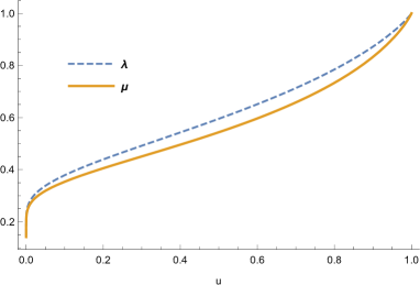
Figure 1: Plots of survival function of $X_{2:4}[Y_{2:4}]$, for all $x=-\ln u$ and $u\in(0,1]$.

The following theorem presents the usual stochastic order between the second-order statistics arising from two sets of random variables with Archimedean copula, here, we assume that the two samples have common modified proportional hazard rates parameters.

Theorem 2

Let $X_{1},X_{2}\dots,X_{n}$ be n statistically dependent heterogeneous random variables with $X_{i}\thicksim MPHR(\alpha_{i},\lambda;\overline{F};\psi)$, where $0<\alpha_{i}\leq 1,$ for all $i=1,2,\dots,n,$ and let $N_{1}$ be a non-negative integer-valued random variable independent of $X_{i}^{\prime}$s. Let $Y_{1},Y_{2}\dots,Y_{n}$ be another n statistically dependent heterogeneous random variables with $Y_{i}\thicksim MPHR(\beta_{i},\lambda;\overline{F};\psi)$, where $0<\beta_{i}\leq 1,$ for all $i=1,2,\dots,n,$ and let $N_{2}$ be another non-negative integer-valued random variable independent of $Y_{i}^{\prime}$s. Suppose $\alpha,\beta\in\mathcal{D}_{+}$ $(or\ \mathcal{I_{+}})$, if $N_{1}\geq_{\rm st}N_{2},$ and $\psi$ is log-concave. Then we have

$$\frac{1}{\alpha}\overset{\rm w}{\succeq}\frac{1}{\beta}\Rightarrow X_{2:N_{1}}\geq_{\rm st}Y_{2:N_{2}}$$

Proof 3

We present the proof for $\alpha,\beta\in\mathcal{I}_{+}$. The proof for the other case is similar, and hence not presented here. The survival function of $X_{2:n}$ can be expressed as

$$\overline{F}_{X_{2:n}}(x)=\sum\limits_{i=1}^{n}\psi\left(\sum\limits_{j\neq i}^{n}\phi\left(\frac{\alpha_{j}\overline{F}^{\lambda}(x)}{1-\overline{\alpha_{j}}\overline{F}^{\lambda}(x)}\right)\right)-(n-1)\psi\left(\sum\limits_{i=1}^{n}\phi\left(\frac{\alpha_{i}\overline{F}^{\lambda}(x)}{1-\overline{\alpha_{i}}\overline{F}^{\lambda}(x)}\right)\right).$$

Similarly, to obtain the desired result, it is then sufficient to show that $\overline{F}_{X_{2:m}}(x)\geq\overline{F}_{Y_{2:m}}(x),\ m=1,\dots,n.$ Let $a_{k}=\frac{1}{\alpha_{k}}$, for $k=1,\dots,m$. On differentiating this partially with respect to $a_{k},$ we get

$$\frac{\partial\overline{F}_{X_{2:m}}(x)}{\partial a_{k}}$$

$$= \frac{\psi\left(\phi\left(\frac{\frac{1}{a_{k}}\overline{F}^{\lambda}(x)}{1-(1-\frac{1}{a_{k}})\overline{F}^{\lambda}(x)}\right)\right)}{\psi^{\prime}\left(\phi\left(\frac{\frac{1}{a_{k}}\overline{F}^{\lambda}(x)}{1-(1-\frac{1}{a_{k}})\overline{F}^{\lambda}(x)}\right)\right)}\frac{-\frac{1}{a_{k}}[1-\overline{F}^{\lambda}(x)]}{1-(1-\frac{1}{a_{k}})\overline{F}^{\lambda}(x)}$$

$$\times\left[\sum\limits_{i\neq k}^{m}\psi^{\prime}\left(\sum\limits_{j\neq i}^{m}\phi\left(\frac{\frac{1}{a_{j}}\overline{F}^{\lambda}(x)}{1-(1-\frac{1}{a_{j}})\overline{F}^{\lambda}(x)}\right)\right)-(m-1)\psi^{\prime}\left(\sum\limits_{i=1}^{m}\phi\left(\frac{\frac{1}{a_{i}}\overline{F}^{\lambda}(x)}{1-(1-\frac{1}{a_{i}})\overline{F}^{\lambda}(x)}\right)\right)\right]$$

$$\leq 0.$$

Notice that

$$\frac{\partial\overline{F}_{X_{2:m}}(x)}{\partial a_{k}}-\frac{\partial\overline{F}_{X_{2:m}}(x)}{\partial a_{l}}$$

$$= \frac{\psi\left(\phi\left(\frac{\frac{1}{a_{k}}\overline{F}^{\lambda}(x)}{1-(1-\frac{1}{a_{k}})\overline{F}^{\lambda}(x)}\right)\right)}{\psi^{\prime}\left(\phi\left(\frac{\frac{1}{a_{k}}\overline{F}^{\lambda}(x)}{1-(1-\frac{1}{a_{k}})\overline{F}^{\lambda}(x)}\right)\right)}\frac{-\frac{1}{a_{k}}[1-\overline{F}^{\lambda}(x)]}{1-(1-\frac{1}{a_{k}})\overline{F}^{\lambda}(x)}$$

$$\times\left[\sum\limits_{i\neq k}^{m}\psi^{\prime}\left(\sum\limits_{j\neq i}^{m}\phi\left(\frac{\frac{1}{a_{j}}\overline{F}^{\lambda}(x)}{1-(1-\frac{1}{a_{j}})\overline{F}^{\lambda}(x)}\right)\right)-(m-1)\psi^{\prime}\left(\sum\limits_{i=1}^{m}\phi\left(\frac{\frac{1}{a_{i}}\overline{F}^{\lambda}(x)}{1-(1-\frac{1}{a_{i}})\overline{F}^{\lambda}(x)}\right)\right)\right]$$

$$-\frac{\psi\left(\phi\left(\frac{\frac{1}{a_{l}}\overline{F}^{\lambda}(x)}{1-(1-\frac{1}{a_{l}})\overline{F}^{\lambda}(x)}\right)\right)}{\psi^{\prime}\left(\phi\left(\frac{\frac{1}{a_{l}}\overline{F}^{\lambda}(x)}{1-(1-\frac{1}{a_{l}})\overline{F}^{\lambda}(x)}\right)\right)}\frac{-\frac{1}{a_{l}}[1-\overline{F}^{\lambda}(x)]}{1-(1-\frac{1}{a_{l}})\overline{F}^{\lambda}(x)}$$

$$\times\left[\sum\limits_{i\neq l}^{m}\psi^{\prime}\left(\sum\limits_{j\neq i}^{m}\phi\left(\frac{\frac{1}{a_{j}}\overline{F}^{\lambda}(x)}{1-(1-\frac{1}{a_{j}})\overline{F}^{\lambda}(x)}\right)\right)-(m-1)\psi^{\prime}\left(\sum\limits_{i=1}^{m}\phi\left(\frac{\frac{1}{a_{i}}\overline{F}^{\lambda}(x)}{1-(1-\frac{1}{a_{i}})\overline{F}^{\lambda}(x)}\right)\right)\right]$$

$$=: P_{2}Q_{2}-U_{2}V_{2}=P_{2}(Q_{2}-V_{2})+(P_{2}-U_{2})V_{2}.$$

For any $1\leq k<l\leq m$, $a_{k}\geq a_{l}$, by the log-concave and decreasing properties of $\psi$, we have

$$\frac{\psi\left(\phi\left(\frac{\frac{1}{a_{k}}\overline{F}^{\lambda}(x)}{1-(1-\frac{1}{a_{k}})\overline{F}^{\lambda}(x)}\right)\right)}{\psi^{\prime}\left(\phi\left(\frac{\frac{1}{a_{k}}\overline{F}^{\lambda}(x)}{1-(1-\frac{1}{a_{k}})\overline{F}^{\lambda}(x)}\right)\right)}\geq\frac{\psi\left(\phi\left(\frac{\frac{1}{a_{l}}\overline{F}^{\lambda}(x)}{1-(1-\frac{1}{a_{l}})\overline{F}^{\lambda}(x)}\right)\right)}{\psi^{\prime}\left(\phi\left(\frac{\frac{1}{a_{l}}\overline{F}^{\lambda}(x)}{1-(1-\frac{1}{a_{l}})\overline{F}^{\lambda}(x)}\right)\right)}.$$

It holds that

$$(P_{2}-U_{2})V_{2}$$

$$\overset{\rm sgn}{=} \frac{\psi\left(\phi\left(\frac{\frac{1}{a_{k}}\overline{F}^{\lambda}(x)}{1-(1-\frac{1}{a_{k}})\overline{F}^{\lambda}(x)}\right)\right)}{\psi^{\prime}\left(\phi\left(\frac{\frac{1}{a_{k}}\overline{F}^{\lambda}(x)}{1-(1-\frac{1}{a_{k}})\overline{F}^{\lambda}(x)}\right)\right)}\frac{\frac{1}{a_{k}}}{1-(1-\frac{1}{a_{k}})\overline{F}^{\lambda}(x)}-\frac{\psi\left(\phi\left(\frac{\frac{1}{a_{l}}\overline{F}^{\lambda}(x)}{1-(1-\frac{1}{a_{l}})\overline{F}^{\lambda}(x)}\right)\right)}{\psi^{\prime}\left(\phi\left(\frac{\frac{1}{a_{l}}\overline{F}^{\lambda}(x)}{1-(1-\frac{1}{a_{l}})\overline{F}^{\lambda}(x)}\right)\right)}\frac{\frac{1}{a_{l}}}{1-(1-\frac{1}{a_{l}})\overline{F}^{\lambda}(x)}$$

$$= \frac{\psi\left(\phi\left(\frac{\frac{1}{a_{k}}\overline{F}^{\lambda}(x)}{1-(1-\frac{1}{a_{k}})\overline{F}^{\lambda}(x)}\right)\right)}{\psi^{\prime}\left(\phi\left(\frac{\frac{1}{a_{k}}\overline{F}^{\lambda}(x)}{1-(1-\frac{1}{a_{k}})\overline{F}^{\lambda}(x)}\right)\right)}\left[\frac{\frac{1}{a_{k}}}{1-(1-\frac{1}{a_{k}})\overline{F}^{\lambda}(x)}-\frac{\frac{1}{a_{l}}}{1-(1-\frac{1}{a_{l}})\overline{F}^{\lambda}(x)}\right]$$

$$+\frac{\frac{1}{a_{l}}}{1-(1-\frac{1}{a_{l}})\overline{F}^{\lambda}(x)}\left[\frac{\psi\left(\phi\left(\frac{\frac{1}{a_{k}}\overline{F}^{\lambda}(x)}{1-(1-\frac{1}{a_{k}})\overline{F}^{\lambda}(x)}\right)\right)}{\psi^{\prime}\left(\phi\left(\frac{\frac{1}{a_{k}}\overline{F}^{\lambda}(x)}{1-(1-\frac{1}{a_{k}})\overline{F}^{\lambda}(x)}\right)\right)}-\frac{\psi\left(\phi\left(\frac{\frac{1}{a_{l}}\overline{F}^{\lambda}(x)}{1-(1-\frac{1}{a_{l}})\overline{F}^{\lambda}(x)}\right)\right)}{\psi^{\prime}\left(\phi\left(\frac{\frac{1}{a_{l}}\overline{F}^{\lambda}(x)}{1-(1-\frac{1}{a_{l}})\overline{F}^{\lambda}(x)}\right)\right)}\right]$$

$$\geq 0.$$

For any $a_{k}\geq a_{l}$, owing to $\phi$ is convex and decreasing, we have

$$\psi^{\prime}\left(\sum\limits_{j\neq k}^{m}\phi\left(\frac{\frac{1}{a_{j}}\overline{F}^{\lambda}(x)}{1-(1-\frac{1}{a_{j}})\overline{F}^{\lambda}(x)}\right)\right)\leq\psi^{\prime}\left(\sum\limits_{j\neq l}^{m}\phi\left(\frac{\frac{1}{a_{j}}\overline{F}^{\lambda}(x)}{1-(1-\frac{1}{a_{j}})\overline{F}^{\lambda}(x)}\right)\right).$$

As a result, we have

$$P_{2}(Q_{2}-V_{2}) \overset{\rm sgn}{=} \sum\limits_{i\neq k}^{m}\psi^{\prime}\left(\sum\limits_{j\neq i}^{m}\phi\left(\frac{\frac{1}{a_{j}}\overline{F}^{\lambda}(x)}{1-(1-\frac{1}{a_{j}})\overline{F}^{\lambda}(x)}\right)\right)-\sum\limits_{i\neq l}^{m}\psi^{\prime}\left(\sum\limits_{j\neq i}^{m}\phi\left(\frac{\frac{1}{a_{j}}\overline{F}^{\lambda}(x)}{1-(1-\frac{1}{a_{j}})\overline{F}^{\lambda}(x)}\right)\right)$$

$$= \psi^{\prime}\left(\sum\limits_{j\neq l}^{m}\phi\left(\frac{\frac{1}{a_{j}}\overline{F}^{\lambda}(x)}{1-(1-\frac{1}{a_{j}})\overline{F}^{\lambda}(x)}\right)\right)-\psi^{\prime}\left(\sum\limits_{j\neq k}^{m}\phi\left(\frac{\frac{1}{a_{j}}\overline{F}^{\lambda}(x)}{1-(1-\frac{1}{a_{j}})\overline{F}^{\lambda}(x)}\right)\right)$$

$$\geq 0.$$

Therefore, the desires result completed by lemma 1.

Remark 2

The result of Theorem 2 improves Theorem 2 of Zhang et al. (2021) from the extreme order statistics to the case of the second-order statistics.

The next example illustrates result of Theorem 2.

Example 2

Consider the case of $n=4$. Let $\overline{F}(x)=e^{-(ax)^{b}},a>0,b>0$, and generator $\psi(x)=e^{1-(1+x)^{\theta}},\theta>0.$ Taking $\lambda=0.4,a=0,5,b=0.8,\theta=7,\alpha=(\frac{1}{3},\frac{1}{3},\frac{1}{5},\frac{1}{8})\ and\ \beta=(\frac{1}{5},\frac{1}{6},\frac{1}{7},\frac{1}{9}).$ Evidently, $(\frac{1}{\alpha_{1}},\frac{1}{\alpha_{2}},\frac{1}{\alpha_{3}},\frac{1}{\alpha_{4}})\overset{\rm w}{\succeq}(\frac{1}{\beta_{1}},\frac{1}{\beta_{2}},\frac{1}{\beta_{3}},\frac{1}{\beta_{4}}).$ Let $N_{1}$ be an integer-valued random variable having the probability distribution $\mathbb{P}(N_{1}=1)=0.05,\mathbb{P}(N_{1}=2)=0.2,\mathbb{P}(N_{1}=3)=0.3,\mathbb{P}(N_{1}=4)=0.45$, and $N_{2}$ be another integer-valued random variable with the probability distribution $\mathbb{P}(N_{2}=1)=0.05,\mathbb{P}(N_{2}=2)=0.2,\mathbb{P}(N_{2}=3)=0.35,\mathbb{P}(N_{2}=4)=0.4$, it is apparently that $N_{1}\geq_{\rm st}N_{2}$. The plots of survival functions of $X_{2:4}$ and $Y_{2:4}$, denoted as $\overline{F}_{X_{2:4}}$ and $\overline{F}_{Y_{2:4}}$, are plotted in figure 2, all $x=-{\rm ln}(u)$ and $u\in(0,1]$. Thus, the effectiveness of Theorem 1 are vaidated.

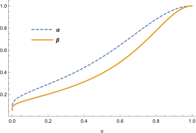
Figure 2: Plots of survival function of $X_{2:4}[Y_{2:4}]$, for all $x=-\ln u$ and $u\in(0,1]$.

4 Hazard rate order of second-order statistics from independent and heterogeneous observations

The next theorem gives sufficient conditions guaranteeing the hazard rate order between two modified proportional hazard rates models with the same modified proportional hazard rates parameters and the heterogeneous tilt parameters.

Theorem 3

Let $X_{1},X_{2}\dots,X_{n}$ be n independent heterogeneous random variables with $X_{i}\thicksim MPHR(\alpha_{i},\lambda;\overline{F})$, where $0<\alpha_{i}\leq 1,$ for all $i=1,2,\dots,n.$ Let $Y_{1},Y_{2}\dots,Y_{n}$ be another n independent heterogeneous random variables with $Y_{i}\thicksim MPHR(\beta_{i},\lambda;\overline{F})$, where $0<\beta_{i}\leq 1,$ for all $i=1,2,\dots,n$. Suppose $\alpha,\beta\in\mathcal{D}_{+}$ $(or\ \mathcal{I_{+}})$. Then we have

$$\frac{1}{\alpha}\overset{\rm m}{\succeq}\frac{1}{\beta}\Rightarrow X_{2:n}\geq_{\rm hr}Y_{2:n}.$$

Proof 4

The idea of the proof is borrowed from Theorem 3.7 of Das & Kayal (2021a). The survival function of $X_{2:n}$ can be rewritten

$$\overline{F}_{X_{2:n}}(x) = \sum\limits^{n}_{i=1}\prod\limits^{n}_{j\neq i}\frac{\alpha_{j}\overline{F}^{\lambda}(x)}{1-\overline{\alpha_{j}}\overline{F}^{\lambda}(x)}-(n-1)\prod\limits^{n}_{i=1}\frac{\alpha_{i}\overline{F}^{\lambda}(x)}{1-\overline{\alpha_{i}}\overline{F}^{\lambda}(x)}$$

$$= \prod\limits^{n}_{i=1}\frac{\alpha_{i}\overline{F}^{\lambda}(x)}{1-\overline{\alpha_{i}}\overline{F}^{\lambda}(x)}\left[\sum\limits^{n}_{i=1}\frac{1-\overline{\alpha_{i}}\overline{F}^{\lambda}(x)}{\alpha_{i}\overline{F}^{\lambda}(x)}-(n-1)\right]$$

$$= \prod\limits^{n}_{i=1}\frac{\alpha_{i}\overline{F}^{\lambda}(x)}{1-\overline{\alpha_{i}}\overline{F}^{\lambda}(x)}\left[\sum\limits^{n}_{i=1}\frac{1-\overline{F}^{\lambda}(x)}{\alpha_{i}\overline{F}^{\lambda}(x)}+1\right].$$

Thus, the hazard rate function of the second-order statistic $X_{2:n}$ can be obtained as

$$r_{X_{2:n}}(x)=\sum\limits^{n}_{i=1}\frac{\lambda r(x)}{1-\overline{\alpha}_{i}\overline{F}^{\lambda}(x)}-\frac{\sum\limits^{n}_{i=1}\frac{\lambda r(x)}{\alpha_{i}\overline{F}^{\lambda}(x)}}{\sum\limits^{n}_{i=1}\frac{1-\overline{F}^{\lambda}(x)}{\alpha_{i}\overline{F}^{\lambda}(x)}+1},$$

where $r(x)$ is the hazard rate function of the baseline distribution. Define

$$\Phi(a)=r_{X_{2:n}}(x)=\sum\limits^{n}_{i=1}\frac{\lambda r(x)}{1-(1-\frac{1}{a_{i}})\overline{F}^{\lambda}(x)}-\frac{\sum\limits^{n}_{i=1}\frac{a_{i}\lambda r(x)}{\overline{F}^{\lambda}(x)}}{\sum\limits^{n}_{i=1}\frac{a_{i}(1-\overline{F}^{\lambda}(x))}{\overline{F}^{\lambda}(x)}+1},$$ (5)

where $a_{i}=\frac{1}{\alpha_{i}}$, $i=1,\dots,n.$ After differentiating equation (5) partially with respect to $a_{k},$ we obtain

$$\frac{\partial\Phi(a)}{\partial a_{k}}=\frac{\frac{1}{a^{2}_{k}}\overline{F}^{\lambda}(x)\lambda r(x)}{\left[1-(1-\frac{1}{a_{k}})\overline{F}^{\lambda}(x)\right]^{2}}-\frac{\frac{\lambda r(x)}{\overline{F}^{\lambda}(x)}}{\sum\limits^{n}_{i=1}\frac{a_{i}(1-\overline{F}^{\lambda}(x))}{\overline{F}^{\lambda}(x)}+1}+\frac{\sum\limits^{n}_{i=1}\frac{a_{i}\lambda r(x)}{\overline{F}^{\lambda}(x)}\frac{1-\overline{F}^{\lambda}(x)}{\overline{F}^{\lambda}(x)}}{\left[\sum\limits^{n}_{i=1}\frac{a_{i}(1-\overline{F}^{\lambda}(x))}{\overline{F}^{\lambda}(x)}+1\right]^{2}}.$$ (6)

To prove the result, it is sufficient to show that $\Phi(a)$ is schur-concave with respect to $a\in\mathcal{I_{+}}$ $or\mathcal{D_{+}}$. Without loss of generality, let $a\in\mathcal{I_{+}}$, for any $1\leq k<l\leq n,$ $a_{k}\leq a_{l}$. Using (6), we have

$$\frac{\partial\Phi(a)}{\partial a_{k}}-\frac{\partial\Phi(a)}{\partial a_{l}} \overset{\rm sgn}{=} \frac{\frac{1}{a^{2}_{k}}}{\left[1-(1-\frac{1}{a_{k}})\overline{F}^{\lambda}(x)\right]^{2}}-\frac{\frac{1}{a^{2}_{l}}}{\left[1-(1-\frac{1}{a_{l}})\overline{F}^{\lambda}(x)\right]^{2}}\geq 0,$$

where the last inequality is due to lemma 3. Thus, the result follows from Lemma 2.

The following example illustrates the result of Theorem 3.

Remark 3

The result of Theorem 3 completes Theorem 3 of Zhang et al. (2021) from the extreme order statistics to the case of the second-order statistics.

Example 3

Let $\overline{F}(x)=e^{-(ax)^{b}},a>0,b>0$, Set $n=4,\lambda=0.5,a=0.15,b=1.2,\alpha=(\frac{1}{4},\frac{1}{3},\frac{1}{2},1)\ and\ \beta=(\frac{1}{3},\frac{1}{3},\frac{1}{2},\frac{1}{2}).$ Evidently, $(\frac{1}{\alpha_{1}},\frac{1}{\alpha_{2}},\frac{1}{\alpha_{3}},\frac{1}{\alpha_{4}})\overset{\rm m}{\succeq}(\frac{1}{\beta_{1}},\frac{1}{\beta_{2}},\frac{1}{\beta_{3}},\frac{1}{\beta_{4}}).$ One can verify that the conditions of Theorem 3 are all statisfied. Figure 3 plots the hazard rate functions of $X_{2:4}$ and $Y_{2:4}$, denoted as $r_{X_{2:4}}(x)$ and $r_{Y_{2:4}}(x)$, all $x=-{\rm ln}(u)$ and $u\in(0,1]$. Thus, we can get $X_{2:4}\geq_{\rm hr}Y_{2:4}$.

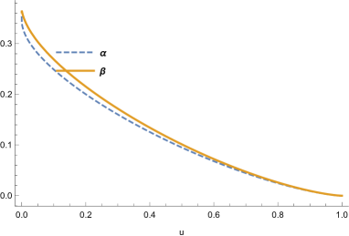
Figure 3: Plots of hazard rate functions of $X_{2:4}[Y_{2:4}]$, for all $x=-\ln u$ and $u\in(0,1]$.

In the next, we discuss stochastic comparisons on the second-order statistics arising from multiple-outlier MPHR samples in the sense of the hazard rate order. We first present the following result.

Theorem 4

Let $X_{1},X_{2},\dots,X_{n}$ be independent random variables following the multiple-outlier MPHR moder with survival functions$(\frac{\alpha\overline{F}^{\lambda_{1}}(x)}{1-\overline{\alpha}\overline{F}^{\lambda_{1}}(x)}{\rm I}_{p},\frac{\alpha\overline{F}^{\lambda}(x)}{1-\overline{\alpha}\overline{F}^{\lambda}(x)}{\rm I}_{q}),$ where $p+q=n,p,q\geq 1,$ $\overline{F}(x)$ is the baseline survival function, and ${\rm I}_{p}$ stand for a p-dimensional vector with all its components equal to 1.Let $Y_{1},Y_{2},\dots,Y_{n}$ be another set of independent random variables following the multiple-outlier MPHR moder with survival functions$(\frac{\alpha\overline{F}^{\lambda_{2}}(x)}{1-\overline{\alpha}\overline{F}^{\lambda_{2}}(x)}{\rm I}_{p},\frac{\alpha\overline{F}^{\lambda}(x)}{1-\overline{\alpha}\overline{F}^{\lambda}(x)}{\rm I}_{q}).$ If $\lambda\geq\lambda_{2}\geq\lambda_{1},$ then $X_{2:n}\geq_{\rm hr}Y_{2:n}.$

Proof 5

The idea of the proof is borrowed from Theorem 3.1 of Cai et al. (2017). The survival function of $X_{2:n}$ and $Y_{2:n}$ are given by

$$\overline{F}_{X_{2:n}}(x) = p\left[\frac{\alpha\overline{F}^{\lambda_{1}}(x)}{1-\overline{\alpha}\overline{F}^{\lambda_{1}}(x)}\right]^{p-1}\left[\frac{\alpha\overline{F}^{\lambda}(x)}{1-\overline{\alpha}\overline{F}^{\lambda}(x)}\right]^{q}+q\left[\frac{\alpha\overline{F}^{\lambda_{1}}(x)}{1-\overline{\alpha}\overline{F}^{\lambda_{1}}(x)}\right]^{p}\left[\frac{\alpha\overline{F}^{\lambda}(x)}{1-\overline{\alpha}\overline{F}^{\lambda}(x)}\right]^{q-1}$$

$$-(n-1)\left[\frac{\alpha\overline{F}^{\lambda_{1}}(x)}{1-\overline{\alpha}\overline{F}^{\lambda_{1}}(x)}\right]^{p}\left[\frac{\alpha\overline{F}^{\lambda}(x)}{1-\overline{\alpha}\overline{F}^{\lambda}(x)}\right]^{q},$$

and

$$\overline{F}_{X^{*}_{2:n}}(x) = p\left[\frac{\alpha\overline{F}^{\lambda_{2}}(x)}{1-\overline{\alpha}\overline{F}^{\lambda_{2}}(x)}\right]^{p-1}\left[\frac{\alpha\overline{F}^{\lambda}(x)}{1-\overline{\alpha}\overline{F}^{\lambda}(x)}\right]^{q}+q\left[\frac{\alpha\overline{F}^{\lambda_{2}}(x)}{1-\overline{\alpha}\overline{F}^{\lambda_{2}}(x)}\right]^{p}\left[\frac{\alpha\overline{F}^{\lambda}(x)}{1-\overline{\alpha}\overline{F}^{\lambda}(x)}\right]^{q-1}$$

$$-(n-1)\left[\frac{\alpha\overline{F}^{\lambda_{2}}(x)}{1-\overline{\alpha}\overline{F}^{\lambda_{2}}(x)}\right]^{p}\left[\frac{\alpha\overline{F}^{\lambda}(x)}{1-\overline{\alpha}\overline{F}^{\lambda}(x)}\right]^{q},$$

where $\overline{\alpha}=1-\alpha$ and $p+q=n.$ Let us set $\overline{F}^{\lambda}(x)=e^{-\lambda(-{\rm ln}\overline{F}(x))}$ and $t=-{\rm ln}\overline{F}(x)$. We can then rewritten the survival function $X_{2:n}$ as:

$$\overline{F}_{X_{2:n}}(t) = p\left[\frac{\alpha}{e^{\lambda_{1}t}-\overline{\alpha}}\right]^{p-1}\left[\frac{\alpha}{e^{\lambda t}-\overline{\alpha}}\right]^{q}+q\left[\frac{\alpha}{e^{\lambda_{1}t}-\overline{\alpha}}\right]^{p}\left[\frac{\alpha}{e^{\lambda t}-\overline{\alpha}}\right]^{q-1}$$

$$-(n-1)\left[\frac{\alpha}{e^{\lambda_{1}t}-\overline{\alpha}}\right]^{p}\left[\frac{\alpha}{e^{\lambda t}-\overline{\alpha}}\right]^{q},t\geq 0.$$

Thus, its hazard rate function is given by

$$r_{X_{2:n}}(t) = \frac{{\rm d}[-{\rm ln}\overline{F}_{X_{2:n}}(t)]}{{\rm d}t}=\frac{pA_{1}\left(\frac{e^{\lambda_{1}t}-\overline{\alpha}}{\alpha}\right)+qA_{2}\left(\frac{e^{\lambda t}-\overline{\alpha}}{\alpha}\right)-(n-1)A}{p\left(\frac{e^{\lambda_{1}t}-\overline{\alpha}}{\alpha}\right)+q\left(\frac{e^{\lambda t}-\overline{\alpha}}{\alpha}\right)-(n-1)},$$

where $A_{1}=(p-1)\frac{\lambda_{1}e^{\lambda_{1}t}}{e^{\lambda_{1}t}-\overline{\alpha}}+q\frac{\lambda e^{\lambda t}}{e^{\lambda t}-\overline{\alpha}}$, $A_{2}=p\frac{\lambda_{1}e^{\lambda_{1}t}}{e^{\lambda_{1}t}-\overline{\alpha}}+(q-1)\frac{\lambda e^{\lambda t}}{e^{\lambda t}-\overline{\alpha}}$ and $A=p\frac{\lambda_{1}e^{\lambda_{1}t}}{e^{\lambda_{1}t}-\overline{\alpha}}+q\frac{\lambda e^{\lambda t}}{e^{\lambda t}-\overline{\alpha}}$. It suffices to show $r_{X_{2:n}}(t)\leq r_{X^{*}_{2:n}}(t)$ for $\lambda\geq\lambda_{2}\geq\lambda_{1}>0,$ i.e.,

$$\frac{pA_{1}\left(\frac{e^{\lambda_{1}t}-\overline{\alpha}}{\alpha}\right)+qA_{2}\left(\frac{e^{\lambda t}-\overline{\alpha}}{\alpha}\right)-(n-1)A}{p\left(\frac{e^{\lambda_{1}t}-\overline{\alpha}}{\alpha}\right)+q\left(\frac{e^{\lambda t}-\overline{\alpha}}{\alpha}\right)-(n-1)}\leq\frac{pB_{1}\left(\frac{e^{\lambda_{2}t}-\overline{\alpha}}{\alpha}\right)+qB_{2}\left(\frac{e^{\lambda t}-\overline{\alpha}}{\alpha}\right)-(n-1)B}{p\left(\frac{e^{\lambda_{2}t}-\overline{\alpha}}{\alpha}\right)+q\left(\frac{e^{\lambda t}-\overline{\alpha}}{\alpha}\right)-(n-1)}.$$

where $B_{1}=(p-1)\frac{\lambda_{2}e^{\lambda_{2}t}}{e^{\lambda_{2}t}-\overline{\alpha}}+q\frac{\lambda e^{\lambda t}}{e^{\lambda t}-\overline{\alpha}}$, $B_{2}=p\frac{\lambda_{2}e^{\lambda_{2}t}}{e^{\lambda_{2}t}-\overline{\alpha}}+(q-1)\frac{\lambda e^{\lambda t}}{e^{\lambda t}-\overline{\alpha}}$ and $B=p\frac{\lambda_{2}e^{\lambda_{2}t}}{e^{\lambda_{2}t}-\overline{\alpha}}+q\frac{\lambda e^{\lambda t}}{e^{\lambda t}-\overline{\alpha}}$, or equivalently

$$\Bigg{\{}p\left[(p-1)\frac{\lambda_{1}e^{\lambda_{1}t}}{e^{\lambda_{1}t}-\overline{\alpha}}+q\frac{\lambda e^{\lambda t}}{e^{\lambda t}-\overline{\alpha}}\right]\left(\frac{e^{\lambda_{1}t}-\overline{\alpha}}{\alpha}\right)+q\left[p\frac{\lambda_{1}e^{\lambda_{1}t}}{e^{\lambda_{1}t}-\overline{\alpha}}+(q-1)\frac{\lambda e^{\lambda t}}{e^{\lambda t}-\overline{\alpha}}\right]\left(\frac{e^{\lambda t}-\overline{\alpha}}{\alpha}\right)$$

$$-(n-1)\left[p\frac{\lambda_{1}e^{\lambda_{1}t}}{e^{\lambda_{1}t}-\overline{\alpha}}+q\frac{\lambda e^{\lambda t}}{e^{\lambda t}-\overline{\alpha}}\right]\Bigg{\}}\times\frac{1}{p\left(\frac{e^{\lambda_{1}t}-\overline{\alpha}}{\alpha}\right)+q\left(\frac{e^{\lambda t}-\overline{\alpha}}{\alpha}\right)-(n-1)}$$

$$\leq \Bigg{\{}p\left[(p-1)\frac{\lambda_{2}e^{\lambda_{2}t}}{e^{\lambda_{2}t}-\overline{\alpha}}+q\frac{\lambda e^{\lambda t}}{e^{\lambda t}-\overline{\alpha}}\right]\left(\frac{e^{\lambda_{2}t}-\overline{\alpha}}{\alpha}\right)+q\left[p\frac{\lambda_{2}e^{\lambda_{2}t}}{e^{\lambda_{2}t}-\overline{\alpha}}+(q-1)\frac{\lambda e^{\lambda t}}{e^{\lambda t}-\overline{\alpha}}\right]\left(\frac{e^{\lambda t}-\overline{\alpha}}{\alpha}\right)$$

$$-(n-1)\left[p\frac{\lambda_{2}e^{\lambda_{2}t}}{e^{\lambda_{2}t}-\overline{\alpha}}+q\frac{\lambda e^{\lambda t}}{e^{\lambda t}-\overline{\alpha}}\right]\Bigg{\}}\times\frac{1}{p\left(\frac{e^{\lambda_{2}t}-\overline{\alpha}}{\alpha}\right)+q\left(\frac{e^{\lambda t}-\overline{\alpha}}{\alpha}\right)-(n-1)}.$$

Denote by

$$M_{1} = \frac{1}{p\left(\frac{e^{\lambda_{1}t}-\overline{\alpha}}{\alpha}\right)+q\left(\frac{e^{\lambda t}-\overline{\alpha}}{\alpha}\right)-(n-1)}\times\Bigg{\{}p\left[(p-1)\frac{\lambda_{1}e^{\lambda_{1}t}}{e^{\lambda_{1}t}-\overline{\alpha}}+q\frac{\lambda e^{\lambda t}}{e^{\lambda t}-\overline{\alpha}}\right]\left(\frac{e^{\lambda_{1}t}-\overline{\alpha}}{\alpha}\right)$$

$$+q\left[p\frac{\lambda_{1}e^{\lambda_{1}t}}{e^{\lambda_{1}t}-\overline{\alpha}}+(q-1)\frac{\lambda e^{\lambda t}}{e^{\lambda t}-\overline{\alpha}}\right]\left(\frac{e^{\lambda t}-\overline{\alpha}}{\alpha}\right)-(n-1)\left[p\frac{\lambda_{1}e^{\lambda_{1}t}}{e^{\lambda_{1}t}-\overline{\alpha}}+q\frac{\lambda e^{\lambda t}}{e^{\lambda t}-\overline{\alpha}}\right]\Bigg{\}},$$

$$M_{2} = \frac{1}{p\left(\frac{e^{\lambda_{2}t}-\overline{\alpha}}{\alpha}\right)+q\left(\frac{e^{\lambda t}-\overline{\alpha}}{\alpha}\right)-(n-1)}\times\Bigg{\{}p\left[(p-1)\frac{\lambda_{1}e^{\lambda_{1}t}}{e^{\lambda_{1}t}-\overline{\alpha}}+q\frac{\lambda e^{\lambda t}}{e^{\lambda t}-\overline{\alpha}}\right]\left(\frac{e^{\lambda_{2}t}-\overline{\alpha}}{\alpha}\right)$$

$$+q\left[p\frac{\lambda_{1}e^{\lambda_{1}t}}{e^{\lambda_{1}t}-\overline{\alpha}}+(q-1)\frac{\lambda e^{\lambda t}}{e^{\lambda t}-\overline{\alpha}}\right]\left(\frac{e^{\lambda t}-\overline{\alpha}}{\alpha}\right)-(n-1)\left[p\frac{\lambda_{1}e^{\lambda_{1}t}}{e^{\lambda_{1}t}-\overline{\alpha}}+q\frac{\lambda e^{\lambda t}}{e^{\lambda t}-\overline{\alpha}}\right]\Bigg{\}},$$

$$M_{3} = \frac{1}{p\left(\frac{e^{\lambda_{2}t}-\overline{\alpha}}{\alpha}\right)+q\left(\frac{e^{\lambda t}-\overline{\alpha}}{\alpha}\right)-(n-1)}\times\Bigg{\{}p\left[(p-1)\frac{\lambda_{2}e^{\lambda_{2}t}}{e^{\lambda_{2}t}-\overline{\alpha}}+q\frac{\lambda e^{\lambda t}}{e^{\lambda t}-\overline{\alpha}}\right]\left(\frac{e^{\lambda_{2}t}-\overline{\alpha}}{\alpha}\right)$$

$$+q\left[p\frac{\lambda_{2}e^{\lambda_{2}t}}{e^{\lambda_{2}t}-\overline{\alpha}}+(q-1)\frac{\lambda e^{\lambda t}}{e^{\lambda t}-\overline{\alpha}}\right]\left(\frac{e^{\lambda t}-\overline{\alpha}}{\alpha}\right)-(n-1)\left[p\frac{\lambda_{2}e^{\lambda_{2}t}}{e^{\lambda_{2}t}-\overline{\alpha}}+q\frac{\lambda e^{\lambda t}}{e^{\lambda t}-\overline{\alpha}}\right]\Bigg{\}}.$$

For $\lambda\geq\lambda_{2}\geq\lambda_{1}>0$, by the increasing properties of $\frac{\lambda e^{\lambda t}}{e^{\lambda t}-\overline{\alpha}}$ with respect to $\lambda$, we have

$$\frac{\lambda_{2}e^{\lambda_{2}t}}{e^{\lambda_{2}t}-\overline{\alpha}}\geq\frac{\lambda_{1}e^{\lambda_{1}t}}{e^{\lambda_{1}t}-\overline{\alpha}}.$$

It holds that

$$M_{3}-M_{2} \overset{\rm sgn}{=} p(p-1)\left(\frac{e^{\lambda_{2}t}-\overline{\alpha}}{\alpha}\right)\left[\frac{\lambda_{2}e^{\lambda_{2}t}}{e^{\lambda_{2}t}-\overline{\alpha}}-\frac{\lambda_{1}e^{\lambda_{1}t}}{e^{\lambda_{1}t}-\overline{\alpha}}\right]+pq\left(\frac{e^{\lambda t}-\overline{\alpha}}{\alpha}\right)\times\left[\frac{\lambda_{2}e^{\lambda_{2}t}}{e^{\lambda_{2}t}-\overline{\alpha}}-\frac{\lambda_{1}e^{\lambda_{1}t}}{e^{\lambda_{1}t}-\overline{\alpha}}\right]$$

$$-p(n-1)\left[\frac{\lambda_{2}e^{\lambda_{2}t}}{e^{\lambda_{2}t}-\overline{\alpha}}-\frac{\lambda_{1}e^{\lambda_{1}t}}{e^{\lambda_{1}t}-\overline{\alpha}}\right]$$

$$= p\left[\frac{\lambda_{2}e^{\lambda_{2}t}}{e^{\lambda_{2}t}-\overline{\alpha}}-\frac{\lambda_{1}e^{\lambda_{1}t}}{e^{\lambda_{1}t}-\overline{\alpha}}\right]\left[(p-1)\left(\frac{e^{\lambda_{2}t}-\overline{\alpha}}{\alpha}\right)+q\left(\frac{e^{\lambda t}-\overline{\alpha}}{\alpha}\right)-(n-1)\right]$$

$$\geq p\left[\frac{\lambda_{2}e^{\lambda_{2}t}}{e^{\lambda_{2}t}-\overline{\alpha}}-\frac{\lambda_{1}e^{\lambda_{1}t}}{e^{\lambda_{1}t}-\overline{\alpha}}\right]\left[p+q-1-(n-1)\right]$$

$$= 0.$$

Which implies that $M_{2}\leq M_{3}$. Let

$$P=q\left[p\frac{\lambda_{1}e^{\lambda_{1}t}}{e^{\lambda_{1}t}-\overline{\alpha}}+(q-1)\frac{\lambda e^{\lambda t}}{e^{\lambda t}-\overline{\alpha}}\right]\left(\frac{e^{\lambda t}-\overline{\alpha}}{\alpha}\right)-(n-1)\left[p\frac{\lambda_{1}e^{\lambda_{1}t}}{e^{\lambda_{1}t}-\overline{\alpha}}+q\frac{\lambda e^{\lambda t}}{e^{\lambda t}-\overline{\alpha}}\right]$$

$$Q=p\left[(p-1)\frac{\lambda_{1}e^{\lambda_{1}t}}{e^{\lambda_{1}t}-\overline{\alpha}}+q\frac{\lambda e^{\lambda t}}{e^{\lambda t}-\overline{\alpha}}\right]$$

$$U=q\left(\frac{e^{\lambda t}-\overline{\alpha}}{\alpha}\right)-(n-1)\quad and\quad V=p.$$

So, we have

$$QU-PV = pq\left(\frac{e^{\lambda t}-\overline{\alpha}}{\alpha}\right)\left[\frac{\lambda e^{\lambda t}}{e^{\lambda t}-\overline{\alpha}}-\frac{\lambda_{1}e^{\lambda_{1}t}}{e^{\lambda_{1}t}-\overline{\alpha}}\right]+p(n-1)\left(\frac{\lambda_{1}e^{\lambda_{1}t}}{e^{\lambda_{1}t}-\overline{\alpha}}\right)\geq 0.$$

So,we have

$$M_{2}-M_{1} = \frac{Q\left(\frac{e^{\lambda_{2}t}-\overline{\alpha}}{\alpha}\right)+P}{V\left(\frac{e^{\lambda_{2}t}-\overline{\alpha}}{\alpha}\right)+U}-\frac{Q\left(\frac{e^{\lambda_{1}t}-\overline{\alpha}}{\alpha}\right)+P}{V\left(\frac{e^{\lambda_{1}t}-\overline{\alpha}}{\alpha}\right)+U}$$

$$= \frac{\left[Q\left(\frac{e^{\lambda_{2}t}-\overline{\alpha}}{\alpha}\right)+P\right]\left[V\left(\frac{e^{\lambda_{1}t}-\overline{\alpha}}{\alpha}\right)+U\right]-\left[Q\left(\frac{e^{\lambda_{1}t}-\overline{\alpha}}{\alpha}\right)+P\right]\left[V\left(\frac{e^{\lambda_{2}t}-\overline{\alpha}}{\alpha}\right)+U\right]}{\left[V\left(\frac{e^{\lambda_{2}t}-\overline{\alpha}}{\alpha}\right)+U\right]\left[V\left(\frac{e^{\lambda_{1}t}-\overline{\alpha}}{\alpha}\right)+U\right]}$$

$$\overset{\rm sgn}{=} (QU-PV)\left(\frac{e^{\lambda_{2}t}-\overline{\alpha}}{\alpha}-\frac{e^{\lambda_{1}t}-\overline{\alpha}}{\alpha}\right)$$

$$\geq 0,$$

which means that $M_{1}\leq M_{2}$. Thus, $M_{1}\leq M_{3}$, and the theorem follows.

In the next, we turn to discuss the effect generated by the discrepancy among sample sizes on the hazard rate function of the second-order statistic arising from multiple-outlier MPHR samples.

Theorem 5

Let $X_{1},X_{2},\dots,X_{p},X_{p+1},\dots,X_{n}$ be independentrandom variables following the multiple-outlier MPHR moder with survival functions$(\frac{\alpha\overline{F}^{\lambda_{1}}(x)}{1-\overline{\alpha}\overline{F}^{\lambda_{1}}(x)}{\rm I}_{p},\frac{\alpha\overline{F}^{\lambda_{2}}(x)}{1-\overline{\alpha}\overline{F}^{\lambda_{2}}(x)}{\rm I}_{q}),$ where $p+q=n,p,q\geq 1$ and $\overline{F}(x)$ is the baseline survival function.Let $Y_{1},Y_{2},\dots,Y_{p^{*}},Y_{p^{*}+1},\dots,Y_{n^{*}}$ be another set of independent random variables following the multiple-outlier MPHR moder with survival functions$(\frac{\alpha\overline{F}^{\lambda_{1}}(x)}{1-\overline{\alpha}\overline{F}^{\lambda_{1}}(x)}{\rm I}_{p}^{*},\frac{\alpha\overline{F}^{\lambda_{2}}(x)}{1-\overline{\alpha}\overline{F}^{\lambda_{2}}(x)}{\rm I}_{q}^{*}),$ where $p^{*}+q^{*}=n^{*},p^{*},q^{*}\geq 1$. Denote by $X_{2:n}$ and $Y_{2:n^{*}}$ the second-order statistic arising from these two sets of multiple-outlier MPHR models, respectively. Suppose that $p^{*}\leq p\leq q\leq q^{*}$ and $\lambda_{1}\leq\lambda_{2}$.Then, we have

$$(p,q)\preceq_{\rm w}(p^{*},q^{*})\Rightarrow X_{2:n}\geq_{\rm hr}Y_{2:n^{*}}$$

Proof 6

The idea of the proof is borrowed from Theorem 3.4 of Cai et al. (2017). Following the notation in the proof of Theorem 4, the hazard rate function of $X_{2:n}$ can be written as follows:

$$r_{X_{2:n}}(t)=\frac{pT_{1}\left(\frac{e^{\lambda_{1}t}-\overline{\alpha}}{\alpha}\right)+qT_{2}\left(\frac{e^{\lambda_{2}t}-\overline{\alpha}}{\alpha}\right)-(n-1)T}{p\left(\frac{e^{\lambda_{1}t}-\overline{\alpha}}{\alpha}\right)+q\left(\frac{e^{\lambda_{2}t}-\overline{\alpha}}{\alpha}\right)-(n-1)},$$

where $T_{1}=(p-1)\frac{\lambda_{1}e^{\lambda_{1}t}}{e^{\lambda_{1}t}-\overline{\alpha}}+q\frac{\lambda_{2}e^{\lambda_{2}t}}{e^{\lambda_{2}t}-\overline{\alpha}}$, $T_{2}=p\frac{\lambda_{1}e^{\lambda_{1}t}}{e^{\lambda_{1}t}-\overline{\alpha}}+(q-1)\frac{\lambda_{2}e^{\lambda_{2}t}}{e^{\lambda_{2}t}-\overline{\alpha}}$ and $T=p\frac{\lambda_{1}e^{\lambda_{1}t}}{e^{\lambda_{1}t}-\overline{\alpha}}+q\frac{\lambda_{2}e^{\lambda_{2}t}}{e^{\lambda_{2}t}-\overline{\alpha}}$. Denote by $r_{Y_{2:n^{*}}}(t)$ the hazard rate function of $Y_{2:n^{*}}$. We need to show that $r_{X_{2:n}}(t)\leq r_{Y_{2:n^{*}}}(t)$, i.e.,

$$\frac{pT_{1}\left(\frac{e^{\lambda_{1}t}-\overline{\alpha}}{\alpha}\right)+qT_{2}\left(\frac{e^{\lambda_{2}t}-\overline{\alpha}}{\alpha}\right)-(n-1)T}{p\left(\frac{e^{\lambda_{1}t}-\overline{\alpha}}{\alpha}\right)+q\left(\frac{e^{\lambda_{2}t}-\overline{\alpha}}{\alpha}\right)-(n-1)}\leq\frac{p^{*}T^{*}_{1}\left(\frac{e^{\lambda_{1}t}-\overline{\alpha}}{\alpha}\right)+q^{*}T^{*}_{2}\left(\frac{e^{\lambda_{2}t}-\overline{\alpha}}{\alpha}\right)-(n^{*}-1)T^{*}}{p^{*}\left(\frac{e^{\lambda_{1}t}-\overline{\alpha}}{\alpha}\right)+q^{*}\left(\frac{e^{\lambda_{2}t}-\overline{\alpha}}{\alpha}\right)-(n^{*}-1)}.$$

where $T^{*}_{1}=(p^{*}-1)\frac{\lambda_{1}e^{\lambda_{1}t}}{e^{\lambda_{1}t}-\overline{\alpha}}+q^{*}\frac{\lambda_{2}e^{\lambda_{2}t}}{e^{\lambda_{2}t}-\overline{\alpha}}$, $T^{*}_{2}=p^{*}\frac{\lambda_{1}e^{\lambda_{1}t}}{e^{\lambda_{1}t}-\overline{\alpha}}+(q^{*}-1)\frac{\lambda_{2}e^{\lambda_{2}t}}{e^{\lambda_{2}t}-\overline{\alpha}}$ and $T^{*}=p^{*}\frac{\lambda_{1}e^{\lambda_{1}t}}{e^{\lambda_{1}t}-\overline{\alpha}}+q^{*}\frac{\lambda_{2}e^{\lambda_{2}t}}{e^{\lambda_{2}t}-\overline{\alpha}}$. Let $a_{i}=\frac{\lambda_{i}e^{\lambda_{i}t}}{e^{\lambda_{i}t}-\overline{\alpha}}$, $b_{i}=\left(\frac{e^{\lambda_{i}t}-\overline{\alpha}}{\alpha}\right)$ and $c_{ij}=a_{i}b_{j}$ for $i,j=1,2.$ Denote

$$\phi(p,q) = \frac{pT_{1}\left(\frac{e^{\lambda_{1}t}-\overline{\alpha}}{\alpha}\right)+qT_{2}\left(\frac{e^{\lambda_{2}t}-\overline{\alpha}}{\alpha}\right)-(n-1)T}{p\left(\frac{e^{\lambda_{1}t}-\overline{\alpha}}{\alpha}\right)+q\left(\frac{e^{\lambda_{2}t}-\overline{\alpha}}{\alpha}\right)-(n-1)}$$

$$= \frac{p(p-1)c_{11}+pqc_{21}+pqc_{12}+q(q-1)c_{22}-(n-1)(pa_{1}+qa_{2})}{pb_{1}+qb_{2}-(n-1)}.$$

It suffices to prove $\phi(p,q)\leq\phi(p^{*},q^{*})$ under the condition $p^{*}\leq p\leq q\leq q^{*}$ and $(p,q)\preceq_{\rm w}(p^{*},q^{*})$. Taking the derivative of $\phi(p,q)$ with respect to $p$, we have

$$\frac{\partial\phi(p,q)}{\partial p} \overset{\rm sgn}{=} \left[(2p-1)c_{11}+q(c_{21}+c_{12})-(n-1)a_{1}-pa_{1}-qa_{2}\right]\times\left[pb_{1}+qb_{2}-(n-1)\right]$$

$$-\left[p(p-1)c_{11}+pqc_{21}+pqc_{12}+q(q-1)c_{22}-(n-1)(pa_{1}+qa_{2})\right]\times(b_{1}-1)$$

$$= a_{1}\left[pb_{1}+qb_{2}-(n-1)\right]\times\left[(p-1)b_{1}+qb_{2}-(n-1)\right]+(pc_{11}+qc_{22})(b_{1}-1)$$

$$\geq 0.$$

Similarly,

$$\frac{\partial\phi(p,q)}{\partial q} \overset{\rm sgn}{=} a_{2}\left[pb_{1}+qb_{2}-(n-1)\right]\times\left[pb_{1}+(q-1)b_{2}-(n-1)\right]+(pc_{11}+qc_{22})(b_{2}-1)$$

$$\geq 0.$$

From the proof of Theorem 4, we get $a_{2}\geq a_{1}\geq 0$ and $b_{2}\geq b_{1}\geq 1$.Thus, we have

$$\frac{\partial\phi(p,q)}{\partial q}-\frac{\partial\phi(p,q)}{\partial p} \overset{\rm sgn}{=} \left[pc_{21}+(q-1)c_{22}-(p-1)c_{11}-qc_{12}-(n-1)(a_{2}-a_{1})\right]$$

$$\times\left[pb_{1}+qb_{2}-(n-1)\right]+(pc_{11}+qc_{22})(b_{2}-b_{1})$$

$$\geq \left[pc_{21}+(q-1)c_{22}-(p-1)c_{11}-qc_{12}-(n-1)(a_{2}-a_{1})\right]$$

$$\times\left[pb_{1}+qb_{2}-(n-1)\right]+(pb_{1}+qb_{2})(a_{1}b_{2}-a_{1}b_{1})$$

$$= \left[pc_{21}+(q-1)c_{22}-pc_{11}-(q-1)c_{12}-(n-1)(a_{2}-a_{1})\right]$$

$$\times\left[pb_{1}+qb_{2}-(n-1)\right]+(n-1)(c_{12}-c_{11})$$

$$\geq (a_{2}-a_{1})\left[pb_{1}+(q-1)b_{2}-(n-1)\right]+(n-1)(c_{12}-c_{11})$$

$$\geq 0.$$

Now, the desired result follows from lemma 1.

Remark 4

The results of theorem 4 and theorem 5 improve Theorem 3.1 and theorem 3.4 of Cai et al. (2017) from the PHR model to the case of the MPHR model.

The following numerical example is provided as an illustration of Theorem 5.

Example 4

Suppose $\overline{F}(x)=e^{-(ax)^{b}},a>0,b>0$, Set $n=7,n^{*}=9,a=1.5,b=0.2,\alpha=0.05,\lambda_{1}=0.1,\lambda_{2}=0.3,p=3,q=4,p^{*}=1,q^{*}=8.$ It is easy to show that conditions $\lambda_{1}\leq\lambda_{2},p^{*}\leq p\leq q\leq q^{*}$ and $(p,q)\preceq_{\rm w}(p^{*},q^{*})$ are all statisfied in theorem 5. Figure 4 shows the hazard rate functions of $X_{2:7}$ and $X_{2:9}$, from which it can be obversed that $r_{X_{2:7}}(x)$ is less than $r_{Y_{2:9}}(x)$, for $x>0$, thus validating the result in theorem 5.

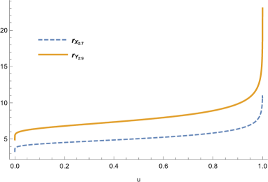
Figure 4: Plots of hazard rate functions of $X_{2:7}[Y_{2:9}]$, for all $x=-\ln u$ and $u\in(0,1]$.

5 Concluding remarks

In this paper, we study stochastic comparisons on the second-order statistics from heterogeneous dependent or independent MPHR samples. Some ordering results are established for the usual stochastic, hazard rate orderings on the second-order statistics. These new results established here provide theoretical guidance both for the winner’s prize for bid in the second-price reverse auction in auction theory and fail-safe system design in reliability theory.

Funding

This research is supported by the National Natural Science Foundation of China.

References

- Balakrishnan et al. (2017) Balakrishnan, N., Barmalzan, G., & Haidari, A. (2017). Modified proportional hazard rates and proportional reversed hazard rates models via marshall–olkin distribution and some stochastic comparisons. Journal of the Korean Statistical Society, (p. S1226319217300674).
- Balakrishnan et al. (2015) Balakrishnan, N., Haidari, A., & Barmalzan, G. (2015). Improved ordering results for fail-safe systems with exponential components. Communications in Statistics - Theory and Methods, 44, 2010–2023.
- Balakrishnan & Rao (1998) Balakrishnan, N., & Rao, C. R. (1998). Order statistics : theory methods. Handbook of Statistics, .
- Balakrishnan & Torrado (2016) Balakrishnan, N., & Torrado, N. (2016). Comparisons between largest order statistics from multiple-outlier models. Statistics, 50, 176–189.
- Balakrishnan & Zhao (2013a) Balakrishnan, N., & Zhao, P. (2013a). Ordering properties of order statistics from heterogeneous populations: A review with an emphasis on some recent developments. Probability in the Engineering Informational Sciences, 27, 403–443.
- Balakrishnan & Zhao (2013b) Balakrishnan, N., & Zhao, P. (2013b). Ordering properties of order statistics from heterogeneous populations: a review with an emphasis on some recent developments. Probability in the Engineering and Informational Sciences, 27, 403–443.
- Barmalzan et al. (2016) Barmalzan, G., Najafabadi, A. T. P., & Balakrishnan, N. (2016). Likelihood ratio and dispersive orders for smallest order statistics and smallest claim amounts from heterogeneous weibull sample. Statistics & Probability Letters, 110, 1–7.
- Barmalzan et al. (2019) Barmalzan, G., Najafabadi, A. T. P., & Balakrishnan, N. (2019). Ordering results for series and parallel systems comprising heterogeneous exponentiated weibull components. Communications in Statistics-Theory and Methods, 48, 660–675.
- Belzunce et al. (2016) Belzunce, F., Riquelme, C. M., & Mulero, J. (2016). An introduction to stochastic orders. Academic Press.
- Bon & Paltanea (2006) Bon, J. L., & Paltanea, E. (2006). Comparison of order statistics in a random sequence to the same statistics with i.i.d. variables. ESAIM, 10, p.1–10.
- Cai et al. (2017) Cai, X., Zhang, Y., & Zhao, P. (2017). Hazard rate ordering of the second-order statistics from multiple-outlier phr samples. Statistics, 51, 615–626.
- Das & Kayal (2021a) Das, S., & Kayal, S. (2021a). On comparison of the second-order statistics from independent and interdependent exponentiated location-scale distributed random variables. arXiv preprint arXiv:2104.08525, .
- Das & Kayal (2021b) Das, S., & Kayal, S. (2021b). Some ordering results for the marshall and olkin’s family of distributions. Communications in Mathematics and Statistics, 9, 153–179.
- Das et al. (2021) Das, S., Kayal, S., & Balakrishnan, N. (2021). Orderings of the smallest claim amounts from exponentiated location-scale models. Methodology and Computing in Applied Probability, 23, 971–999.
- Ding et al. (2013) Ding, W., Zhang, Y., & Zhao, P. (2013). Comparisons of k-out-of-n systems with heterogenous components. Statistics Probability Letters, 83, 493–502.
- Dykstra et al. (1997) Dykstra, R., Kochar, S., & Rojo, J. (1997). Stochastic comparisons of parallel systems of heterogeneous exponential components. Journal of Statistical Planning Inference, 65, 203–211.
- Embrechts (2004) Embrechts, P. (2004). Order statistics (3rd ed.), .
- (18) Gb, A., B, S., Nb, C., & Rr, D. (). Stochastic comparisons of series and parallel systems with dependent heterogeneous extended exponential components under archimedean copula - sciencedirect. Journal of Computational and Applied Mathematics, 380.
- Ghitany (2006) Ghitany, M. E. (2006). Marshall-olkin extended pareto distribution and its application. int.j.appl.math, 18, 17–31.
- Ghitany et al. (2007) Ghitany, M. E., Al-Awadhi, F. A., & Alkhalfan, L. A. (2007). Marshall–olkin extended lomax distribution and its application to censored data. Communications in Statistics Theory Methods, 36, 1855–1866.
- Johnson et al. (1994) Johnson, N. L., Kotz, S., & Balakrishnan, N. (1994). Continuous univariate distributions, volume 1, 2nd edition, .
- Johnson et al. (1995) Johnson, N. L., Kotz, S., & Balakrishnan, N. (1995). Continuous univariate distributions. Technometrics, 22.
- Kamps (1998) Kamps, U. (1998). 10 characterizations of distributions by recurrence relations and identities for moments of order statistics. Handbook of Statistics, 16, 291–311.
- Khaledi et al. (2000) Khaledi, Baha-Eldin, Kochar, & Subhash (2000). Some new results on stochastic comparisons of parallel systems. Journal of Applied Probability, 37, 1123–1123.
- Kochar & Xu (2007) Kochar, S., & Xu, M. (2007). Stochastic comparisons of parallel systems when components have proportional hazard rates. Probability in the Engineering Informational Sciences, 21, 597–609.
- Kundu et al. (2016) Kundu, A., Chowdhury, S., Nanda, A. K., & Hazra, N. K. (2016). Some results on majorization and their applications. Journal of Computational and Applied Mathematics, .
- Li (2005) Li, X. (2005). A note on expected rent in auction theory. Operations Research Letters, 33, 531–534.
- Li & Peng (2006) Li, X., & Peng, Z. (2006). Some aging properties of the residual life of -out-of- systems. IEEE Transactions on Reliability, 55, 535–541.
- MARSHALL et al. (1997) MARSHALL, ALBERT, W., OLKIN, & INGRAM (1997). A new method for adding a parameter to a family of distributions with application to the exponential and weibull families. Biometrika, .
- Marshall et al. (1979) Marshall, A. W., Olkin, I., & Arnold, B. C. (1979). Inequalities: theory of majorization and its applications volume 143. Springer.
- Marshall & IngramOlkin (2007) Marshall, B., & IngramOlkin (2007). Life Distributions. Life Distributions.
- Mudholkar & Srivastava (1993) Mudholkar, G. S., & Srivastava, D. K. (1993). Exponentiated weibull family for analyzing bathtub failure-rate data. IEEE Transactions on Reliability, 42, 299–302.
- Navarro & Shaked (2010) Navarro, J., & Shaked, M. (2010). Some properties of the minimum and the maximum of random variables with joint logconcave distributions. Metrika, 71, 313–317.
- Navarro et al. (2017) Navarro, J., Torrado, N., & águila, Y. d. (2017). Comparisons between largest order statistics from multiple-outlier models with dependence. Methodology Computing in Applied Probability, .
- Nelsen (2006) Nelsen, R. B. (2006). An Introduction to Copulas (Springer Series in Statistics) volume 47. Springer-Verlag Berlin, Heidelberg.
- Păltănea (2008) Păltănea, E. (2008). On the comparison in hazard rate ordering of fail-safe systems. Journal of Statistical Planning and Inference, 138, 1993–1997.
- Paul & Gutierrez (2004) Paul, A., & Gutierrez, G. (2004). Mean sample spacings, sample size and variability in an auction-theoretic framework. Operations Research Letters, 32, 103–108.
- Pledger & Proschan (1971) Pledger, G., & Proschan, F. (1971). Comparisons of order statistics and of spacings from heterogeneous distributions. Optimizing Methods in Statistics, (pp. 89–113).
- Proschan & Sethuraman (1976) Proschan, F., & Sethuraman, J. (1976). Stochastic comparisons of order statistics from heterogeneous populations, with applications in reliability. Journal of Multivariate Analysis, 6, 608–616.
- Rojo & Kochar (1996) Rojo, J., & Kochar, S. C. (1996). Some new results on stochastic comparisons of spacings from heterogeneous exponential distributions. Journal of Multivariate Analysis, .
- Shaked & Shanthikumar (2007) Shaked, M., & Shanthikumar, G. (2007). Stochastic orders. Springer Science Business Media.
- SUBHASH KOCHARMAOCHAO (2011) SUBHASH KOCHARMAOCHAO, X. U. (2011). On the skewness of order statistics in multiple-outlier models. Journal of Applied Probability, 48, 271–284.
- Torrado (2015) Torrado, N. (2015). On magnitude orderings between smallest order statistics from heterogeneous beta distributions. Journal of Mathematical Analysis and Applications, 426, 824–838.
- Torrado & Kochar (2015) Torrado, N., & Kochar, S. C. (2015). Stochastic order relations among parallel systems from weibull distributions. Journal of Applied Probability, 52, 102–116.
- Zhang et al. (2021) Zhang, M., Lu, B., & Yan, R. (2021). Ordering results of extreme order statistics from dependent and heterogeneous modified proportional (reversed) hazard variables. AIMS Mathematics, 6, 584–606.
- Zhao & Balakrishnan (2009) Zhao, P., & Balakrishnan, N. (2009). Mean residual life order of convolutions of heterogeneous exponential random variables. Journal of Multivariate Analysis, 100, 1792–1801.
- Zhao & Balakrishnan (2010) Zhao, P., & Balakrishnan, N. (2010). Dispersive ordering of fail-safe systems with heterogeneous exponential components. Metrika, 74, 203–210.
- Zhao et al. (2011) Zhao, P., Li, X., & Da, G. (2011). Right spread order of the second-order statistic from heterogeneous exponential random variables. Communications in Statistics - Theory and Methods, 40, 3070–3081.
- Zhao & Zhang (2014) Zhao, P., & Zhang, Y. (2014). On the maxima of heterogeneous gamma variables with different shape and scale parameters. METRIKA, 77, 811–836.