The long road to calibrated prediction uncertainty in computational chemistry

Abstract

Uncertainty quantification (UQ) in computational chemistry (CC) is still in its infancy. Very few CC methods are designed to provide a confidence level on their predictions, and most users still rely improperly on the mean absolute error as an accuracy metric. The development of reliable UQ methods is essential, notably for CC to be used confidently in industrial processes. A review of the CC-UQ literature shows that there is no common standard procedure to report or validate prediction uncertainty. I consider here analysis tools using concepts (calibration and sharpness) developed in meteorology and machine learning for the validation of probabilistic forecasters. These tools are adapted to CC-UQ and applied to datasets of prediction uncertainties provided by composite methods, Bayesian Ensembles methods, machine learning and a posteriori statistical methods.

I Introduction

As stated in recent perspective articles (Lejaeghere2020, ; Rommel2021, ; Reiher2022, ), uncertainty quantification (UQ) in computational chemistry (CC) is still in its early stages of development. For instance, in electronic structure theory, at the exception of the BEEF-type methods (Wellendorff2014, ), none of the methods implemented in popular computational chemistry codes provides an uncertainty or a confidence index on the calculated properties. Confidence is generally based on benchmark studies which provide performance indices, such as the ubiquitous mean absolute error (MAE). However, it is well established that, lacking a probabilistic interpretation, the MAE should not be used as an uncertainty proxy (Ruscic2014, ; Pernot2015, ; Pernot2018, ). As will be seen below, prediction uncertainty might be much more complex to estimate than usual performance indices.

This difficulty in quantifying our confidence in model predictions has far reaching consequences. It is an obstacle for computational chemistry to stand on par with, or to replace, physical measurements (Irikura2004, ) or to be used in decision making (Wan2021, ). It also has a strong impact on multi-scale simulation, where propagation of uncertainty through the scales is necessary to assess the reliability of predictions (Gabriel2021, ; Mao2021, ; Ye2021, ), or in iterative learning to minimize the cost of high-level calculations (Proppe2016, ; Simm2016, ; Hie2020, ). In benchmarking, a very sensible way to select among a set of levels of theory would be to pick one with a fit-to-purpose prediction uncertainty. It is also worth to note that uncertainty provides a metric for the comparison of measurement values, a prerequisite to the production of reproducible results (Volodina2021, ). In all such applications, a prediction uncertainty estimate has to be fair: underestimation is potentially dangerous (overconfidence), and overestimation is wasteful. Reaching a good balance is the main challenge of UQ.

For the purpose of the present study, I sorted UQ approaches into two classes, according to their embedding level within the computational chemistry method:

• Embedded UQ methods produce prediction uncertainty concurrently with property predictions. This is an heterogeneous class which presently encompasses the above-mentioned BEEF or Bayesian Ensemble approach (Wellendorff2014, ) and several bottom-up correction methods with detailed uncertainty budgets (the Type B methods of Ruscic (Ruscic2014, )), such as the Feller-Peterson-Dixon method (Feller2008, ; Feller2017, ) or the ATOMIC protocol (Bakowies2019, ; Bakowies2020, ; Bakowies2021, ). Some machine learning methods, such as Bayesian neural networks which are designed to provide uncertainty along with prediction, also belong here (Tran2020, ; Gawlikowski2021, ). These methods are akin to the “molecule-specific” UQ concept (Reiher2022, ).

• A-posteriori UQ methods use a set of predictions and a reference dataset to estimate prediction uncertainty, generally after trend correction (Pernot2011, ; Lejaeghere2014, ; Lejaeghere2014a, ; Lejaeghere2016, ; DeWaele2016, ; Pernot2015, ; Proppe2017, ; Lejaeghere2020, ). This is sometimes referred to as “the statistical approach”, albeit statistical tools are also at the heart of embedded methods. Ruscic defined it as the Type A method (Ruscic2014, ). Some examples, at various sophistication levels, are the correction of harmonic vibrational frequencies by scaling factors (Scott1996, ; Pernot2011, ), regression analysis of various properties (Faver2011b, ; Lejaeghere2014, ; Lejaeghere2014a, ; Pernot2015, ; Proppe2016, ; Proppe2017, ; Das2021, ), correction by Gaussian Processes (Kennedy2001, ; Proppe2019a, ) and $\Delta$-Machine Learning ($\Delta$-ML) methods (Ramakrishnan2015, ; Tran2020, ; Nandi2021, ; Unzueta2021, ; Bhattacharjee2021, ; Hruska2022, ).

Very often, the validation of prediction uncertainty values provided by these CC-UQ methods is based on the qualitative appreciation of the agreement of prediction uncertainty with the amplitude of errors (Csontos2010, ; DeWaele2016, ). For the Bayesian ensemble methods, calibration has been assessed by a visual examination of the normality of $z$-scores histograms (Mortensen2005, ), or by visual evaluation of the width of error bars (Wellendorff2012, ; Wellendorff2014, ). When quantitative tools have been used, notably for the validation of a-posteriori methods, a popular test statistic is the prediction interval coverage probability (PICP) (Shrestha2006, ; Gawlikowski2021, ). PICP tests have been done either on the full dataset (Proppe2017, ; Proppe2021, ; Bakowies2021, ), or using a splitting scheme between calibration and validation sets (Pernot2015, ; Proppe2021, ). Globally, there does not seem to be (yet) a consensus in the community on the adequate validation vocabulary, concepts and tools, which would be necessary to compare the merits of different CC-UQ strategies.

In the past few decades, probabilistic forecasting for meteorology has been the object of fundamental developments of validation concepts and methods (Gneiting2007a, ; Gneiting2014, ). Two major concepts resulting from these studies are calibration (reliability), and sharpness (resolution). A probabilistic prediction method is said to be calibrated if the confidence of predictions matches the probability of being correct for all confidence levels (Tomani2020, ). A calibrated method is sharp if it produces the tightest possible confidence intervals (Kuleshov2018, ). Sharpness is conditional on calibration (a method cannot be sharp if it is not calibrated). With the emergence of prediction uncertainty estimation in Machine Learning, several calibration and sharpness metrics, and graphical checks are also now used in this field (Kuleshov2018, ; Tran2020, ; Lai2021, ; Gawlikowski2021, ).

Most computational chemistry methods are based on deterministic algorithms, but our lack of knowledge about their prediction errors links them to probabilistic forecasters. Part of these validation tools have recently been introduced to the computational chemistry field by Tran et al. (Tran2020, ) to compare the calibration and sharpness of several ML algorithms trained to predict adsorption energies. This is, to my knowledge the only study of this kind in the application field of interest. My intent in this study is to adapt and apply calibration/sharpness validation methods to a wider computational chemistry domain, and to evaluate their pertinence in various scenarios, with the expectation that such methods could be more generally used in the community.

In the Sec. II, I review the specifics of CC-UQ (error sources, UQ methods) and previous validation practices. I then present (Sec. III) the panel of validation tools for probabilistic forecasters (calibration and sharpness metrics and graphical checks), and I propose adapted methods for the typical CC-UQ outputs. In Sec. IV, these tools are applied to a variety of datasets. The main features of this study are reported and discussed in the conclusions (Sec. V).

II The computational chemistry UQ context

A major obstacle to UQ in computational chemistry is the predominant role of systematic errors. As uncertainty is a non-negative parameter expected to quantify unpredictable errors (GUM, ), estimation (and correction) of predictable or systematic errors is a challenging, but necessary preliminary step to CC-UQ. The international reference guide for metrology (a.k.a. ’the GUM’ (GUM, )) states that “It is assumed that the result of a measurement has been corrected for all recognized significant systematic effects and that every effort has been made to identify such effects.” (GUM, Sect. 3.2.4). As a consequence, the partition between unpredictable and predictable errors depends on the efforts that a modeler is ready or able to invest in the analysis.

I next consider the main sources of errors in computational chemistry (Sect. II.1) and the existing UQ methods, based on different approaches to systematic error corrections (Sect. II.2).

II.1 Error sources in computational chemistry

The main error sources in computational chemistry have been reviewed recently (Lejaeghere2020, ; Rommel2021, ), and can be tagged as numerical, parametric, and model errors. I come back briefly on these categories in order to discuss the expected errors distributions, which is an essential ingredient to define UQ validation methods.

II.1.1 Numerical Errors

These include errors due to finite arithmetics implementation of computational chemistry codes and, for stochastic methods, to the random errors resulting from finite sampling. For properly implemented and converged methods, numerical errors can often be assumed to be well controlled and negligible against other error sources (Irikura2004, ) (except for instances of numerical chaos (Feher2012, ; Lafage2020, )). However, for most algorithms we are still missing rigorous error bounds (Cances2017, ; Herbst2020, ), and estimation of the amplitude of numerical errors due to finite arithmetics requires computational approaches. In the Monte Carlo framework, one observes the effects of tiny perturbations of model inputs (Irikura2004, ; Feher2012, ) and/or arithmetic operations (Scott2007, ; Denis2016, ; Chatelain2019, ), without need to alter the codes. The use of interval arithmetics has also been proposed (Janes2011, ), but it might require in-depth recoding, barely an option for legacy computational chemistry codes. This is however not a fatality for newly developed codes, as shown recently by Herbst et al. (Herbst2020, ) with the development of a DFT code in the Julia language accepting arbitrary floating point types, including intervals. For some parameters, the amplitude of numerical errors can also be estimated by systematic convergence studies (Carbogno2021, ).

One can consider numerical errors as random variables, but their distribution is not necessarily normal. Non-normal distributions occur, for instance, for rounding errors in floating point arithmetics (Higham2019, ), or stochastic errors for Quantities of Interest (QoIs) in molecular dynamics (Wan2021, ).

II.1.2 Parametric errors

These occur in methods involving the statistical estimation of parameters with respect to reference data (e.g., semi-empirical force-fields, extrapolation schemes in composite methods, semi-empirical methods, statistical corrections…). An essential property of parametric errors is that their amplitude should decrease when the size of the reference dataset increases. The amplitude of parametric errors is typically estimated by Monte Carlo uncertainty propagation, from a probability density function of the parameters obtained, for instance, by Bayesian inference (Cailliez2011, ; Cailliez2020, ).

The distribution of parametric errors depends on the distribution of the uncertain parameters and on the functional form of the model with respect to these parameters. Here again, normality cannot be assumed as a default distribution feature.

II.1.3 Model errors

For computational chemistry, model errors include level-of-theory errors (e.g., the choice of a density functional approximation, DFA) and representation errors (e.g., the choice of a basis set or discretization grid). They are often the dominant contributions to a computational chemistry uncertainty budget. Compared to numerical and parametric errors, which are mostly aleatoric, model errors are systematic. The estimation and correction of model errors are usually handled either by bottom-up approaches of physics-based corrections (Ruscic2014, ), or by corrective statistical models (the so-called discrepancy functions (Kennedy2001, )) involving the comparison with a dataset of reference results (Pernot2017, ). It is important to note that, in contrast to parametric errors, model errors do not decrease when the size of the reference dataset increases.

Model errors can present any type of distribution (Pernot2018, ). However, a recent study on the shape of error distributions for different QoIs and DFAs showed that the distributions are most often unimodal, with various levels of asymmetry, and that they are in most cases heavier-tailed than a normal distribution (Pernot2021, ).

II.2 Main error correction and prediction uncertainty estimation methods

I review here the main methods appearing in the CC-UQ literature to correct systematic errors and estimate prediction uncertainty, focusing on the level of information they are able to provide, which goes from a standard uncertainty to a full distributions of predictions.

II.2.1 Bottom-up correction methods

Proceeding from a chosen level-of-theory/representation and applying successive corrections based on physical criteria is a systematic way to establish an uncertainty budget: each correction, being imperfect, coming with some uncertainty. This kind of approach is referred to as “Type B methods” by Ruscic (Ruscic2014, ), in reference to the method defined in the GUM (GUM, ) for the estimation of uncertainty in the absence of a statistical sample (statistical analysis of data samples defines Type A methods (Ruscic2014, ; Klippenstein2017a, )). It appears however that some form of Type A analysis lies at the heart of some bottom-up correction methods. For instance, the Feller-Peterson-Dixon (FPD) method considers two main uncertainty components: the complete basis-set (CBS) and the zero-point energy (ZPE) corrections. For the CBS correction, uncertainty is estimated as the half-spread of the corrections provided by five different extrapolation models (Feller2008, ). For ZPE, it is taken as half the difference in the last step of a series of approximations (Feller2012, ). I note for further reference that in the FPD approach uncertainties are combined linearly instead of quadratically, a worst case scenario ignoring possible error compensations (Feller2006, ). This is expected to provide a “crude but conservative uncertainty”, from which the estimation of prediction intervals is not straightforward and complicates the interpretation of calibration tests.

In contrast, the ATOMIC composite method aims “to provide realistic corrections and uncertainty estimates corresponding to intervals of 95% confidence…” (Bakowies2019, ). Here, a mixture of linear and quadratic uncertainty combination is used in deriving the final uncertainty. Bakowies (Bakowies2020, ) summarizes the interest of the bottom-up correction approach: “The proposed model is a welcome alternative to statistical assessment, first because it does not depend on comparison with experiment, second because it recognizes the expected scaling of error with system size, and third because it provides a detailed account of the importance of various contributions to overall error and uncertainty.“

II.2.2 A-posteriori prediction uncertainty estimation

A-posteriori approaches elaborate a statistical model independent of the computational chemistry method to estimate its prediction uncertainty, generally after correction of the original model predictions for systematic errors (Pernot2011, ; Pernot2015, ; Vishwakarma2021, ; Das2021, ). As for bottom-up corrections, different prediction uncertainty estimation models are necessary for different predicted properties by a given method.

The a-posteriori approach requires three elements:

1. A reference dataset on which to calibrate the statistical model, the ideal being a large set (at least several hundreds) of high-accuracy values.

2. A statistical model to correct the (systematic) trends in the model errors. This optional step might involve from a simple shift to machine learning models.

3. A statistical method to estimate the prediction uncertainty from the residual errors, the complexity of which depends on their distribution.

If a trend correction is applied (step 2), it is important to note that the a-posteriori approach does not provide a prediction uncertainty for the original computational chemistry method, but for its corrected version. This has been clearly illustrated for the correction of vibrational frequencies by scaling factors (Pernot2011, ), or for the linear correction of DFT-predicted Mössbauer isomer shifts (Proppe2017, ).

One can point out two main obstacles to the success of the a-posteriori approach, affecting the first and third steps:

• The reference dataset should contain as many as possible high-accuracy data, which, depending on the studied property, might be difficult to achieve, notably for experimental data. For the application of simple correction models, the errors dataset should also be homogeneous, in the sense that it should not contain multiple contradictory trends preventing the success of step 2. This might be less stringent for machine learning correction models, which should be able to correct for multiple trends, provided a relevant set of input features. In addition, care should be taken that the prediction uncertainty is corrected from reference data uncertainty (Pernot2015, ; Klippenstein2017a, ), a problem absent from bottom-up correction methods.

• The ability to establish reliable prediction uncertainties heavily relies on the distribution of the corrected errors. Skewed or heteroscedastic error distributions (i.e., where the variance of the errors varies along the predictor variable) might be specifically challenging for the definition of an uncertainty. The difficulty to establish and communicate asymmetric and/or heteroscedastic uncertainty might even be considered as a criterion to reject some computational chemistry methods for prediction uncertainty estimation.

A-posteriori methods have been mostly used to estimate standard uncertainties or prediction intervals. Depending on the approach, a full distribution might be accessible (e.g., for regression models, Gaussian processes…).

II.2.3 Bayesian ensemble methods

In the DFT framework, the Bayesian Error Estimation density Functional (BEEF) family of methods has been designed to provide uncertainty on its predictions (Mortensen2005, ; Medford2014, ; Ulissi2017, ; Houchins2017, ; Guan2019, ).

In a first step, the parameters of a DFA are calibrated by Bayesian inference against a reference dataset. However, the resulting parametric uncertainties are typically insufficient to cover the amplitude of prediction errors (remember that the amplitude of parametric errors decreases with the size of the calibration dataset).

To restore the validity of the statistical model, the variance-covariance matrix of the reference data is scaled by a ’temperature’ factor such that the mean prediction variance matches the variance of prediction errors (Wellendorff2012, ). The resulting probability density function (pdf) of the DFA parameters is captured as an ensemble of parameters values which can then be used to estimate prediction uncertainty on any relevant property by Monte Carlo sampling. Note that, as Bayesian ensembles are calibrated to cover the amplitude of prediction errors, their prediction uncertainty is affected by reference data uncertainty. When comparing predictions to experimental values, care should be taken not to count experimental uncertainty twice.

In the available literature the results of BEEF models are summarized by a mean value and a standard deviation and the ensembles are not used for validation.

II.2.4 Machine learning

Materials science and catalysis see an intensive development of ML algorithms to replace DFT calculations (Montavon2013, ; Ramakrishnan2014, ; Ramakrishnan2015, ; Rupp2015, ; Faber2017, ; Ulissi2017, ; Zaspel2019, ; Tran2020, ; CesardeAzevedo2021, ; Duan2021, ; Nandi2021, ; Venkatraman2021, ). DFT error correction by ML models is also a pathway actively explored to obtain high accuracy results from low-level DFT calculations (Ramakrishnan2015, ; Bhattacharjee2021, ; Nandi2021, ; Unzueta2021, ).

UQ is central to many automatized applications in screening or design of efficient compounds, and several ML algorithms are now available to estimate prediction uncertainty, through either distribution- or ensemble-based methods. A recent comparison of the calibration and sharpness of these methods by Tran et al. (Tran2020, ) reveals a wide spectrum of reliability of ML-UQ methods.

III Methods for the validation of prediction uncertainty

The general framework for the validation of probabilistic predictions is first presented to define the calibration and sharpness concepts and the associated statistical test and metrics. The cases with restricted information, in the shape of an uncertainty (standard or expanded) instead of a full distribution, are then considered, for which validation methods are derived from the general framework. The concepts are illustrated on synthetic data.

III.1 General case: probabilistic predictions

A probabilistic prediction provides a distribution over the values that can be taken by the Quantity of Interest (QoI), $V$. The predicted cumulative distribution function (CDF) for $V$ is noted $F(V)$ and the reciprocal quantile function $F^{-1}(p)\equiv F_{p}^{-1}$, where $p$ is a probability. For the sake of validation, predictions are made for a series of $M$ test systems for which one has reference values $\{R_{i}\}_{i=1}^{M}$. For each reference system $i$, one has thus a predicted CDF $F_{i}(V)$ and the corresponding quantile function $F_{p,i}^{-1}$.

Few UQ methods provide prediction distributions, and approximations of CDF functions are often available through ensembles of values, representative of the predictive distribution. Such ensembles are generated by ML-UQ methods, Bayesian Ensemble BEEF-type methods or stochastic algorithms.

III.1.1 Definitions: Calibration and sharpness

A method is considered to be calibrated (or reliable) if the confidence of predictions matches the probability of being correct for all confidence levels (Tomani2020, ; Tran2020, ). Formally, the empirical and predicted CDFs should be identical (Kuleshov2018, ), i.e.

$$\lim_{M\rightarrow\infty}\frac{1}{M}\sum_{i=1}^{M}\boldsymbol{1}\left(R_{i}\leq F_{p,i}^{-1}\right)=p,\,\forall p\in[0,1]$$ (1)

where $\boldsymbol{1}(x)$ is the indicator function for proposition $x$, taking values 1 when $x$ is true and 0 when $x$ is false. This equation can be generalized to prediction intervals (Kuleshov2018, )

$$\lim_{M\rightarrow\infty}\frac{1}{M}\sum_{i=1}^{M}\boldsymbol{1}\left(R_{i}\in I_{p,i}\right)=p,\,\forall p\in[0,1]$$ (2)

where

$$I_{p,i}=\left[F_{(1-p)/2,i}^{-1},F_{(1+p)/2,i}^{-1}\right]$$ (3)

is the 100$p$ % prediction interval for the predicted value $V_{i}$.

However, this calibration condition is not sufficient to ensure that the prediction uncertainties or confidence intervals are useful. Eqs. 1-2 provide an average calibration assessment over the test set, but does not guarantee that calibration is realized locally for each predicted value. A useful prediction model must also be sharp, i.e., prediction intervals should be as tight as possible around any predicted value (Kuleshov2018, ).

Example

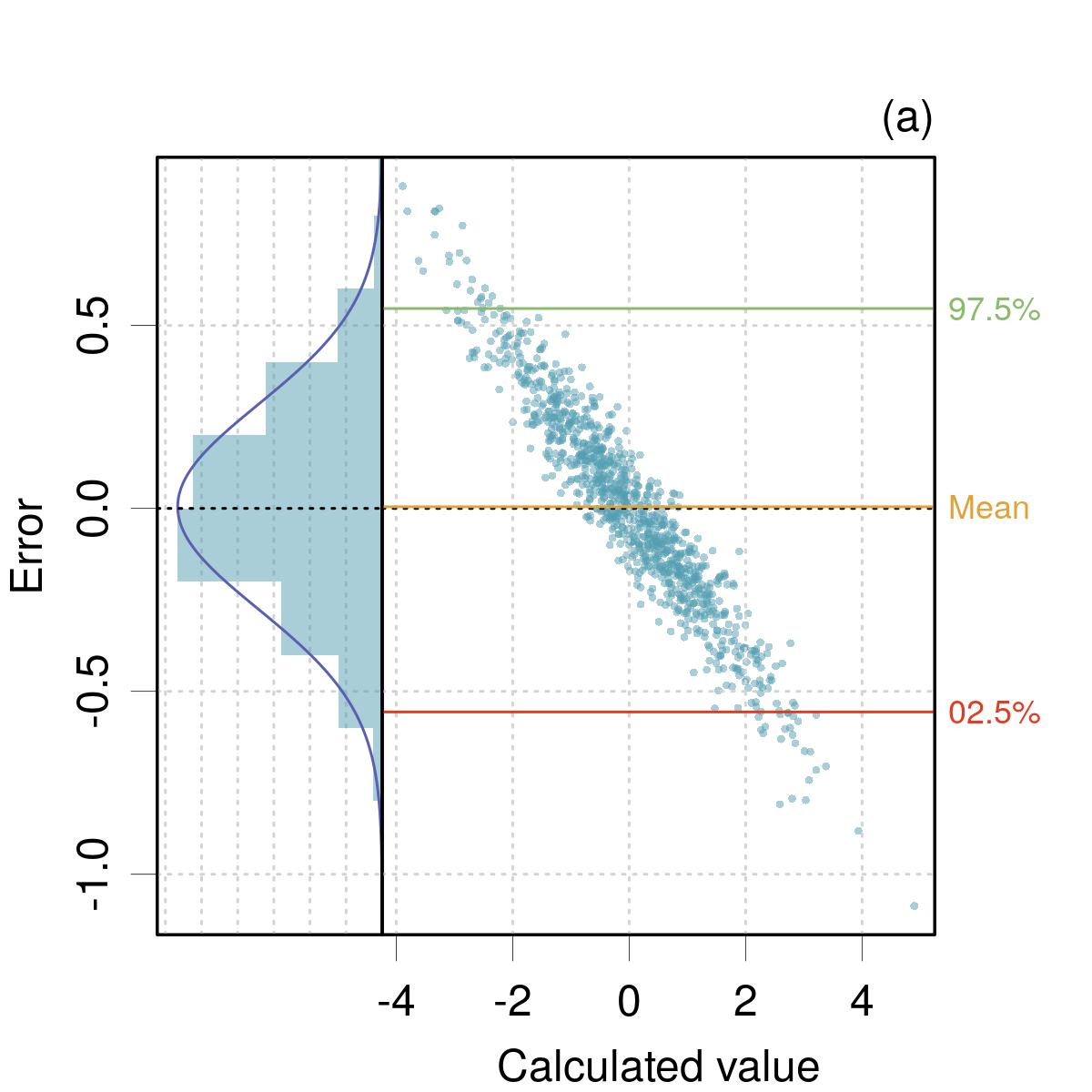
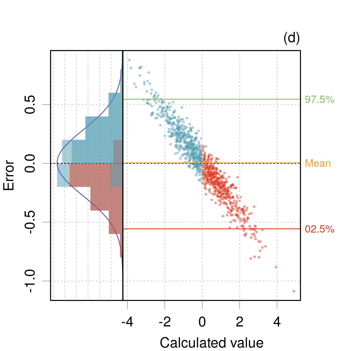
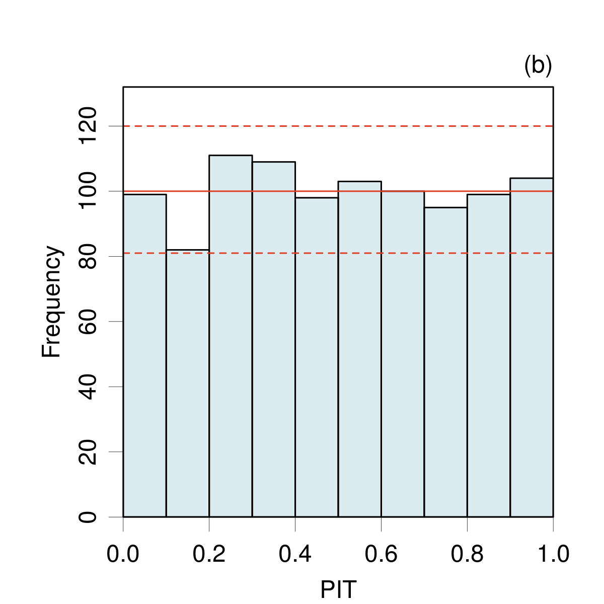
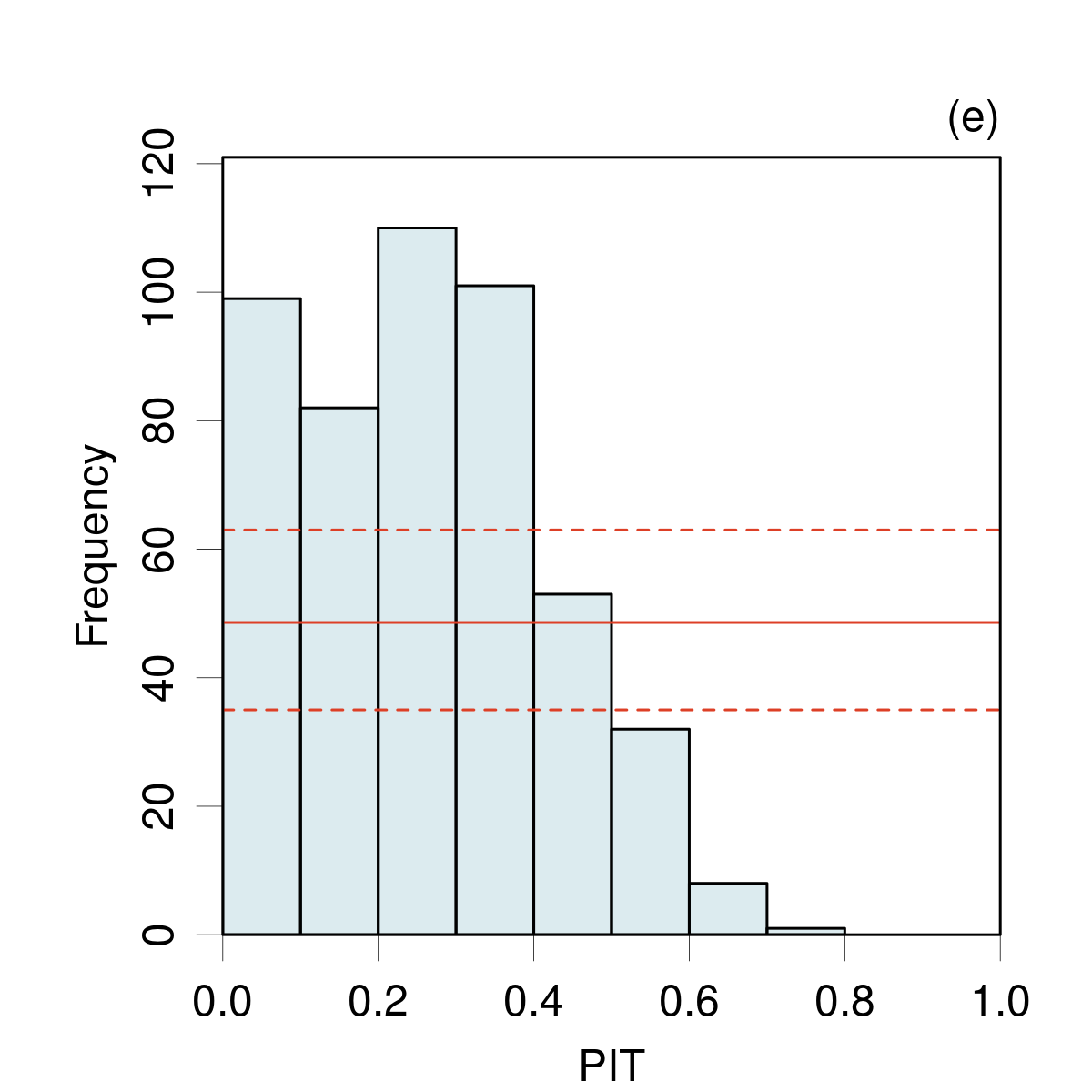
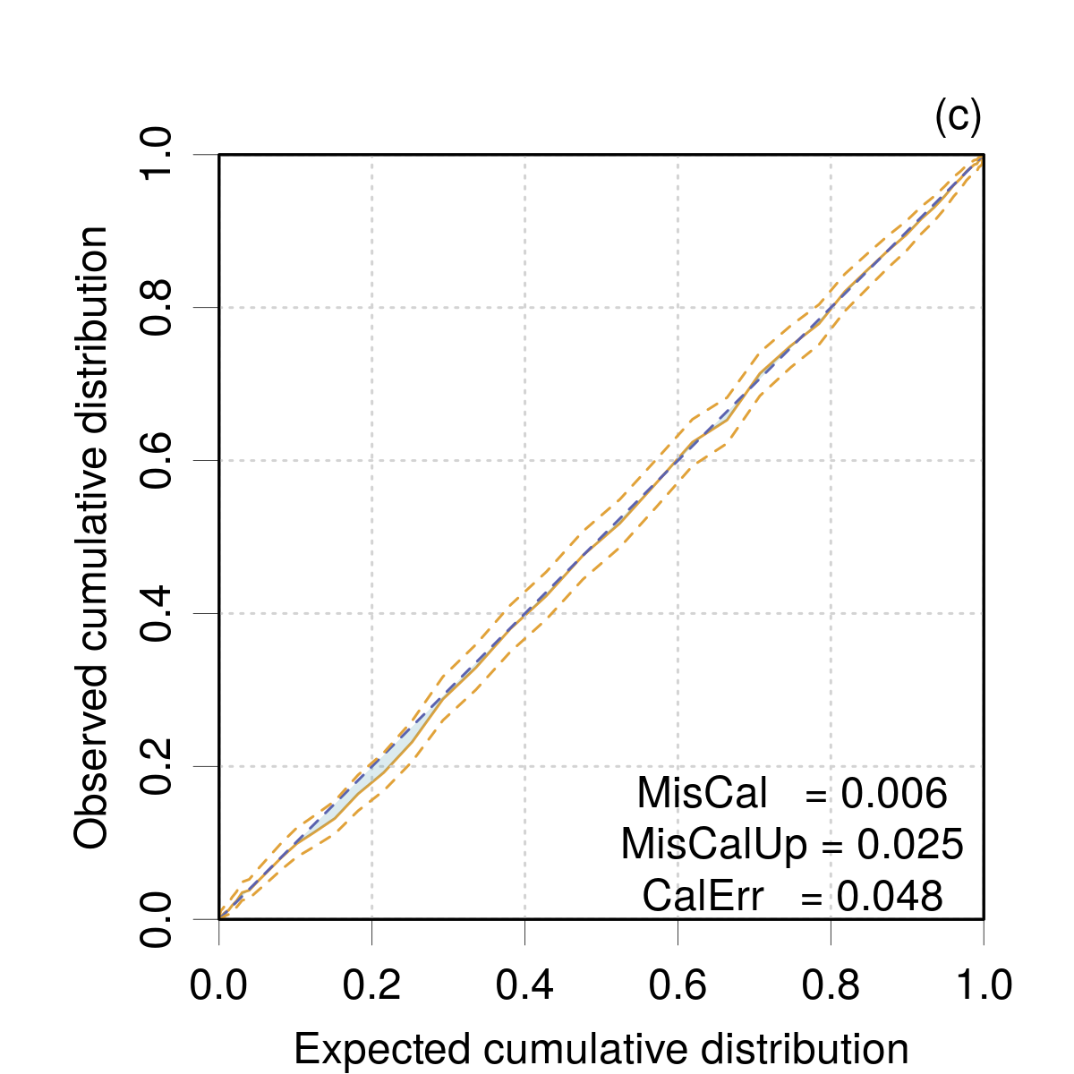
Let us consider a toy model where the predictive CDF $F(V)$ is learned from an ensemble of errors $E_{i}=R_{i}-V_{i}$ with uncorrected bias and without accounting for the linear dependence of $E$ on $V$ (Fig. 1(a)). Figure 1: Error samples from a normal distribution with a linear trend: (a,d) Error distribution plots; (b,e) Probability integral transform (PIT) histograms; (c,f) Calibration curves. In (d-f), the uncertainty statistics estimated over the whole dataset are used to validate a subset restricted to the positive calculated values (red dots). Assuming that the test set has the same properties as the learning set, using the system-independent $F_{p}^{-1}$ function will provide correct prediction intervals over the test set, and Eqs. 1-2 will be satisfied. However, if $F_{p}^{-1}$ is used to design prediction intervals for a local subset of the test set, for instance the positive values of $V$ ((Fig. 1(d)), the intervals will clearly be oversized and ill-centered: sharpness will not be ensured. In the first case, calibration tests such as the probability integral transform (PIT) histogram presented below (Sect. III.1.2) do not detect a problem (Fig. 1(b)), while the same test on the local subset of the data is diagnostic of a calibration problem (Fig. 1(e)).

III.1.2 Calibration tests and metrics

Several visual checks and statistics have been proposed to estimate calibration and sharpness of probabilistic predictions (Cook2006, ; Gneiting2007a, ; Gneiting2014, ; Kuleshov2018, ). I review below the most pertinent ones for CC-UQ applications and extend the toolbox with a graphical representation enabling to assess simultaneously average and local calibration. Some of these tools have been used in a ML setup, where statistical uncertainty on the validation statistics is negligible; this is not the case in a typical CC-UQ problem, so I added confidence intervals to all estimators.

Probability integral transform histogram.

The probability integral transform (PIT) is the value that the predictive CDF attains at a test value $R_{i}$ (Gneiting2014, )

$$PIT_{i}=F_{i}(R_{i})$$ (4)

For a calibrated method, a histogram of the PIT values for the validation set should be uniform over [0,1]. The PIT histogram enables a visual check of Eq. 1, which does not require additional information.

Due to the finite size $M$ of the validation set, one should not expect a perfectly uniform histogram. In order to assess significant deviations from the uniform distribution, a 95 % confidence interval on the bin heights in a uniform histogram is obtained from the quantiles of the Poisson distribution with rate $M/n_{bin}$ where $n_{bin}$ is the number of bins in the PIT histogram. Significant deformations of the histogram from a uniform distribution can be used to diagnose calibration problems (see the Supplementary Material, Sec. III). Alternatively or in complement to this graphical check (Sailynoja2021, ), some authors recommend statistical tests for uniformity (Cook2006, ).

Example (continued)

PIT histograms are shown in Fig. 1(b,e). For the first one, the binned PIT values stand in the confidence range for a uniform histogram, assessing the calibration of the predictions. A contrario, the second histogram presents significant deviations from the uniform, with an excess of small values pointing to a negative bias in the predictions.

Calibration curve.

Calibration can also be checked by comparing the estimated success rate in the left hand side of Eq. 1

$$\eta_{p}=\frac{1}{M}\sum_{i=1}^{M}\boldsymbol{1}\left(R_{i}\leq F_{p,i}^{-1}\right)$$ (5)

to the target probability $p$ for a series of $p$ values in $[0,1]$. By plotting $\eta_{p}$ vs $p$, one gets a calibration curve (Kuleshov2018, ; Tran2020, ). For a calibrated method, the curve should lie on the identity line. Note that calibration curves might also be designed from Eq. 2, but testing small coverage intervals does not seem very pertinent in a UQ setup.

To account for finite $M$ values and assess the overlap of the calibration curve with the identity line, a 95 % confidence band is plotted around the calibration curve (see Sec. III.4.1 for implementation details). As for the PIT histogram, deformations of the calibration curve from the identity line are diagnostic of calibration problems (see the Supplementary Material, Sec. III).

Miscalibration area and calibration error.

The area between the calibration curve and the identity line (miscalibration area, noted MisCal (Tran2020, )) can be used as a calibration metric. To use it for testing, we consider as an upper limit half of the area of the 95 % confidence band around the curve (MisCalUp): if MisCal $>$ MisCalUp, the identity line does not lie within the 95 % confidence band, and calibration can be questioned.

A calibration error (CalErr) is also proposed in the literature, as the sum of squared differences over the probabilities in the calibration curve (Kuleshov2018, ), or its square root (Tran2020, ). The latter is retained here for its homogeneity with an error. As MisCal, it can be used to compare several methods on their calibration level.

Example (continued)

Fig. 1(c,f) shows the calibration curves corresponding to both scenarios in Fig. 1(a,b). The one corresponding to the full calibration dataset does not deviate notably from the identity line, and the MisCal statistic is much smaller that its upper limit MisCalUp. In the second case, there is no ambiguity about miscalibration, for either the curve or the statistics. As a confirmation, the calibration error in the second case (CalErr$=1.3$) is much larger than in the first case ($0.048$).

PICP testing for a series of target coverage probabilities.

The effective coverage of a $100p$ % prediction interval $I_{p}$ is estimated by its prediction interval coverage probability (PICP) (Shrestha2006, ; Gawlikowski2021, ), as the ratio of $S_{p}$, the number of successes ($R_{i}\in I_{p,i}$) , to the size $M$ of the validation set

$$\nu_{p}=S_{p}/M$$ (6)

where

$$S_{p}=\sum_{i=1}^{M}\boldsymbol{1}\left(R_{i}\in I_{p,i}\right)$$

To test if a PICP value $\nu_{p}$ is compatible with the target coverage probability $p$, one checks if $p$ lies within a 95 % confidence interval around $\nu_{p}$ (see Section III.4.1 for implementation details).

Direct application of Eq. 2 would lead to test PICP values for a regular set of coverage probabilities in $[0,1]$. However, one is typically interested in large coverage values, and there is little practical interest to consider low-probability intervals. In the following, I will consider $p=0.5$ (inter-quartile range), $0.75$ and $0.95$.

III.1.3 Sharpness metrics

Several sharpness metrics have been proposed, such as the mean prediction interval width (Lai2021, ), or the mean variance of the prediction distributions (Kuleshov2018, ). Here I retain the definition of Tran et al. (Tran2020, )

$$sha=\sqrt{\frac{1}{M}\sum_{i=1}^{M}\mathrm{Var}(F_{i})}$$ (7)

where $\mathrm{Var}(F_{i})$ is the variance associated with the CDF at point $i$, $F_{i}(V)$. $sha$ has the dimension of an uncertainty on the QoI and it corresponds to the mean prediction uncertainty (MPU) used in an earlier study by Pernot et al. (Pernot2015, ). The mean predictive variance ($sha^{2}$) has also been used as a model performance metric by Proppe at al. (Proppe2017, ), and as a calibration statistic for the BEEF methods (Wellendorff2012, ; Medford2014, ; Wellendorff2014, ).

It is considered that $sha$ should be small, but no threshold value is available to distinguish between sharp and unsharp methods. $sha$ is therefore a convenient metric to compare several methods, but not for self-standing sharpness assessment.

III.1.4 Local calibration

Local Coverage Probability (LCP).

One can check local calibration by performing PICP tests on subsets of the validation data. The simplest scenario is to split the dataset into contiguous areas of the predictor variable (typically the QoI $V$), but other splitting schemes can be considered. If prediction uncertainty is not constant, it might also be interesting to use it as a predictor variable to check its impact on local PICP estimates.

Two constraints have to be considered: (i) the subsets sizes have to remain large enough for PICP testing to have some power, and (ii) using equi-sized subsets could simplify the appreciation of multiple tests. The first constraint limits the resolution of the LCP analysis, and for small datasets, rather than splitting the dataset into small sets, one might use overlapping subsets. Whatever the splitting scheme, the LCP method proceeds as follows:

1. Choose a set of equi-sized areas of the predictor variable (contiguous or overlapping).

2. Repeat for several values of probability $p$:

   1. within each area (indexed by $k$), estimate the local PICP, $\nu_{p,k}=S_{p,k}/M_{k}$

   2. plot $\nu_{p,k}$ and its 95 % confidence interval at the center of each area.

The LCP plot enables to check (1) average calibration, from the agreement between estimated and target coverage probabilities, and (2) local calibration, from the uniformity of the estimated coverage across the local areas of the predictor variable(s).

As for PICP testing, one is mostly interested in large coverage probabilities, and I propose to check only the 0.5, 0.75 and 0.95 probability levels. Note that the LCP analysis uses $M_{k}$ values smaller than $M$. In consequence, tests on local PICPs have larger uncertainty and are more likely to be permissive, and a false impression of good calibration might arise. It is essential to keep in mind that (1) calibration should be estimated based on PICPs for the whole dataset, and (2) trends in the local PICP values with respect to the target coverage are important diagnostic features.

Example (continued)

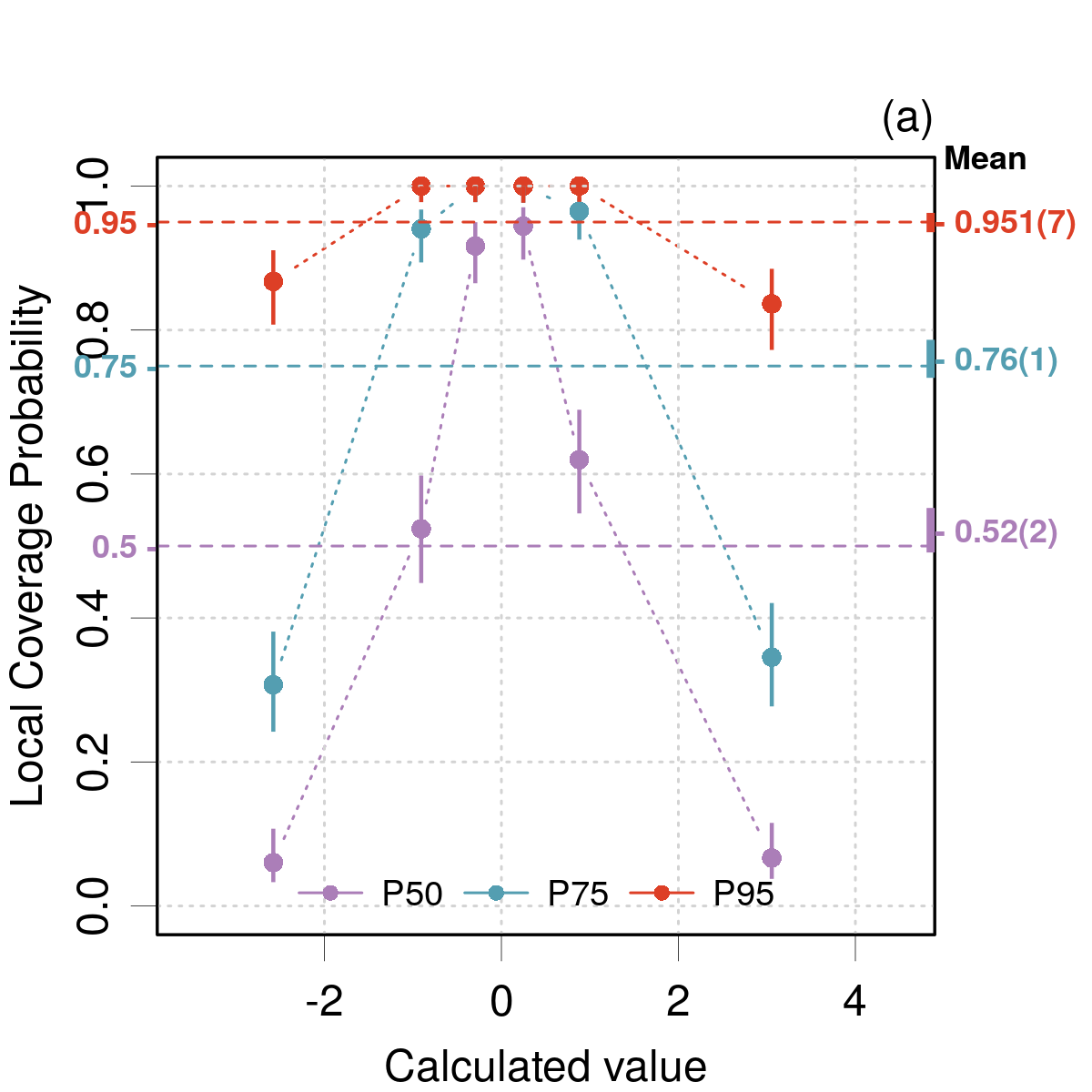
Fig. 2(a,b) shows the LCP analysis results for two scenarios. For the full set represented in Fig. 1(a), one can see in the margin of Fig. 2(a) the PICP values and their 95 % CIs, confirming the good calibration, in line with the PIT histogram, the calibration curve and statistics. In this case, the LCP procedure selects $n=\left\lfloor 1000/150\right\rfloor=6$ contiguous areas and estimates the local PICP values, which are reported at the center of each area. It is clear that the predictions are not sharp. Fig. 2(b) shows the LCP analysis for the same dataset corrected from its linear trend. In this case, the estimated prediction CDF is both calibrated and sharp. Figure 2: LCP analysis: (a) the same dataset as in Fig. 1(a); (b) after linear trend correction.

III.2 Validation of expanded uncertainty

The majority of CC-UQ methods do not provide a prediction CDF ($F_{i}$), but limited summary statistics, such as sets of predicted values $V_{i}\pm u_{V,i}$. In order to use validation methods based on Eqs. 1-2, one would have to make assumptions on the underlying CDFs. As we have seen that there is no typical shape for the computational chemistry errors distributions (Sect. II.1), it is preferable to avoid such assumptions and derive distribution-free validation methods. Let us see how the elementary test in Eq. 2

$$R_{i} \in I_{p,i}$$ (8)

can be implemented in such cases.

Assuming the symmetry of the prediction interval, one can write

$$I_{p,i}=\left[V_{i}-U_{p,i},V_{i}+U_{p,i}\right]$$ (9)

where $U_{p,i}$ is the expanded prediction uncertainty at the $p$ level. Eq. 8 is therefore equivalent to

$$|E_{i}|\leq U_{p,i}$$ (10)

where $E_{i}=R_{i}-V_{i}$ is an error. Note the $U_{p}$ should account for both calculation and reference errors.

Hence, when an expanded prediction uncertainty for the errors – typically $U_{95,i}$ – is available, on can consider Eq. 10 without hypothesis on the errors distribution other than symmetry and the ones made to estimate $U_{p,i}$. This enables us to use PICP testing (Sect. III.1.2) and the LCP analysis for sharpness.

III.3 Validation of standard uncertainty using $z$-scores

When a standard uncertainty $u_{E,i}$ is available, Eq. 10 can be rewritten as

$$|E_{i}|\leq f_{p,i}u_{E,i}$$ (11)

where $f_{p,i}$ is a coverage factor associated with the errors CDF $F_{i}$, at point $i$. Considering that the errors distribution strongly depends on the dominant error source in a calculation, it is often difficult to define the errors CDF on which to estimate coverage factors. In such cases, it might be interesting to directly test the consistency of the errors and uncertainties through their ratio, as shown below.

Let us assume that we have unbiased errors with unknown distribution, but known standard deviation $\sigma_{i}>0$,

$$\mathrm{E}(E_{i}) =0$$ (12)

$$\mathrm{Var}(E_{i}) =\sigma_{i}^{2}$$ (13)

Then, the $z$-scores, $z_{i}=E_{i}/\sigma_{i}$, are unit-scaled and zero-centered variables, i.e.,

$$\mathrm{E}(z_{i}) =\mathrm{E}(E_{i})/\sigma_{i}=0$$ (14)

$$\mathrm{Var}(z_{i}) =\mathrm{Var}(E_{i})/\sigma_{i}^{2}=1$$ (15)

Therefore, if the errors are unbiased and the $\sigma_{i}$ values are correctly estimated by $u_{E,i}$, the distribution of $z$-scores should be unbiased with unit variance,

$$\mathrm{E}(Z) =0$$ (16)

$$\mathrm{Var}(Z) =1$$ (17)

In the absence of information on the $z$-score distribution, testing the value of $\mathrm{Var}(Z)$ cannot be done using the popular chi-squared test, which is not robust with respect to deviations from the underlying normality assumption (Supplementary Material, Sec. II). As for the PICP, the $z$-score variance is tested against a 95 % confidence interval (estimated by bootstrapping; see Sect. III.4.2).

III.3.1 Local $z$-score variance (LZV) analysis

Similar to the LCP analysis for coverage probabilities (Sect. III.1.3), I propose a local analysis based on the variance of $z$-scores, estimated in a series of contiguous or overlapping areas [Local z-score Variance (LZV) analysis]. For each subset, $\mathrm{Var}(Z)$ and its 95% confidence interval are estimated and plotted on a graph. Intervals that do not cross the unity variance line might be considered as problematic, but here also, trends are of diagnostic interest.

Example

A dataset of errors has been generated in the hypothesis of a Student’s-$t$ errors distribution ($\mathcal{T}(\nu)$) and non-uniform random variances issued from a chi-squared distribution ($\chi^{2}(\nu)$) scaled to have unit mean

$$E_{i} =u_{E,i}\sqrt{3/5}\mathcal{T}(\nu=5)$$ (18)

$$u_{E,i} =0.01\sqrt{s_{i}/<s>}$$ (19)

$$s_{i} \sim\chi^{2}(\nu=4)$$ (20)

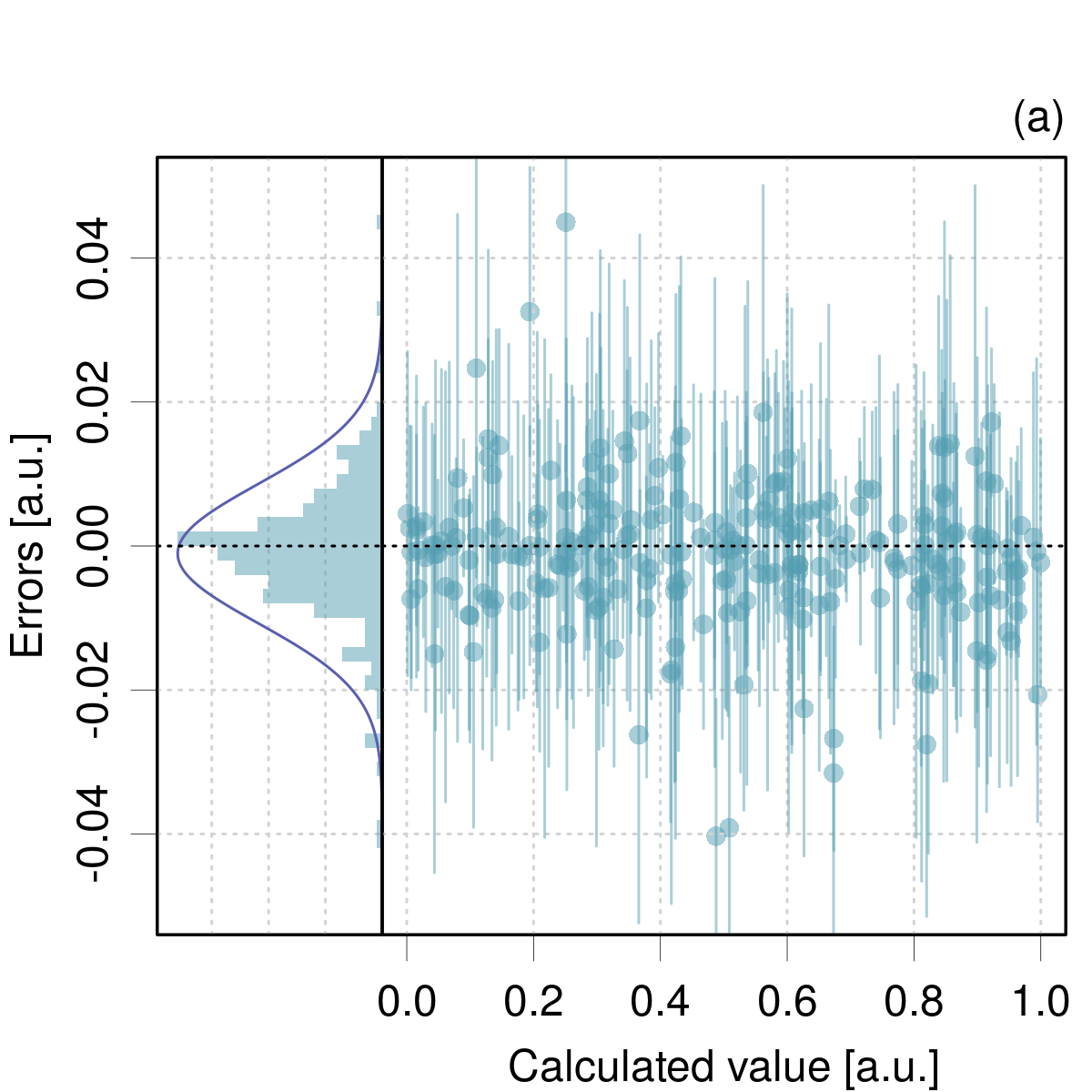
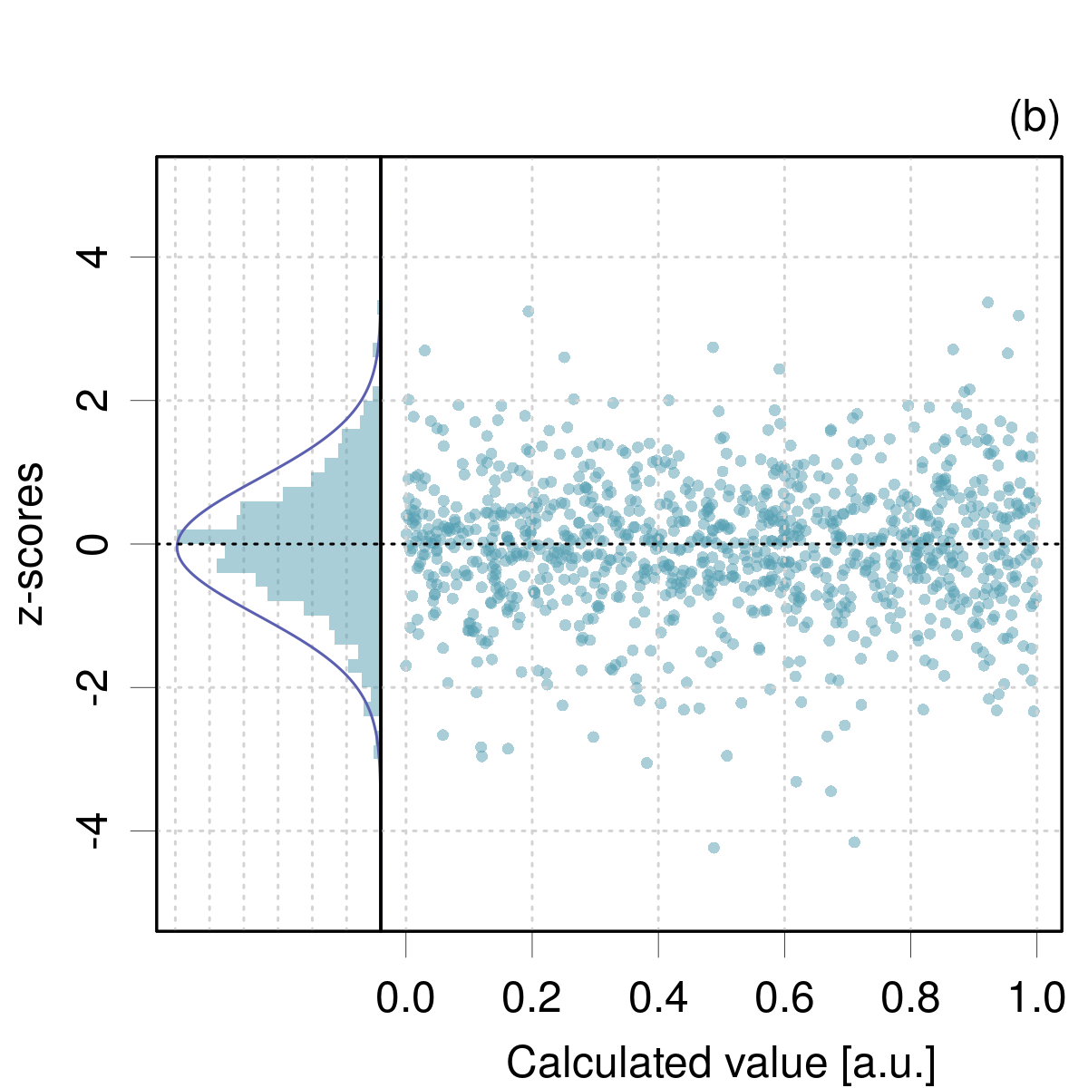
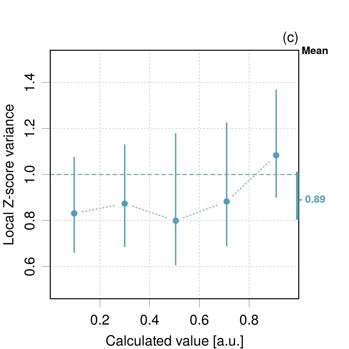
The errors and $z$-scores distributions for a sample of $N=1000$ $z$-scores are shown in Fig. 3(a,b). The $z$-score statistics are $\mathrm{E}(Z)=-0.045(30)$ and $\mathrm{Var}(Z)=0.894(53)$, with a 95 % probability interval equal to $\left[0.8,1.0\right]$ for the variance, which is validated. Figure 3: Toy model error distribution generated from Eqs. 18-20 with $N=1000$: (a) thinned subset ($N=250$) and $1.96*u_{E}$ for the error bars; (b) full set of $z$-scores; (c) and (d) LZV analysis of the $z$-scores with respect to the calculated value (c) and the prediction uncertainty (d).

The LZV analysis has been performed along the calculated values (Fig. 3(c)) and along the prediction uncertainty (Fig. 3(d)), using five areas of 200 points. Both graphs show the compatibility of the $z$-scores with the unity variance requirement, and no remarkable trend is observed.

III.4 Implementation

III.4.1 Binomial proportions confidence intervals

As presented in Sec. I of the Supplementary Material about PICP testing, the discreteness of binomial proportions $\nu_{p}$ and the asymmetry of the associated confidence intervals make the estimation of binomial proportions confidence intervals a complex problem. Numerous methods are available, from which I retained the continuity corrected Wilson method for this study (Newcombe1998, ).

Sec. I of the Supplementary Material also reports considerations about the power of PICP testing. For instance, to reject the hypothesis that a PICP value $\nu=0.99$ is equal to the target coverage $p=0.95$, one needs at least $M=150$ points to achieve a power of 0.8. This has to be taken into account for the LCP analysis, where I adopt a systematic strategy to find a balance between testing power and resolution: the number of subsets is taken as $n=\left\lfloor M/150\right\rfloor$ and constrained to lie between 2 and 15. If the number of subsets is smaller than 5, a sliding window of size $M/n$ is used.

III.4.2 Testing $z$-scores variance

In order to test the variance of $z$-scores with respect to the target value (1), Sec. II of the Supplementary Material concludes on the use of a bootstrapping method, with the limits of a 95 % confidence intervals estimated by the BC_a method (DiCiccio1996, ). The design parameters for the LZV analysis are the same as for the LCP analysis.

III.4.3 Code availability

Graphical functions plotPIT, plotCalCurve, plotLZV and plotLCP have been included in ErrViewLib-v1.4 https://github.com/ppernot/ErrViewLib/releases/tag/v1.4, also available in Zenodo at https://doi.org/10.5281/zenodo.5817888.

IV Applications

The tools and statistics presented above for the validation of prediction uncertainty estimates are applied below to several datasets extracted from the literature or provided by kind colleagues. The choice of datasets is subjective, mostly guided by availability and complementarity in methods and properties. They cover the major embedded and a-posteriori CC-UQ methods. These datasets are available online at https://github.com/ppernot/PU2022, or in Zenodo at https://doi.org/10.5281/zenodo.5818026.

IV.1 Datasets with expanded prediction uncertainty

Despite the recommendations of Ruscic(Ruscic2014, ) for the systematic use of $U_{95}$ expanded uncertainty in reference databases(Klippenstein2017a, ), I did not find many CC-UQ studies providing them explicitly for a reasonable dataset size. I selected two recent studies in which I found considerations about prediction sharpness.

IV.1.1 Expanded uncertainty of errors

The ideal scenario is to have sets of predictions and reference data with their expanded uncertainties: $V_{i}$, $U_{95;i}^{(V)}$, $R_{i}$ and $U_{95,i}^{(R)}$. The estimation of the errors and their associated expanded uncertainty using the combination of variances requires the hypothesis that the expansion factors for predictions and reference values have similar values ($f_{95,i}^{(R)}\simeq f_{95,i}^{(V)}$), leading to

$$U_{95,i}=\sqrt{(U_{95,i}^{(R)})^{2}+(U_{95,i}^{(V)})^{2}}$$ (21)

It is then directly possible to test the PICP value

$$\nu_{0.95}=\frac{1}{M}\sum_{i=1}^{M}\boldsymbol{1}\left(|E_{i}|/U_{95,i}\leq 1\right)$$ (22)

leading to a single assessment of calibration at the $p=0.95$ level.

When the uncertainties of the reference data are negligible, this approach directly tests the quality of the expanded uncertainties for the predicted values $U_{95}^{(V)}$. Otherwise, the quality of the reference set uncertainties $U_{95}^{(R)}$ will also affect the results.

IV.1.2 The BAK2021 dataset

Bakowies and von Lilienfeld (Bakowies2021, ) proposed a new method to estimate zero-point energies (ZPE) and the corresponding expanded $U_{95}$ uncertainty in the framework of the composite ATOMIC method. Interestingly, they observed a quadratic dependence of the ZPE scaling factors and their dispersion with the fraction of heteroatoms in a set of 279 molecules. From this, they built a statistical model for 95 % prediction intervals, and they validated this heteroscedastic expanded uncertainty on a set of 99 molecules against CCSD(T) ZPE values, by looking for outlying points. They did not identify any concern about the predicted prediction intervals and conclude that their method “provides a fair estimate of 95 % confidence” (Bakowies2021, ).

This is a small dataset ($N=99$), and I find interesting to check how the validation tools perform in this context. The values for the ATOMIC-2(um) and CCSD(T) ZPE data were manually (and painstakingly) extracted from Table S6 of the Supporting Information of the original article (Bakowies2021, ). There is no uncertainty on the reference values for this dataset. The errors distribution is shown in Fig. 4(a).

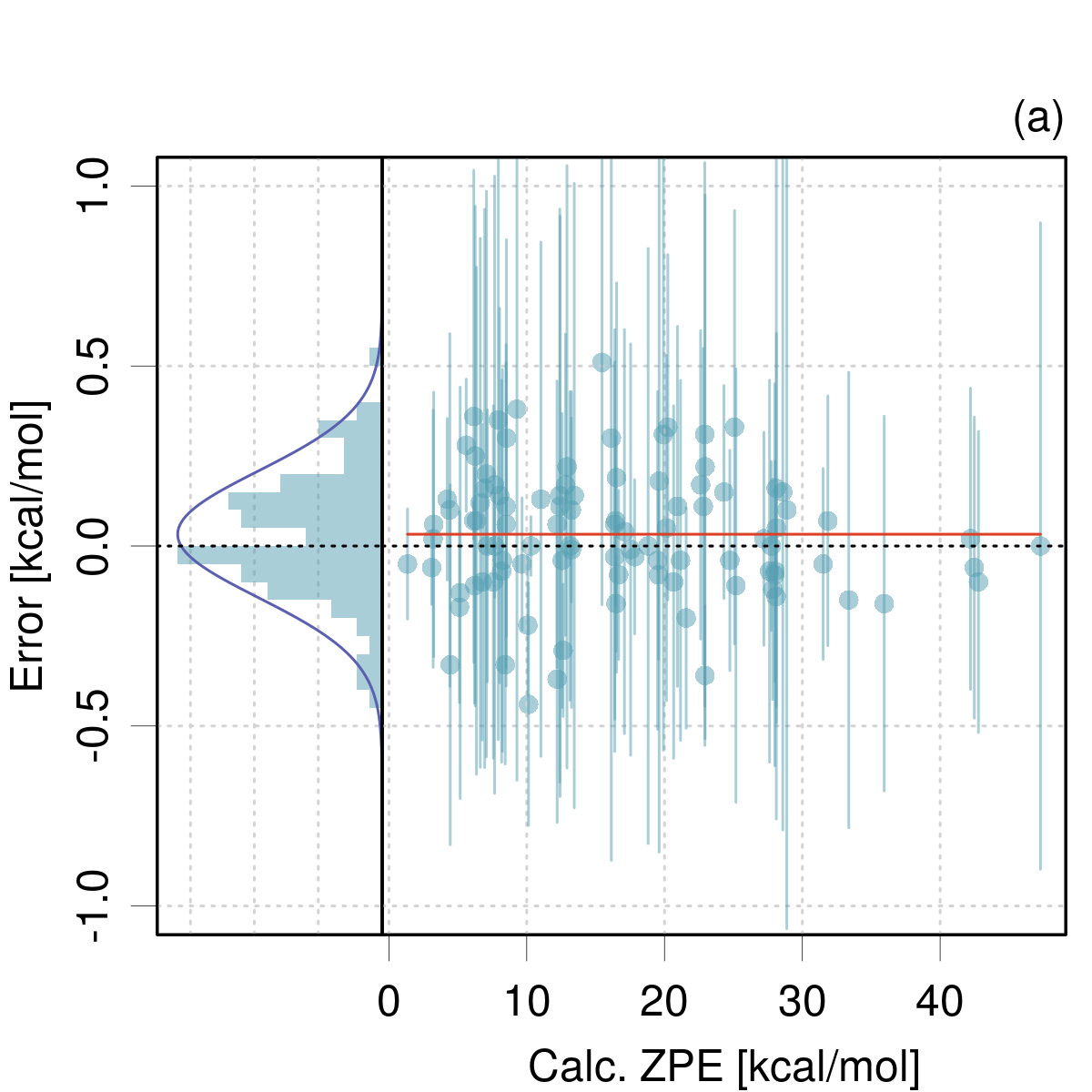
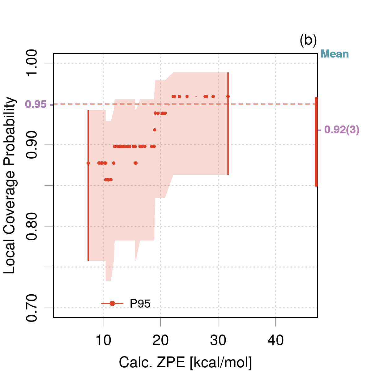
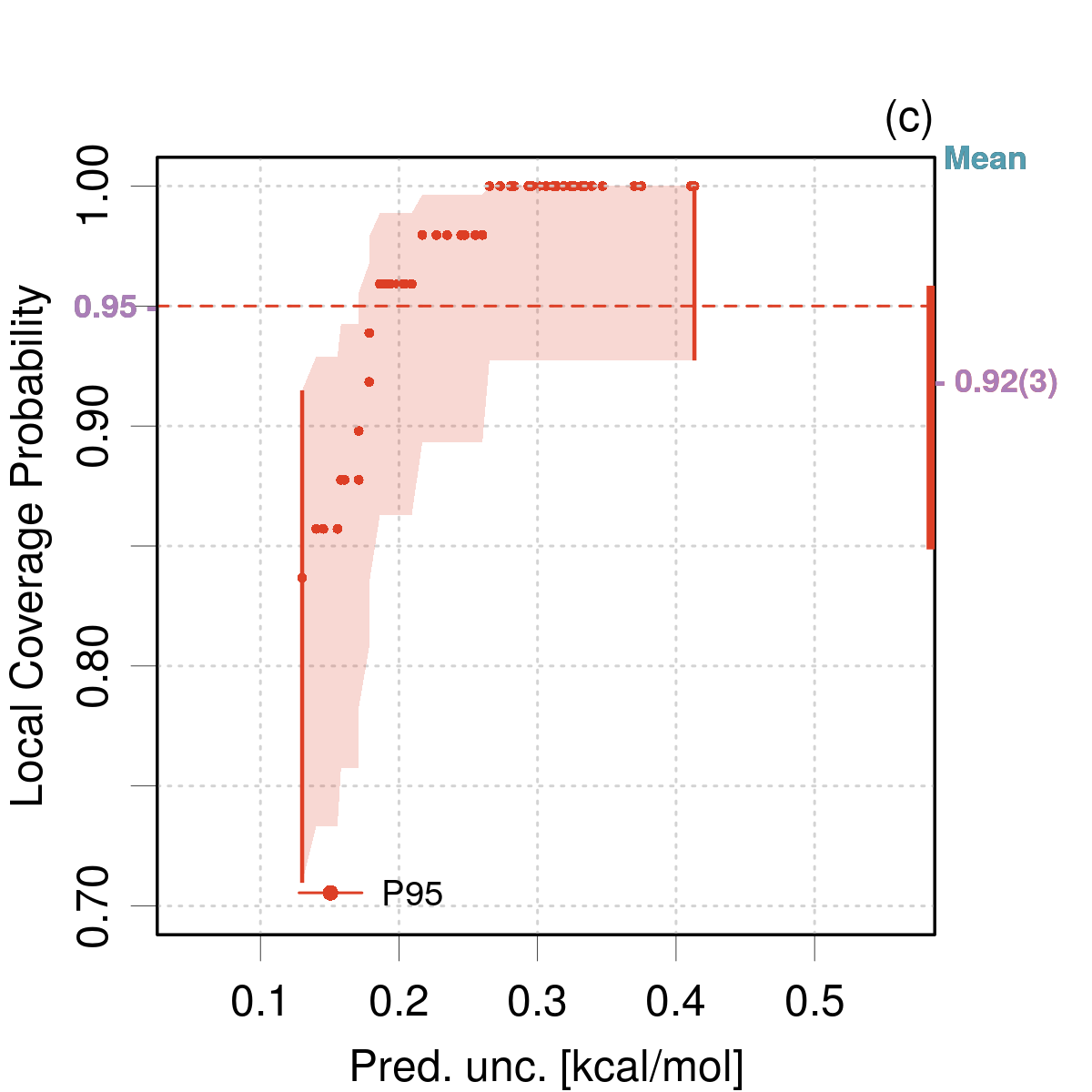
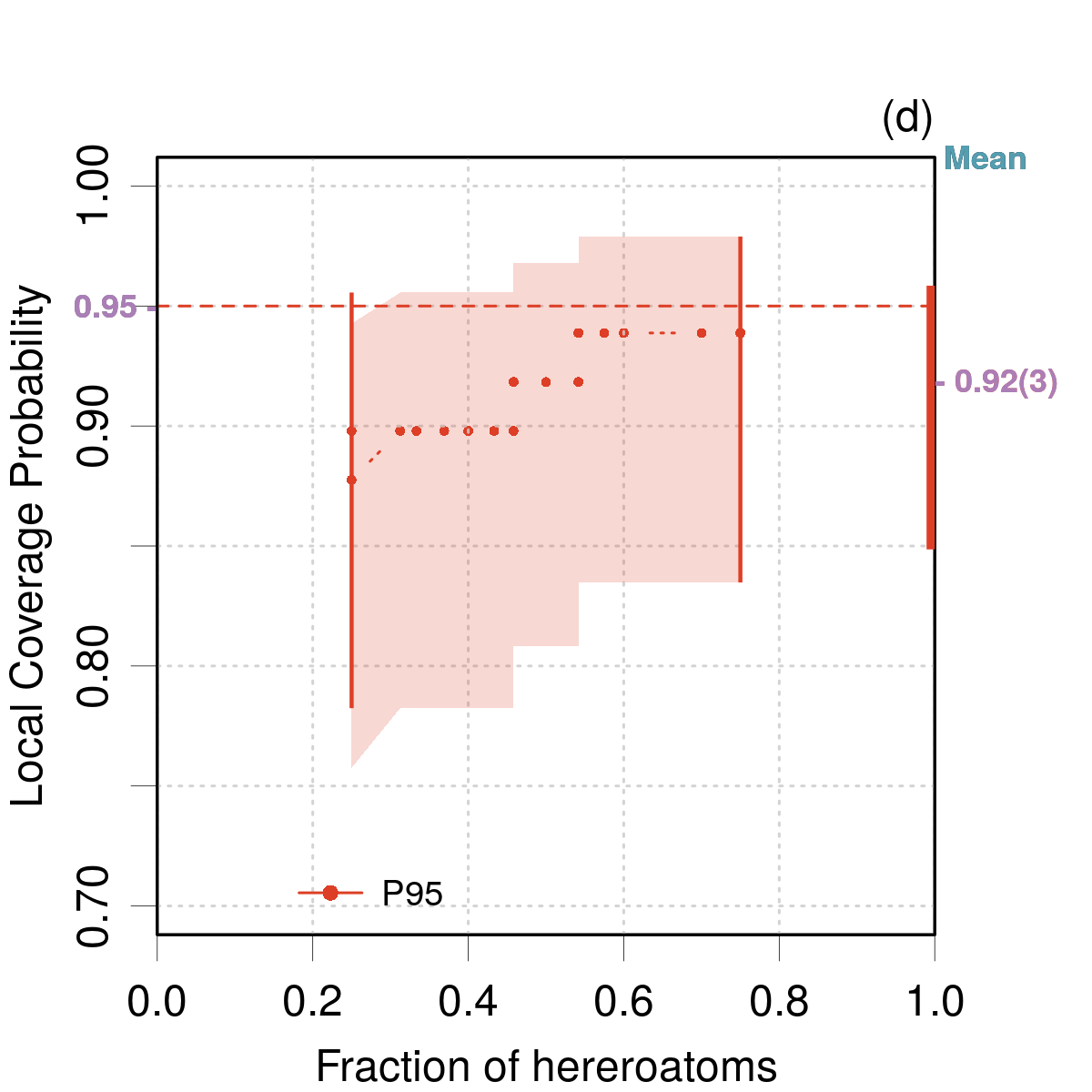
Figure 4: Distribution of errors (a) and alternative versions of LCP analysis (b)-(d) for the BAK2021 dataset. The LCP analysis has been done using (b) the calculated value, (c) the prediction uncertainty and (d) the heteroatoms content, as predictor variables.

Considering that expanded $U_{95}$ uncertainties are reported, I tested only this probability level. The global PICP $\nu_{0.95}=0.92(3)$ is not significantly different from the target value.

Three alternative versions of the LCP analysis are tested. The LCP areas have been chosen along the calculated ZPE values (Fig. 4(b)), the estimated prediction uncertainty (Fig. 4(c)) and the heteroatoms content of the molecules (Fig. 4(d)). Because of the small dataset, a sliding window of width $M=N/2$ was used in all cases. Despite the large error bars, a few points indicate a statistical rejection of local PICP values. In ZPE space (Fig. 4(b)), one notices a global trend, with PICP values increasing from 0.89 to 0.96 as the ZPE value increases. This might reveal an underestimation of the uncertainties for small ZPE values. An analogous trend is observed in prediction uncertainty space (Fig. 4(c)), with PICP values increasing from 0.84 to 1. This would indicate that small prediction uncertainties are too small, and large ones too large. The third representation is along the property that was used to design the prediction uncertainty model (Fig. 4(d)), and the positive trend, although still present, is much weaker than in the ZPE or prediction uncertainty space.

Overall, one can agree with Bakowies and von Lilienfeld that their UQ method globally provides “fair” $U_{95}$ values, but with a caveat about a local calibration issue, as revealed in the PU-space LCP analysis.

IV.1.3 The PRO2021 dataset

In a recent study, Proppe and Kircher (Proppe2021, ) estimated prediction uncertainty for reaction rates derived by the Mayr-Patz equation. Their uncertainty model accounts for parametric uncertainty and model discrepancy, for which they compared two versions. In the first version (a), the model dispersion is uniform (homoscedastic), whereas in the second version (b), it has a polynomial dependence on the parametric uncertainty. Using graphs showing the correlation between prediction uncertainty and dispersion of the residuals (their Fig. 5), Proppe and Kircher conclude that the second version offers a much better fit to the residuals distribution (better sharpness). However, both models provide 95 % prediction intervals with an excessive 99 % coverage.

The authors kindly provided me the corresponding datasets containing $M=212$ points with a reference value (log of the experimental reaction rate), a calculated value (log of the calculated reaction rate) and an expanded uncertainty on the error, for both model versions (a) and (b). No further data treatment was necessary. The distribution of errors and their expanded uncertainties is shown in Fig. 5(a) for method (a). There is no easily perceptible difference on the same plot for method (b), which is not shown.

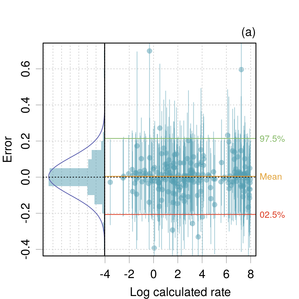
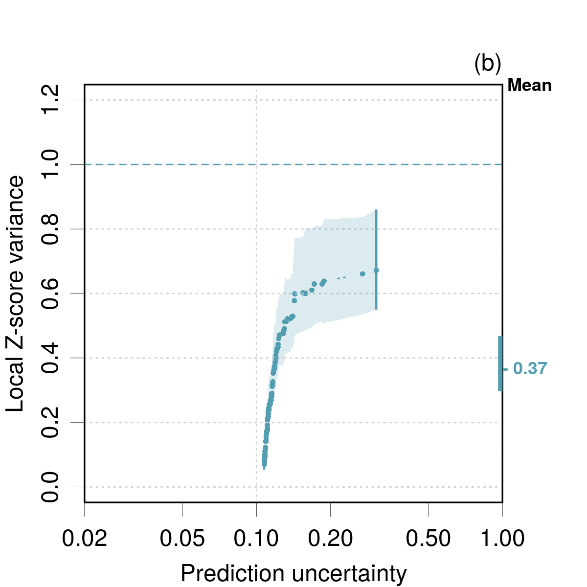
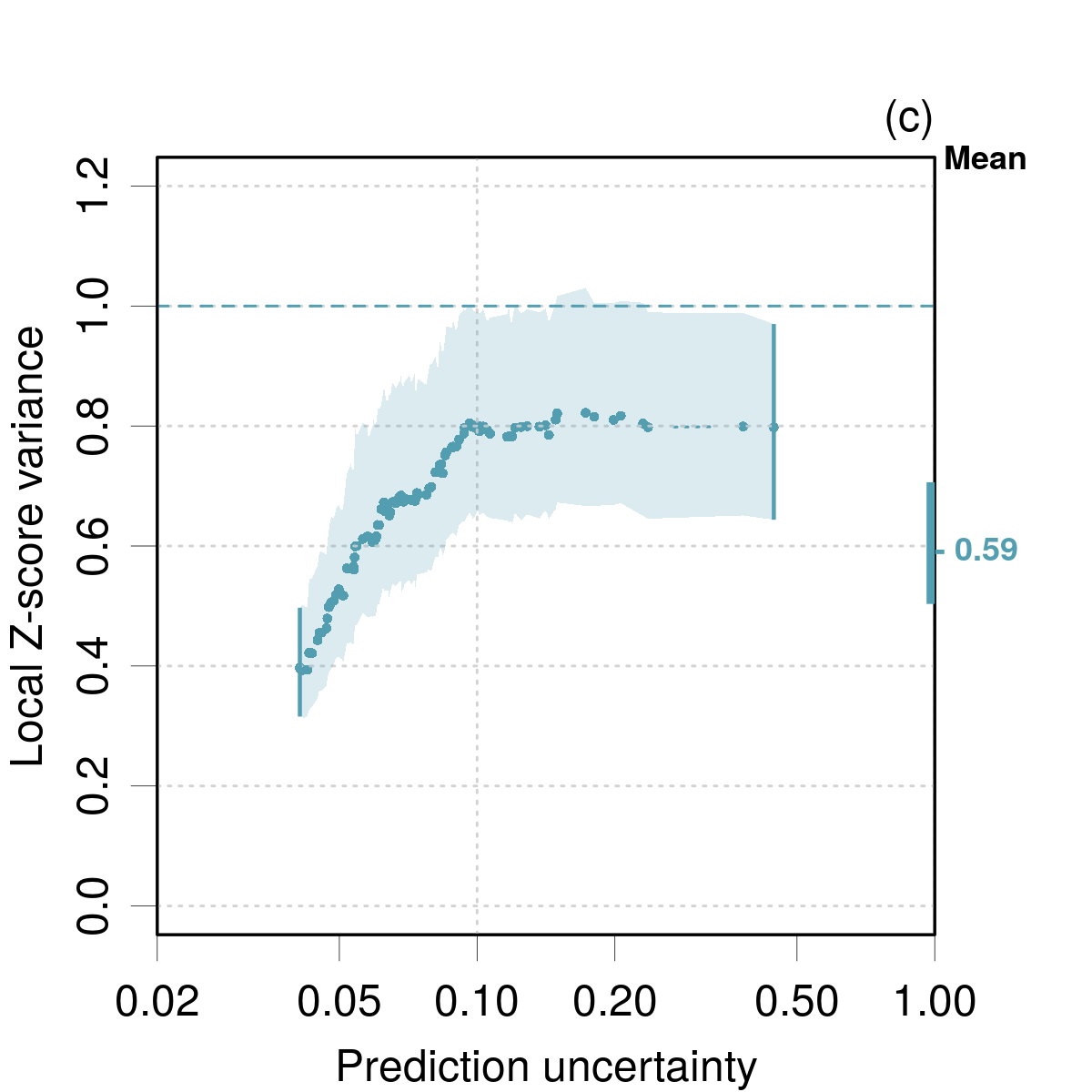
Figure 5: Errors distribution (a) and LZV analysis (b) and (c) for the PRO2021 dataset. (a) and (b) Uniform model dispersion. (c) Polynomial model dispersion.

The PICP is $\nu_{0.95}=0.995(5)$ for both models, i.e., 211 points out of 212 are included in the predicted $I_{95}$ intervals, and the lists of included systems for both models differ only by two points. In such conditions, the coverage statistics cannot be used to differentiate the models, and due to the saturation of the PICP values (very close to the upper limit), the LCP analysis does not provide useful information (not shown).

Considering that the expanded uncertainties were derived by Proppe and Kircher from standard uncertainties by an enlargement factor of 1.96, I derived the standard uncertainties and estimated the $z$-scores statistics. Both sets are unbiased but present variances significantly different from 1: 0.370(43) for model (a) and 0.595(49) for model (b), corresponding to an overestimation of uncertainty. The LZV analysis with a sliding interval of width $M/2$ was performed against prediction uncertainty. The results are shown in Figs. 5(b,c). Three features call for comments: (1) model (b) has a wider range of PUs than model (a), which might help it to better fit the data; (2) model (b) is much closer to the target, notably for small PUs, and (3) both models present a similar trend showing that small PUs are more overestimated than the large ones.

These tests bring evidence that the polynomial model (b) is a notable improvement over the uniform model (a). However there remains a global overestimation of the uncertainties, and the lack of local calibration is not fully resolved.

IV.2 Datasets with standard prediction uncertainty

I consider here datasets where the coverage level of prediction uncertainty is not explicitly provided.

IV.2.1 Standard uncertainty of errors

The most common scenario in the CC-UQ literature is based on standard uncertainties of the predictions and reference data: $V_{i}$, $u_{V,i}$, $R_{i}$ and $u_{R,i}$. The uncertainty on the errors is directly accessible through the combination of variances

$$u_{E,i}=\sqrt{u_{R,i}^{2}+u_{V,i}^{2}}$$ (23)

enabling the computation of $z$-scores without further hypothesis, to be tested by their mean and variance.

Again, non-negligible uncertainties on the reference data might affect the results. If the reference uncertainty is missing, it can be taken as null (for instance in the case of high-accuracy calculated values) or as constant, if a typical value can be found.

IV.2.2 The FEL2008 dataset

This dataset has been extracted manually from Table VII of a 2008 article by D. Feller et al. (Feller2008, ), reporting atomization energies estimated by the FPD method for 106 small molecules. After removing data with missing uncertainty, one is left with a set of 102 systems with a predicted value, a prediction uncertainty, and a reference value with its uncertainty. The prediction and reference uncertainties have to be combined to estimate the errors uncertainty, by a rule that depends on their nature (standard, expanded or other…).

For the reference data, in the absence of specific information, I assumed that expanded uncertainties were used ($U_{95}^{(R)}$). The process of prediction uncertainty estimation in the FPD method has been summarized above (Section II.2.1), and it is difficult to infer its nature, beyond a possible over-estimation implied by the worst-case scenario strategy.

As an initial assessment, I estimated that FPD PUs are close to standard uncertainties and computed $u_{E}$ values as $u_{E,i}=\sqrt{u_{V,i}^{2}+\left(U_{95,i}^{(R)}/1.96\right)^{2}}$and derived the corresponding $z$-scores.

The distribution of errors with their uncertainty is shown in Fig. 6(a). SiH stands as a strong outlier, with an uncertainty too small to cover its large error level. The case is not discussed in the original article, although it is stated that the heat of formation of silicon was not well established at the time of publication. However, there does not seem to be a systematic error, as other Si-containing systems are not visibly affected. Other outliers such as BN or B₂ have error bars large enough to cover their deviation.

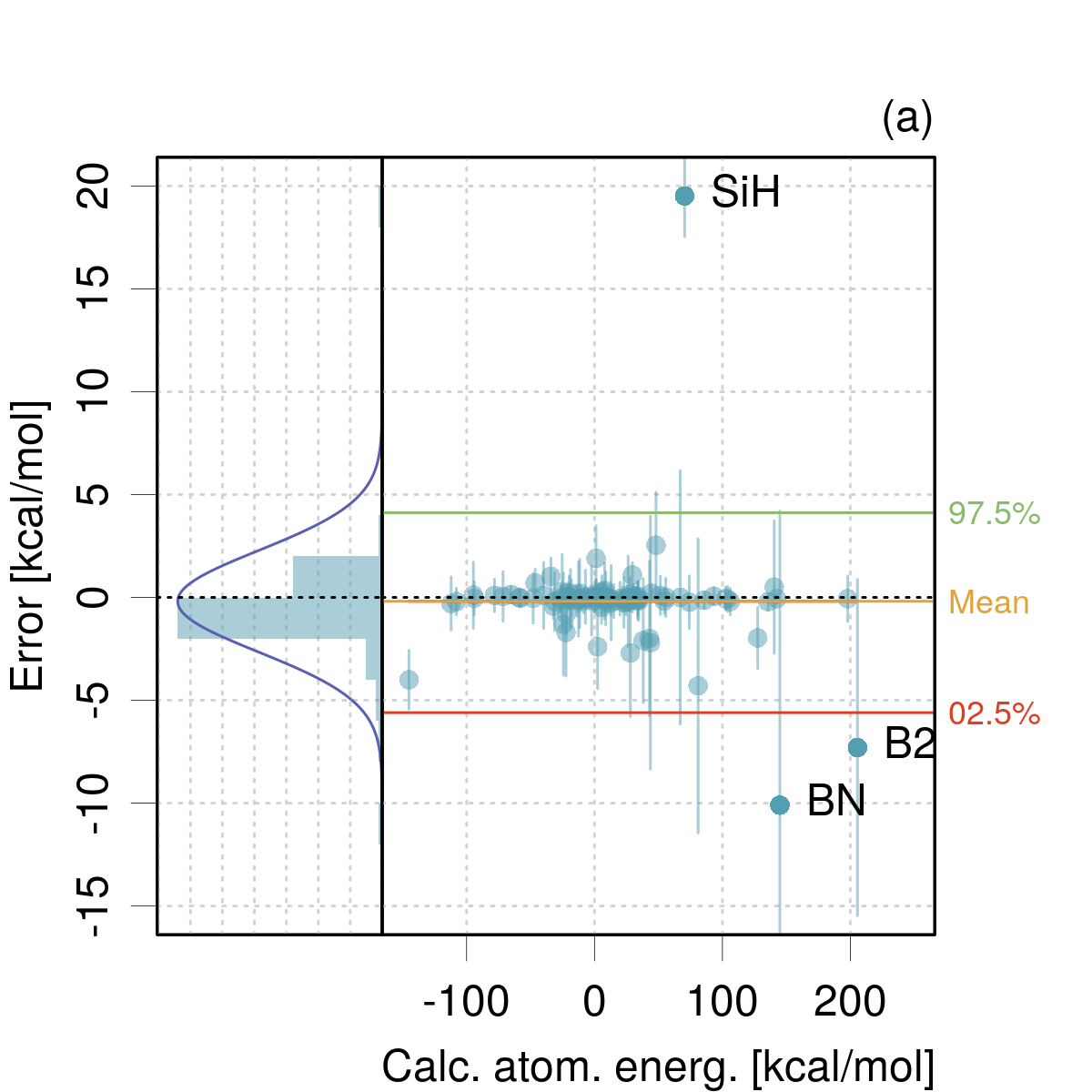
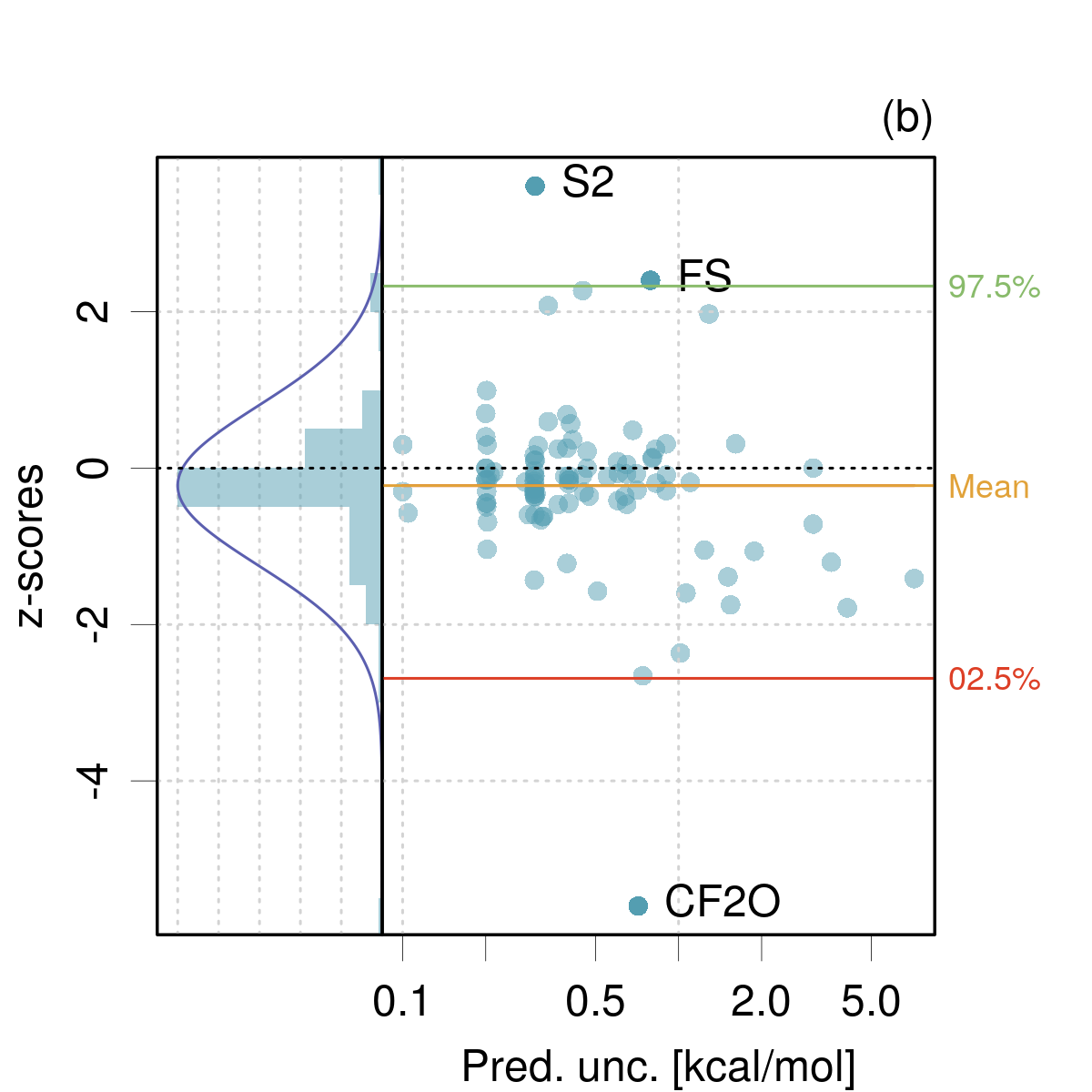
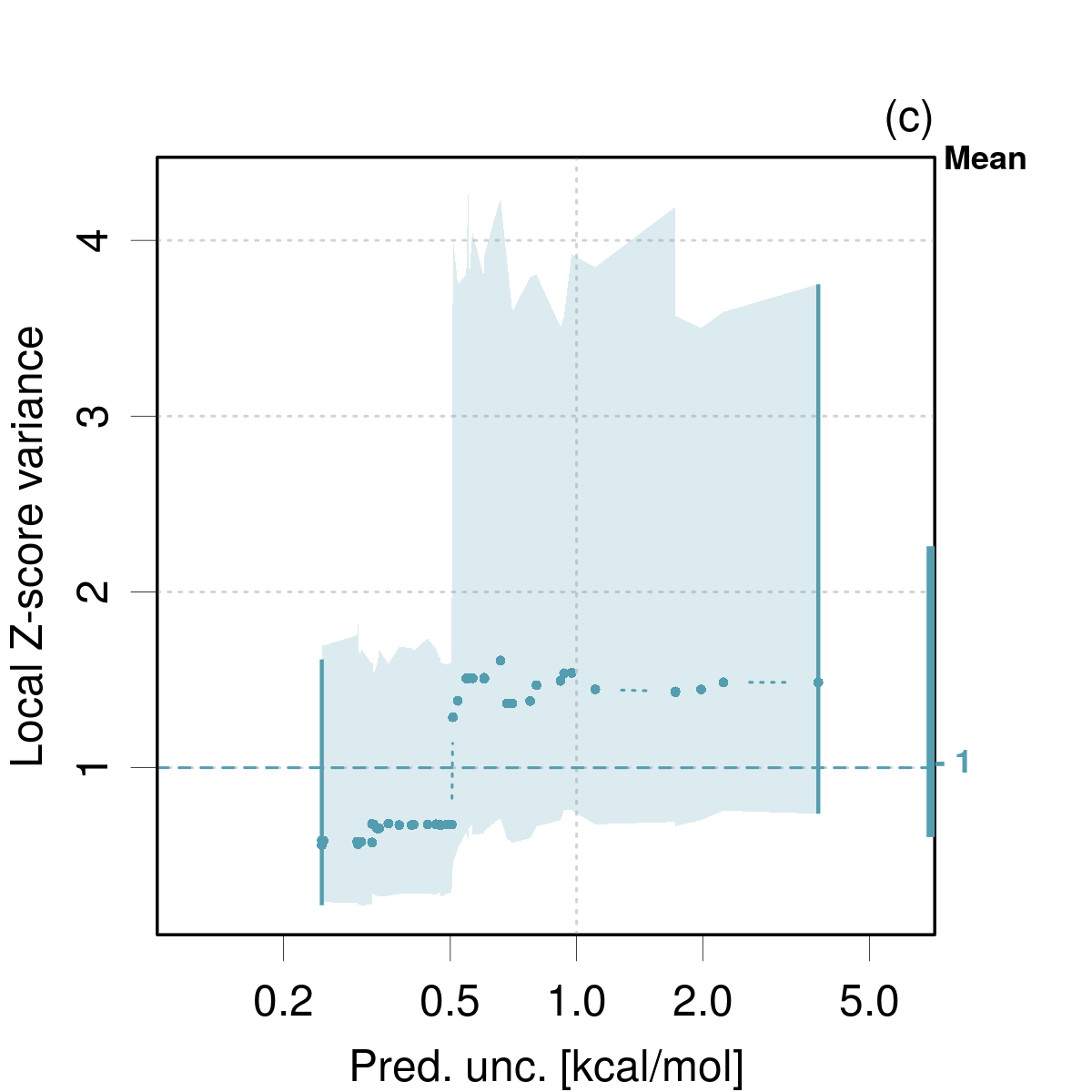
Figure 6: Distribution of errors (a), z-scores (b) and LZV analysis (c) for the FEL2008 dataset. In (a) and (b), the left panel shows an histogram of the data with its best amplitude-normalized Gaussian fit. The SiH system has been removed for the $z$-score plot and LZV analysis.

A plot of the $z$-score distribution after the removal of the SiH system (Fig. 6(b)) reveals two points with outstanding values: the atomization energies of S₂ and CF₂O have apparently underestimated uncertainties. The histogram of the $z$-scores (Fig. 6(b), left panel) shows a strong concentration of small $z$-scores values and a strong departure from a normal shape. Nevertheless, the variance of the $z$-scores is close to 1: $\mathrm{Var}(Z)=1.04(33)$, which does not invalidate the derivation of $u_{E}$. The LZV analysis against prediction uncertainty is shown in Fig. 6(c) for a sliding window of width $M/2$, showing no significant deviation from the target, considering the large uncertainties. There is a slight positive trend, with a step around 0.5 kcal/mol, which is linked to the prevalence of negative $z$-score values for larger PUs (Fig. 6(b)).

Unless my treatment of the original data is unduly lucky, it appears that the “crude and hopefully conservative” appreciation of the original authors (Feller2017, ) might be self-deprecating, but more data would be necessary to conclude.

IV.2.3 The PAN2015 dataset

A dataset of 257 formation heats predicted by the mBEEF method, and their standard uncertainties, have been extracted from a 2015 article Pandey and Jacobsen (Pandey2015, ). The reference data have no uncertainty reported. I previously analyzed this dataset (PAN2015) (Pernot2017b, ), showing an inconsistency between the prediction uncertainties and the errors amplitudes. For instance, the mean prediction uncertainty (Eq. 7; 0.18 kcal/mol) significantly exceeds the standard deviation of the errors ($\mathrm{sd}(E)=0.13$ kcal/mol). I propose here to check how the proposed validation methods perform with this dataset.

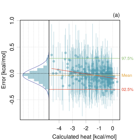
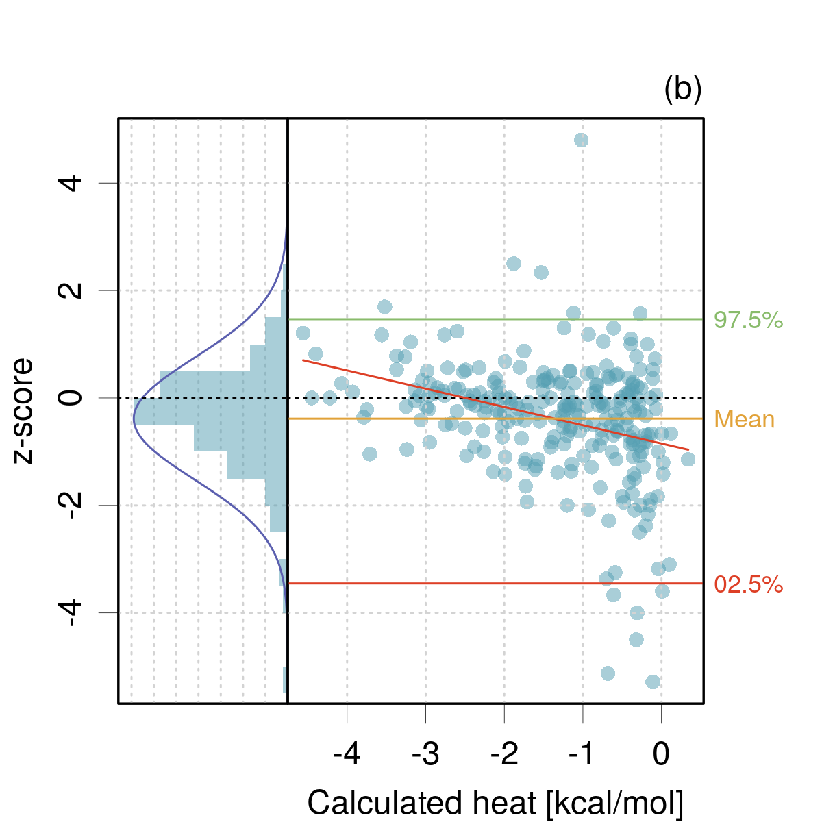
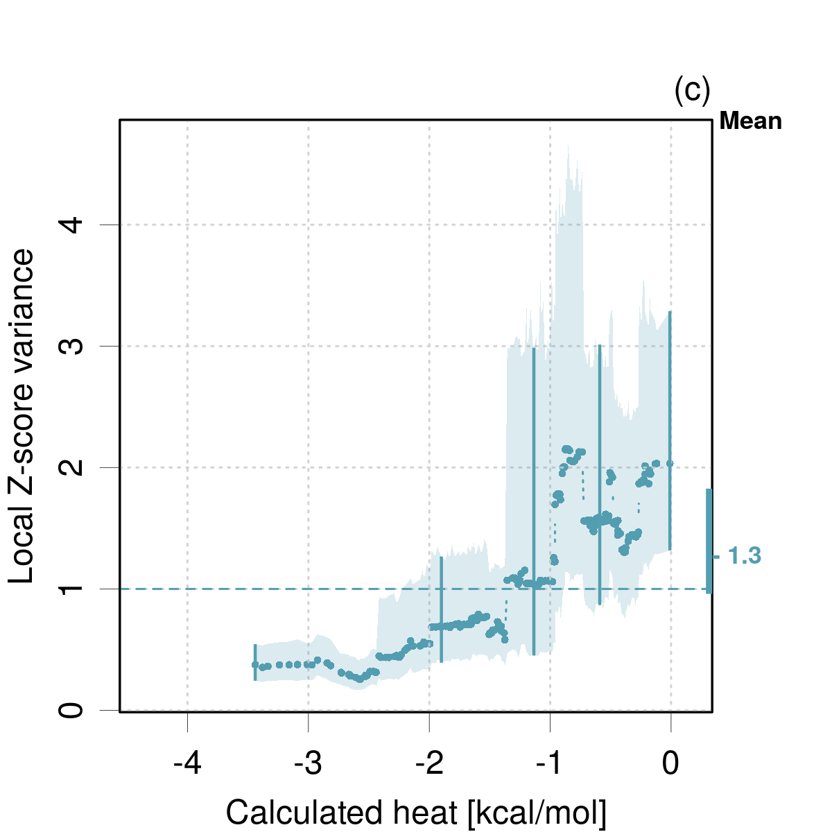
Figure 7: Distribution of errors (a) and $z$-scores (b) for the PAN2015 dataset. LZV analysis of $z$-scores along the predicted values (c) and the predicted uncertainties (d), using a sliding window of width $M/5$.

The error set and the corresponding $z$-scores are plotted in Fig. 7. Both distributions deviate from normality. Besides a small trend in both quantities, the main feature in these plots is the heterogeneity of the $z$-scores distribution along the predicted values, with a noticeable negative tail for heats above -1 kcal/mol. Some uncertainties in this area seem to be underestimated.

The global $z$-scores statistics are not ideal: $\mathrm{E}(Z)=-0.385(72)$ and $\mathrm{Var}(Z)=1.28(20)$ with a 95 % confidence interval $[0.96,\thinspace 1.80]$. The variance is not incompatible with its target (1), but considering the heteroscedasticity of the $z$-scores, it increases from about 0.5 for the first half of the dataset to about 2 for the second half, with confidence intervals excluding 1 (LZV analysis, Fig. 7(c)). The LZV analysis with respect to the prediction uncertainty shows the opposite trend, decreasing from a value above 3 to about 0.5 for the larger PUs (Fig. 7(d)). Briefly, small uncertainties are underestimated, while large ones are overestimated.

IV.2.4 The PAR2019 dataset

A dataset of 35 harmonic vibrational frequencies (PAR2019) has been extracted from an article by Parks et al. (Parks2019, ) (Table I, columns $\mu$ and $\sigma$), as another example of BEEF-generated uncertainties. This is a small dataset, which puts the validation methods to their limits. The errors are plotted in Fig. 8(a), and the corresponding $z$-scores are plotted in Fig. 8(b).

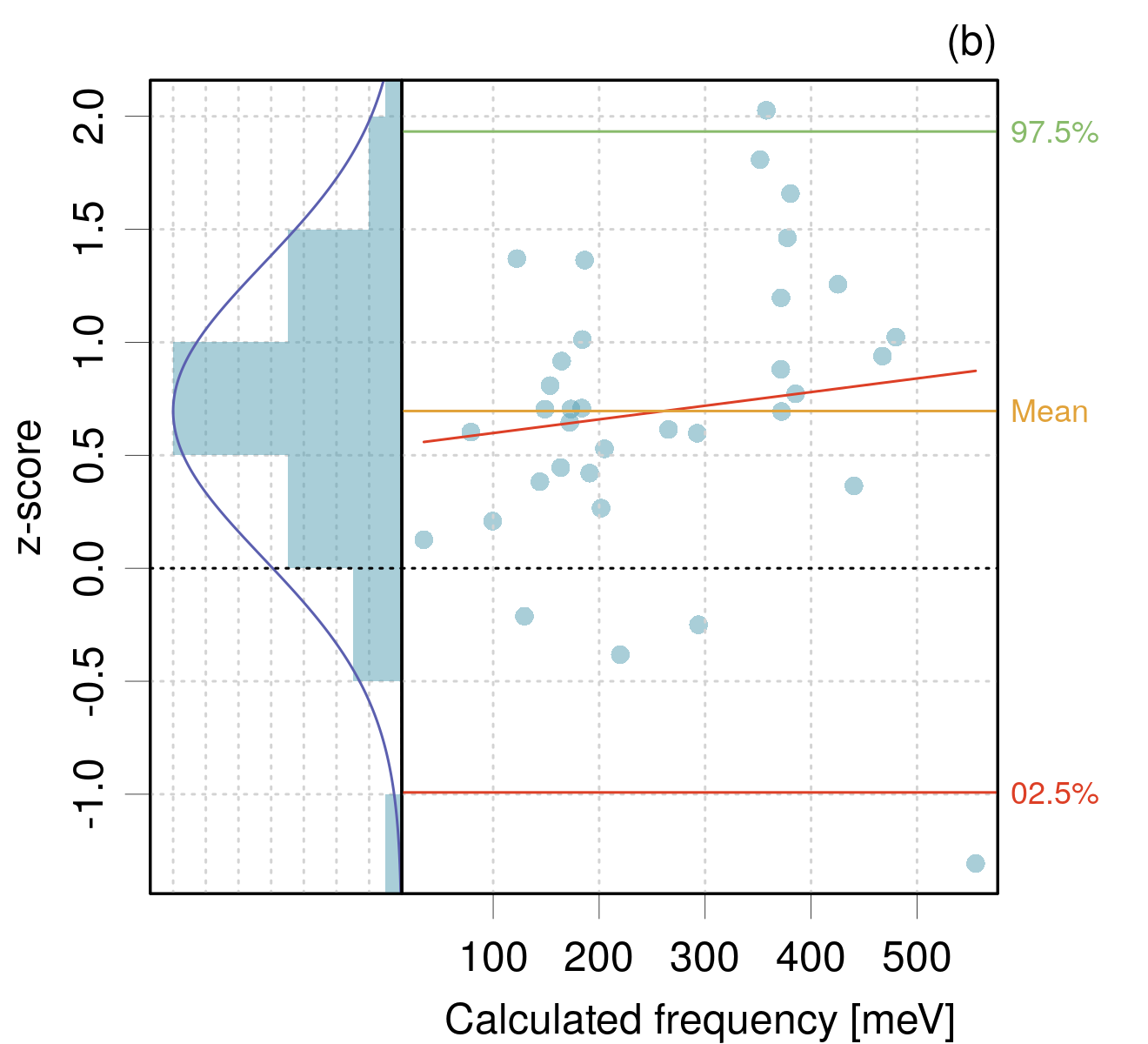
Figure 8: Distribution of errors (a) and $z$-scores (b) for the PAR2019 dataset.

In Fig. 8(a), many error bars appear too large with respect to the error amplitudes and there is a non-negligible bias. The $z$-scores are also notably biased, while their variance is 0.42(13) with a 95 % confidence interval of $\left[0.23,\thinspace 0.81\right]$, excluding the target value. The data are too sparse to attempt a LZV analysis.

BEEF-based CC-UQ methods seem to enjoy some popularity, but we saw on two examples that they have to be used with care. Pernot and Cailliez (Pernot2017, ) showed that the capture of model errors into the variance-covariance matrix of a model’s parameters (or into their Bayesian posterior pdf) might be problematic. As the calibration is quantified by the mean prediction variance, there is no guarantee that the prediction uncertainty is reliable for any single prediction. In fact, this parameters uncertainty inflation (PUI) scheme (Pernot2017b, ) implies strong functional constraints which play against its local calibration (Simm2016, ; Reiher2022, ).

IV.3 A-posteriori UQ methods

A-posteriori prediction uncertainty has to be estimated by a statistical model using the differences between model predictions and reference data, and complementary uncertainty information, when available. The main target is to provide reliable prediction uncertainty in the shape of standard and/or expanded uncertainty.

The first step in prediction uncertainty estimation is the correction of trends in the errors dataset. The estimation of trends typically relies on the calculated value, $V$, as a predictor variable (Pernot2011, ; Lejaeghere2014, ; Pernot2015, ; Proppe2017, ), but more complex scenarios can be considered, as might be done in QSAR (Cronin2019, ) and ML (Tran2020, ; Venkatraman2021, ) methods.

The workhorse model of trend correction is the low-degree polynomial. I note below PTC$n$ (Polynomial Trend Correction of order $n)$ the correction of the error trend vs. $V$ by a polynomial of degree $n$. For this study, the PTC$n$ model’s parameters and their uncertainty are estimated by standard least-squares, which is known to be robust to non-normal error distributions (Knief2021, ). More complex prediction uncertainty models could be used for datasets presenting complex trends, requiring weighting schemes (e.g., in the case of heterogeneous reference values uncertainties (Pernot2015, )) or the consideration of heteroscedasticity (Bakowies2021, ; Proppe2021, ). More specific trend correction models are defined in their application case. Once trends have been corrected, one is left with a set of residual errors which can be considered as unpredictable and can be treated as random variables.

I have considered in this study three methods (DIST, PRED and EQ) to estimate either prediction uncertainty or the limits of 100$p$ % prediction intervals. All these methods assume the homoscedasticity of the errors:

• DIST: based on mean and standard deviation of the error set that provide a standard uncertainty,

  $$\mu =\mathrm{mean}(E)$$ (24)

  $$u_{E} =\mathrm{sd}(E)$$ (25)

  The interest of this model is to enable the user to infer a prediction uncertainty from statistics often reported in benchmark tables. Note that for well corrected trends, one should have $\mu\simeq 0$. In order to avoid hypotheses on the errors distribution, the use of $z$-scores based validation methods is best suited to this case. Note that, by construction, one will get $\mathrm{Var}(Z)=1$, and the focus should be on the sharpness assessment by LZV analysis.

• PRED: based on the least-squares based statistical predictions of the trend correction model (Pernot2015, ; DeWaele2016, ; Proppe2017, ). The least-squares formalism provides standard prediction uncertainty or expanded uncertainty at any probability level. The prediction intervals account for the parametric uncertainty of the correction polynomial, but are symmetrical and derive from the expansion of the prediction uncertainty by Student’s-$t$ factors. This approach can be validated by PICP-based and $z$-score-based methods.

• EQ: based on empirical quantiles $q_{p}$ estimated from the errors set. This model makes no distribution hypothesis, except that the errors empirical cumulative distribution function is a good proxy for the CDF of prediction errors $F$. It ignores the parametric uncertainty due to the trend correction model, but it enables to treat non-normal errors distributions and to estimate 100$p$ % prediction intervals from quantiles of the errors distribution

  $$I_{p} =\left[q_{(1-p)/2}(E),q_{(1+p)/2}(E)\right]$$ (26)

  This approach guarantees a good average calibration, but not local calibration, as the global distribution might not be locally optimal in the presence of heteroscedasticity. The EQ method can be validated by the full arsenal based on PICP estimation. A symmetrized expanded uncertainty, noted SEQ_p can be defined as the half range of $I_{p}$.

Cross-validation.

For a-posteriori methods, one can benefit from the ability to estimate a prediction uncertainty repeatedly to enrich the LCP analysis with cross-validation. Schematically, one proceeds as follows:

1. Cross-validation (repeat until all points are tested)

   1. Split randomly the data into learning and test sets.

   2. Use the learning set to estimate prediction intervals.

   3. Test these intervals on the test set (Does the interval contain the test value or not ?).

2. Dispatch the test results into the chosen areas of the predictor variable, and estimate the PICPs as the percentage of positive tests in each interval $\nu_{i}$.

Leave-One-Out (LOO) or k-fold cross-validation can be used in step 1. To improve the estimation of $\nu$, k-fold cross-validation can also be repeated several times on randomly reordered datasets.

IV.3.1 The PER2017 dataset

The most famous a-posteriori method might be the scaling of harmonic frequencies. A few years ago, I showed that it had the notable interest to enable the estimation of a prediction uncertainty (Pernot2017b, ). As an example, I used a set of 2278 frequencies calculated at the CCD/6-31G* level, extracted from the CCCBDB (cccbdb_6_1, ). To check calibration, I then estimated the 2-$\sigma$ PICP, which ideally was 95 %, and much better than for a concurrent method. I propose here to revisit this dataset.

The distribution of errors after scaling is presented in Fig. 9(a), from which one can make two observations: (1) in the absence of the constant term in the correction model, the scaling does not fully correct the bias (there is still a very small trend in the errors, which is probably irrelevant); and (2) the histogram is far from being normal. More problematic, the dispersion of the errors does not seem to be uniform along the predictor axis. One might thus expect less than optimal local calibration.

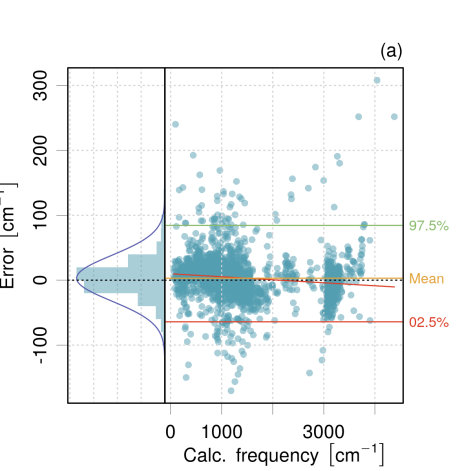
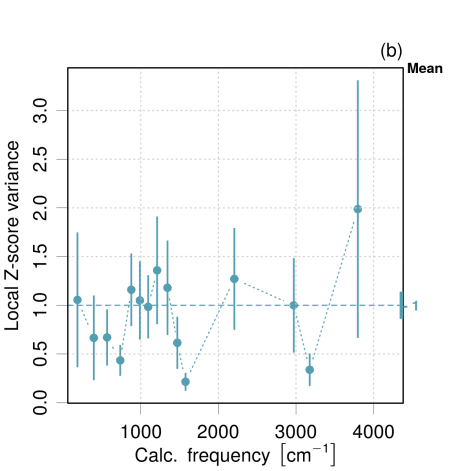
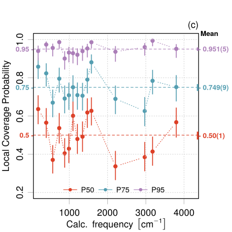
Figure 9: (a) Distribution of errors after scaling of harmonic frequencies obtained at the CCD/6-31G* level of theory (set PER2017); (b) LZV analysis; and (c) LCP analysis of PICPs estimated by the EQ method.

Let us consider first the $z$-scores analysis with a prediction uncertainty derived by the DIST approach (Fig. 9(b)). By construction, the variance of the $z$-scores is 1, but the LZV analysis reveals a local calibration issue, with several areas with small variance values deviating significantly from the target.

Not surprisingly, considering the shape of the errors distribution in Fig. 9(a), the PICP values returned by the PRED approach are off, 0.70(1) vs 0.50 and 0.864(7) vs 0.75, except at the 0.95 level, where the PICP is 0.944(5). The latter value was the one I used to validate the prediction uncertainty estimation in my earlier study.

A much better calibration is automatically obtained by using prediction intervals based on the EQ approach (Fig. 9(c)), but the issue of sharpness becomes prominent, as some local PICP values deviate significantly from their targets. Note however that the situation is not so bad at the 0.95 level, and one would still get a reasonable estimation of a uniform $U_{95}$ value (70 cm^-1) depending on the intended application.

Nevertheless, this questions the reliability of the prediction uncertainty derived by the scaling procedure for this dataset, which features multiple underlying trends. More elaborate, bond-based, scaling methods (Pulay1979, ; Legler2015, ) might enable to derive better predictions.

IV.3.2 The PAN2015 dataset: An alternative view

For comparison with the original prediction uncertainty estimation, I applied an a-posteriori analysis to the PAN2015 dataset analyzed above (Sections IV.2.3). Considering the trend observed in the errors, I used a linear trend correction (PTC1). The distribution of residual errors is shown in Fig. 10(a). The distribution is still not perfectly normal.

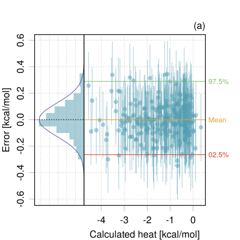
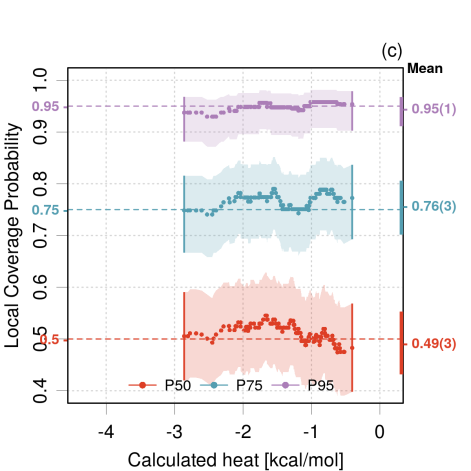
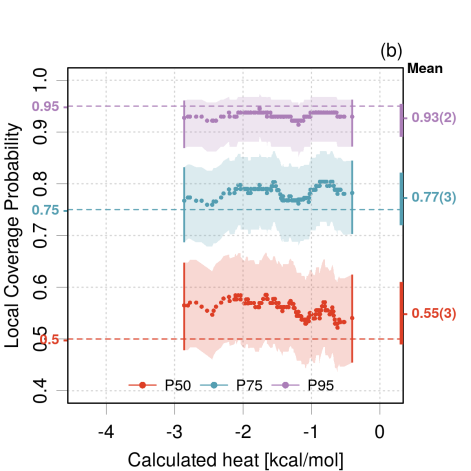
Figure 10: Distribution of errors (a) and LCP analysis for an a-posteriori reanalysis of the PAN2015 errors with a PTC1 correction and PRED model (b) or EQ model (c).

Using the PRED method, the PICP values 0.55(3)/0.77(3)/0.93(2) are nevertheless consistent with their targets Fig. 10(b). Although the LCP analysis does not provide evidence of local calibration issues, there seems to be a small systematic bias on the local PICP values that could be compensated for by using the EQ approach Fig. 10(c).

The mean prediction uncertainty estimated by the PRED model is about 0.13 kcal/mol. By comparison, the BEEF-based PUs range from 1/4th to 3 times this value, with about 67 % of them in excess.

IV.3.3 ML and $\Delta$-ML datasets

The data are issued from a study by Zaspel et al. (Zaspel2019, ), as used and analyzed by Pernot et al. (Pernot2020b, ). They contain the effective atomization energies (EAEs) for the QM7b dataset (Montavon2013, ), for molecules up to seven heavy atoms (C, N, O, S or Cl). I consider here values for the cc-pVDZ basis set, the MP2 and CCSD(T) ab initio methods, and two machine learning algorithms (CM-L1 and SLATM-L2). The ML methods have been trained over a random sample of 1000 CCSD(T) energies completed by a set of 350 outliers for the SLATM-L2 method identified by Pernot et al. (Pernot2020b, ). The final dataset for this study contains the prediction errors for the 5861 remaining systems by the MP2 and SLATM-L2 methods. In complement to the previous data, the errors of MP2 with respect to CCSD(T) have been learned by the CM-L1 and SLATM-L2 methods, providing new $\Delta$-ML/CM-L1 and $\Delta$-ML/SLATM-L2 datasets (unpublished, kindly provided by B. Huang).

It has been observed previously that the MP2 errors have a quasi-normal distribution, which was not the case for the SLATM-L2 dataset. Assuming a normal CDF of prediction errors through the use of a PTC1/PRED scenario, I built calibration curves to illustrate their diagnostic features. Note that, considering the large number of points, the parametric uncertainty for the linear correction is negligible, and one is basically testing here the normality of the corrected error sets. The plots in Fig. 11, confirm the calibration for MP2 PUs, while the notable heavy tails of the SLATM-L2 errors do not benefit from a trend correction, leading to a distorted calibration curve. The $\Delta$-ML/CM-L1 dataset presents a slight distortion of the calibration curve. In contrast, the $\Delta$-ML/SLATM-L2 dataset (not shown) presents the same profile as SLATM-L2. Considering the MisCal statistic, the MP2/PTC1/PRED and $\Delta$-ML/CM-L1/PTC1/PRED methods are validated, but MP2/PTC1/PRED is the one with the smallest calibration error (CalErr = 0.028).

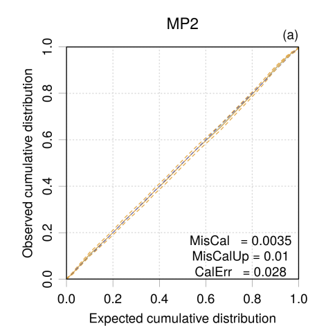
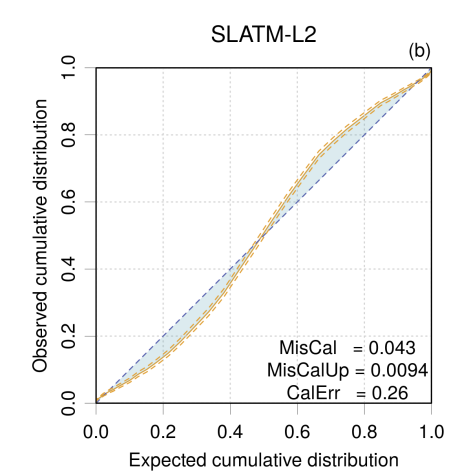
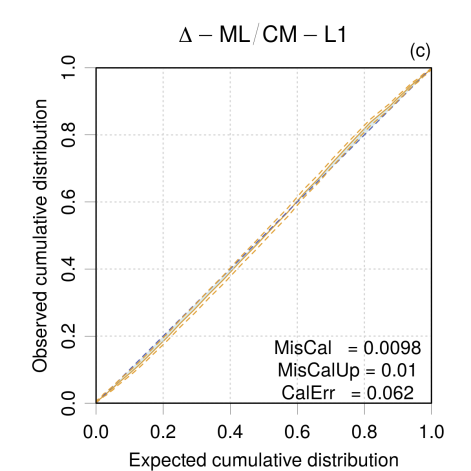
Figure 11: Calibration curves for the prediction uncertainty of effective atomization energies by (a) MP2, (b) SLATM-L2 and (c) $\Delta$-ML/CM-L1 methods with a PTC1/PRED calibration scenario.

The PTC1/PRED method provides us with standard PUs and confidence intervals. Their sharpness can be tested by LZV and LCP analysis, respectively. The LZV plots are presented in Fig. 12, and the LCP plots are given in Fig. 13.

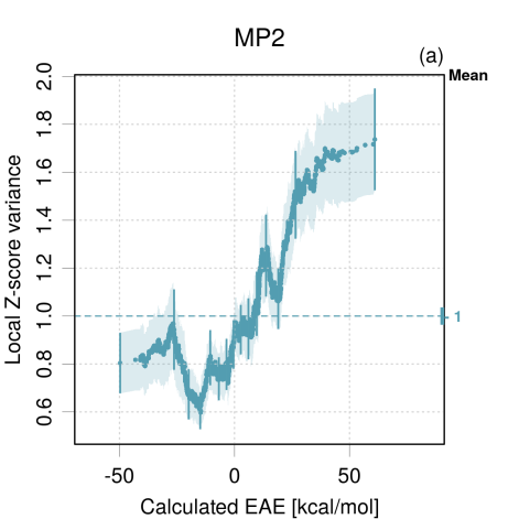
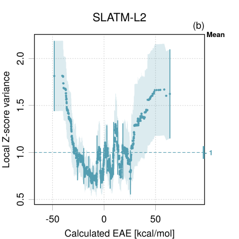
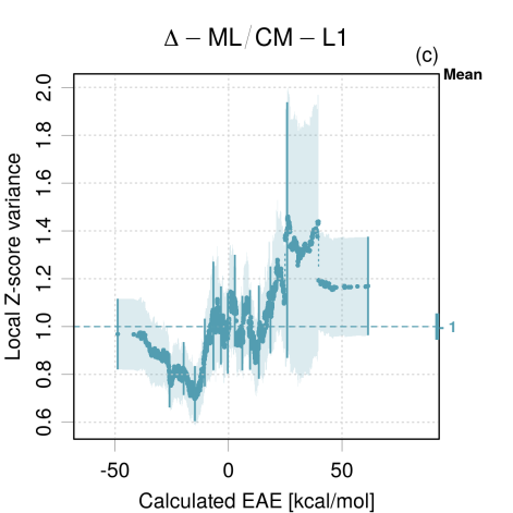
Figure 12: LZV analysis for the prediction uncertainty of effective atomization energies (EAEs) by (a) MP2, (b) SLATM-L2 and (c) $\Delta$-ML/CM-L1 methods with a PTC1/PRED calibration scenario.

The uniform standard prediction uncertainty estimated by the PTC1/PRED method seems to have severe local calibration issues, notably for MP2 and SLATM-L2 (Fig. 12). For MP2, the prediction uncertainty overestimates the dispersion of the errors for negative energies, while it underestimates it for the positive ones. For SLATM-L2, the underestimation occurs a both extremities. The situation is better for $\Delta$-ML/CM-L1, which deviates significantly from the target for small negative values. A similar dip in the $z$-score variance is visible for the other methods, which might correspond to a set of molecules for which the CCSD(T) energies are more closely approximated by all three methods. We can consider that the prediction uncertainty extracted from $\Delta$-ML/CM-L1 is rather reliable. Note that its largest significant deviation of $\mathrm{Var}(Z)$ (about 0.8) corresponds to a local excess of about 10 % on the prediction uncertainty ($1/\sqrt{0.8}\simeq 1.1$). By comparison, the largest variance deviation for MP2 (about 1.7) corresponds to an underestimation of the local prediction uncertainty by a factor $1/\sqrt{1.7}\simeq 2.6$.

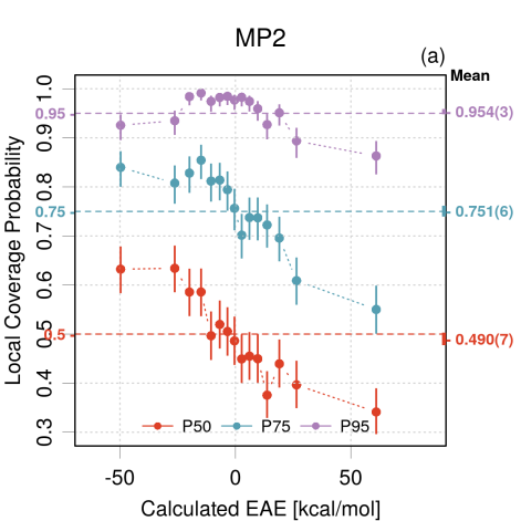
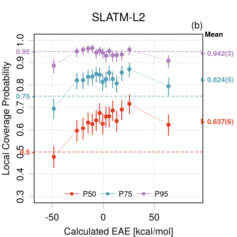
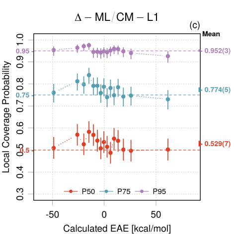
Figure 13: LCP analysis for the prediction uncertainty of effective atomization energies (EAEs) by (a) MP2, (b) SLATM-L2 and (c) $\Delta$-ML/CM-L1 methods with PTC1/PRED calibration scenario.

The PRED method also enables to generate prediction intervals for a LCP analysis. Local calibration of the PCT1/PRED scenario is evaluated in Fig. 13. One sees that despite its quasi-normal errors distribution and good calibration statistics, MP2 presents a sharpness problem at all coverage levels (Fig. 13(a)). At the 0.5 and 0.75 levels, the LCP curves confirm the observations made through the LZV analysis (prediction uncertainty overestimation for the negative energy values and underestimation for the positive ones). This effect is partially lost at the 0.95 level. For SLATM-L2 (Fig. 13(b)), the poor calibration of the PRED intervals is clearly visible, notably at the 0.5 and 0.75 levels, and local calibration problems are also detected, notably at the smaller coverage probabilities. Using a quantile-based method (EQ) would improve average calibration but not locally. In the $\Delta$-ML/CM-L1 case (Fig. 13(c)) calibration is globally very good, but one still observes a deviation for the small negative energy values, as seen in the LZV analysis.

Considering the acceptable-to-good local calibration of the ML methods at the 95 % level, one can consider the possibility to define a uniform prediction uncertainty. Table 1 reports the values of the bias (mean error), 95 % prediction intervals ($I_{95}$), prediction uncertainty ($u_{p}$, estimated as the standard deviation of the errors), expanded prediction uncertainty ($U_{95}$, as the half range of $I_{95}$), and expansion factor $(f_{95}=U_{95}/u_{p})$. MP2 is added for comparison although it is not well calibrated enough to provide reliable uncertainty statistics.

Method	Bias		$I_{95}$		$u_{p}$		$U_{95}$		$f_{95}$
	(kcal/mol)		(kcal/mol)		(kcal/mol)		(kcal/mol)
MP2	-0.	04(2)	[-3.	39(6), 2.84(8)]	1.	61(2)	3.	12(5)	1.	94(2)
SLATM-L2	0.	05(2)	[-2.	37(7), 2.63(8)]	1.	20(2)	2.	50(5)	2.	08(3)
$\Delta$-ML/SLATM-L2	0.	003(2)	[-0.	35(1), 0.32(1)]	0.	169(3)	0.	336(7)	1.	99(3)
$\Delta$-ML/CM-L1	0.	03(1)	[-1.	49(3), 1.50(3)]	0.	77(1)	1.	49(2)	1.	93(2)

Table 1: Bias and prediction uncertainties for effective atomization energies by MP2 and ML methods.

The bias is negligible in all cases, smaller or equal to the uncertainty on the limits of $I_{95}$. For simplicity, the other statistics have been obtained without correction of the error sets. The $I_{95}$ limits present a good symmetry, with a slight defect for MP2 and SLATM-L2. The LCP analysis showed that $U_{95}$ provides a prediction interval with a reliable 95 % coverage for all ML methods, except for extreme energy values for SLATM-L2 and $\Delta$-ML/SLATM-L2. As the errors distributions are not normal in these cases, one should also provide a standard prediction uncertainty for further uncertainty propagation. It is remarkable that the expansion factor between $u_{p}$ and $U_{95}$ is close to the value expected for a normal distribution (1.96). The largest difference is for SLATM-L2, with $f_{95}=2.08(3)$. For all practical purposes, a factor two might be acceptable. As a byproduct of this analysis, one can note the excellent performance of the $\Delta$-ML/SLATM-L2 method to predict CCSD(T) values, with a prediction uncertainty of 0.17 kcal/mol, about 1/10th of the MP2 error standard deviation, albeit with large local calibration problems.

In a recent article comparing MP2 (normal error distribution) with SLATM-L2 (non-normal) (Pernot2020b, ), the authors argued that the former would probably be a wiser choice for reliable predictions. This suggestion does not stand against the present results, as MP2 is worse than SLATM-L2 at the LCP test. In fact, it would even be reasonable to use SLATM-L2 to define a constant expanded uncertainty $U_{95}$, which is not the case for MP2.

V Conclusion

The use of computational chemistry in practical applications is a strong incentive to establish levels of confidence on the calculated properties. In this paper, I considered the concepts of calibration and sharpness, and the associated metrics and graphical checks, developed for probabilistic forecasters, notably in meteorology and more recently in machine learning. I adapted these methods to computational chemistry uncertainty quantification scenarios and I applied them to a series of datasets covering both embedded and a-posteriori CC-UQ methods.

The validation methods were adapted to the level of available information, notably to avoid uncontrolled hypotheses on the error distributions. In particular, while the calibration of expanded uncertainties can be directly tested using prediction interval coverage probabilities (PICP), validation of prediction uncertainty sets was based on the analysis of $z$-scores variance. Instead of sharpness assessment, I focused here on local calibration along a predictor quantity, leading to local versions of the PICP (LCP analysis) and $z$-scores variance (LZV analysis) tests, which proved to be very convenient and useful in our context.

The main conclusions arising from the application cases are the following:

1. Calibration validation should preferably be performed by the UQ providers. There is a formidable loss of information when summarizing UQ to prediction uncertainty. Validation of prediction uncertainty is strongly dependent on the hypothesis of errors distributions. We met several instances where uncertainties reported in the literature had ambiguous meanings. They might be standard or expanded uncertainties or provide only a part of the error budget, for instance the variability of stochastic systems (Bergmann2020, ; Lin2021, ).

2. Establishing reliable PUs is not an easy task. In fact, very few of the considered examples provide acceptable levels of average and local calibration. The most satisfying example was provided by a $\Delta$-ML method, which is in line with observations by Tran et al. (Tran2020, ) who observe that “methods that use one model to make value predictions and then a subsequent model to make uncertainty estimates were more calibrated than models that attempted to make value and uncertainty predictions simultaneously”. We saw that a-posteriori methods can be used to ensure average calibration, however, they cannot always provide local calibration.

3. The sample sizes required to test confidently either PICP values or $z$-scores variances often exceed the size of computational chemistry benchmark datasets. This is even more limiting when testing local calibration. In such cases, the trend in curves of the LCP/LZV analysis provide an interesting diagnostic, even when statistical uncertainties are large.

4. Reliably testing PICP or variance values requires some care, as the standard tests often make hypotheses on the sample distribution which are not met by computational chemistry errors.

5. Considering that most prediction uncertainty estimates analyzed in this study were rejected on the basis of rigorous statistical criteria, one might want to loosen the acceptance thresholds. The pending question is thus how much of miscalibration is acceptable for specific applications. The community has to seize this problem.

6. One has always to keep in mind that error statistics are affected by the quality of reference data. In the present validation framework, an additional factor to consider is the quality of reference data uncertainty. In the limit of perfect correction of model predictions, and therefore of tiny prediction uncertainty, reference data uncertainty would become the main contribution to, and subject of, calibration statistics.

I hope that the concepts and tools presented here will enable a unified and more rigorous testing framework for my colleagues interested in virtual measurements and more generally in prediction uncertainty of computational chemistry methods.

Data availability statement

The data and codes that enable to reproduce the figures and tables of this study are openly available at the following URL: https://github.com/ppernot/PU2022, or in Zenodo at https://doi.org/10.5281/zenodo.5818026.

Supplementary Material

See supplementary material for details on PICP testing, $z$-scores variance testing and an atlas of calibration checks.

References

- (1) K. Lejaeghere. The uncertainty pyramid for electronic-structure methods. In Y. Wang and D. L. McDowell, editors, Uncertainty Quantification in Multiscale Materials Modeling, Elsevier Series in Mechanics of Advanced Materials, pages 41 – 76. Woodhead Publishing, 2020.
- (2) J. B. Rommel. From Prescriptive to Predictive: an Interdisciplinary Perspective on the Future of Computational Chemistry. arXiv:2103.02933 [physics], 2021. URL: http://arxiv.org/abs/2103.02933.
- (3) M. Reiher. Molecule-specific uncertainty quantification in quantum chemical studies. Israel Journal of Chemistry, 62(1-2):e202100101, 2022.
- (4) J. Wellendorff, K. T. Lundgaard, K. W. Jacobsen, and T. Bligaard. mBEEF: An accurate semi-local bayesian error estimation density functional. J. Chem. Phys., 140:144107, 2014.
- (5) B. Ruscic. Uncertainty quantification in thermochemistry, benchmarking electronic structure computations, and active thermochemical tables. Int. J. Quantum Chem., 114:1097–1101, 2014.
- (6) P. Pernot, B. Civalleri, D. Presti, and A. Savin. Prediction uncertainty of density functional approximations for properties of crystals with cubic symmetry. J. Phys. Chem. A, 119:5288–5304, 2015.
- (7) P. Pernot and A. Savin. Probabilistic performance estimators for computational chemistry methods: the empirical cumulative distribution function of absolute errors. J. Chem. Phys., 148:241707, 2018.
- (8) K. K. Irikura, R. D. Johnson, and R. N. Kacker. Uncertainty associated with virtual measurements from computational quantum chemistry models. Metrologia, 41:369–375, 2004.
- (9) S. Wan, R. C. Sinclair, and P. V. Coveney. Uncertainty quantification in classical molecular dynamics. Phil. Trans. R. Soc. A, 379:20200082, 2021.
- (10) J. J. Gabriel, N. H. Paulson, T. C. Duong, F. Tavazza, C. A. Becker, S. Chaudhuri, and M. Stan. Uncertainty Quantification in Atomistic Modeling of Metals and Its Effect on Mesoscale and Continuum Modeling: A Review. JOM, 73:149–163, 2021.
- (11) Y. Mao, A. Gerisch, J. Lang, M. C. Böhm, and F. Müller-Plathe. Uncertainty Quantification Guided Parameter Selection in a Fully Coupled Molecular Dynamics-Finite Element Model of the Mechanical Behavior of Polymers. J. Chem. Theory Comput., 17:3760–3771, 2021.
- (12) D. Ye, L. Veen, A. Nikishova, J. Lakhlili, W. Edeling, O. O. Luk, V. V. Krzhizhanovskaya, and A. G. Hoekstra. Uncertainty quantification patterns for multiscale models. Phil. Trans. R. Soc. A, 379:20200072, 2021.
- (13) J. Proppe, T. Husch, G. N. Simm, and M. Reiher. Uncertainty quantification for quantum chemical models of complex reaction networks. Faraday Discuss., 195:497–520, 2016.
- (14) G. N. Simm and M. Reiher. Systematic Error Estimation for Chemical Reaction Energies. J. Chem. Theory Comput., 12:2762–2773, 2016.
- (15) B. Hie, B. D. Bryson, and B. Berger. Leveraging uncertainty in machine learning accelerates biological discovery and design. Cell Systems, 11:461–477.e9, 2020.
- (16) V. Volodina and P. Challenor. The importance of uncertainty quantification in model reproducibility. Phil. Trans. R. Soc. A, 379:20200071, 2021.
- (17) D. Feller, K. A. Peterson, and D. A. Dixon. A survey of factors contributing to accurate theoretical predictions of atomization energies and molecular structures. J. Chem. Phys., 129:204105, 2008.
- (18) D. Feller. Estimating the intrinsic limit of the Feller-Peterson-Dixon composite approach when applied to adiabatic ionization potentials in atoms and small molecules. J. Chem. Phys., 147:034103, 2017.
- (19) D. Bakowies. Estimating systematic error and uncertainty in ab initio thermochemistry. I. Atomization energies of hydrocarbons in the ATOMIC(hc) protocol. J. Chem. Theory Comput., 15:5230–5251, 2019.
- (20) D. Bakowies. Estimating systematic error and uncertainty in ab initio thermochemistry: II. ATOMIC(hc) enthalpies of formation for a large set of hydrocarbons. J. Chem. Theory Comput., 16:399–426, 2020.
- (21) D. Bakowies and O. A. von Lilienfeld. Density Functional Geometries and Zero-Point Energies in Ab Initio Thermochemical Treatments of Compounds with First-Row Atoms (H, C, N, O, F). J. Chem. Theory Comput., 17:4872–4890, 2021.
- (22) K. Tran, W. Neiswanger, J. Yoon, Q. Zhang, E. Xing, and Z. W. Ulissi. Methods for comparing uncertainty quantifications for material property predictions. Mach. Learn.: Sci. Technol., 1:025006, 2020.
- (23) J. Gawlikowski, C. R. N. Tassi, M. Ali, J. Lee, M. Humt, J. Feng, A. Kruspe, R. Triebel, P. Jung, R. Roscher, M. Shahzad, W. Yang, R. Bamler, and X. X. Zhu. A Survey of Uncertainty in Deep Neural Networks. arXiv:2107.03342, 2021. arXiv: 2107.03342. URL: http://arxiv.org/abs/2107.03342.
- (24) P. Pernot and F. Cailliez. Comment on "Uncertainties in scaling factors for ab initio vibrational zero-point energies" [J. Chem. Phys. 130, 114102 (2009)] and "Calibration sets and the accuracy of vibrational scaling factors: A case study with the X3LYP hybrid functional" [J. Chem. Phys. 133, 114109 (2010)]. J. Chem. Phys., 134:167101, 2011.
- (25) K. Lejaeghere, J. Jaeken, V. V. Speybroeck, and S. Cottenier. Ab initio based thermal property predictions at a low cost: An error analysis. Phys. Rev. B, 89:014304, 2014.
- (26) K. Lejaeghere, V. Van Speybroeck, G. Van Oost, and S. Cottenier. Error estimates for solid-state density-functional theory predictions: An overview by means of the ground-state elemental crystals. Crit. Rev. Solid State Mater. Sci., 39:1–24, 2014.
- (27) K. Lejaeghere, L. Vanduyfhuys, T. Verstraelen, V. V. Speybroeck, and S. Cottenier. Is the error on first-principles volume predictions absolute or relative? Comput. Mater. Sci., 117:390–396, 2016.
- (28) S. De Waele, K. Lejaeghere, M. Sluydts, and S. Cottenier. Error estimates for density-functional theory predictions of surface energy and work function. Phys. Rev. B, 94:235418, 2016.
- (29) J. Proppe and M. Reiher. Reliable estimation of prediction uncertainty for physicochemical property models. J. Chem. Theory Comput., 13:3297–3317, 2017.
- (30) A. P. Scott and L. Radom. Harmonic Vibrational Frequencies: An Evaluation of Hartree-Fock, Möller-Plesset, Quadratic Configuration Interaction, Density Functional Theory, and Semiempirical Scale Factors. J. Phys. Chem., 100(41):16502–16513, 1996.
- (31) J. C. Faver, M. L. Benson, X. He, B. P. Roberts, B. Wang, M. S. Marshall, C. D. Sherrill, and K. M. Merz Jr. The energy computation paradox and ab initio protein folding. PLoS ONE, 6:e18868, 2011.
- (32) S. K. Das, S. Chakraborty, and R. Ramakrishnan. Critical benchmarking of popular composite thermochemistry models and density functional approximations on a probabilistically pruned benchmark dataset of formation enthalpies. J. Chem. Phys., 154:044113, 2021.
- (33) M. C. Kennedy and A. O’Hagan. Bayesian calibration of computer models. J. R. Statist. Soc. B, 63:425–464, 2001.
- (34) J. Proppe, S. Gugler, and M. Reiher. Gaussian process-based refinement of dispersion corrections. J. Chem. Theory Comput., 15:6046–6060, 2019.
- (35) R. Ramakrishnan, P. O. Dral, M. Rupp, and O. A. von Lilienfeld. Big data meets quantum chemistry approximations: The -machine learning approach. J. Chem. Theory Comput., 11:2087–2096, 2015.
- (36) A. Nandi, C. Qu, P. L. Houston, R. Conte, and J. M. Bowman. -machine learning for potential energy surfaces: A PIP approach to bring a DFT-based PES to CCSD(T) level of theory. J. Chem. Phys., 154:051102, 2021.
- (37) P. A. Unzueta, C. S. Greenwell, and G. J. O. Beran. Predicting Density Functional Theory-Quality Nuclear Magnetic Resonance Chemical Shifts via -Machine Learning. J. Chem. Theory Comput., 17:826–840, 2021.
- (38) H. Bhattacharjee, N. Anesiadis, and D. G. Vlachos. Regularized machine learning on molecular graph model explains systematic error in DFT enthalpies. Sci. Rep., 11(14372):1–10, 2021.
- (39) E. Hruska, A. Gale, and F. Liu. Bridging the Experiment-Calculation Divide: Machine Learning Corrections to Redox Potential Calculations in Implicit and Explicit Solvent Models. J. Chem. Theory Comput., 18:1096–1108, 2022.
- (40) J. Csontos, Z. Rolik, S. Das, and M. Kállay. High-Accuracy Thermochemistry of Atmospherically Important Fluorinated and Chlorinated Methane Derivatives. J. Phys Chem. A, 114:13093–13103, 2010.
- (41) J. J. Mortensen, K. Kaasbjerg, S. L. Frederiksen, J. K. Nørskov, J. P. Sethna, and K. W. Jacobsen. Bayesian error estimation in density-functional theory. Phys. Rev. Lett., 95:216401, Nov 2005.
- (42) J. Wellendorff, K. T. Lundgaard, A. Møgelhøj, V. Petzold, D. D. Landis, J. K. Nørskov, T. Bligaard, and K. W. Jacobsen. Density functionals for surface science: Exchange-correlation model development with bayesian error estimation. Phys. Rev. B, 85:235149, 2012.
- (43) D. L. Shrestha and D. P. Solomatine. Machine learning approaches for estimation of prediction interval for the model output. Neural Networks, 19:225–235, 2006.
- (44) J. Proppe and J. Kircher. Uncertainty Quantification of Reactivity Scales. ChemRxiv, July 2021.
- (45) T. Gneiting, F. Balabdaoui, and A. E. Raftery. Probabilistic forecasts, calibration and sharpness. J. R. Statist. Soc. B, 69:243–268, 2007.
- (46) T. Gneiting and M. Katzfuss. Probabilistic forecasting. Annu. Rev. Stat. Appl., 1(1):125–151, 2014.
- (47) C. Tomani, S. Gruber, M. E. Erdem, D. Cremers, and F. Buettner. Post-hoc Uncertainty Calibration for Domain Drift Scenarios. arXiv:2012.10988 [cs, stat], December 2020. URL: https://arxiv.org/abs/2012.10988.
- (48) V. Kuleshov, N. Fenner, and S. Ermon. Accurate uncertainties for deep learning using calibrated regression. In J. Dy and A. Krause, editors, Proceedings of the 35th International Conference on Machine Learning, volume 80 of Proceedings of Machine Learning Research, pages 2796–2804. PMLR, 10–15 Jul 2018. URL: https://proceedings.mlr.press/v80/kuleshov18a.html.
- (49) Y. Lai, Y. Shi, Y. Han, Y. Shao, M. Qi, and B. Li. Exploring Uncertainty in Deep Learning for Construction of Prediction Intervals. arXiv:2104.12953 [cs, stat], April 2021. arXiv: 2104.12953. URL: http://arxiv.org/abs/2104.12953.
- (50) BIPM, IEC, IFCC, ILAC, ISO, IUPAC, IUPAP, and OIML. Evaluation of measurement data - Guide to the expression of uncertainty in measurement (GUM). Technical Report 100:2008, Joint Committee for Guides in Metrology, JCGM, 2008. URL: http://www.bipm.org/utils/common/documents/jcgm/JCGM_100_2008_F.pdf.
- (51) M. Feher and C. I. Williams. Numerical Errors in Minimization Based Binding Energy Calculations. J. Chem. Inf. Model., 52:3200–3212, 2012.
- (52) V. Lafage. Revisiting "What Every Computer Scientist Should Know About Floating-point Arithmetic". arXiv:2012.02492 [cs, math], December 2020. arXiv: 2012.02492. URL: http://arxiv.org/abs/2012.02492.
- (53) Cancès, Eric and Dusson, Geneviève. Discretization error cancellation in electronic structure calculation: toward a quantitative study. ESAIM: M2AN, 51:1617–1636, 2017.
- (54) M. F. Herbst, A. Levitt, and E. Cancès. A posteriori error estimation for the non-self-consistent Kohn-Sham equations. Faraday Discuss., 224:227–246, 2020.
- (55) N. S. Scott, F. Jézéquel, C. Denis, and J. M. Chesneaux. Numerical ’health check’ for scientific codes: the CADNA approach. Comput. Phys. Commun., 176:507–521, 2007.
- (56) C. Denis, P. D. O. Castro, and E. Petit. Verificarlo: Checking Floating Point Accuracy through Monte Carlo Arithmetic. In 2016 IEEE 23nd Symposium on Computer Arithmetic (ARITH), pages 55–62, 2016.
- (57) Y. Chatelain. Outils de débogage et d’optimisation des calculs flottants dans le contexte HPC. Theses, Université Paris-Saclay, December 2019. URL: https://tel.archives-ouvertes.fr/tel-02614237.
- (58) P. P. Janes and A. P. Rendell. Placing rigorous bounds on numerical errors in Hartree–Fock energy computations. J. Chem. Theory Comput., 7:1631–1639, 2011.
- (59) C. Carbogno, K. S. Thygesen, B. Bieniek, C. Draxl, L. M. Ghiringhelli, A. Gulans, O. T. Hofmann, K. W. Jacobsen, S. Lubeck, J. J. Mortensen, M. Strange, E. Wruss, and M. Scheffler. Numerical Quality Control for DFT-based Materials Databases. arXiv:2008.10402 [cond-mat, physics:physics], May 2021. arXiv: 2008.10402. URL: http://arxiv.org/abs/2008.10402.
- (60) N. J. Higham and T. Mary. A New Approach to Probabilistic Rounding Error Analysis. SIAM Journal on Scientific Computing, 41:A2815–A2835, 2019.
- (61) F. Cailliez and P. Pernot. Statistical approaches to forcefield calibration and prediction uncertainty of molecular simulations. J. Chem. Phys., 134:054124, 2011.
- (62) F. Cailliez, P. Pernot, F. Rizzi, R. Jones, O. Knio, G. Arampatzis, and P. Koumoutsakos. Uncertainty Quantification in Multiscale Materials Modeling, chapter Bayesian calibration of force fields for molecular simulations, pages 169–227. Woodhead Publishing, yan wang and david l. mcdowell edition, 2020.
- (63) P. Pernot and F. Cailliez. A critical review of statistical calibration/prediction models handling data inconsistency and model inadequacy. AIChE J., 63:4642–4665, 2017.
- (64) P. Pernot and A. Savin. Using the Gini coefficient to characterize the shape of computational chemistry error distributions. Theor. Chem. Acc., 140:24, 2021.
- (65) S. J. Klippenstein, L. B. Harding, and B. Ruscic. Ab Initio Computations and Active Thermochemical Tables Hand in Hand: Heats of Formation of Core Combustion Species. J. Phys. Chem. A, 121(35):6580–6602, September 2017.
- (66) D. Feller, K. A. Peterson, and D. A. Dixon. Further benchmarks of a composite, convergent, statistically calibrated coupled-cluster-based approach for thermochemical and spectroscopic studies. Mol. Phys., 110:2381–2399, 2012.
- (67) D. Feller, K. A. Peterson, and T. D. Crawford. Sources of error in electronic structure calculations on small chemical systems. J. Chem. Phys., 124:054107, 2006.
- (68) G. Vishwakarma, A. Sonpal, and J. Hachmann. Metrics for Benchmarking and Uncertainty Quantification: Quality, Applicability, and Best Practices for Machine Learning in Chemistry. Trends in Chemistry, 3:146–156, 2021.
- (69) A. J. Medford, J. Wellendorff, A. Vojvodic, F. Studt, F. Abild-Pedersen, K. W. Jacobsen, T. Bligaard, and J. K. Norskov. Assessing the reliability of calculated catalytic ammonia synthesis rates. Science, 345:197–200, 2014.
- (70) Z. W. Ulissi, A. J. Medford, T. Bligaard, and J. K. Nørskov. To address surface reaction network complexity using scaling relations machine learning and DFT calculations. Nat. Commun., 8:14621, 2017.
- (71) G. Houchins and V. Viswanathan. Quantifying confidence in density functional theory predictions of magnetic ground states. Phys. Rev. B, 96:134426, 2017.
- (72) P.-W. Guan, G. Houchins, and V. Viswanathan. Uncertainty quantification of DFT-predicted finite temperature thermodynamic properties within the Debye model. J. Chem. Phys., 151:244702, 2019.
- (73) G. Montavon, M. Rupp, V. Gobre, A. Vazquez-Mayagoitia, K. Hansen, A. Tkatchenko, K.-R. Müller, and O. Anatole von Lilienfeld. Machine learning of molecular electronic properties in chemical compound space. New J. Phys., 15:095003, 2013.
- (74) R. Ramakrishnan, P. O. Dral, M. Rupp, and O. A. von Lilienfeld. Quantum chemistry structures and properties of 134 kilo molecules. Sci. Data, 1:140022, 2014.
- (75) M. Rupp. Machine learning for quantum mechanics in a nutshell. Int. J. Quantum Chem., 115:1058–1073, 2015.
- (76) F. A. Faber, L. Hutchison, B. Huang, J. Gilmer, S. S. Schoenholz, G. E. Dahl, O. Vinyals, S. Kearnes, P. F. Riley, and O. A. von Lilienfeld. Prediction errors of molecular machine learning models lower than hybrid DFT error. J. Chem. Theory Comput., 13:5255–5264, 2017.
- (77) P. Zaspel, B. Huang, H. Harbrecht, and O. A. von Lilienfeld. Boosting quantum machine learning models with a multilevel combination technique: Pople diagrams revisited. J. Chem. Theory Comput., 15(3):1546–1559, 2019.
- (78) L. Cesar de Azevedo, G. A. Pinheiro, M. G. Quiles, J. L. F. Da Silva, and R. C. Prati. Systematic Investigation of Error Distribution in Machine Learning Algorithms Applied to the Quantum-Chemistry QM9 Data Set Using the Bias and Variance Decomposition. J. Chem. Inf. Model., 61:4210–4223, 2021.
- (79) C. Duan, F. Liu, A. Nandy, and H. J. Kulik. Putting Density Functional Theory to the Test in Machine-Learning-Accelerated Materials Discovery. J. Phys. Chem. Lett., 12:4628–4637, 2021.
- (80) V. Venkatraman. The utility of composition-based machine learning models for band gap prediction. Comput. Mater. Sci., 197:110637, 2021.
- (81) S. R. Cook, A. Gelman, and D. B. Rubin. Validation of Software for Bayesian Models Using Posterior Quantiles. J. Comput. Graph. Stat., 15:675–692, 2006.
- (82) T. Säilynoja, P.-C. Bürkner, and A. Vehtari. Graphical test for discrete uniformity and its applications in goodness of fit evaluation and multiple sample comparison. arXiv:2103.10522, March 2021. URL: https://arxiv.org/abs/2103.10522.
- (83) In statistics, this representation is commonly called a pp-plot, which is the reciprocal representation of the quantile-quantile plot (qq-plot).
- (84) I choose “area” here in order to avoid confusions arising from the use of “interval” with different meanings. It also generalizes well to multi-dimensional predictor variables.
- (85) R. G. Newcombe. Two-sided confidence intervals for the single proportion: comparison of seven methods. Stat. Med., 17:857–872, 1998.
- (86) T. J. DiCiccio and B. Efron. Bootstrap confidence intervals. Statist. Sci., 11:189–212, 1996. URL: https://www.jstor.org/stable/2246110.
- (87) M. Pandey and K. W. Jacobsen. Heats of formation of solids with error estimation: The mBEEF functional with and without fitted reference energies. Phys. Rev. B, 91:235201, 2015.
- (88) P. Pernot. The parameter uncertainty inflation fallacy. J. Chem. Phys., 147:104102, 2017.
- (89) H. L. Parks, A. J. H. McGaughey, and V. Viswanathan. Uncertainty quantification in first-principles predictions of harmonic vibrational frequencies of molecules and molecular complexes. J. Phys. Chem. C, 123:4072–4084, 2019.
- (90) M. T. Cronin, A.-N. Richarz, and T. W. Schultz. Identification and description of the uncertainty, variability, bias and influence in quantitative structure-activity relationships (QSARs) for toxicity prediction. Regul. Toxicol. Pharmacol., 106:90–104, 2019.
- (91) U. Knief and W. Forstmeier. Violating the normality assumption may be the lesser of two evils. Behav. Res. Methods, 53:2576–2590, 2021.
- (92) R. Johnson III. Vibrational frequency scaling factors for CCD/6-31G* . NIST Computational Chemistry Comparison and Benchmark Database, Release 17b; NIST Standard Reference Database Number 101, September 2006. URL: http://cccbdb.nist.gov/vibscale2.asp?method=6&basis=1.
- (93) P. Pulay, G. Fogarasi, F. Pang, and J. E. Boggs. Systematic ab initio gradient calculation of molecular geometries, force constants, and dipole moment derivatives. Journal of the American Chemical Society, 101:2550–2560, 1979.
- (94) C. R. Legler, N. R. Brown, R. A. Dunbar, M. D. Harness, K. Nguyen, O. Oyewole, and W. B. Collier. Scaled quantum mechanical scale factors for vibrational calculations using alternate polarized and augmented basis sets with the b3lyp density functional calculation model. Spectrochim. Acta, Part A, 145:15–24, 2015.
- (95) P. Pernot, B. Huang, and A. Savin. Impact of non-normal error distributions on the benchmarking and ranking of Quantum Machine Learning models. Mach. Learn.: Sci. Technol., 1:035011, 2020.
- (96) T. G. Bergmann, M. O. Welzel, and C. R. Jacob. Towards theoretical spectroscopy with error bars: systematic quantification of the structural sensitivity of calculated spectra. Chem. Sci., 11:1862–1877, 2020.
- (97) Z. Lin, J. Zou, S. Liu, C. Peng, Z. Li, X. Wan, D. Fang, J. Yin, G. Gobbo, Y. Chen, J. Ma, S. Wen, P. Zhang, and M. Yang. A Cloud Computing Platform for Scalable Relative and Absolute Binding Free Energy Predictions: New Opportunities and Challenges for Drug Discovery. J. Chem. Inf. Model., 61:2720–2732, 2021.