Rethinking Depth Estimation for Multi-View Stereo: A Unified Representation

Abstract

Depth estimation is solved as a regression or classification problem in existing learning-based multi-view stereo methods. Although these two representations have recently demonstrated their excellent performance, they still have apparent shortcomings, e.g., regression methods tend to overfit due to the indirect learning cost volume, and classification methods cannot directly infer the exact depth due to its discrete prediction. In this paper, we propose a novel representation, termed Unification, to unify the advantages of regression and classification. It can directly constrain the cost volume like classification methods, but also realize the sub-pixel depth prediction like regression methods. To excavate the potential of unification, we design a new loss function named Unified Focal Loss, which is more uniform and reasonable to combat the challenge of sample imbalance. Combining these two unburdened modules, we present a coarse-to-fine framework, that we call UniMVSNet. The results of ranking first on both DTU and Tanks and Temples benchmarks verify that our model not only performs the best but also has the best generalization ability.

1 Introduction

Multi-view stereo (MVS) is a vital branch to extract geometry from photographs, which takes stereo correspondence from multiple images as the main cue to reconstruct dense 3D representations. Although traditional methods [26, 2, 7, 25] have achieved excellent performance after occupying researchers for decades, more and more learning-based approaches [35, 36, 4, 5, 9, 34] are proposed to promote the effectiveness of MVS due to their more powerful representation capability in low-texture regions, reflections, etc. Concretely, they infer the depth for each view from the 3D cost volume, which is constructed from the warped feature according to a set of predefined depth hypotheses. Compared with hand-crafted similarity metrics in traditional methods, the 3D cost volume can capture more discriminative features to achieve more robust matching. Without loss of integrity, existing learning-based methods can be divided into two categories: Regression and Classification.

Regression is the most primitive and straightforward implementation of the learning-based MVS method. It’s a group of approaches [35, 20, 5, 34, 9, 39] to regress the depth from the 3D cost volume through Soft-argmin, which softly weighting each depth hypothesis. More specifically, the model expects to regress greater weight for the depth hypothesis with a small cost. Theoretically, it can achieve the sub-pixel estimation of depth by weighted summation of discrete depth hypotheses. Nevertheless, the model needs to learn a complex combination of weights under indirect constraints performed on the weighted depth but not on the weight combination, which is non-trivial and tends to overfit. You can imagine that there are many weight combinations for a set of depth hypotheses that can be weighted and summed to the same depth, and this ambiguity also implicitly increases the difficulty of the model convergence.

Classification is proposed in R-MVSNet [36] to infer the optimal depth hypothesis. Different from the weight estimation in regression, classification methods [10, 36, 33] predict the probability of each depth hypothesis from the 3D cost volume and take the depth hypothesis with the maximum probability as the final estimation. Obviously, these methods cannot infer the exact depth directly from the model like regression methods. However, classification methods directly constrain the cost volume through the cross-entropy loss executed on the regularized probability volume, which is the essence of ensuring the robustness of MVS. Moreover, the estimated probability distribution can directly reflect the confidence, which is difficult to derive from the weight combination intuitively.

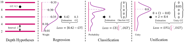
Figure 1: Comparison with different representations at a certain pixel. The purple curve represents different weights, probabilities, and unity of each depth hypothesis obtained by regression, classification and unification respectively. While the regression representation requires the exact weight of each hypothesis to regress the depth, the classification representation only cares about which hypothesis has the maximum probability and unification only needs to know the proximity with the maximum unity. $CE$ denotes cross-entropy, and $UFL$ refers to Unified Focal Loss (Sec. 3.3).

In this paper, we seek to unify the advantages of regression and classification, that is, we hope that the model can accurately predict the depth while maintaining robustness. There is a fact that the depth hypothesis close to the ground-truth has more potential knowledge, while that of other remaining hypotheses is limited or even harmful due to the wrong induction of multimodal [42]. Motivated by this, we present that estimating the weights for all depth hypotheses is redundant, and the model only needs to do regression on the optimal depth hypothesis that the representative depth interval (referring to the upper area until the next larger depth hypothesis) contains the ground truth depth. To achieve this, we propose a unified representation for depth, termed Unification. As shown in Fig. 1, unlike regression, the loss is executed on the regularized probability volume directly, and different from classification, our method estimates the Unity (What we call), whose label is composed by at most one non-zero continuous target $(0\sim 1)$, to simultaneously represent the location of optimal depth hypothesis and its offset to the ground-truth depth. We take proximity (defined as the complement of the offset between ground-truth and optimal depth hypothesis) to characterize the non-zero target in unity label, which is more efficient than purely using offset. The detailed comparisons are in Supp. Mat.

Moreover, we note that this unified representation faces an undeniable sample imbalance in both category and hardness. While Focal Loss (FL) [19] is the common solution proposed in the detection field, which is tailored to the traditional discrete label, the more general form (GFL) is proposed in [17, 40] to deal with the continuous label. Even though GFL has demonstrated its performance, we hold the belief that it has an obvious limitation in distinguishing hard and easy samples due to ignoring the magnitude of ground-truth. To this end, we put forward a more reasonable and unified form, called Unified Focal Loss (UFL), after thorough analysis to better address these challenges. In this way, the traditional FL can be regarded as a special case of UFL, while GFL is its imperfect expression.

To demonstrate the superiority of our proposed modules, we present a coarse-to-fine framework termed UniMVSNet (or UnifiedMVSNet), named for its unification of depth representation and focal loss, which replaces the traditional representation of recent works [5, 34, 9] with Unification and adopts UFL for optimization. Extensive experiments show that our model surpasses all previous MVS methods and achieves state-of-the-art performance on both DTU [1] and Tanks and Temples [14] benchmarks.

2 Related Works

Traditional MVS methods. Taking the output scene representation as an axis of taxonomy, there are mainly four types of classic MVS methods: volumetric [27, 15], point cloud based [16, 7], mesh based [6] and depth map based [3, 25, 24, 31, 8]. Among them, the depth map based method is the most flexible one. Instead of operating in the 3D domain, it degenerates the complex problem of 3D geometry reconstruction to depth map estimation in the 2D domain. Moreover, as the intermediate representation, the estimated depth maps of all individual images can be merged into a consistent point cloud [22] or a volumetric reconstruction [23], and the mesh can even be further reconstructed.

Learning-based MVS methods. While the traditional MVS pipeline mainly relies on hand-crafted similarity metrics, recent works apply deep learning for superior performance on MVS. SurfaceNet [11] and LSM [12] are the first proposed volumetric learning-based MVS pipelines to regress surface voxels from 3D space. However, they are restricted to memory which is the common drawback of the volumetric representation. Most recently, MVSNet [35] first realizes an end-to-end memory low-sensitive pipeline based on 3D cost volumes. This pipeline mainly consists of four steps: image feature extraction by 2D CNN, variance-based cost aggregation by homography warping, cost regularization through 3D CNN, and depth regression. To further excavate the potential capacity of this pipeline, some variants of MVSNet have been proposed, e.g., [36, 9, 5, 34] are proposed to reduce the memory requirement through RNN or coarse-to-fine manner, [20, 38] are proposed to adaptively re-weight the contribution of different pixels in cost aggregation. Meanwhile, all existing methods are based on one of the two complementary of classification and regression to infer depth. In this paper, we propose a novel unified representation to integrate their advantages.

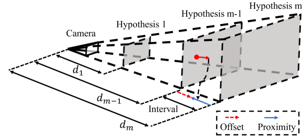
Figure 2: Illustration of our Unification. The $(m-1)_{th}$ hypothesis is the optimal hypothesis for red point.

3 Methodology

This section will present the main contributions of this paper in detail. We first review the common pipeline of the learning-based MVS approach in Sec. 3.1, then introduce the proposed unified depth representation in Sec. 3.2 and unified focal loss in Sec. 3.3, and finally describe the detailed network architecture of our UniMVSNet in Sec. 3.4.

3.1 Review of Learning-based MVS

Most end-to-end learning-based MVS methods are inherited from MVSNet [35], which constructs an elegant and effective pipeline to infer the depth $\mathbf{D}\in\mathbb{R}^{H^{\prime}\times W^{\prime}}$ of the reference image $\mathbf{I}_{1}$. Given multiple images $\{\mathbf{I}_{i}\in\mathbb{R}^{C\times H\times W}\}_{i=1}^{N}$ of a scene taken from $N$ different viewpoints, image features of all images $\{\mathbf{F}_{i}\in\mathbb{R}^{C^{\prime}\times H^{\prime}\times W^{\prime}}\}_{i=1}^{N}$ are first extracted through a 2D network with shared weights. As mentioned above, the learning-based method is based on the 3D cost volume, and the depth hypothesis of $M$ layers $\{\mathbf{d}_{i}\in\mathbb{R}^{H^{\prime}\times W^{\prime}}\}_{i=1}^{M}$ is sampled from the whole known depth range to achieve this, where $\mathbf{d}_{1}$ represents the minimum depth and $\mathbf{d}_{M}$ represents the maximum depth. With this hypothesis, feature volumes $\{\mathbf{V}_{i}\in\mathbb{R}^{M\times C^{\prime}\times H^{\prime}\times W^{\prime}}\}_{i=1}^{N}$ can be constructed in 3D space via differentiable homography by warping 2D image features of source images to the reference camera frustum. The homography between the feature maps of $i_{th}$ view and the reference feature maps at depth $d$ is expressed as:

$$\mathbf{H}_{i}(d)=d\mathbf{K}_{i}\mathbf{T}_{i}\mathbf{T}_{1}^{-1}\mathbf{K}_{1}^{-1}$$ (1)

where $\mathbf{K}$ and $\mathbf{T}$ refer to camera intrinsics and extrinsics respectively.

To handle arbitrary number of input views, the multiple feature volumes $\{V_{i}\}_{i=1}^{N}$ need to be aggregated to one cost volume $\mathbf{C}\in\mathbb{R}^{M\times C^{\prime}\times H^{\prime}\times W^{\prime}}$. The aggregation strategy consists two dominant groups: statistical and adaptive. The variance-based mapping is a typical statistical aggregation:

$$\mathbf{C}=\frac{1}{N}\sum_{i=1}^{N}(\mathbf{V}_{i}-\mathbf{\bar{V}})^{2}$$ (2)

Where $\mathbf{\bar{V}}$ denotes the average feature volume. Furthermore, the adaptive aggregation is proposed to re-weight the contribution of different pixels, which can be modeled as:

$$\mathbf{C}=\frac{1}{N-1}\sum_{i=2}^{N}\mathcal{W}_{i}\odot(\mathbf{V}_{i}-\mathbf{V}_{1})^{2}$$ (3)

where $\mathcal{W}$ is the learnable weight generated by an auxiliary network, and $\odot$ denotes element-wise multiplication.

The matching cost between the reference view and all source views under each depth hypothesis has been encoded into the cost volume, which is required to be further refineed to generate a probability volume $\mathbf{P}\in\mathbb{R}^{M\times H^{\prime}\times W^{\prime}}$ through a softmax-based regularization network. Concretely, the probability volume is treated as the weight of depth hypotheses in regression methods and the depth at pixel $(x,y)$ is calculated as the sum of the weighted hypotheses as:

$$\mathbf{D}^{x,y}=\sum_{d=\mathbf{d}_{1}^{x,y}}^{\mathbf{d}_{M}^{x,y}}d\mathbf{P}(d)^{x,y}$$ (4)

and the model is constrained by the L1 loss between $\mathbf{D}$ and the ground-truth depth. In classification methods, $\mathbf{P}$ refers to the probability of depth hypotheses and the depth is estimated as the hypothesis whose probability is maximum:

$$\mathbf{D}^{x,y}=\mathop{\arg\max}_{d\in\{\mathbf{d}_{i}^{x,y}\}_{i=1}^{M}}\mathbf{P}(d)^{x,y}$$ (5)

and the model is trained by the cross-entropy loss between $\mathbf{P}$ and the ground-truth one-hot probability volume.

In traditional one-stage methods, compared with original input images, the depth map is either downsized during feature extraction [35] or before the input [38] to save memory, while in the coarse-to-fine method [9, 34, 5], it’s a multi-scale result $\{\mathbf{D}_{i}\}_{i=1}^{L}$ with incremental resolution generated by repeating the above pipeline $L$ times. The multi-scale is realized by a FPN-like [18] feature extraction network, and the depth hypothesis with decreasing depth range is sampled based on the depth map generated in the previous stage.

Input: Ground-truth depth $\mathbf{D}_{gt}\in\mathbb{R}^{H^{\prime}\times W^{\prime}}$; Depth hypotheses $\{\mathbf{d}_{i}\in\mathbb{R}^{H^{\prime}\times W^{\prime}}\}_{i=1}^{M}$.

Output: Ground-truth Unity $\{\mathbf{U}_{i}\in\mathbb{R}^{H^{\prime}\times W^{\prime}}\}_{i=1}^{M}$.

Initialization : Depth interval $r=0$.

1 for $i=1$ to $M$ do

2       for $(x,y)=(1,1)$ to $(H^{\prime},W^{\prime})$ do

3             if $i<M$ then

4                   $r=\mathbf{d}_{i+1}^{x,y}-\mathbf{d}_{i}^{x,y}$ ;

5                  

6             end if

7            if $\mathbf{d}_{i}^{x,y}\leq\mathbf{D}_{gt}^{x,y}$ and $\mathbf{d}_{i}^{x,y}+r>\mathbf{D}_{gt}^{x,y}$ then

8                   $\mathbf{U}_{i}^{x,y}=1-\frac{\mathbf{D}_{gt}^{x,y}-\mathbf{d}_{i}^{x,y}}{r}$ ;

9                  

10            else

11                   $\mathbf{U}_{i}^{x,y}=0$ ;

12                  

13             end if

14            

15       end for

16      

17 end for

return $\{\mathbf{U}_{i}\}_{i=1}^{M}$.

Algorithm 1 Unity Generation

Input: Estimated unity $\{\mathbf{\widehat{U}}_{i}\in\mathbb{R}^{H^{\prime}\times W^{\prime}}\}_{i=1}^{M}$; Depth hypotheses $\{\mathbf{d}_{i}\in\mathbb{R}^{H^{\prime}\times W^{\prime}}\}_{i=1}^{M}$.

Output: Regressed Depth $\mathbf{D}\in\mathbb{R}^{H^{\prime}\times W^{\prime}}$.

Initialization : Depth interval $r=0$.

1 for $(x,y)=(1,1)$ to $(H^{\prime},W^{\prime})$ do

2       Optimal hypothesis index $o=\mathop{\arg\max}\limits_{i\in\{1,\cdots,M\}}\mathbf{\widehat{U}}_{i}^{x,y}$;

3       Optimal hypothesis $d=\mathbf{d}_{o}^{x,y}$ ;

4       if $o<M$ then

5             $r=\mathbf{d}_{o+1}^{x,y}-\mathbf{d}_{o}^{x,y}$ ;

6            

7      else

8             // previous interval for the last hypothesis  

9            $r=\mathbf{d}_{o}^{x,y}-\mathbf{d}_{o-1}^{x,y}$ ;

10            

11       end if

12      Offset $off=(1-\mathbf{\widehat{U}}_{o}^{x,y})\times r$ ;

13       Depth $\mathbf{D}^{x,y}=d+off$ ;

14      

15 end for

return $\mathbf{D}$.

Algorithm 2 Unity Regression

Figure 3: Hardness measurement of different samples. Four typical samples with different ground-truth $q$ and different estimation $u$.

3.2 Unified Depth Representation

As aforementioned, the regression method tends to overfit due to its indirect learning cost volume and ambiguity in the correspondence between depth and the weight combination. For the classification method, although it can constrain the cost volume directly, it cannot predict exact depth like regression methods due to its discrete prediction. In this paper, we found that they can complement each other, and we unify them successfully through our unified depth representation, as shown in Fig. 2. We recast the depth estimation as a multi-label classification task, in which the model needs to classify which hypothesis is the optimal one and regress the proximity for it. In other words, we first adopt classification to narrow the depth range of the final regression, but they are executed simultaneously in our implementation. Therefore, the model in our Unification representation is able to estimate an accurate depth like regression methods, and it also directly optimizes the cost volume like classification methods. Below, we will introduce how to generate the ground-truth unity from ground-truth depth (Unity generalization), and how to regress the depth from the estimated unity (Unity regression).

Unity generation: As shown in Fig. 1, ground-truth unity $\{\mathbf{U}_{i}\}_{i=1}^{M}$ is a more general form of one-hot label peaked at the optimal depth hypothesis whose depth interval contains ground-truth depth. The at most one non-zero target is a continuous number and represents the proximity of the optimal hypothesis to ground-truth depth. The detail of unity generation is shown in Algorithm 1, which is one more step of proximity calculation than the one-hot label generation in classification methods.

Unity regression: Unlike the traditional way of predicting the probability volume by softmax operators, unification representation estimated it through sigmoid operators. Here, we disassemble the estimated probability volume $\mathbf{P}$ into the estimated unity $\{\mathbf{\widehat{U}}_{i}\}_{i=1}^{M}$ along the $M$ dimension. To regress the depth, we first select the optimal hypothesis with the maximum unity at each pixel, then calculate the offset to ground-truth depth, and finally fuse the estimated depth. The detailed procedure is shown in Algorithm 2.

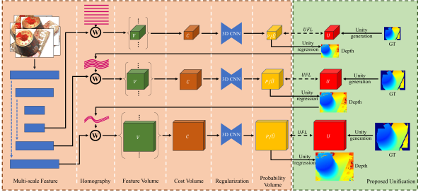
Figure 4: Illustration of UniMVSNet. This is a typical coarse-to-fine framework. The part with pink background is inherited from existing methods, and the green part is our novel modules. The depth hypothesis is represented by the red curve for convenience.

3.3 Unified Focal Loss

Generally, the depth hypothesis of MVS models will be sampled quite densely to ensure the accuracy of the estimated depth, which will cause obvious sample imbalance due to only one positive sample (the at most one non-zero target) among hundreds of hypotheses. Meanwhile, the model needs to pay more attention to hard samples to prevent overfitting. Relevant Focal Loss (FL) [19] has been proposed to solve these two problems, which automatically distinguishes hard samples through the estimated unity $u\in[0,1]$ and rebalances the sample through tunable parameter $\alpha$ and $\gamma$. Here, we discuss a certain pixel for convenience. The typical definition of FL is:

$${\rm FL}(u,q)=\begin{cases}-\alpha(1-u)^{\gamma}\log(u),&q=1\\ -(1-\alpha)u^{\gamma}\log(1-u),&\text{else}\end{cases}$$ (6)

where $q\in\{0,1\}$ is the discrete target. Therefore, the traditional FL is not suitable for our continuous situation. To enable successful training under the case of our representation, we borrow the main idea from FL. Above all, the binary cross-entropy $-\log(u)$ or $-\log(1-u)$ needs to be extended to its complete form ${\rm BCE}(u,q)=-q\log(u)-(1-q)\log(1-u)$. Correspondingly, the scaling factor should also be adjusted appropriately. The generalized FL form (GFL) obtained through these two steps is:

$${\rm GFL}(u,q)=\begin{cases}\alpha|q-u|^{\gamma}{\rm BCE}(u,q),&q>0\\ (1-\alpha)u^{\gamma}{\rm BCE}(u,q),&\text{else}\end{cases}$$ (7)

where $q\in[0,1]$ is the continuous target. This advanced version is currently adopted by some existing methods with different names, e.g., QFL in [17] or VFL in [40]. But in this paper, we point out that this implementation is not perfect in scaling hard and easy samples, because they ignore the magnitude of the ground-truth.

As shown in Fig. 3, the first two samples will be considered the hardest under the absolute error $|q-u|$ measurement in GFL. However, the absolute error cannot distinguish samples with different targets. Even if the first two samples in Fig. 3 have the same absolute error, this error obviously has a smaller effect on the first sample due to its larger ground-truth. To solve this ambiguity, we further improve the scaling factor in GFL through relative error and propose our naive version of Unified Focal Loss (UFL) just as:

$${\rm UFL}(u,q)=\begin{cases}\alpha(\frac{|q-u|}{q^{+}})^{\gamma}{\rm BCE}(u,q),\!&q>0\\ (1-\alpha)(\frac{u}{q^{+}})^{\gamma}{\rm BCE}(u,q),\!&\text{else}\end{cases}$$ (8)

where $q^{+}\in(0,1]$ is the positive target. It can be seen from Eq. 8 that FL is a special case of UFL when the positive target is the constant 1.

Moreover, we noticed that the range of scaling factor $\frac{|q-u|}{q^{+}}$ is $[0,+\infty)$, which may lead to a special case like the last sample in Fig. 3. Even a small number of such samples will overwhelm the loss and computed gradients due to their huge scaling factor. In this paper, we solve this problem by introducing a dedicated function to control the range of the scaling factor. Meanwhile, to keep the precious positive learning signals, we adopt an asymmetrical scaling strategy. And the complete UFL can be modeled as:

$${\rm UFL}(u,q)\!=\!\begin{cases}\alpha^{+}(S_{b}^{+}(\frac{|q-u|}{q^{+}}))^{\gamma}{\rm BCE}(u,q),\!&q>0\\ \alpha^{-}(S_{b}^{-}(\frac{u}{q^{+}}))^{\gamma}{\rm BCE}(u,q),\!&\text{else}\end{cases}$$ (9)

where the dedicated function $S_{b}(x)$ is designed as the sigmoid-like function ($1/(1+b^{-x})$) with a base of $b$ in this paper.

3.4 UniMVSNet

It’s straightforward to apply our Unification and UFL to existing learning-based MVS methods. To illustrate the effectiveness and flexibility of the proposed modules, we build the UniMVSNet, whose framework is depicted in Fig. 4, based on the coarse-to-fine strategy. This pipeline abides by the procedure reviewed in Sec. 3.1, except the depth representation and optimization.

Inherited from CasMVSNet [9], We adopt a FPN-like network to extract multi-scale features, and uniformly sample the depth hypothesis with a decreasing interval and a decreasing number. To better handle the unreliable matching in non-Lambertian regions, we adopt an adaptive aggregation method with negligible parameters increasing like [38] to aggregate the feature volumes warped by the differentiable homography. Meanwhile, we also apply multi-scale 3D CNNs to regularize the cost volume, and the generated probability volume $\mathbf{P}$ at each stage is treated as the estimated Unity $\{\mathbf{\widehat{U}}_{i}\}_{i=1}^{M}$ here, which can be further regressed to accurate depth as shown in Algorithm 2. It can be seen from Fig. 4 that UniMVSNet directly optimizes cost volume through UFL, which can effectively avoid the overfitting of indirect learning strategy in regression methods.

Training Loss. As shown in Fig. 4, we apply UFL to all stages and fuse them with different weights. The total loss can be defined as:

$$Loss=\sum_{i=1}^{L}\lambda_{i}\overline{{\rm UFL}}_{i}$$ (10)

where $\overline{{\rm UFL}}_{i}$ is the average of UFL of all valid pixels at stage $i$ and $\lambda_{i}$ denotes the weight of $\overline{{\rm UFL}}$ at $i_{th}$ stage.

4 Experiments

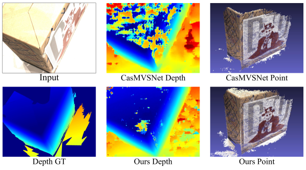
Figure 5: Depth estimation and point reconstruction of scan 13 on DTU. Our model produces more accurate and complete results.

Method	ACC.(mm)	Comp.(mm)	Overall(mm)
Furu [7]	0.613	0.941	0.777
Gipuma [8]	0.283	0.873	0.578
COLMAP [24, 25]	0.400	0.664	0.532
SurfaceNet [11]	0.450	1.040	0.745
MVSNet [35]	0.396	0.527	0.462
P-MVSNet [20]	0.406	0.434	0.420
R-MVSNet [36]	0.383	0.452	0.417
Point-MVSNet [4]	0.342	0.411	0.376
AA-RMVSNet [30]	0.376	0.339	0.357
CasMVSNet [9]	0.325	0.385	0.355
CVP-MVSNet [34]	0.296	0.406	0.351
UCS-Net [5]	0.338	0.349	0.344
UniMVSNet (ours)	0.352	0.278	0.315

Table 1: Quantitative results on DTU evaluation set. Best results in each category are in bold. Our model ranks first in terms of Completeness and Overall metrics.

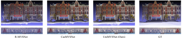
Figure 6: Qualitative results of scan 15 on DTU. The top row shows the point clouds generated by different methods and the ground-truth, and the bottom row shows a more detailed local region corresponding to the red rectangle.

Method	Intermediate									Advanced
	Mean	Fam.	Fra.	Hor.	Lig.	M60	Pan.	Pla.	Tra.	Mean	Aud.	Bal.	Cou.	Mus.	Pal.	Tem.
Point-MVSNet [4]	48.27	61.79	41.15	34.20	50.79	51.97	50.85	52.38	43.06	-	-	-	-	-	-	-
PatchmatchNet [29]	53.15	66.99	52.64	43.24	54.87	52.87	49.54	54.21	50.81	32.31	23.69	37.73	30.04	41.80	28.31	32.29
UCS-Net [5]	54.83	76.09	53.16	43.03	54.00	55.60	51.49	57.38	47.89	-	-	-	-	-	-	-
CVP-MVSNet [34]	54.03	76.50	47.74	36.34	55.12	57.28	54.28	57.43	47.54	-	-	-	-	-	-	-
P-MVSNet [20]	55.62	70.04	44.64	40.22	65.20	55.08	55.17	60.37	54.29	-	-	-	-	-	-	-
CasMVSNet [9]	56.84	76.37	58.45	46.26	55.81	56.11	54.06	58.18	49.51	31.12	19.81	38.46	29.10	43.87	27.36	28.11
ACMP [32]	58.41	70.30	54.06	54.11	61.65	54.16	57.60	58.12	57.25	37.44	30.12	34.68	44.58	50.64	27.20	37.43
$D^{2}$HC-RMVSNet [33]	59.20	74.69	56.04	49.42	60.08	59.81	59.61	60.04	53.92	-	-	-	-	-	-	-
VisMVSNet [41]	60.03	77.40	60.23	47.07	63.44	62.21	57.28	60.54	52.07	33.78	20.79	38.77	32.45	44.20	28.73	37.70
AA-RMVSNet [30]	61.51	77.77	59.53	51.53	64.02	64.05	59.47	60.85	55.50	33.53	20.96	40.15	32.05	46.01	29.28	32.71
EPP-MVSNet [21]	61.68	77.86	60.54	52.96	62.33	61.69	60.34	62.44	55.30	35.72	21.28	39.74	35.34	49.21	30.00	38.75
UniMVSNet (ours)	64.36	81.20	66.43	53.11	63.46	66.09	64.84	62.23	57.53	38.96	28.33	44.36	39.74	52.89	33.80	34.63

Table 2: Quantitative results of F-score on Tanks and Temples benchmark. Best results in each category are in bold. “Mean” refers to the mean F-score of all scenes (higher is better). Our model outperforms all previous MVS methods with a significant margin on both Intermediate and Advanced set.

This section demonstrates the start-of-the-art performance of UniMVSNet with comprehensive experiments and verifies the effectiveness of the proposed Unification and UFL through ablation studies. We first introduce the datasets and implementation and then analyze our results.

Datasets. We evaluate our model on DTU [1] and Tanks and Temples [14] benchmark and finetune on BlendedMVS [37]. (a) DTU is an indoor MVS dataset with 124 different scenes scanned from 49 or 64 views under 7 different lighting conditions with fixed camera trajectories. We adopt the same training, validation, and evaluation split as defined in [35]. (b) Tanks and Temples is collected in a more complex realistic environment, and it’s divided into the intermediate and advanced set. While intermediate set contains 8 scenes with large-scale variations, advanced set has 6 scenes. (c) BlendedMVS is a large-scale synthetic dataset, which is consisted of 113 indoor and outdoor scenes and is split into 106 training scenes and 7 validation scenes.

Implementation. Following the common practice, we first train our model on the DTU training set and evaluate on DTU evaluation set, and then finetune our model on BlendedMVS before validating the generalization of our approach on Tanks and Temples. The input view selection and data pre-processing strategies are the same as [35]. Meanwhile, we utilize the finer DTU ground-truth as [30]. In this paper, UniMVSNet is implemented in 3 stages with 1/4, 1/2 ,and 1 of original input image resolution respectively. We follow the same configuration (e.g., depth interval) of the model at each stage as [9] in both training and evaluation of DTU. When training on DTU, the number of input images is set to $N=5$ and the image resolution is resized to $640\times 512$. To emphasize the contribution of positive signals, we set $\alpha^{+}=1$, and scale the range of $S_{5}^{+}$ to $[1,3)$ and $S_{5}^{-}$ to $[0,1)$. The other tunable parameters in UFL are configured stage-wise, e.g., $\alpha^{-}$ is set to 0.75, 0.5, and 0.25, and $\gamma$ is set to 2, 1, and 0 from the coarsest stage to the finest stage.. We optimize our model for 16 epochs with Adam optimizer [13], and the initial learning rate is set to 0.001 and decayed by 2 after 10, 12, and 14 epochs. During the evaluation of DTU, we also resize the input image size to $1152\times 864$ and set the number of the input images to 5. We report the standard metrics (accuracy, completeness, and overall) proposed by the official evaluation protocol [1]. Before testing on Tanks and Temples benchmark, we finetune our model on BlendedMVS for 10 epochs. We take 7 images as the input with the original size of $768\times 576$. For benchmarking on Tanks and Temples, the number of depth hypotheses in the coarsest stage is changed from 48 to 64, and the corresponding depth interval is set to 3 times as the interval of [35]. We set the number of input images to 11 and report the F-score metric

4.1 Results on DTU

Similar to previous methods [35, 36, 9], we introduce photometric and geometric constraints for depth map filtering. The probability threshold and the number of consistent views are set to 0.3 and 3 respectively, which is the same as [36]. The final 3D point cloud is obtained through the same depth map fusion method as [35, 36, 9].

We compare our method to those traditional and recent learning-based MVS methods. The quantitative results on the DTU evaluation set are summarized in Tab. 1, which indicates that our method has made great progress in performance. While Gipuma [8] ranks first in the accuracy metric, our method outperforms all methods on the other two metrics significantly. Depth map estimation and point reconstruction of a reflective and low-textured sample are shown in Fig. 5, which shows that our model is more robust on the challenge regions. Figure 6 shows some qualitative results compared with other methods. We can see that our model can generate more complete point clouds with finer details.

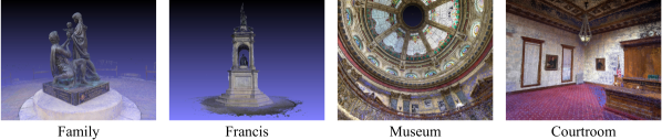
Figure 7: Qualitative results of some scenes on Tanks and Temples.

Method

Representation

Loss Function

Aggregation

FGT

Input

ACC.(mm)

Comp.(mm)

Overall.(mm)

Reg

Cla

Uni

L1

CE

BCE

GFL

UFL

Adaptive

Variance

Baseline (Reg)

✓

✓

✓

3

0.369

0.317

0.343

Baseline (Reg)

✓

✓

✓

5

0.368

0.312

0.340

Baseline (Cla)

✓

✓

✓

5

0.425

0.285

0.355

Baseline (Uni)

✓

✓

✓

5

0.372

0.282

0.327

Baseline (Uni) + GFL

✓

✓

✓

5

0.361

0.289

0.325

Baseline (Uni) + UFL

✓

✓

✓

5

0.353

0.287

0.320

Baseline (Uni) + UFL + AA

✓

✓

✓

5

0.355

0.279

0.317

Baseline (Uni) + UFL + AA + FGT

✓

✓

✓

✓

5

0.352

0.278

0.315

Table 3: Ablation results on DTU evaluation set. “AA” and “FGT” refer to adaptive aggregation and finer ground-truth respectively. “Baseline (Reg)” is the original CasMVSNet [9]. We set the confidence threshold and the consistent views to 0.3 and 3 for all models.

4.2 Results on Tanks and Temples

As the common practice, we verify the generalization ability of our method on Tanks and Temples benchmark using the model finetuned on BlendedMVS. We adopt a depth map filtering strategy similar to that of DTU, except for the geometric constraint. Here, we follow the dynamic geometric consistency checking strategies proposed in [33]. Through this dynamic method, those pixels with fewer consistent views but smaller reprojection errors and those with larger errors but more consistent views will also survive.

The corresponding quantitative results on both intermediate and advanced sets are reported in Tab. 2. Our method achieves state-of-the-art performance among all existing MVS methods and yields first place in most scenes. Notably, our model outperforms the previous best model by 2.68 points and 3.24 points on the intermediate and advanced sets. Such obvious advantages just show that our model not only has the best performance but also exhibits the strongest generalization and robustness. The qualitative point cloud results are visualized in Fig. 7.

4.3 Ablation Studies

As aforementioned, we adopt some extra strategies (e.g., adaptive aggregation and finer ground-truth) that have been adopted by recent methods [30, 38] to train our model for a fair comparison with them. However, this may not be fair to those methods inherited only from MVSNet. In this section, we will prove through extensive ablation studies that even if these strategies are eliminated, our method still has a significant improvement. We use our baseline CasMVSNet [9], whose original representation is regression, as the backbone and changing various components, e.g., depth representation, optimization, aggregation, and ground-truth. And we adopt 5 input views for all models for a fair comparison.

Benefits of Unification. As shown in Tab. 3, significant progress can be made even if purely replacing the traditional depth representation with our unification. Meanwhile, unification is more robust when the hypothesis range of the finer stage doesn’t cover the ground-truth depth. In this case, the target unity of the unification representation generated by Algorithm 1 is all zero, which is a correct supervision signal anyway, and the traditional representation will generate an incorrect supervision signal to pollute the model training. Meanwhile, our Unification can also generate sharp depth on object boundaries like [28].

Benefits of UFL. Applying Focal Loss to our representation can effectively overcome the sample imbalance problem. It can be seen from Tab. 3 that GFL has a huge benefit to accuracy, albeit with a slight loss of completeness. And our UFL can further improve the accuracy and completeness significantly on the basis of GFL. More ablation results about UFL are shown in Supp. Mat.

Other strategies and less data. Tab. 4 shows that our Unification performs better and is more concise compared to other strategies. Meanwhile, we still achieve excellent performance even with only 50% of the training data.

Method	Confidence	Consistent View	ACC.(mm)	Comp.(mm)	Overall(mm)
Baseline (Cla) + Regress finetune	0.3	3	0.371	0.295	0.333
Baseline (Uni) + UFL (50% data)	0.3	3	0.364	0.284	0.324

Table 4: Some other Ablation results.

5 Conclusion

In this paper, we propose a unified depth representation and a unified focal loss to promote the effectiveness of multi-view stereo. Our Unification can recover finer 3D scene benefits from the direct learning cost volume, and UFL is able to capture more fine-grained indicators for rebalancing samples and deal with continuous labels more reasonably. What’s more valuable is that these two modules don’t impose any memory or computational costs. Each plug-and-play module can be easily integrated into the existing MVS framework and achieve significant performance improvements, and we have shown this through our UniMVSNet. In the future, we plan to explore the integration of our modules into stereo matching or monocular field and look for more concise loss functions.
Acknowledgements. Thanks to the National Natural Science Foundation of China 62072013 and U21B2012, Shenzhen Research Projects of JCYJ20180503182128089 and 201806080921419290, Shenzhen Cultivation of Excellent Scientific and Technological Innovation Talents RCJC20200714114435057,Shenzhen Fundamental Research Program (GXWD20201231165807007-20200806163656003). In addition, we thank the anonymous reviewers for their valuable comments.

Supplementary Material

A More Explanation of Unified Focal Loss

As shown in Equation (9), the dedicated function to control the range of scaling factor is designed as the sigmoid-like function as:

$$S_{b}(x)=\frac{1}{(1+b^{-x})}$$ (a)

where $x=\frac{|q-u|}{q^{+}}$ in this paper and its range is $[0,+\infty)$, therefore, the range of $S_{b}(x)$ is $[0.5,1)$. As aforementioned, we adopt an asymmetrical scaling strategy to protect the precious positive learning signals and scale the range of $S_{5}^{+}$ to $[1,3)$ and $S_{5}^{-}$ to $[0,1)$. The detailed implementation of $S_{5}^{+}$ is:

$$S_{5}^{+}(x)=4\times(\frac{1}{1+5^{-x}}-0.5)+1$$ (b)

and the detailed implementation of $S_{5}^{-}$ is:

$$S_{5}^{-}(x)=2\times(\frac{1}{1+5^{-x}}-0.5)$$ (c)

B Finer DTU Ground-truth

As mentioned in our main paper, we adopt the finer ground-truth to train our model additionally for a fair comparison with the start-of-the-art methods [30]. The refinement of each DTU ground-truth is achieved by cross-filtering with its neighbor viewpoints. For convenience, we directly adopt the processed results provided in [30], and we only adopt the mask which indicates the validity of each point. Concretely, we adopt the union of the mask provided in [9, 35] and the up-sampled mask provided in [30] as the final mask.

C More Ablation Studies on DTU Dataset

Here, we perform more ablation studies on DTU to show you more information about our implementation.

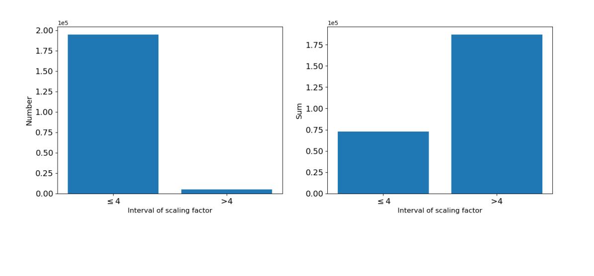
Figure A: The statistics of scaling factor $x=\frac{|q-u|}{q^{+}}$ in Eq. 8.

The scaling factor in UFL. The range of scaling factor in Eq. 8 is $[0,+\infty)$. We count the average number and sum of scaling factors that fall in different intervals. As shown in Fig. A, most of the scaling factors are less than 4 (Left figure). Even though, those small fractions of larger scaling factors take more weight (Right figure). This results in those abnormally large scaling factors occupying the model’s training, and lead to difficulty in model convergence and extremely poor performance. Therefore, we introduce a dedicated function to control the scaling factors’ range.

The dedicated function in UFL. As described in our main paper, we design the positive dedicated function as Eq. b and negative dedicated function as Eq. c. In fact, this final implementation is confirmed under our more experimental results. As shown in Tab. A, compared to adopting a common sigmoid function with a base $e$, it’s better to use a dedicated function with a base 5. Meanwhile, scaling the range of dedicated function to $[1,3)$ is better than $[1,2)$. As shown in Fig. B, the base number controls the speed at which the function converges to the maximum value. The smaller the base number, the slower the convergence. In our experiments, we found that most of the points whose $x=\frac{|q-u|}{q^{+}}$ is in the interval $[0,4]$, so the scaling value calculated by the dedicated function needs to be distinguishable for the points in this interval, and we set $b=5$ in this paper. To be honest, we have only conducted a limited number of the base number the range of dedicated function as shown in Tab. A due to the time and resource considerations, and we believe there will be more powerful configurations.

Base Number	Range	ACC.(mm)	Comp.(mm)	Overall(mm)
$e$	$[1,2)$	0.354	0.282	0.318
5	$[1,2)$	0.354	0.280	0.317
5	$[1,3)$	0.352	0.278	0.315

Table A: Ablation results of dedicated function. While the base number is ablated for both the positive and negative dedicated function, we only ablate the range of positive dedicated function.

The tunable parameter in UFL. Tunable parameters in UFL like $\alpha$ and $\lambda$ are also important for rebalancing samples. As mentioned in our main paper, we always set $\alpha^{+}=1$ to protect the positive learning signals and configure other tunable parameters stage by stage due to the different number of depth hypotheses. In our implementation, we set the number of depth hypotheses to 48, 32, and 8 from stage1 to stage3. Apparently, the sample imbalance in stage1 is the most challenging, while it’s the most relaxing or even negligible in stage3. As shown in Tab. B, applying the same configuration across all stages performs the worst which indicates that the imbalances faced by different stages are different.

Proximity $\mathcal{VS}$. Offset. Different from the Regression and Classification, we propose Unification to classify the optimal depth hypothesis and regress its offset to ground-truth depth simultaneously. As shown in Fig. C, there are two ways to regress the offset. The first is to predict proximity which is the complement of the offset and is also the method we adopt in this paper. The second is to directly estimate the offset. The comparison results between them are shown in Tab. C. We can see that adopting proximity to regress the offset indirectly is much more powerful than purely using offset. As mentioned in our main paper, our Unification can be decomposed into two parts: classify the optimal depth hypothesis first and then regress the proximity for it. We infer that the reason why proximity is better than offset is the positive relationship between the magnitude of proximity and the quality of the classified optimal depth hypothesis in the first step. Meanwhile, we think that there should be better settings to improve the performance of using offset, but we have not made more attempts here.

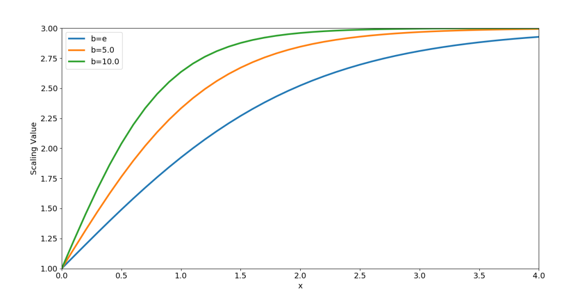
Figure B: The scaling value obtained through the positive dedicated function under different base numbers.

$\alpha^{-}$			$\lambda$			ACC.(mm)	Comp.(mm)	Overall(mm)
stage1	stage2	stage3	stage1	stage2	stage3
0.75	0.75	0.75	2	2	2	0.347	0.325	0.336
1	1	1	2	1	0	0.366	0.282	0.324
0.75	0.50	0.25	2	1	0	0.353	0.287	0.320

Table B: Ablation results of tunable parameters. These experiments are conducted on the model with only our Unification and UFL, and don’t adopt the finer DTU ground-truth or adaptive aggregation.

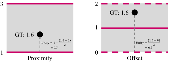
Figure C: Two available solutions to generate Unity (supervised signal) from the ground-truth depth. For proximity, we use the interval above the depth hypothesis as its regression interval, and for offset, use the area where the depth hypothesis is the median value as the regression interval.

Method	ACC.(mm)	Comp.(mm)	Overall(mm)
Offset	0.429	0.336	0.383
Proximity	0.372	0.282	0.327

Table C: Comparison of proximity and offset. These experiments are conducted on the model only using our Unification.

D More Comparisons between Unification, Classification and Regression

(1) Regression methods are harder to converge and have a greater risk of overfitting due to its indirect learning strategy, which has been studied in [42]. Meanwhile, they tend to generate smooth depth in object boundaries, because they treat the depth as the expectation of the depth hypotheses. However, they can achieve sub-pixel depth estimation, therefore, they have better accuracy. (2) Classification methods cannot generate accurate depth due to their discrete prediction, but they constrain the cost volume directly and achieve better completeness. (3) Our unification is exactly the complement of these two approaches. Take the essence, get rid of the dross. On the one hand, We directly constrain the cost volume to keep the model robust and pick the regression interval with the maximum unity to maintain the sharpness of the object boundary. On the other hand, we regress the proximity in the picked regression interval to generate accurate depth. Therefore, our unification is hoped to achieve regression’s accuracy and classification’s completeness. The results shown in Tab. 3 just prove this.

E More Results on DTU Dataset

Figure D shows our additional point clouds reconstruction results. It can be seen that the point cloud reconstructed by our method has excellent accuracy and completeness.

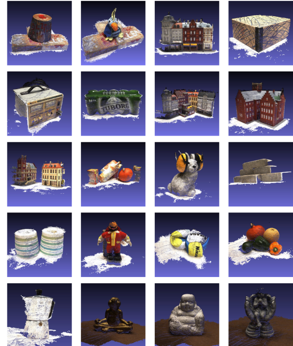
Figure D: More qualitative results on DTU dataset.

References

- [1] Henrik Aanæs, Rasmus Ramsbøl Jensen, George Vogiatzis, Engin Tola, and Anders Bjorholm Dahl. Large-scale data for multiple-view stereopsis. IJCV, 120(2):153–168, 2016.
- [2] Connelly Barnes, Eli Shechtman, Adam Finkelstein, and Dan B Goldman. Patchmatch: A randomized correspondence algorithm for structural image editing. ACM TOG, 28(3):24, 2009.
- [3] Neill DF Campbell, George Vogiatzis, Carlos Hernández, and Roberto Cipolla. Using multiple hypotheses to improve depth-maps for multi-view stereo. In ECCV, pages 766–779. Springer, 2008.
- [4] Rui Chen, Songfang Han, Jing Xu, and Hao Su. Point-based multi-view stereo network. In ICCV, pages 1538–1547, 2019.
- [5] Shuo Cheng, Zexiang Xu, Shilin Zhu, Zhuwen Li, Li Erran Li, Ravi Ramamoorthi, and Hao Su. Deep stereo using adaptive thin volume representation with uncertainty awareness. In CVPR, pages 2524–2534, 2020.
- [6] Pascal Fua and Yvan G Leclerc. Object-centered surface reconstruction: Combining multi-image stereo and shading. IJCV, 16(1):35–56, 1995.
- [7] Yasutaka Furukawa and Jean Ponce. Accurate, dense, and robust multiview stereopsis. IEEE TPAMI, 32(8):1362–1376, 2009.
- [8] Silvano Galliani, Katrin Lasinger, and Konrad Schindler. Massively parallel multiview stereopsis by surface normal diffusion. In ICCV, pages 873–881, 2015.
- [9] Xiaodong Gu, Zhiwen Fan, Siyu Zhu, Zuozhuo Dai, Feitong Tan, and Ping Tan. Cascade cost volume for high-resolution multi-view stereo and stereo matching. In CVPR, pages 2495–2504, 2020.
- [10] Po-Han Huang, Kevin Matzen, Johannes Kopf, Narendra Ahuja, and Jia-Bin Huang. Deepmvs: Learning multi-view stereopsis. In CVPR, pages 2821–2830, 2018.
- [11] Mengqi Ji, Juergen Gall, Haitian Zheng, Yebin Liu, and Lu Fang. Surfacenet: An end-to-end 3d neural network for multiview stereopsis. In ICCV, pages 2307–2315, 2017.
- [12] Abhishek Kar, Christian Häne, and Jitendra Malik. Learning a multi-view stereo machine. In NeurIPS, pages 365–376, 2017.
- [13] Diederik P Kingma and Jimmy Ba. Adam: A method for stochastic optimization. In ICLR, 2015.
- [14] Arno Knapitsch, Jaesik Park, Qian-Yi Zhou, and Vladlen Koltun. Tanks and temples: Benchmarking large-scale scene reconstruction. ACM TOG, 36(4):1–13, 2017.
- [15] Kiriakos N Kutulakos and Steven M Seitz. A theory of shape by space carving. IJCV, 38(3):199–218, 2000.
- [16] Maxime Lhuillier and Long Quan. A quasi-dense approach to surface reconstruction from uncalibrated images. IEEE TPAMI, 27(3):418–433, 2005.
- [17] Xiang Li, Wenhai Wang, Lijun Wu, Shuo Chen, Xiaolin Hu, Jun Li, Jinhui Tang, and Jian Yang. Generalized focal loss: Learning qualified and distributed bounding boxes for dense object detection. In NeurIPS, 2020.
- [18] Tsung-Yi Lin, Piotr Dollár, Ross Girshick, Kaiming He, Bharath Hariharan, and Serge Belongie. Feature pyramid networks for object detection. In CVPR, pages 2117–2125, 2017.
- [19] Tsung-Yi Lin, Priya Goyal, Ross Girshick, Kaiming He, and Piotr Dollár. Focal loss for dense object detection. In ICCV, pages 2980–2988, 2017.
- [20] Keyang Luo, Tao Guan, Lili Ju, Haipeng Huang, and Yawei Luo. P-mvsnet: Learning patch-wise matching confidence aggregation for multi-view stereo. In ICCV, pages 10452–10461, 2019.
- [21] Xinjun Ma, Yue Gong, Qirui Wang, Jingwei Huang, Lei Chen, and Fan Yu. Epp-mvsnet: Epipolar-assembling based depth prediction for multi-view stereo. In ICCV, pages 5732–5740, 2021.
- [22] Paul Merrell, Amir Akbarzadeh, Liang Wang, Philippos Mordohai, Jan-Michael Frahm, Ruigang Yang, David Nistér, and Marc Pollefeys. Real-time visibility-based fusion of depth maps. In ICCV, pages 1–8, 2007.
- [23] Richard A Newcombe, Shahram Izadi, Otmar Hilliges, David Molyneaux, David Kim, Andrew J Davison, Pushmeet Kohi, Jamie Shotton, Steve Hodges, and Andrew Fitzgibbon. Kinectfusion: Real-time dense surface mapping and tracking. In IEEE international symposium on mixed and augmented reality, pages 127–136, 2011.
- [24] Johannes L Schonberger and Jan-Michael Frahm. Structure-from-motion revisited. In CVPR, pages 4104–4113, 2016.
- [25] Johannes L Schönberger, Enliang Zheng, Jan-Michael Frahm, and Marc Pollefeys. Pixelwise view selection for unstructured multi-view stereo. In ECCV, pages 501–518, 2016.
- [26] Steven M Seitz, Brian Curless, James Diebel, Daniel Scharstein, and Richard Szeliski. A comparison and evaluation of multi-view stereo reconstruction algorithms. In CVPR, pages 519–528, 2006.
- [27] Steven M Seitz and Charles R Dyer. Photorealistic scene reconstruction by voxel coloring. IJCV, 35(2):151–173, 1999.
- [28] Fabio Tosi, Yiyi Liao, Carolin Schmitt, and Andreas Geiger. Smd-nets: Stereo mixture density networks. In CVPR, pages 8942–8952, 2021.
- [29] Fangjinhua Wang, Silvano Galliani, Christoph Vogel, Pablo Speciale, and Marc Pollefeys. Patchmatchnet: Learned multi-view patchmatch stereo. In CVPR, pages 14194–14203, 2021.
- [30] Zizhuang Wei, Qingtian Zhu, Chen Min, Yisong Chen, and Guoping Wang. Aa-rmvsnet: Adaptive aggregation recurrent multi-view stereo network. In ICCV, 2021.
- [31] Qingshan Xu and Wenbing Tao. Multi-scale geometric consistency guided multi-view stereo. In CVPR, pages 5483–5492, 2019.
- [32] Qingshan Xu and Wenbing Tao. Planar prior assisted patchmatch multi-view stereo. In AAAI, volume 34, pages 12516–12523, 2020.
- [33] Jianfeng Yan, Zizhuang Wei, Hongwei Yi, Mingyu Ding, Runze Zhang, Yisong Chen, Guoping Wang, and Yu-Wing Tai. Dense hybrid recurrent multi-view stereo net with dynamic consistency checking. In ECCV, pages 674–689, 2020.
- [34] Jiayu Yang, Wei Mao, Jose M Alvarez, and Miaomiao Liu. Cost volume pyramid based depth inference for multi-view stereo. In CVPR, pages 4877–4886, 2020.
- [35] Yao Yao, Zixin Luo, Shiwei Li, Tian Fang, and Long Quan. Mvsnet: Depth inference for unstructured multi-view stereo. In ECCV, pages 767–783, 2018.
- [36] Yao Yao, Zixin Luo, Shiwei Li, Tianwei Shen, Tian Fang, and Long Quan. Recurrent mvsnet for high-resolution multi-view stereo depth inference. In CVPR, pages 5525–5534, 2019.
- [37] Yao Yao, Zixin Luo, Shiwei Li, Jingyang Zhang, Yufan Ren, Lei Zhou, Tian Fang, and Long Quan. Blendedmvs: A large-scale dataset for generalized multi-view stereo networks. In CVPR, pages 1790–1799, 2020.
- [38] Hongwei Yi, Zizhuang Wei, Mingyu Ding, Runze Zhang, Yisong Chen, Guoping Wang, and Yu-Wing Tai. Pyramid multi-view stereo net with self-adaptive view aggregation. In ECCV, pages 766–782, 2020.
- [39] Zehao Yu and Shenghua Gao. Fast-mvsnet: Sparse-to-dense multi-view stereo with learned propagation and gauss-newton refinement. In CVPR, pages 1949–1958, 2020.
- [40] Haoyang Zhang, Ying Wang, Feras Dayoub, and Niko Sunderhauf. Varifocalnet: An iou-aware dense object detector. In CVPR, pages 8514–8523, 2021.
- [41] Jingyang Zhang, Yao Yao, Shiwei Li, Zixin Luo, and Tian Fang. Visibility-aware multi-view stereo network. In BMVC, 2020.
- [42] Youmin Zhang, Yimin Chen, Xiao Bai, Suihanjin Yu, Kun Yu, Zhiwei Li, and Kuiyuan Yang. Adaptive unimodal cost volume filtering for deep stereo matching. In AAAI, pages 12926–12934, 2020.