The $\Lambda(1405)$ resonance as a genuine three-quark or molecular state

Abstract

The mechanism for the formation of the $\Lambda(1405)$ resonance is studied in a chiral quark model that includes quark-meson as well as contact (four point) interactions. The negative-parity $S$-wave scattering amplitudes for strangeness $-1$ and 1 are calculated within a unified coupled-channel framework that includes the $KN$, $\bar{K}N$, $\pi\Sigma$, $\eta\Lambda$, $K\Xi$, $\pi\Lambda$, and $\eta\Sigma$ channels and possible genuine three-quark bare singlet and octet states corresponding to $\frac{1}{2}^{-}$ resonances. It is found that in order to reproduce the scattering amplitudes in the $S_{01}$ partial wave it is important to include the pertinent three-quark octet states as well as the singlet state, while the inclusion of the contact term is not mandatory. The Laurent-Pietarinen expansion is used to determine the $S$-matrix poles. Following their evolution as a function of increasing interaction strength, the mass of the singlet state is strongly reduced due to the attractive self-energy in the $\pi\Sigma$ and $\bar{K}N$ channels; when it drops below the $KN$ threshold, the state acquires a dominant $\bar{K}N$ component which can be identified with a molecular state. The attraction between the kaon and the nucleon is generated through the $\bar{K}N\Lambda^{*}$ interaction rather than by meson-nucleon forces.

1 Introduction

The lowest state with negative parity in the strange sector, the $\Lambda(1405)$ resonance, has been receiving particular attention since its discovery six decades ago Alston61 . The intriguing property of this resonance is that it lies some 100 MeV below the corresponding negative parity state in the nonstrange sector, the $N(1535)$, which cannot be explained in the ordinary quark model involving only three quarks.

The quark model calculations in the $S_{01}$ partial wave, nonrelativistic or relativistic Isgur78 ; Isgur85 ; Isgur86 ; Metsch01 ; Plessas08 , assuming that the three lowest negative parity and strangeness $-1$ resonances correspond to the three-quark states in which one quark is excited to the $p$ orbit, indeed predict the mass of the lowest state to be around 1500 MeV, while the masses of the other two states turn out to be consistent with the masses of the non-strange negative parity resonances. To resolve the discrepancy between the quark model prediction of the $\Lambda(1405)$ mass and the observed one, Arima et al. Arima94 included explicit $\bar{K}N$ and $\pi\Sigma$ configurations and showed that the significant downward shift of the $\Lambda(1405)$ mass can be attributed to the large attractive self-energy due to these additional degrees of freedom.

The idea that the $\Lambda(1405)$ is predominantly a $\bar{K}N$ bound system without explicit quark degrees of freedom has been pursued by several groups starting with the work of Dalitz et al. Dalitz60 ; Dalitz67 based on a vector exchange model. Most of the calculations were performed in the coupled-channel framework in a chiral unitary approach Weise95 ; Oset98 ; Lutz02 . This approach leads to the two-pole picture of the resonance Ulf01 ; Ulf03 ; Hosaka03 ; Arriola03 ; Hyodo08 ; Ikeda11 ; Ikeda12 ; Guo13 ; Roca13 ; Ulf15 with a narrow pole just below the $KN$ threshold, and a wider pole at the mass either around 1380 MeV, or close to the $\pi\Sigma$ threshold. According to Myint et al. Myint18 only the first pole produces a peak in the observed spectrum while the second pole affects only the shape of the detectable spectrum.

A model that is able to incorporate both the genuine (bare) three-quark states as well as the baryon-mesons pairs in a consistent approach is the Cloudy Bag Model CBM (CBM). In the $SU(3)$ extended version of the CBM Thomas84 ; Thomas85 ; Jennings86 with a bare three-quark singlet state representing the $\Lambda(1405)$ and the baryon-meson configurations corresponding to $\bar{K}N$ and $\pi\Sigma$ channels, the authors were able to obtain a resonance below the $KN$ threshold and dominated by a $\bar{K}N$ molecular state. The $KN$ system was studied in the same model in Ref. Thomas85b .

Lattice calculations Leinweber12 ; Leinweber15 , interpreted in the framework of Hamiltonian effective theory Leinweber18 , reveal a dominant $\bar{K}N$ component in the light quark-mass regime. The Graz group Lang13 confirmed a non-negligible singlet three-quark component with an admixture of the octet states at a level of 15 % – 20 %. The calculation of Gubler et al. Gubler16 confirms the dominant singlet component for the lowest lattice ${\textstyle{\frac{1}{2}}}^{-}$ state, and identifies the second lattice state with the $\Lambda(1670)$. Their calculation is analyzed using hadronic effective theory in a finite volume in Ref. Gubler21 ; for pion masses above 290 MeV the lowest lattice state is identified with only one of the two states predicted by the chiral unitary approach.

Partial wave analyses for $K^{-}p$ scattering have been performed by the Kent group Manley13a ; Manley13b , Kamano et al. Kamano14 and the Bonn-Gatchina group Sarantsev19a ; Sarantsev19b . Kamano et al. Kamano15 predicted two poles below the $KN$ threshold, while the Bonn-Gatchina group Anisovich20 found only one physically convincing pole in this region. Fernández-Ramírez et al. Fernandez16 have discovered that the pole near the $KN$ threshold belongs to the $0^{-}$ leading Regge trajectory and therefore is most likely dominated by the ordinary three-quark configuration. Similarly Klempt et al. Klempt20 conclude that one of the two states found as poles below the $KN$ threshold has to be assigned to the predicted quark-model state.

In order to investigate the dominant mechanism responsible for the resonance formation in the $S_{01}$ partial wave, we devise a model that incorporates dynamical generation as well as generation through a three-quark resonant state. In a similar approach we have been able to show, for instance, that the Roper resonance evolves from a genuine three-quark state PRC2018 , while its $I=J=\frac{3}{2}$ partner, the $\Delta(1600)$, emerges as a purely dynamically generated resonance PRC2019 .

We use a coupled-channel formalism incorporating quasi-bound quark-model states to calculate the meson-production amplitudes in the $S_{01}$ and $S_{11}$ partial waves. The meson-baryon vertices and the contact (four point) interaction are determined in a chiral quark model; in the present approach we use an $SU(3)$ extended version of the CBM Thomas85 . The method of including bare three-quark states in the coupled-channel formalism has been described in detail in our previous papers PRC2018 ; PRC2019 ; EPJ2008 ; EPJ2009 ; EPJ2011 ; EPJ2013 ; EPJ2016 where we have analyzed scattering and electro-production amplitudes in different partial waves in the non-strange sector. In the present work we consider the $KN$ channel in the strangeness $S=1$ sector and for $S=-1$ the coupled channels $\pi\Sigma$, $\bar{K}N$, $\eta\Lambda$, $K\Xi$, $\pi\Lambda$, and $\eta\Sigma$, as well as the bare three-quark states corresponding to the $\Lambda(1405)$, $\Lambda(1670)$, $\Lambda(1800)$, $\Sigma(1750)$, and $\Sigma(1900)$ resonances.

In the next section we briefly review the basic features of our coupled-channel approach and of the underlying quark model. We write down the Lippmann-Schwinger equation (LSE) for the meson amplitudes in the $K$-matrix approach and discuss the construction of its kernel and the related background (nonresonant) terms. In Sec. 3 we solve the coupled-channel system in the $S_{01}$ and $S_{11}$ partial waves, starting with the $S=1$ sector, which provides information of the relevant nonresonant processes, and continue with the $S=-1$ sector, first trying to obtain resonances without bare quark states, and then including the pertinent bare quark states. Our primary aim is not to fine-tune the model parameters in order to fit the data but rather to investigate whether the model parameters used in the nonstrange sector, as well as the couplings evaluated in the quark model, are able to reproduce the main features of the experimental amplitudes. In Sec. 4 we analyze the properties of the resonances and their relation to the bare quark states by following the evolution of the poles in the complex energy plane. Special emphasis is given to the $\Lambda(1405)$ resonance, analyzing the interplay of the bare-quark and molecular degrees of freedom.

2 The model

2.1 The coupled channel approach for the $K$ matrix

In our approach the scattering state in channel $\alpha$ which includes quasi-bound quark states $\Phi^{0}_{i}$, $i=1,\ldots,N_{r}$ assumes the form

$$|\Psi_{\alpha}\rangle = \mathcal{N}_{\alpha}\biggl{\{}\left[a^{\dagger}_{\alpha}(k_{\alpha})|\Phi_{\alpha}\rangle\right]+\sum_{i=1}^{N_{r}}c_{\alpha i}|\Phi^{0}_{i}\rangle\biggr{.}$$ (1)

$$\biggl{.}+\sum_{\beta}\int{dk\>\chi_{\alpha\beta}(k_{\alpha},k)\over\omega_{\beta}(k)+E_{\beta}(k)-W}\,\left[a^{\dagger}_{\beta}(k)|\Phi_{\beta}\rangle\right]\biggr{\}},$$

where $\alpha$ ($\beta$) denote the channels and [ ] stands for coupling to the appropriate total spin and isospin. The first term represents the free meson and the baryon and defines the channel, the second term corresponds to the sum over $N_{r}$ bare three-quark resonant states, while the third term describes the meson cloud around the baryon in channel $\beta$. All quantities are written in the center-of-mass frame: $\omega_{\alpha}(k)$ and $E_{\alpha}(k)$ are, respectively, the meson and the baryon off-shell energies in channel $\alpha$, the on-shell values are denoted as $k_{\alpha}$, $\omega_{\alpha}\equiv\omega_{\alpha}(k_{\alpha})$ and $E_{\alpha}\equiv E_{\alpha}(k_{\alpha})$, $W=\omega_{\alpha}+E_{\alpha}$ is the invariant energy, and $\mathcal{N}_{\alpha}=\sqrt{\omega_{\alpha}E_{\alpha}/(k_{\alpha}W)}$ is the normalization factor. The integral is assumed in the principal value sense. The (half-on-shell) $K$ matrix is related to the scattering state by EPJ2008

$$K_{\alpha\beta}(k_{\alpha},k)=-\pi\mathcal{N}_{\beta}\langle\Psi_{\alpha}||V^{\beta}(k)||\Phi_{\beta}\rangle\,,$$ (2)

with the property $K_{\alpha\beta}(k_{\alpha},k)=K_{\beta\alpha}(k,k_{\alpha})$. The meson-baryon interaction $V^{\beta}$ in channel $\beta$ is explicitly written out in Appendix A. The $K$ matrix is proportional to the meson amplitude $\chi$ in Eq. (1),

$$K_{\alpha\beta}(k_{\alpha},k)=\pi\,\mathcal{N}_{\alpha}\mathcal{N}_{\beta}\,\chi_{\alpha\beta}(k_{\alpha},k)\,.$$ (3)

The principal-value states (1) are normalized as

$$\langle\Psi_{\alpha}(W)|\Psi_{\beta}(W^{\prime})\rangle=\delta(W-W^{\prime})\left[\delta_{\alpha\beta}+{K^{2}}_{\alpha\beta}\right]\,.$$ (4)

They are not orthonormal; the orthonormalized states are constructed by inverting the norm.

The amplitude $\chi$ satisfies a Lippmann-Schwinger type of equation:

$$\chi_{\alpha\gamma}(k,k_{\gamma}) = -\sum_{i}{c}_{\gamma i}\,V_{\alpha i}(k)+\mathcal{K}_{\alpha\gamma}(k,k_{\gamma})$$ (5)

$$+\sum_{\beta}\int dk^{\prime}\;{\mathcal{K}_{\alpha\beta}(k,k^{\prime})\chi_{\beta\gamma}(k^{\prime},k_{\gamma})\over\omega_{\beta}(k^{\prime})+E_{\beta}(k^{\prime})-W}\,.$$

The explicit expression for the kernel $\mathcal{K}_{\alpha\beta}$ will be discussed in the next subsection.

The meson amplitude can be written in terms of the resonant and nonresonant parts,

$$\chi_{\alpha\gamma}(k,k_{\gamma})=\sum_{i}c_{\gamma i}{\cal V}_{\alpha i}(k)+{\cal D}_{\alpha\gamma}(k,k_{\gamma})\,,$$ (6)

such that (5) can be split into $N_{r}$ equations for the dressed vertices,

$$\mathcal{V}_{\alpha i}(k)=V_{\alpha i}(k)+\sum_{\beta}\int dk^{\prime}\;{\mathcal{K}_{\alpha\beta}(k,k^{\prime})\mathcal{V}_{\beta i}(k^{\prime})\over\omega_{\beta}(k^{\prime})+E_{\beta}(k^{\prime})-W}\,,$$ (7)

and an equation for the nonresonant amplitude,

$$\mathcal{D}_{\alpha\gamma}(k,k_{\gamma})=\mathcal{K}_{\alpha\gamma}(k,k_{\gamma})+\sum_{\beta}\int dk^{\prime}\;{\mathcal{K}_{\alpha\beta}(k,k^{\prime})\mathcal{D}_{\beta\gamma}(k^{\prime},k_{\gamma})\over\omega_{\beta}(k^{\prime})+E_{\beta}(k^{\prime})-W}\,.$$ (8)

By requiring stationarity, $\langle\delta\Psi_{\alpha}|H-W|\Psi_{\alpha}\rangle=0$, with respect to variation of the coefficients $c_{\alpha i}$ we get a system of equations:

$$\sum_{j}A_{ij}c_{\alpha j}=\mathcal{V}_{\alpha i}$$ (9)

where

$$A_{ij}=(W-m_{i}^{0})\delta_{ij}+\sum_{\beta}\int dk\;{\mathcal{V}_{\beta i}(k){V}_{\beta j}(k)\over\omega_{\beta}(k)+E_{\beta}(k)-W}\,.$$ (10)

The matrix corresponding to this system is singular if ${\rm det}{A}(W)=0$; at those $W$, the coefficients $c_{\alpha i}$ and consequently the $K$ matrix have poles. It is convenient to solve the system by first diagonalizing ${A}$:

$${U}^{T}{A}{U}=\hbox{diag}[Z_{1}^{-1}(W-m_{1}),Z_{2}^{-1}(W-m_{2}),\cdots]\,,$$

and then explicitly invert it:

$$\left(A^{-1}\right)_{ji}=\sum_{r}{U_{jr}U_{ri}\,Z_{r}\over W-m_{r}}$$

The resulting resonant part of the $K$ matrix can be cast in the form

$$K^{\rm res}_{\alpha\gamma}=\pi\mathcal{N}_{\alpha}\mathcal{N}_{\gamma}\sum_{r}{\widehat{\mathcal{V}}_{\alpha r}\widehat{\mathcal{V}}_{\gamma r}\over m_{r}-W}\,,\quad\widehat{\mathcal{V}}_{\alpha r}=\sqrt{Z}_{r}\sum_{i}U_{ri}\mathcal{V}_{\alpha i}\,.$$

Here $\sqrt{Z}_{r}$ is the wave-function renormalization while $U_{ri}$ are expansion coefficients of the physical resonance $r$ in terms of the bare three-quark states.

The $T$ matrix is finally obtained by solving the Heitler equation $T=K+\mathrm{i}KT$.

2.2 The underlying quark model

The vertices are calculated in a version of the Cloudy Bag Model extended to the pseudo-scalar $SU(3)$ meson octet Thomas85 . Since we study here only the $S_{01}$ and $S_{11}$ partial-wave resonances, only the $s$-wave mesons are included, while for the resonant states it is assumed that one of the three quarks is excited from the $1s$ state to the $1p_{1/2}$ state.

The interaction part of the Hamiltonian consists of the quark-meson part and the contact interaction:

$$\hat{H}_{I} = \hat{H}_{s}+\hat{H}_{c}\,,$$

$$\hat{H}_{s} = \sum_{\alpha}\int dk[\hat{V}^{\alpha}(k)a_{\alpha}(k)+h.c.]\,,$$ (11)

$$\hat{H}_{c,\alpha\beta} = \int dk\,dk^{\prime}\,\hat{V}^{c}_{\alpha\beta}(k,k^{\prime})a_{\alpha}^{\dagger}(k)a_{\beta}(k^{\prime})\,.$$ (12)

Here $\hat{V}^{\alpha}(k)$ is the quark operator of the surface (volume) part of interaction, while $a_{\alpha}$ is the meson annihilation operator in channel $\alpha$. The explicit expressions for the quark operators related to pions, kaons and eta mesons are given in the Appendix.

The parameters of the model include the bag radius $R$ and the meson decay constants. We use $R=0.83$ fm and $f_{\pi}=f_{\eta}=f_{K}=73$ MeV. The latter value, smaller than the experimental one, is consistent with the value used in the ground-state calculations; in particular it reproduces the $\pi NN$ coupling constant. In the present calculation these two values have been fixed in the meson-quark interaction. On the other hand, since such a small value of $f_{\pi}$ may too strongly enhance the strength of the contact term, its value in the contact term will be considered as a free parameter.

In addition, the bare masses of the resonances are also free parameters, while the meson masses ($\mu_{\alpha}$) and the baryon masses ($m_{\alpha}$) in channel $\alpha$ are kept at the experimental values.

2.3 The kernel of the LS equation

Our previous calculation in the non-strange sector has shown that the background can be well described through the $u$-channel exchange processes alone. For $S$-partial waves, the contact interaction may also play an important role.

For the kernel of the LSE we assume, apart from the contact term, a term that reduces to the $u$-channel exchange term when evaluated (half) on-shell:

$${\mathcal{K}}_{\alpha\beta}(W,k,k^{\prime}) = {V}^{c}_{\alpha\beta}(k,k^{\prime})+\sum_{i}f^{i}_{\alpha\beta}\;V^{\alpha}_{i\beta}(k)\;V^{\beta}_{i\alpha}(k^{\prime})$$ (13)

$$\times\left[{1\over\omega_{\beta}(k^{\prime})+\omega_{\alpha}(k)+E_{i}-W}\right.$$

$$\left.-{1\over\omega_{\beta}(k^{\prime})+\omega_{\alpha}(k)-E_{i}-W}\right]\,.$$

Here $E_{i}\equiv E_{i}(\mbox{\boldmath$k$}+\mbox{\boldmath$k^{\prime}$})\approx\sqrt{m^{2}_{i}+k^{2}+{k^{\prime}}^{2}}$ is the energy of the exchange baryon for which the resonances ($X^{*}$ and $S^{*}$ listed in table 5 and 6) may be considered. For the $s$-wave mesons only the isospin quantum numbers of baryons ($I_{\alpha(\beta)},I_{i}$) and meson ($t_{\alpha(\beta)}$) are involved:

$$f^{i}_{\alpha\beta}=\sqrt{(2I_{\alpha}+1)(2I_{\beta}+1)}W(t_{\alpha}I_{\beta}I_{\alpha}t_{\beta};I_{i}I)\,,$$ (14)

where $W(\cdots)$ are the Racah coefficients. In our previous calculations we have used a separable approximation for the $u$-exchange potential of the kernel (13):

$${\mathcal{K}}^{\rm sep}_{\alpha\beta}(W,k,k^{\prime}) = \sum_{i}f^{i}_{\alpha\beta}{m_{i}\over E_{\alpha}}\,(\omega_{\alpha}+\varepsilon_{i\beta}^{\alpha})$$ (15)

$$\times {V^{\alpha}_{i\beta}(k)\;V^{\beta}_{i\alpha}(k^{\prime})\over(\omega_{\alpha}(k)+\varepsilon_{i\beta}^{\alpha})(\omega_{\beta}(k^{\prime})+\varepsilon_{i\alpha}^{\beta})}\,,$$

$$\varepsilon^{\beta}_{i\alpha} = {m_{i}^{2}-m_{\alpha}^{2}-\mu_{\beta}^{2}\over 2E_{\alpha}}\,.$$ (16)

Here $\omega_{\beta}$, $\omega_{\alpha}$, $E_{\alpha}$, $\varepsilon_{i\beta}^{\alpha}$, $\varepsilon_{i\alpha}^{\beta}$ are evaluated on-shell. When one of the mesons is on-shell, both forms reduce to the same expression. In the present approach all baryons appearing in the channels are stable and the LSE can be solved numerically rather easily; since in this partial wave the meson-baryon couplings are relatively small, both full (unseparable) and separable form yield very similar results. However, since the contact term cannot be written in a separable form, the LSE has to be anyway solved numerically.

3 Solving the scattering equation

3.1 Solution for $KN$ scattering

For strangeness $S=1$ there are no baryon resonances and only background processes govern $KN$ scattering. Furthermore, for isospin $I=0$ there is no contribution from the contact term. This gives us an opportunity to examine the validity of our approximation for the background term which stems from the $u$-channel exchange potential. The scattering amplitudes are obtained by solving Eq. (8).

It turns out that the main contribution comes from the exchange of the singlet $\Lambda^{*}_{1}$ baryon which can be identified with the $\Lambda(1405)$ resonance and the octet ${}^{2}\Lambda^{*}_{8}$ baryon identified with the $\Lambda(1800)$ resonance. The identification of the octet and decouplet $\Sigma^{*}$ is less clear and we do not consider their contribution here.

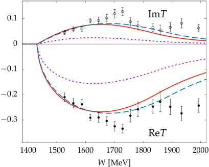
Figure 1: $T$-matrix amplitudes for the reaction $KN\to KN$ in the $S_{01}$ partial wave for different bag radii and interaction strengths. (See text for curve assignments.) Experimental data are from SAID .

Using our choice of $R=0.83$ fm and $f_{\pi}=73$ MeV, as well as the coupling constants predicted by the quark model (table 5), we underestimate the experimental $KN$ amplitudes (fig. 1, short dashes). Multiplying the coupling constants by a renormalization factor $f_{u}=1.35$ we are able to reproduce the amplitudes at low and intermediate energies (solid line). The agreement is improved if we choose a slightly smaller bag radius, $R=0.78$ fm, and $f_{u}=1.30$ (dashes).

In the following calculation we use the form and the renormalization factor derived above; we retain our standard choice of the bag radius, $R=0.83$ fm, which, as we see in the following, yields the most consistent results in other sectors.

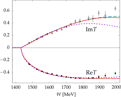
Figure 2: Same as fig. 1, but for the $S_{11}$ partial wave.

In the isospin $I=1$ channel (fig. 2) the contact interaction is present and dominates the amplitude; the exchange potential is relatively small and has the opposite sign with respect to the $I=0$ case as well as with respect to the contact potential. We obtain a good agreement with the contact potential alone using the rather standard choice of $R=0.83$ fm and the experimental value $f_{\pi}=93$ MeV (dashes); adding the exchange potential the experimental data are equally well reproduced by taking $R=0.90$ fm and $f_{\pi}=85$ MeV (solid line). Similarly as in the $I=0$ case the data support bag radii close to those used to describe baryons. Larger radii, e.g. $R=1$ fm (short dashes), underestimate the Im$T$ part of the amplitude at higher $W$.

3.2 Dynamically generated $\Lambda(1405)$

Switching to the strangeness $S=-1$ sector, we first consider the case with no bare three-quark states. We solve the LSE (8) by using two channels, $\pi\Sigma$ and $\bar{K}N$, and assuming only contact interaction. We first use our standard choice of model parameters, $R=0.83$ fm and $f_{\pi}=73$ MeV. The position of the pole in the complex $W$ plane is calculated by using the Laurent-Pietarinen expansion L+P2013 ; L+P2014 ; L+P2015 . We obtain two poles: the upper pole very close to the $KN$ threshold and the lower one approaching the $\pi\Sigma$ threshold (table 1). Reducing the strength of the interaction by assuming slightly larger values for $f_{\pi}$, the mass of the lower pole rises to the nominal value given in PDG2020 , while the upper pole remains close to the $KN$ threshold. The width of the upper pole is consistent with the PDG value while the width of the lower pole seems to be underestimated by a factor of two. Let us note that in this case there is only one pole of the $K$ matrix, which lies close to its nominal Breit-Wigner mass (fig. 3).

If we further reduce the strength of the contact term, only one pole remains, with a mass slightly below the $KN$ threshold. This pole corresponds to the pole found in the same model in Ref. Thomas85 .

Table 1: The pole parameters obtained from the $S_{01}$ partial wave amplitudes in the $\pi\Sigma$ channel using the Laurent-Pietarinen expansion

resonance	Re$W$	$-2{\rm Im}W$	Module	$R$	$f_{\pi}$
	[MeV]	[MeV]	[MeV]	[fm]	[MeV]
$\Lambda(1380)$	1348	33	16	0.83	73
	1378	48	20	0.83	78
$\Lambda(1405)$	1433	20	1	0.83	73
	1435	18	1	0.83	78
	1430	10	3	1.00	100
	1428	14	5	1.10	93

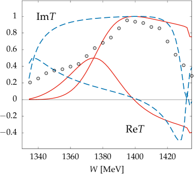
Figure 3: The real and imaginary part of the $\pi\Sigma\to\pi\Sigma$ amplitude for $R=0.83$ fm and $f_{\pi}=78$ MeV (solid line), and for $R=1.1$ fm and $f_{\pi}=93$ MeV (dashes). Since below the $KN$ threshold only the $\pi\Sigma$ channel is open, Im$T$ is proportional to the invariant mass distribution of $\pi\Sigma$ pairs and is compared to the experimental points in Hemingway1985 .

Our results with smaller values of $R$ and $f_{\pi}$ are consistent with the predictions of the chiral unitary theory and seem to suggest that no bare three-quark states are needed to reproduce at least the lowest resonance in the $S_{01}$ partial wave. There is a caveat, however: if we want to reproduce the subsequent two $I=0$ resonances, the $\Lambda(1670)$ and $\Lambda(1800)$, we have to assume the existence of at least two genuine quark model states. Yet carrying out such a calculation we find that the required strength of the contact potential, necessary to support dynamically generated resonances below the $KN$ threshold, is much too large in order to reproduce the experimental scattering amplitudes in the region of the upper two $S_{01}$ resonances. In fact, Kamano et al. Kamano14 , who have done a rather extensive analysis of the partial-wave amplitudes for $K^{-}p$ scattering, have found a better agreement for the $S_{01}$ case without including the contact interaction.

3.3 Including bare three-quark states in the $S_{01}$ partial wave

For the $S_{01}$ partial wave we include the quark model states corresponding to the lowest three resonances, assuming one quark is promoted from the $s$ orbit to the $p_{1/2}$ orbit. We further assume one singlet configuration, that can be identified as the $\Lambda(1405)$, and two octet configurations, with internal spin $S={1\over 2}$ (doublet) and $S={3\over 2}$ (quadruplet) that can be identified as the $\Lambda(1670)$ and $\Lambda(1800)$. We use the $j$-$j$ coupling scheme identical to the one used for the non-strange $S_{11}$ resonances EPJ2011 . The bare mass of the singlet state has been fixed by requiring that a pole of the $K$ matrix lies at $W=1405$ MeV; the masses and a possible mixing angle of the bare octet states are free parameters.

We consider four channels: $\pi\Sigma$, $\bar{K}N$, $\eta\Lambda$, and $K\Xi$, and assume that the physical $\eta(548)$ implies $\eta=\eta_{8}\cos\theta_{P}-\eta_{1}\sin\theta_{P}$ with $\theta_{P}=-11.3^{\circ}$ PDG2020 . We are not interested in obtaining the best fit to the experimental amplitudes but rather to investigate to what extent the quark model is able to reproduce the main features of the scattering amplitudes. We therefore retain the quark-model values in table 4 for the first two channels, as well as for $\eta_{8}\Lambda\Lambda^{*}_{1}$. The measured cross-section for $K^{-}+p\to\eta\Lambda$ BNL imposes a rather strong constraint on $\eta\Lambda$ coupling to the octet $\Lambda^{*}_{8}$ and suggests a much smaller value for this coupling than the one predicted by the quark model; similarly we take smaller values for $g_{K\Xi\Lambda^{*}}$. We further assume our standard choice for the bag radius of $R=0.83$ fm for all pertinent baryons as well as for the decay constants $f_{\pi}=f_{\eta}=f_{K}=73$ MeV.

The background potential (and the kernel entering the LSE) consists of the $u$-channel exchange potential and the contact potential. Based on our discussion of $KN$ scattering for $I=0$ we keep beside the nonstrange baryons in table 6 only the $\Lambda^{*}$ as the exchange baryons with $S=-1$, and further assume a renormalization of the coupling constants in table 5 by a factor of $f_{u}=1.35$ for the $\bar{K}N$ as well as for the $\pi\Sigma$ channels. We control the strength of the contact term by adjusting the value of $f_{\pi}$ which is allowed to differ from the (fixed) value used in the meson-baryon interaction.

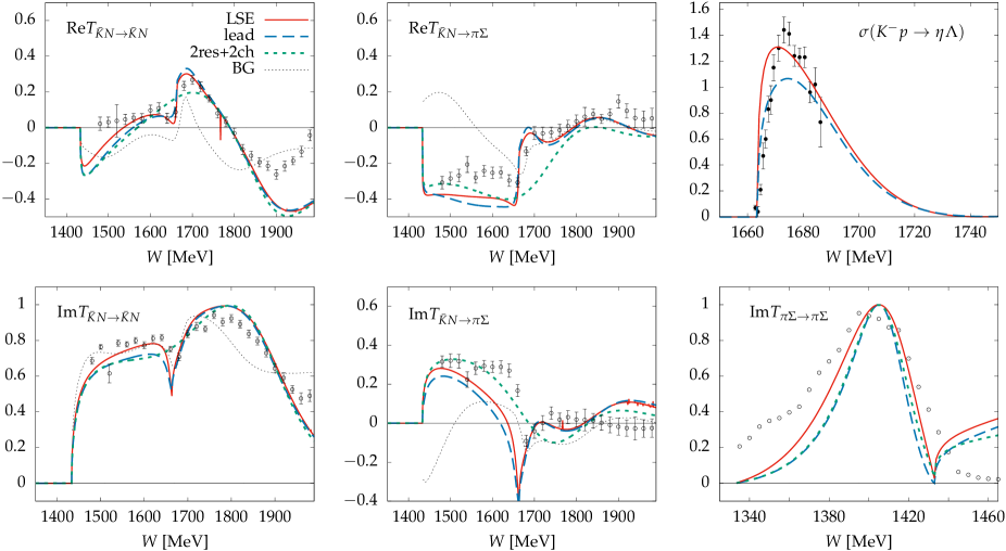
Figure 4: The scattering amplitudes for reactions $\bar{K}N\to\bar{K}N$, $\bar{K}N\to\pi\Sigma$ and $\pi\Sigma\to\pi\Sigma$, and the cross-section for $K^{-}p\to\eta\Lambda$. “LSE” stands for solving the Lippmann-Schwinger equation, “lead” for the leading order, “2res+2ch” for only two channels and two resonances, “BG” is the Bonn-Gatchina solution Sarantsev19a . Experimental data from Manley13a for the amplitudes, BNL for the cross-section and Hemingway1985 for the invariant mass distribution.

As we have mentioned in the previous section, using the strength of the contact interaction that produces two poles below the $KN$ threshold results in the scattering amplitudes which strongly disagree with experiment. Only when the contact interaction is reduced to less than 10 % of that strength, the calculated amplitudes start to exhibit the typical pattern seen in the $\bar{K}N\to\bar{K}N$ and $\bar{K}N\to\pi\Sigma$ reactions. In fact, we have found the best agreement by putting the strength of the contact interaction to zero. This finding agrees with the results of the analysis of Kamano et al. (Kamano14 , Model A) who find a good overall agreement in this partial wave without including the contact interaction.

The results for scattering in the $S_{01}$ partial wave are displayed in fig. 4; the real and the imaginary parts of the $T$ matrix are compared to the results for $\bar{K}N\to\bar{K}N$ and $\bar{K}N\to\pi\Sigma$ from the single-energy partial-wave analysis Manley13a , as well as to the analysis of the Bonn-Gatchina group Sarantsev19a . Furthermore, the calculated cross-section for $K^{-}p\to\eta\Lambda$ is compared to the measured one BNL , and in addition, the imaginary part of $T(\pi\Sigma\to\pi\Sigma)$ is confronted with the $\pi\Sigma$ invariant mass spectrum Hemingway1985 . The bare mases used in the calculation are displayed in table 2; we assume no mixing between the two bare octet configurations, the $K\Xi$ couplings to all $\Lambda^{*}$ are reduced to 30 % of the QM value, while the $\eta_{8}\Lambda$ coupling to the octet $\Lambda^{*}$ even to 10 % of the QM value.

Table 2: The pole parameters obtained from the $S_{01}$ partial wave amplitudes in different channels using the Laurent-Pietarinen expansion; “lead” stands for the solution in the leading order; $m^{0}$ is the bare quark mass.

res.	chan.	Re$W$	$-2{\rm Im}W$	modul.	QM	$m^{0}$
		[MeV]	[MeV]	[MeV]	assign.	[MeV]
$\Lambda(1405)$	$\pi\Sigma$-$\pi\Sigma$	1417	30	14.4	${}^{2}1[70]$	1667
	(lead)	1413	26	13.1		1637
$\Lambda(1670)$	$\pi\Sigma$-$\pi\Sigma$	1667	29	7.3	${}^{4}8[70]$	1720
	(lead)	1669	32	9.5		1713
	$\bar{K}N$-$\bar{K}N$	1664	26	3.8
	(lead)	1664	34	4.8
	$\bar{K}N$-$\pi\Sigma$	1664	36	6.7
	(lead)	1666	43	9.0
$\Lambda(1800)$	$\bar{K}N$-$\bar{K}N$	1885	341	157	${}^{2}8[70]$	1746
	(lead)	1882	358	204		1749
	$\bar{K}N$-$\pi\Sigma$	1814	198	26
	(lead)	1790	207	31

Our calculation shows that the scattering amplitudes are dominated by the resonant terms and that the background potential plays a rather minor role. Furthermore, evaluating the amplitudes without solving the LSE, i.e. by keeping only the leading terms in Eqs. (7) and (8), and readjusting sightly the bare masses, the result of the full calculation changes only insignificantly (long dashes vs. solid line for the LSE in fig. 4).

We have performed the Laurent-Pietarinen expansion to determine the positions of the poles in the complex $W$ plane (table 2). The mass and the width of the lowest pole determined in the $\pi\Sigma$ channel are consistent with the PDG values for the $\Lambda(1405)$. The values for the second pole are calculated from the amplitudes for three different reactions, and all three give values consistent with the PDG result for the $\Lambda(1670)$. For the third pole the values from $\bar{K}N$-$\bar{K}N$ differ more substantially from the preferred PDG values, while the results for $\bar{K}N$-$\pi\Sigma$ agree well with the PDG values. These results change only marginally in the leading order.

In our approach only the $\pi\Sigma$ channel provides the information about the poles below the $KN$ threshold. Still, some information can be obtained also from the $\bar{K}N$ amplitude by expanding the $T$ matrix for small $k$ Kamano15 , $T=k\left(a^{-1}-ik+{1\over 2}r_{e}k^{2}\right)^{-1}$, which yields the scattering length $a_{0\,\mathrm{LSE}}=(-1.32+i\,1.00)$ fm and $a_{0\,\mathrm{lead}}=(-1.42+i\,0.71)$ fm, and the pole at $W_{\mathrm{LSE}}=(1434.8-i\,22.1)$ MeV and at $W_{\mathrm{lead}}=(1425.6-i\,21.5)$ MeV. Both values of the scattering length are inside the allowed region established in Ref. Doering11 and deduced from the SIDDHARTA measurements SIDDHARTA . While the width is consistent with the values in table 2 for the $\pi\Sigma$ channel, the mass comes much too close to the threshold value in this approximation.

Next we have considered the case with only two channels, $\pi\Sigma$ and $\bar{K}N$, and two bare three-quark states, the $\Lambda_{1}^{*}$ and ${}^{2}\Lambda_{8}^{*}$. Again we obtain a similar behaviour of amplitudes as in the full calculation in a wide energy range except for the interval in the vicinity of the second resonance $\Lambda(1670)$, neglected in this approximation.

We shall discuss the nature of the lowest resonance in Sec. 4.

Let us comment here on similar calculations in the framework of the same model in Refs. Thomas85 and Fink90 where the contact interaction as well as the bare three-quark state were included. In the former work a single pole below the $KN$ threshold was found, while in the latter two poles were found in the $\pi\Sigma$ channel, one close to the $KN$ and another close to the $\pi\Sigma$ threshold. In both approaches the choice of the bag radius and pion decay constant resulted in a rather weak strength of the contact interaction as well as of the quark-meson interaction, hence the resonances below the $KN$ threshold were generated through the dynamical mechanism discussed in the previous subsection.

3.4 Including three-quark states in the $S_{11}$ partial wave

In the $S_{11}$ partial wave we include five channels, $\pi\Sigma$, $\bar{K}N$, $\pi\Lambda$, $K\Xi$ and $\eta\Sigma$, and two bare quark state corresponding to ${}^{2}\Sigma^{*}_{8}$ and ${}^{4}\Sigma^{*}_{8}$. The inclusion of the contact interaction turns out to be mandatory here. With our standard choice for $R$ and $f_{\pi}$ controlling the meson-baryon interaction, a satisfactory agreement — at least for $W$ below 1750 MeV — is reached by using $f_{\pi}=128$ MeV for the contact interaction. In addition, we assume that the strength of the $\pi\Sigma\Sigma^{*}_{8}$ coupling constant is reduced by 30 % with respect to the quark-model value, and a mixing angle of $20^{\circ}$ is used already at the level of bare ${}^{2}\Sigma^{*}_{8}$ and ${}^{4}\Sigma^{*}_{8}$ states. For the channels $\bar{K}N$, $\pi\Lambda$, $K\Xi$ we fix the coupling constants to their quark-model values, while for the $\eta\Sigma$ channel we use the same prescription as for the $\eta\Lambda$ channel in the $S_{01}$ partial wave. The optimal masses of the bare quark states remain close to their nominal values 1750 MeV and 1900 MeV, i.e. $m(^{2}\Sigma^{*}_{8})=1750$ MeV and $m(^{4}\Sigma^{*}_{8})=1876$ MeV.

Figure 5: Amplitudes for $I=1$: the solid line represents the full solution, the dashes the leading order solution, and the short dashes the full solution with only three channels. The tiny dashes and the experimental points as in fig. 4.

In fig. 5 we compare the full calculation by solving LSE with all five channels, the full calculation which includes only $\pi\Sigma$, $\bar{K}N$, $\pi\Lambda$ channels, and the calculation in the leading order (without solving LSE). As expected, the first three channels dominate at lower $W$, but in contrast to the $S_{01}$ partial wave, the leading order solution differs considerably from the full solution as a consequence of a much stronger potential that enters the LSE.

The positions of the poles in the complex $W$ plane are displayed in table 3. While the lower pole is located at too large Re$W$ and too small Im$W$ compared to the PDG values, the upper pole is better reproduced in the case of five channels. The scattering length in the case of five (three) channels is $a_{1}=(0.54-i\,0.39)$ fm ($a_{1}=(0.52-i\,0.41)$ fm); while the real parts are well within the allowed region advocated in Ref. Doering11 , the imaginary parts seems to be slightly too low.

Table 3: The pole parameters obtained in the $S_{11}$ partial wave by using five or three channels.

res.	chan.	Re$W$	$-2{\rm Im}W$	modul.	QM	$m^{0}$
react.		[MeV]	[MeV]	[MeV]	assign.	[MeV]
$\Sigma(1750)$	5 & 3				${}^{2}8[70]$	1750
$\bar{K}N$-$\bar{K}N$	5	1738	48	1.7
	3	1784	75	7.8
$\bar{K}N$-$\pi\Sigma$	5	1786	54	4.8
	3	1785	75	13.8
$\bar{K}N$-$\pi\Lambda$	5	1788	49	2.1
	3	1785	73	5.1
$\Sigma(1900)$	5 & 3				${}^{4}8[70]$	1876
$\bar{K}N$-$\bar{K}N$	5	1924	96	18.1
	3	1914	61	21.5
$\bar{K}N$-$\pi\Sigma$	5	1925	123	10.7
	3	1914	60	3.0
$\bar{K}N$-$\pi\Lambda$	5	1924	81	10.3
	3	1914	61	12.9

From both partial waves we can construct the amplitudes for the decay of the $\Lambda(1405)$ into $\Sigma^{+}\pi^{-}$, $\Sigma^{-}\pi^{+}$, and $\Sigma^{0}\pi^{0}$, and compare them to those extracted in the reactions $p+p\to\Sigma^{\pm}+\pi^{\mp}+K^{+}+p$ by the HADES collaboration HADES13 , and $\gamma+p\to K^{+}+\Sigma+\pi$ by the CLAS Collaboration CLAS13 . The corresponding $|T_{\Sigma^{-}\pi^{+}}|^{2}$, $|T_{\Sigma^{0}\pi^{0}}|^{2}$ and $|T_{\Sigma^{+}\pi^{-}}|^{2}$ can be straightforwardly expressed in terms of the $T$-matrix amplitudes for the $S_{01}$ and $S_{11}$ partial waves (assuming no contribution from $I=2$) and related to the cross-section for the above reactions. We shall not attempt to write down the explicit expression for the cross-section but rather compare the qualitative behaviour of $|T_{\Sigma\pi}|^{2}$ with the mass distribution of the model by Bayar et al. Bayar18 based on HADES data. Comparing our fig. 6 with their fig. 6 we notice that the positions of peaks for the $\pi^{+}$, $\pi^{0}$ and $\pi^{-}$ distributions are similar, also the $\pi^{+}$ distribution is dominant in both cases. Let us note that below the $KN$ threshold the $\pi^{0}$ distribution is one third of the Im$T_{\pi\Sigma-\pi\Sigma}$ amplitude and is in our case peaked around the nominal mass of the resonance at $m=1405$ MeV which corresponds to one of the free parameters in our model. Such a value is supported also by the analysis of HADES data by Hassanvand et al. Hassanvand13 . A similar comparison of mass distributions in different channels to those obtained by Ulf15 and Mari21 (both based on CLAS data), is less conclusive.

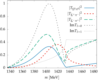
Figure 6: The (squared) $T$ amplitudes for $\Lambda^{*}\to\Sigma\pi$ as function of the invariant mass $m$.

4 The structure of the resonances

4.1 Evolution of poles in the complex energy plane

In order to obtain a deeper insight into the mechanism of resonance formation in the presence of genuine three-quark states in the $S_{01}$ partial wave we follow the evolution of the $S$-matrix poles in the complex energy plane as a function of the interaction strength by performing the Laurent-Pietarinen expansion. We start from the genuine three-quark states and calculate the scattering amplitudes by gradually increasing the meson-baryon coupling constants in all channels by a factor $g,\>0<g\leq 1$, to finally reach the physical values used in the previous Section. This approach has been used in our previous work PRC2018 ; PRC2019 to show that the Roper resonance evolves from the genuine three-quark state, while the $\Delta(1600)$ emerges as a dynamically generated state.

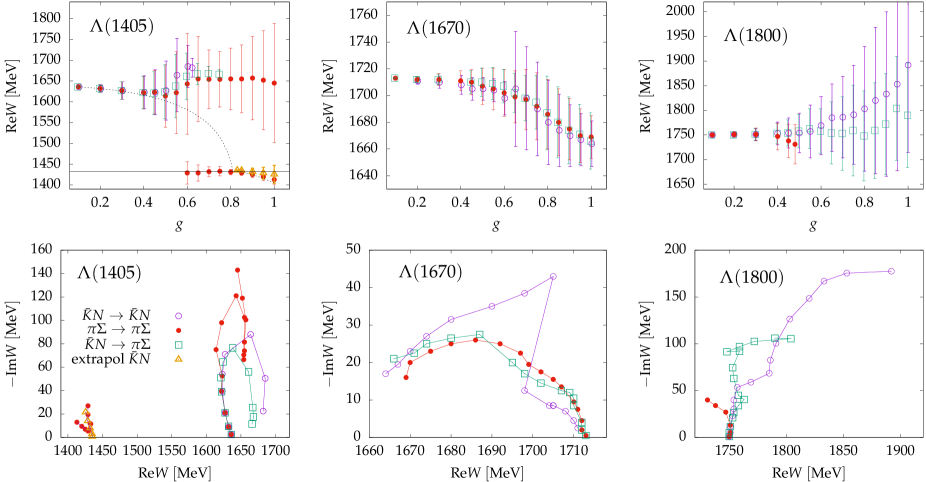
Figure 7: Evolution of poles of the three resonant states as a function of interaction strength (top panels) with error bars corresponding to $\pm|\mathrm{Im}W|$, and in the complex $W$ plane (bottom panels). The full circles correspond to $\pi\Sigma\to\pi\Sigma$, the empty circles to $\bar{K}N\to\bar{K}N$, squares to $\bar{K}N\to\pi\Sigma$, and triangles to the $\bar{K}N\to\bar{K}N$ amplitudes extrapolated below the threshold.

In the present case we deal with an evolution of three resonances that lie relatively close to each other and strongly mix, particularly in the region of intermediate coupling strengths. This represent a serious difficulty in identifying the poles belonging to individual resonances, which may overlap or even cross. Furthermore, the presence of the $KN$ and $\eta\Lambda$ thresholds may strongly influence the poles in their vicinity. It turns out that the procedure is more stable if one uses the leading solution due to smaller widths of the resonances. Yet the final solution stays close to the full calculation (see table 2), so the conclusion should be valid also for the full solution.

The evolution for the reactions $\bar{K}N\to\bar{K}N$, $\bar{K}N\to\pi\Sigma$ and $\pi\Sigma\to\pi\Sigma$ is shown in fig. 7. We do not show $\bar{K}N\to\eta\Lambda$ since the relevant pole lies very close to the threshold and its determination is less reliable.

The evolution of the lower resonance (left panels) starts with the three-quark singlet configuration. The evolution for $\bar{K}N\to\bar{K}N$ and $\bar{K}N\to\pi\Sigma$ stops at $g=0.6$ and $g=0.7$, respectively, as the widths and moduli vanish. This does not happen in the $\pi\Sigma$ channel, the evolution rather continues away from the real axis. Beyond $g>0.5$ another branch appears and evolves toward the pole that can be identified as $\Lambda(1405)$; at larger $g$ this branch can also be obtained by using the small-$k$ expansion for $T_{\bar{K}N\,\bar{K}N}$. From our analysis it is unclear whether (i) this branch emerges at the threshold and evolves independently of the upper branch or (ii) it smoothly evolves from the genuine three-quark state, in which case there would exist a bifurcation for $\pi\Sigma\to\pi\Sigma$ in the intermediate regime of $g$. Though the curves presented in fig. 7 favor the first possibility, we should mention that the determination of the pole in the vicinity of the threshold is unreliable and its position very close to the threshold may be an artifact. Plotting the (real) pole of the $K$ matrix as a function of $g$ supports the second possibility since it exhibits a rather rapid transition from the bare value to values below the threshold.

The branch above $g=0.80$, where the mass of the pole starts moving away from the threshold value, has a clear physical interpretation, which will be discussed in the following.

The evolution of the middle resonance (central panels) starting with the three-quark octet configuration with spin $S={\textstyle{\frac{3}{2}}}$ is smooth except around $g=0.6$ in the $\bar{K}N$ channel where the pole pertaining to the $\Lambda(1405)$ (left panel) in this channel disappears. All three evolutions end up at the pole which can unmistakably be attributed to the physical $\Lambda(1670)$ resonance, and confirm the assignment given in table 2.

The evolution of the upper resonance (right panels) starting with the three-quark octet configuration with spin $S={\textstyle{\frac{1}{2}}}$ is smooth and in $\bar{K}N\to\bar{K}N$ and $\bar{K}N\to\pi\Sigma$ evolves to the resonance that can be identified as $\Lambda(1800)$, though in the $\bar{K}N$ channel it terminates at too large Re$W$ and Im$W$. The $\pi\Sigma$ system is only weakly coupled to the bare state and above $g=0.5$ becomes too weak to be detected.

4.2 Structure of the $\Lambda(1405)$ resonance

Let us observe the evolution of the $\bar{K}N$ channel below the $KN$ threshold as $W$ approaches $m_{\Lambda}$, the lowest pole of the $K$ matrix. If we normalize the corresponding channel state (1) by inverting the norm (4) and taking into account that both terms are dominated by $c_{\bar{K}N\Lambda^{*}}\propto(W-m_{\Lambda})^{-1}$, the channel state can be cast in the form

$$|\Psi_{\bar{K}N}\rangle = \sqrt{Z}\left(|\Phi^{0}_{\Lambda^{*}}\rangle+\int{dk\,\mathcal{V}_{\bar{K}N\Lambda^{*}}(k)\over\omega_{k}+E_{N}(k)-W}\left[a_{K}^{\dagger}(k)|\Phi_{N}\rangle\right]\right.$$ (17)

$$+ \left.\int{dk^{\pi}\,\mathcal{V}_{\pi\Sigma\Lambda^{*}}(k^{\pi})\over\omega_{k}^{\pi}+E_{\Sigma}(k^{\pi})-W}\left[a_{\pi}^{\dagger}(k^{\pi})|\Phi_{\Sigma}\rangle\right]+\ldots\right)\,,$$

where $k$ refers to the kaon momentum. The terms involving the $\eta\Lambda$ and $K\Xi$ components, as well as the octet admixtures to singlet three-quark state, are small and will be neglected in the following. The norm then reads

$$Z^{-1}=1+\int{dk\,\mathcal{V}^{2}_{\bar{K}N\Lambda^{*}}(k)\over(\omega_{k}+E_{N}(k)-W)^{2}}-{d\over dW}\Sigma_{\pi\Sigma}(W)\,.$$ (18)

We notice that for $W$ close to the threshold, the second term in Eq. (18) strongly dominates and the system is very loosely bound (see fig. 8), however, at the physical value of the coupling strength it becomes comparable to the weight of the bare three-quark component (see fig. 9). The contribution from the $\pi\Sigma$ component (expressed in terms of the derivative of the self-energy) remains very small. On the other hand, the contribution to the energy is dominated by both the $\bar{K}N$ as well as the $\pi\Sigma$ self-energies, which are responsible to push the mass of the physical $\Lambda(1405)$ below the $KN$ threshold; this mechanism is similar to the one proposed by Arima et al. Arima94 .

Our model therefore confirms the picture in which the $\Lambda(1405)$ is predominantly a $\bar{K}N$ molecular state; however, in our model the binding mechanism is not the contact interaction that would generate attraction between the (anti)kaon and the nucleon but rather the $\bar{K}N\Lambda^{*}$ interaction which implies the presence of a bare three-quark configuration with the quantum numbers of the resonance; the presence of the $\pi\Sigma$ channel is also necessary to ensure the binding. Let us mention that the $\Lambda(1405)$ is not a Feshbach resonance since the energy of the state (17) alone is well above the $KN$ threshold.

A similar model with a bare state and the kaon cloud around the nucleon was proposed long ago by Thomas et al. Thomas85 in the framework of the same model; in our approach we have extended the model by inclusion of other channels and resonances, but also showing that the presence of the contact term is not mandatory. Our picture of the resonance can also be related to the state found on the lattice Leinweber12 ; Leinweber15 and interpreted in the framework of Hamiltonian effective theory Leinweber18 .

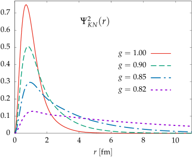
Figure 8: Kaon probability density for different relative coupling strengths.

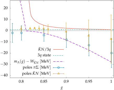
Figure 9: Evolution of the $\Lambda(1405)$ (Breit-Wigner) mass (dashes), pole mass and width (error bars) from the $\pi\Sigma$ (circles) and $\bar{K}N$ (triangles) channels, and the weight of the $\bar{K}N$ component (solid line) normalized such that the weight of the three-quark state is equal one (short dashes). Masses are measured with respect to the $KN$ threshold.

5 Conclusion

As we have shown in Sec. 3 our model is able to generate a ${\textstyle{\frac{1}{2}}}^{-}$ resonance — or even two resonances — below the $KN$ threshold either as a molecular state or a genuine three-quark state dressed with baryon-meson pairs. We believe that in order to give credence to either of the two approaches it is important to carry out the calculation of the $S_{01}$ partial wave amplitudes in the relevant channels by treating all three resonances in a unified framework. The main and, admittedly, rather surprising, conclusion of our investigation is that the scattering amplitudes are dominated by the quark degrees of freedom rather than by non-linear dynamics of the baryon-meson systems. By using our standard choice of model parameters which had successfully reproduced the scattering as well as electroproduction amplitudes in the nonstrange sector we have been able to obtain a satisfactory result already in the leading order; solving the LSE only marginally improves the results. Furthermore, as in the calculation of Kamano et al. Kamano14 , we have found that including the contact interaction does not improve the results. Our results therefore confirm that the main mechanism to lower the mass of the $\Lambda(1405)$ by $\approx 250$ MeV with respect to its bare value is the one suggested by Arima et al. Arima94 , that is, the attractive self-energy term in the $\pi\Sigma$ and $\bar{K}N$ channels, with the latter term being strongly enhanced due to the presence of the $KN$ threshold. Nonetheless, even without including the contact interaction, we have been able to observe the formation of the $\bar{K}N$ molecular state. By gradually increasing the strength of all meson-baryon couplings, a resonant state, strongly dominated by a weakly bound $\bar{K}N$ component and an almost negligible admixture of the bare three-quark and $\pi\Sigma$ components, emerges slightly below the $KN$ threshold. At the physical strength, at which this state can be identified with the $\Lambda(1405)$ resonance, the molecular component becomes weaker but still dominates over the bare quark state which, in turn, is dominated by the singlet component. There is, however, an important difference between our state and the molecular state of the chiral unitary approach; in our approach the attraction is generated through the $\bar{K}N\Lambda^{*}$ coupling and therefore the presence of the singlet state is mandatory.

Regarding the two higher lying resonances, the $\Lambda(1670)$ is well reproduced and assigned to $S={3\over 2}$; with the $\Lambda(1800)$ there remains some ambiguity about the determination of its mass in different channels, which signals that our model becomes less reliable at higher $W$.

In the $S_{11}$ partial wave it turns out that the inclusion of the contact interaction is important; we reproduce reasonably well the scattering amplitudes in the energy range from the threshold up to around 1750 MeV using either all five channels or solely the $\pi\Sigma$, $\bar{K}N$, and $\pi\Lambda$ channels.

Appendix A The Cloudy Bag Model meson-quark vertices and coupling constants

The $s$-wave quark-meson vertices $\hat{V}(k)$ in Eq. (11) are evaluated in the Cloudy Bag Model assuming that in the resonant state one of the three quarks is excited from the $1s$ state to the $1p_{1/2}$ state.

For the quark part of the quark-pion, quark-eta meson and quark-kaon interaction we obtain

$$\hat{V}^{\pi}_{l=0,t}(k) = V^{\pi}(k)\sum_{i=1}^{3}\tau_{t}(i)\,\mathcal{P}_{sp}(i)\,,$$ (19)

$$\hat{V}^{\eta}(k) = V^{\eta}(k)\sum_{i=1}^{3}\lambda_{8}(i)\,\mathcal{P}_{sp}(i)\,,$$ (20)

$$\hat{V}^{K}_{t}(k) = V^{K}(k)$$ (21)

Here $\mathcal{P}_{sp}=\sum_{m_{j}}|sm_{j}\rangle\langle p_{1/2}m_{j}|$, $\omega_{s}=2.043$, $\omega_{p_{1/2}}=3.811$, $X(K^{0})=-(\lambda_{6}-i\lambda_{7})/\sqrt{2}$, $X(\bar{K}^{0})=-(\lambda_{6}+i\lambda_{7})/\sqrt{2}$, $X(K^{+})=-(\lambda_{4}-i\lambda_{5})/\sqrt{2}$, $X(K^{-})=(\lambda_{4}+i\lambda_{5})/\sqrt{2}$. Assuming $f_{\eta}=f_{K}=f_{\pi}$, the form-factors of the surface part and of the volume part take the form

$$V^{\pi}_{S}(k) = V^{\eta}_{S}(k)=V^{K}_{S}(k)$$

$$= {1\over 2f_{\pi}}\sqrt{\omega_{p_{1/2}}\omega_{s}\over(\omega_{p_{1/2}}+1)(\omega_{s}-1)}\,{1\over 2\pi}\,{k^{2}\over\sqrt{\omega_{k}}}\,{j_{0}(kR)\over kR}\,,$$

$$V_{V}(k) = \left[{\omega_{s}\over R}-{\omega_{p1/2}\over R}+\omega_{M}(k)\right]$$ (22)

$$\times \int_{0}^{R}dr\,r^{2}[u_{s}(r)u_{p}(r)+v_{s}(r)v_{p}(r)]j_{0}(kr)\,.$$

For the physical $\eta$ we assume $\eta=\cos\theta_{P}\eta_{8}-\sin\theta_{P}\eta_{1}$, for the singlet $\eta_{1}$ $\lambda_{8}$ is replaced by $\lambda_{1}$ in Eq. (20).

The coupling constants for the $s$-channel exchange potential are collected in table 4, those for the $u$-channel exchange potential involving strange baryons in table 5, and for exchange of nonstrange baryons in table 6.

Table 4: Reduced $X^{*}\to MB$ matrix elements

$X^{*}/BM$	$\pi\Sigma$	$\pi\Lambda$	$\eta_{1}\Lambda$	$\eta_{8}\Lambda$	$\eta_{1}\Sigma$	$\eta_{8}\Sigma$	$\bar{K}N$	$K\Xi$
$\Lambda^{*}_{1}$	$\sqrt{3}$	0	0	$-1$	0	0	$\sqrt{2}$	$\sqrt{2}$
$\Lambda^{*}_{28}$	$-{\sqrt{3}\over 3}$	0	${2\sqrt{2}\over 3}$	$-{1\over 3}$	0	0	$\sqrt{2}$	$-{2\sqrt{2}\over 3}$
$\Lambda^{*}_{48}$	${2\sqrt{3}\over 3}$	0	${2\sqrt{2}\over 3}$	${2\over 3}$	0	0	$0$	$-{2\sqrt{2}\over 3}$
$\Sigma^{*}_{28}$	$-{5\over 3}\sqrt{2\over 3}$	$-{1\over 3}$	0	0	${2\sqrt{2}\over 3}$	${1\over 3}$	$-{1\over 3}\sqrt{2\over 3}$	${4\over 3}\sqrt{2\over 3}$
$\Sigma^{*}_{48}$	$-{2\over 3}\sqrt{2\over 3}$	${2\over 3}$	0	0	${2\sqrt{2}\over 3}$	$-{2\over 3}$	$-{4\over 3}\sqrt{2\over 3}$	$-{2\over 3}\sqrt{2\over 3}$

Table 5: Reduced $B\to MX^{*}$ matrix elements

$X^{*}/BM$	$\Sigma\pi$	$\Lambda\pi$	$\Lambda\eta_{1}$	$\Lambda\eta_{8}$	$\Sigma\eta_{1}$	$\Sigma\eta_{8}$	$NK$	$\Xi\bar{K}$
$\Lambda^{*}_{1}$	$1$	0	0	$-1$	0	0	1	1
$\Lambda^{*}_{28}$	${1\over 3}$	0	${2\sqrt{2}\over 3}$	$-{1\over 3}$	0	0	1	$-{2\over 3}$
$\Lambda^{*}_{48}$	$-{2\over 3}$	0	${2\sqrt{2}\over 3}$	${2\over 3}$	0	0	0	$-{2\over 3}$
$\Sigma^{*}_{28}$	$-{5\over 3}\sqrt{2\over 3}$	${\sqrt{3}\over 3}$	0	0	${2\sqrt{2}\over 3}$	${1\over 3}$	$-{1\over 3}$	${4\over 3}$
$\Sigma^{*}_{48}$	$-{2\over 3}\sqrt{2\over 3}$	$-{2\sqrt{3}\over 3}$	0	0	${2\sqrt{2}\over 3}$	$-{2\over 3}$	$-{4\over 3}$	$-{2\over 3}$

Table 6: Reduced $B\to MS^{*}$ matrix elements for non-strange $s$-wave resonances

$S^{*}/BM$	$\Sigma\bar{K}$	$N\pi$	$\Lambda\bar{K}$	$N\eta_{1}$	$N\eta_{8}$
$S11_{2}$	$-{1\over 3}\sqrt{2\over 3}$	$-{4\over 3}$	$-\sqrt{2}$	${2\sqrt{2}\over 3}$	${2\over 3}$
$S11_{4}$	$-{4\over 3}\sqrt{2\over 3}$	${2\over 3}$	0	${2\sqrt{2}\over 3}$	${2\over 3}$
$S31$	${2\over 3}\sqrt{2\over 3}$	${2\over 3}$	0	0

Appendix B Contact interaction

For the $s$-wave mesons the contact interaction can be cast in the form

$$V^{c}_{\alpha\beta}(k,k^{\prime}) = {g_{\alpha\beta}\over 2f^{2}_{\pi}}{kk^{\prime}\over 2\pi^{2}\sqrt{2\omega_{\alpha}(k)}\sqrt{2\omega_{\beta}(k^{\prime})}}$$

$$\kern-60.0pt\times[\omega_{\alpha}(k)+\omega_{\beta}(k^{\prime})]\int_{0}^{R}dr\,r^{2}[u_{s}^{2}(r)+v_{s}^{2}(r)]j_{0}(kr)j_{0}(k^{\prime}r)\,.$$

Here $g_{\alpha\beta}$ can be identified with $-2f_{\pi}^{2}\lambda^{I}_{\alpha\beta}$ of Thomas85 and ${\textstyle{\frac{1}{2}}}\mathcal{D}_{\alpha\beta}$ of Oset98 and are collected in table 7.

Table 7: $g_{\alpha\beta}$ for isospin 0 and 1.

$$I=0\qquad{\begin{array}[]{|c|c|cccc|}\hline\cr g_{\alpha\beta}&KN&\bar{K}N&\pi\Sigma&\eta\Lambda&K\Xi\\ \hline\cr KN&0&&&&\\ \hline\cr\bar{K}N&&{3\over 2}&{\sqrt{6}\over 4}&{3\over\sqrt{8}}&0\\ \pi\Sigma&&{\sqrt{6}\over 4}&2&0&{\sqrt{6}\over 4}\\ \eta\Lambda&&{3\over\sqrt{8}}&0&0&-{3\over\sqrt{8}}\\ K\Xi&&0&{\sqrt{6}\over 4}&-{3\over\sqrt{8}}&{3\over 2}\\ \hline\cr\end{array}}$$

$$I=1\qquad{\begin{array}[]{|c|c|ccccc|}\hline\cr g_{\alpha\beta}&KN&\bar{K}N&\pi\Sigma&\pi\Lambda&K\Xi&\eta\Sigma\\ \hline\cr KN&-1&&&&&\\ \hline\cr\bar{K}N&&{1\over 2}&{1\over 2}&-{\sqrt{6}\over 4}&0&-{\sqrt{6}\over 4}\\ \pi\Sigma&&{1\over 2}&1&0&1&0\\ \pi\Lambda&&-{\sqrt{6}\over 4}&0&0&-{\sqrt{6}\over 4}&0\\ K\Xi&&0&1&-{\sqrt{6}\over 4}&1&-{\sqrt{6}\over 4}\\ \eta\Sigma&&-{\sqrt{6}\over 4}&0&0&-{\sqrt{6}\over 4}&0\\ \hline\cr\end{array}}$$

Oset Oset98 has an opposite sign for $\bar{K}N\leftrightarrow\pi\Sigma$, which is compensated by changing the sign for $\Sigma^{*}\to\pi\Sigma$.

References

- (1) M. H. Alston, et al., Phys. Rev. Lett. 6, 698 (1961).
- (2) N. Isgur, G. Karl, Phys. Rev. D 18, 4187 (1978).
- (3) J. W. Darewych, R. Koniuk, N. Isgur, Phys. Rev. D 32, 1765 (1985).
- (4) S. Capstick, N. Isgur, Phys. Rev. D 34, 2809 (1986).
- (5) U. Löring, B. C. Metsch, H. R. Petry, Eur. Phys. J. A 10, 447 (2001).
- (6) T. Melde, W. Plessas, B. Sengl, Phys. Rev. D 77, 114002 (2008).
- (7) M. Arima, S. Matsui, K. Shimizu, Phys. Rev. C 49, 2831 (1994).
- (8) R. H. Dalitz, S. F. Tuan, Ann. Phys. 10, 307 (1960).
- (9) R. H. Dalitz, T. C. Wong, G. Rajasekaran, Phys. Rev. 153, 1617 (1967).
- (10) N. Kaiser, P. B. Siegel, W. Weise, Nucl. Phys. A 594, 325, (1995).
- (11) E. Oset, A. Ramos, Nucl. Phys. A 635, 99 (1998).
- (12) M. F. M. Lutz, E. E. Kolomeitsev, Nucl. Phys. A 700, 193 (2002).
- (13) J. A. Oller, U. G. Meissner, Phys. Lett. B 500, 263 (2001).
- (14) D. Jido, J. A. Oller, E. Oset, A. Ramos, U. G. Meissner, Nucl. Phys. A 725, 181 (2003).
- (15) T. Hyodo, S. I. Nam, D. Jido, A. Hosaka, Phys. Rev. C 68, 018201 (2003).
- (16) C. Garcia-Recio, J. Nieves, E. R. Arriola, M. J. Vicente Vacas, Phys. Rev. D 67, 076009 (2003).
- (17) T. Hyodo, W. Weise, Phys. Rev. C 77, 035204 (2008).
- (18) Y. Ikeda, T. Hyodo, W. Weise, Phys. Lett. B 706, 63 (2011).
- (19) Y. Ikeda, T. Hyodo, W. Weise, Nucl. Phys. A 881, 98 (2012).
- (20) Z.-H. Guo, J. A. Oller, Phys. Rev. C 87, 035202 (2013).
- (21) L. Roca, E. Oset, Eur. Phys. J. A 56, 56 (2020).
- (22) M. Mai, U.-G. Meißner, Eur. Phys. J. A 51, 30 (2015).
- (23) K. S. Myint, Y. Akaishi, M. Hassanvand, T. Yamazaki, Prog. Theor. Exp. Phys. 2018, 073D01 (2018).
- (24) A. W. Thomas, Adv. Nucl. Phys. 13, 1 (1984).
- (25) E. A. Veit, B. K. Jennings, R. C. Barrett, A. W. Thomas, Phys. Lett. B 137, 415 (1984).
- (26) E. A. Veit, B. K. Jennings, A. W. Thomas, R. C. Barrett, Phys. Rev. D 31, 1033 (1985).
- (27) B. K. Jennings, Phys. Lett. B 178, 229 (1986).
- (28) E. A. Veit, A. W. Thomas, B. K. Jennings, Phys. Rev. D 31, 2242 (1985).
- (29) B. J. Menadue, W. Kamleh, D. B. Leinweber, M. S. Mahbub, Phys. Rev. Lett. 108, 112001 (2012).
- (30) J. M. M. Hall, W. Kamleh, D. B. Leinweber, B. J. Menadue, B. J. Owen, A. W. Thomas, R. D. Young, Phys. Rev. Lett. 114, 132002 (2015).
- (31) Z.-W. Liu, J. M. M. Hall, D. B. Leinweber, A. W. Thomas, J.-J. Wu, Phys. Rev. D 95, 014506 (2017).
- (32) G. P. Engel, C. B. Lang, A. Schäfer, Phys. Rev. D 87, 034502 (2013).
- (33) P. Gubler, T.T. Takahashi, and M. Oka, Phys. Rev. D 94, 114518 (2016).
- (34) R. Pavao, P. Gubler, P. Fernandez-Soler, J. Nieves, M. Oka, T.T. Takahashi, Phys. Lett. B 829 136473, (2021).
- (35) H. Zhang, J. Tulpan, M. Shrestha, D. M. Manley, Phys.Rev. C 88, 035204 (2013).
- (36) H. Zhang, J. Tulpan, M. Shrestha, D. M. Manley, Phys.Rev. C 88, 035205 (2013).
- (37) H. Kamano, S. X. Nakamura, T. S. H. Lee, T. Sato, Phys. Rev. C 90, 065204 (2014).
- (38) M. Matveev, A. V. Sarantsev, V. A. Nikonov, A. V. Anisovich, U. Thoma, E. Klempt, Eur. Phys. J. A 55, 179 (2019).
- (39) A. V. Sarantsev, M. Matveev, V. A. Nikonov, A. V. Anisovich, U. Thoma, E. Klempt, Eur. Phys. J. A 55, 180 (2019).
- (40) H. Kamano, S. X. Nakamura, T. S. H. Lee, T. Sato, Phys. Rev. C 92, 025205 (2015).
- (41) A. V. Anisovich, A. V. Sarantsev, V. A. Nikonov, V. Burkert, R. A. Schumacher, U. Thoma, E. Klempt, Eur. Phys. J. A 56, 139 (2020).
- (42) C. Fernandez-Ramirez, I. V. Danilkin, V. Mathieu, A. P. Szczepaniak, Phys. Rev. D 93, 074015 (2016)
- (43) E. Klempt, V. Burkert, U. Thoma, L. Tiator, R. Workman, Eur. Phys. J. A 56, 261 (2020).
- (44) B. Golli, H. Osmanović, S. Širca, A. Švarc, Phys. Rev. C 97, 035204 (2018).
- (45) B. Golli, H. Osmanović, S. Širca, Phys. Rev. C 100, 035204 (2019).
- (46) B. Golli, S. Širca, Eur. Phys. J. A 38, 271 (2008).
- (47) B. Golli, S. Širca, M. Fiolhais, Eur. Phys. J. A 42, 185 (2009).
- (48) B. Golli, S. Širca, Eur. Phys. J. A 47, 61 (2011).
- (49) B. Golli, S. Širca, Eur. Phys. J. A 49, 111 (2013).
- (50) B. Golli, S. Širca, Eur. Phys. J. A 52, 279 (2016).
-
(51)
https://gwdac.phys.gwu.edu/analysis/kn_analysis.html. - (52) A. Švarc, M. Hadžimehmedović, H.Osmanović, J. Stahov, L. Tiator, R. L. Workman, Phys. Rev. C 88, 035206 (2013).
- (53) A. Švarc, M. Hadžimehmedović, R. Omerović, H. Osmanović, J. Stahov, Phys. Rev. C 89, 045205 (2014).
- (54) A. Švarc, M. Hadžimehmedović, H. Osmanović, J. Stahov, R. L. Workman, Phys. Rev. C 91, 015207 (2015).
- (55) P. A. Zyla et al. (Particle Data Group), Prog. Theor. Exp. Phys. 2020, 083C01 (2020).
- (56) R. J. Hemingway, Nucl. Phys. B 253, 742 (1985).
- (57) A. Starostin et al. (Crystal Ball Collaboration), Phys. Rev. C 64, 055205 (2001).
- (58) M. Döring, U.-G. Meissner, Phys. Lett. B 704, 663 (2011).
- (59) M. Bazzi et al. (SIDDHARTA Collaboration), Nucl. Phys. A 881, 88 (2012).
- (60) P.J. Fink, G. He, R. H. Landau, J.W. Schnick, Phys. Rev. C 41, 2720 (1990).
- (61) G. Agakishiev et al. (HADES Collaboration) Phys. Rev. C 87, 025201 (2013).
- (62) K. Moriya et al. (CLAS Collaboration), Phys. Rev. C 87, 035206 (2013).
- (63) M. Bayar, R. Pavao, S. Sakai, E. Oset, Phys. Rev. C 97, 035203 (2018).
- (64) M. Hassanvand, S. Z. Kalantari, Y. Akaishi, T. Yamazaki, Phys. Rev. C 87, 055202 (2013).
- (65) S. Marri, M. N. Nasrabadi, S. Z. Kalantari, Phys. Rev. C 103, 055204 (2021).