RobustCalibration: Robust Calibration of Computer Models in R

Abstract

Two fundamental research tasks in science and engineering are forward predictions and data inversion. This article introduces a recent R package RobustCalibration for Bayesian data inversion and model calibration by experiments and field observations. Mathematical models for forward predictions are often written in computer code, and they can be computationally expensive slow to run. To overcome the computational bottleneck from the simulator, we implemented a statistical emulator from the RobustGaSP package for emulating both scalar-valued or vector-valued computer model outputs. Both posterior sampling and maximum likelihood approach are implemented in the RobustCalibration package for parameter estimation. For imperfect computer models, we implement Gaussian stochastic process and the scaled Gaussian stochastic process for modeling the discrepancy function between the reality and mathematical model. This package is applicable to various other types of field observations and models, such as repeated experiments, multiple sources of measurements and correlated measurement bias. We discuss numerical examples of calibrating mathematical models that have closed-form expressions, and differential equations solved by numerical methods.

Introduction

Complex behaviors of processes are often represented as mathematical models, which are often written in computer code. These mathematical models are thus often called computer models or simulators. Given a set of parameters and initial conditions, computer models are widely used to simulate physical, engineering or human processes (Sacks et al., 1989). The initial conditions and model parameters may be unknown or uncertain in practice. Calibrating the computer models based on real experiments or observations is one of the fundamental tasks in science and engineering, widely known as the data inversion or model calibration.

We follow the notation in Bayarri et al. (2007a) for defining the model calibration problem. Let the real-valued field observation be $y^{F}(\mathbf{x})$ with a $p_{x}$-dimensional observable input vector $\mathbf{x}$. The field observation is often decomposed by $y^{F}(\mathbf{x})=y^{R}(\mathbf{x})+\epsilon$, where $y^{R}(\cdot)$ denotes a function of unknown reality, and $\epsilon$ denotes the noise. The superscript ‘F’ and ‘R’ denote field observations (or experimental data) and reality, respectively. Scientists often model the unknown reality by a computer model, denoted by $f^{M}(\mathbf{x},\bm{\theta})$ at the $p_{x}$-dimensional observable input $\mathbf{x}$, and $p_{\theta}$-dimensional calibration parameters $\bm{\theta}$, unobservable from the experiments, with superscript ‘M’ denoting the computer model.

When the computer model describes the reality perfectly, the field observation can be written as:

$$y^{F}(\mathbf{x})=f^{M}(\mathbf{x},\bm{\theta})+\epsilon,$$ (1)

where $\epsilon$ is a zero-mean Gaussian noise. We call the calibration method by equation (1) the no-discrepancy calibration.

When computer models are imperfect, the following statistical framework of model calibration is widely used:

$$y^{F}(\mathbf{x})=f^{M}(\mathbf{x},\bm{\theta})+\delta(\mathbf{x})+\epsilon,$$ (2)

where $\delta(\cdot)$ is the unobservable discrepancy between the mathematical model and reality. Equation (2) implies that the reality can be written as $y^{R}(\mathbf{x})=f^{M}(\mathbf{x},\bm{\theta})+\delta(\mathbf{x})$ at any observable input $\mathbf{x}\in\mathcal{X}$. The model calibration framework has been studied extensively. In Kennedy and O’Hagan (2001), the discrepancy function $\delta(\cdot)$ is modeled via a Gaussian stochastic process (GaSP). The predictive accuracy based on the joint model of calibrated computer model and discrepancy was found to be better compared to using the computer model or discrepancy model for prediction alone. We call this method the GaSP Calibration. The GaSP calibration has been applied in a wide range of studies of continuous and categorical outputs (Bayarri et al., 2007a; Higdon et al., 2008; Paulo et al., 2012; Chang et al., 2016, 2022) Both no-discrepancy calibration and GaSP calibration are implemented in the RobustCalibration package. Furthermore, historical data may be used for reducing the parameter space (Williamson et al., 2013).

When the discrepancy function is modeled by the GaSP, the calibrated computer model output can be far from the observations in terms of $L_{2}$ distance (Arendt et al., 2012), since a large proportion of the variability of the data can be explained by discrepancy function. To solve this problem, we implemented the scaled Gaussian stochastic process (S-GaSP) calibration, or S-GaSP Calibration in the RobustCalibration package. The S-GaSP model of discrepancy function was first introduced in Gu and Wang (2018), where a new probability measure of the random $L_{2}$ loss between the computer model and reality was derived, such that more prior probability mass of the $L_{2}$ loss is placed on small values. Consequently, the calibrated computer model by the S-GaSP fits the reality better in terms of $L_{2}$ loss than the GaSP calibration.

A few recent approaches aim to minimize the $L_{2}$ distance between the reality and computer model (Tuo and Wu, 2015; Wong et al., 2017), where the reality and discrepancy function are often estimated in two steps separately. The S-GaSP calibration bridges the two-step $L_{2}$ calibration to the GaSP calibration. Compared with the two-step approaches, parameters and discrepancy $(\bm{\theta},\delta(.))$ are estimated in GaSP calibration and S-GaSP calibration jointly, and the uncertainty of these estimation can be obtained based on the likelihood function of the sampling model. Furthermore, compared with the orthogonal calibration model (Plumlee, 2017), the S-GaSP process places more prior mass on the small $L_{2}$ loss, instead of all extreme points of this loss functions. Indeed, a small $L_{2}$ loss indicates that calibrated computer model can approximately reproduce the reality.

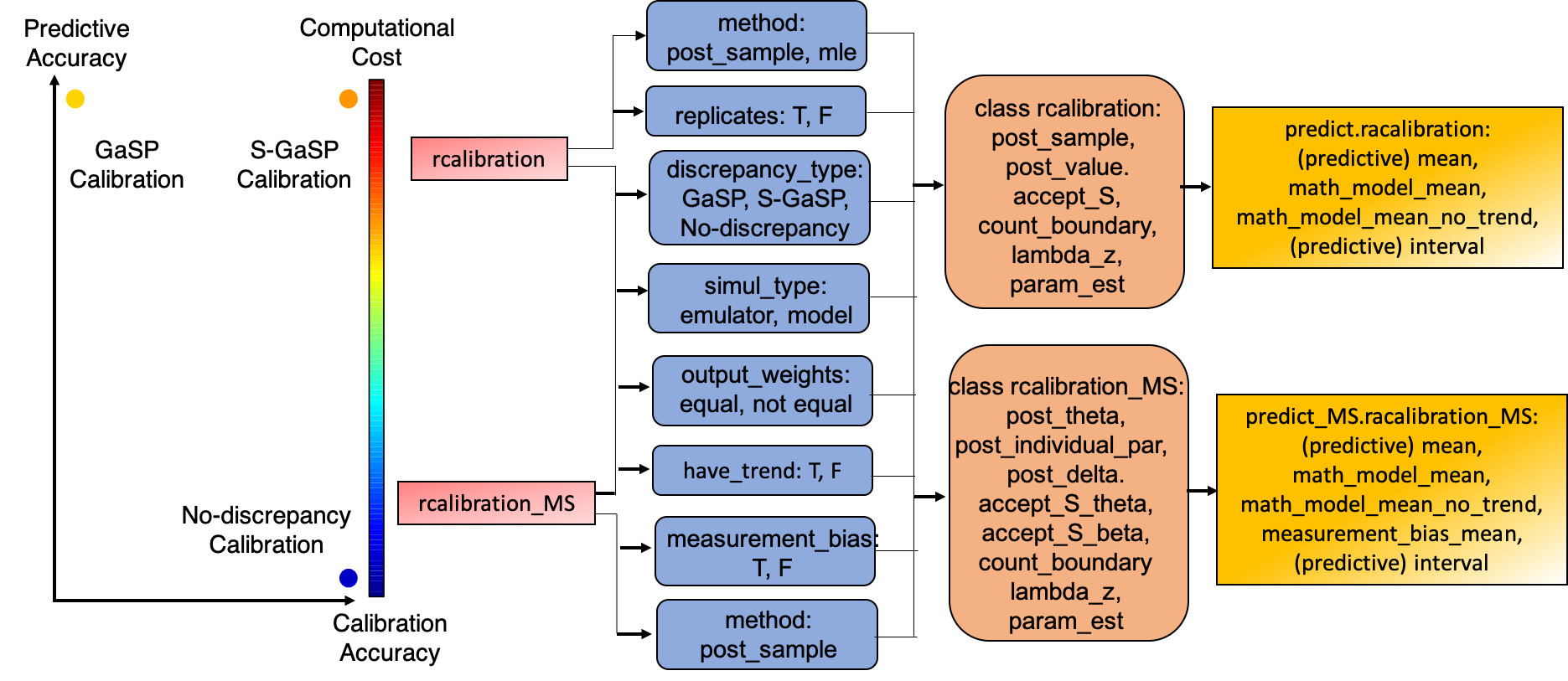
Figure 1: Schematic overview of the RobustCalibration package. The left panel show the predictive accuracy based on calibrated computer model and discrepancy versus calibration accuracy by calibrated computer model, evaluated by the $L_{2}$ loss to reality. The right panel give an overview of the major functions and classes in RobustCalibration. The calibration and calibration_MS in red boxes are the main function for parameter estimation for observations from single sources and from multiple sources, respectively. Some main arguments of these two functions are given in the blue boxes. The orange boxes give the object classes and main slots that will be created after calling calibration or calibration_MS functions. Finally, the object classes can be used for predicting the reality, either based on calibrated computer model and discrepancy, or by calibrated computer model alone.

Figure 1 gives a schematic overview of the RobustCalibration package. We consider two criteria by predicting the reality: using both calibrated computer model and discrepancy (predictive accuracy), and calibrated computer model alone (calibration accuracy), both evaluated in terms of the $L_{2}$ loss. The left panel gives comparison of accuracy and computational cost between the implemented methods. The no-discrepancy calibration is the fastest, as the main computational cost lies in approximating computer models by emulators or by numerical methods. The GaSP calibration and S-GaSP calibration have the same computational order, due to inverting the covariance matrix of the field data based on Cholesky decomposition. Because of the inclusion of the model of discrepancy, the predictive accuracy by GaSP and S-GaSP is the higher than the no-discrepancy calibration.

The RobustCalibration package can handle model calibration and prediction at a wide range of settings shown in blue boxes in Figure 1. First of all, both the posterior sampling and maximum likelihood estimator (MLE) were implemented in the rcalibration function. Users can choose no-discrepancy calibration and two different choices of modeling the discrepancy function (GaSP or S-GaSP) in modeling. Calibration models for replicates or repeated experiments (Bayarri et al., 2007b) based on sufficient statistics are also implemented, and the computational cost for repeated experiment is thus much smaller than direct implementation. For all scenarios, posterior sampling through the Markov chain Monte Carlo (MCMC) algorithm was implemented for Bayesian data inversion. Besides, we implement the MLE as a fast approach to obtain the point estimator of parameters for model calibration by a single source of data. After calling the rcalibration function, a "rcalibration" class (shown in the upper orange box) will be created , and prediction can be computed by calling the predict.calibration function (upper yellow box). Motivated by geophysical applications (Anderson et al., 2019), the rcalibration_MS function allows user to calibrate computer models using multiple sources of data or multiple types of observations, such as multiple images and time series. A “rcalibration_MS" class will be created by the rcalibration_MS function, and predict_MS.rcalibration_MS can be called for predictions.

Some computer models can be expensive to run, as the computer model outputs are typically numerical solutions of a system of differential equations. When computer model is slow, a statistical emulator is often used for approximating computationally expensive computer model. The GaSP emulator is a well-developed framework for emulating computationally expensive computer models and it was implemented in a few R packages, such as DiceKriging (Roustant et al., 2012), GPfit (MacDonald et al., 2015) and RobustGaSP (Gu et al., 2019). Here we use the functions rgasp, ppgasp and predict in RobustGaSP for emulating computer models with scalar-valued and vector-valued output, respectively.

Building packages for Bayesian model calibration is much more complicated than packages in statistical emulator, as both field observations and computer models are integrated. A few statistical packages are available for Bayesian model calibration, such as BACCO (Hankin, 2005), SAVE package (Palomo et al., 2015), and CaliCo (Carmassi et al., 2018). The CaliCo package, for example, integrates DiceKriging for emulating computational expensive simulations. It offers differen types of diagnostic plots based on ggplot2 (Wickham, 2011), and different prior choices of the parameters. The BACCO and SAVE consider the GaSP model of the discrepancy function (Kennedy and O’Hagan, 2001), and they emulate slow computer models by GaSP emulators as well.

Although a large number of studies were developed for Bayesian model calibration, to the authors’ best knowledge, many methods implemented in RobustCalibration were not implemented in another software package before. We highlight a few unique features of the RobustCalibration package. First of all, we allow users to specify different types of output of field observations, for different scenarios through the output argument in the rcalibration function. The simplest scenario is a vector output. We allow users to input a matrix type or a list for fields observations with the same or different number of replications, respectively. Efficient computation based on sufficient statistics was implemented for model calibration with replications, and it can improve the computation up to $k^{3}$ times, where $k$ is the number of repeated experiments. Second, models with different types and from multiple sources are can also be integrated for model calibration, based on the calibration_MS function. The measurement bias in each source can be modeled as correlated error by the argument measurement_bias=T in calibration_MS function. Third, we implemented emulators for approximating expensive computer models with both scalar-valued and vector-valued outputs. To the author’s knowledge, emulators for vector-valued outputs, especially at a large number of temporal or spatial coordinates, were not integrated in other packages for Bayesian model calibration. Here we use the parallel partial Gaussian stochastic process (PP-GaSP) emulator from RobustGaSP package (Gu et al., 2019) as a computationally scalable emulator of vector-valued output. The PP-GaSP model and RobustGaSP package (Gu et al., 2019) have been applied to various applications, such as emulating geophysical models of ground deformation (Anderson et al., 2019), storm surge simulation (Ma et al., 2019) and sea level observations (Ma et al., 2019). Furthermore, when computer models are imperfect, users can choose no-discrepancy, GaSP and S-GaSP models of discrepancy function. Finally, both posterior samples and MLE were implemented and made available by the method argument in the rcalibration function.

The rest of the paper is organized below. We first introduce the statistical framework for model calibration problem. Numerical examples and code will be provided along the methodology to illustrate the implemented methods in the RobustCalibration package. Then we give an overview of the architecture of the package, and we provide additional numerical examples for comparison. Closed form expressions of likelihood functions, derivatives, posterior distributions and computational algorithms are outlined in Appendix.

Statistical framework

We introduce the statistical framework in the this section, starting with the simplest method: no-discrepancy calibration. Then we discuss GaSP and S-GaSP models of discrepancy functions. For any kernel function, S-GaSP provides a transformed kernel from scaling the prior of the random $L_{2}$ loss between reality and computer models, often yielding a calibrated computer model close to the reality in terms of $L_{2}$ loss (Gu and Wang (2018)). We then introduce model calibration with repeated experiments, the statistical emulator for approximating computationally expensive computer models. Model calibration by data from multiple sources will be discussed at the end. Numerical examples and code from the RobustCalibration package will be provided along with the introduction.

No-discrepancy calibration

First, suppose we obtain a vector of real-valued field observations $\mathbf{y}^{F}=(y^{F}(\mathbf{x}_{1}),...,y^{F}(\mathbf{x}_{n}))^{T}$ at $n$ observable inputs. The corresponding computer model output is denoted by $\mathbf{f}^{M}_{\bm{\theta}}=(f^{M}(\mathbf{x}_{1},\bm{\theta}),...,f^{M}(\mathbf{x}_{n},\bm{\theta}))^{T}$ for any calibration parameters $\bm{\theta}$. Further assume the vector of measurement noise independently follows Gaussian distributions $\bm{\epsilon}\sim\mathcal{MN}(0,\,\sigma^{2}_{0}\bm{\Lambda})$, where the covariance of the noise is diagonal with the $i$th term being $\sigma^{2}_{0}\Lambda_{ii}$ and $\mathcal{MN}$ denote the multivariate Gaussian distribution. Here noises are independent and we will consider correlated noises based on multiple sources of data later. In the default setting, $\sigma^{2}_{0}$ is estimated by data and $\bm{\Lambda}=\mathbf{I}_{n}$, where $\mathbf{I}_{n}$ is an identity matrix with $n$ dimensions. Users can specify the inverse of the diagonal terms of $\bm{\Lambda}$ by the output_weights argument in rcalibration and rcalibration_MS functions, as variances of measurement errors can be different. We assume the diagonal matrix $\bm{\Lambda}$ is given in this section.

For a no-discrepancy calibration model in (1), the MLE of the variance of the noise is $\hat{\sigma}^{2}_{0}=S^{2}_{0}/n$ with $S^{2}_{0}=(\mathbf{y}^{F}-\mathbf{f}^{M}_{\theta})^{T}\bm{\Lambda}^{-1}(\mathbf{y}^{F}-\mathbf{f}^{M}_{\theta})$. The likelihood function is given in Appendix. As $\bm{\Lambda}$ is a diagonal matrix with diagonal terms denoted as $\Lambda_{ii}:=1/w_{i}$, the profile likelihood follows

$$\mathcal{L}(\bm{\theta}\mid\hat{\sigma}^{2}_{0})\propto\left\{\sum^{n}_{i=1}w_{i}\left(y^{F}(\mathbf{x}_{i})-f^{M}(\mathbf{x}_{i},\bm{\theta})\right)^{2}\right\}^{-n/2},$$

where $w_{i}=1$ is used in the default scenario. Note that maximizing the profile likelihood of a no-discrepancy model is equivalent to minimize $w_{i}\left(y^{F}(\mathbf{x}_{i})-f^{M}(\mathbf{x}_{i},\bm{\theta})\right)^{2}$, the weighted squared error loss on observed inputs. We numerical find $\bm{\theta}$ by the low-storage quasi-Newton optimization method (Nocedal, 1980; Liu and Nocedal, 1989) implemented in lbfgs function in the nloptr package (Ypma (2014)) for optimization.

In RobustCalibration package, we allow users to specify the trend or mean function modeled as $\bm{\mu}(\mathbf{x}_{i})=\mathbf{h}(\mathbf{x})\bm{\theta}_{m}=\sum^{q}_{t=1}h_{t}(\mathbf{x})\theta_{m,t}$ for any $\mathbf{x}$, where $\bm{\theta}_{m}=(\theta_{m,1},...,\theta_{m,q})^{T}$ is a vector of trend parameters. The MLE of the trend parameter is the least square estimator $\hat{\bm{\theta}}^{LS}_{m}=(\mathbf{H}^{T}\bm{\Lambda}^{-1}\mathbf{H})^{-1}\mathbf{H}^{T}\bm{\Lambda}^{-1}(\mathbf{y}^{F}-\mathbf{f}^{M}_{\theta})$ with $\mathbf{H}=(\mathbf{h}^{T}(\mathbf{x}_{1}),...,\mathbf{h}^{T}(\mathbf{x}_{n}))^{T}$ being an $n\times q$ matrix of the mean basis. It is easy to show maximizing the profile likelihood of a no-discrepancy model with a mean function is equivalent to minimize the squared error loss:

$$\bm{\hat{\theta}}_{LS}=\operatorname{argmin}_{\bm{\theta}}\sum^{n}_{i=1}w_{i}\left(y^{F}(\mathbf{x}_{i})-f^{M}(\mathbf{x}_{i},\bm{\theta})-\mathbf{h}(\mathbf{x}_{i})\hat{\bm{\theta}}^{LS}_{m}\right)^{2}.$$

After calling the rcalibration function with method=’mle’, the point estimator $\bm{\hat{\theta}}_{LS}$ is recorded in the slot param_est in the rcalibration class. The MLE is a computationally cheap way to obtain estimation of calibration parameter $\bm{\theta}$. After obtaining the MLE, we can use a plug the MLE into the computer model to compute the prediction of reality: $f^{M}(\mathbf{x}_{i},\bm{\hat{\theta}})+h(\mathbf{x}_{i})\hat{\bm{\theta}}^{LS}_{m}$. Computing the predictions, and predictive interval of the mean or observations were implemented in the predict function.

The uncertainty of the MLE can be hard to obtain, and the plug-in estimator does not propagate the uncertainty in prediction. To overcome this problem, we implement the MCMC algorithm for Bayesian inference. The posterior distributions follow

$$p(\bm{\theta}_{m},\sigma^{2}_{0},\bm{\theta}\mid\mathbf{y}^{F})\propto p(\mathbf{y}^{F}\mid\bm{\theta},{\bm{\theta}_{m}},\sigma^{2}_{0})\pi(\bm{\theta})\pi({\bm{\theta}_{m}},\sigma^{2}_{0}).$$ (3)

We assume an objective prior for the mean and variance parameters $\pi(\bm{\theta},\sigma^{2}_{0})\propto 1/\sigma^{2}_{0}$. The posterior distribution $p(\bm{\theta}_{m},\sigma^{2}_{0}\mid\bm{\theta},\mathbf{y}^{F})$ can be sampled from the Gibbs algorithm, since the prior is conjugate. Besides, we assume the default choice of the prior of the calibration parameters $\pi(\bm{\theta})$ to be uniform over the parameter space. The posterior distribution $p(\bm{\theta}\mid\mathbf{y}^{F},\bm{\theta}_{m},\sigma^{2}_{0})$ can be sampled from the Metropolis algorithm. The posterior distributions, MCMC algorithm and predictions from the posterior samples will be discussed in Appendix.

Here we show one example from Bayarri et al. (2007b), where data are observed from unknown reality: $y^{F}(x)=3.5\exp(-1.7x)+1.5+\epsilon$, where $\epsilon\sim\mathcal{N}(0,0.3^{2})$. We have 30 observations at 10 inputs in the domain $x_{i}\in[0,3]$, for $i=1,2,...,10$, each containing $3$ replications. The computer model is $f^{M}(x,\theta)=5\exp(-\theta x)$ with $\theta\in[0,\,50]$. The goal is to estimate the calibration parameters and predict the unknown reality ($3.5\exp(-1.7x)+1.5$) at $x\in[0,5]$.

We use the exact observable inputs and observations given in Bayarri et al. (2007b) generated by the code below.

R> input=c(.110, .432, .754, 1.077, 1.399, 1.721, 2.043, 2.366, 2.688,3.010)R> n=length(input)R> k=3R> output=t(matrix(c(4.730,4.720,4.234,3.177,2.966,3.653,1.970,2.267,2.084,2.079,+                2.409,2.371,  1.908,1.665,1.685, 1.773,1.603,1.922,1.370,1.661,+                1.757, 1.868,1.505,1.638,1.390, 1.275,1.679,1.461,1.157,1.530),k,n))R> Bayarri_07<-function(x,theta){+   5*exp(-x*theta)+ }R> theta_range=matrix(c(0,50),1,2)Here the mathematical model has a closed form expression so we input it as a function called Bayarri_07. The parameter range of calibration parameter $\theta$ is given by a vector called theta_range. Here the mathematical model has a closed-form expression. We will discuss calibrating computer models written as differential equations in the next example.

Calibrating a mathematical model by the no-discrepancy calibration can be implemented by the code below.

R> set.seed(1)R> X=matrix(1,n,1)R> m_no_discrepancy=rcalibration(input, output,math_model = Bayarri_07,+                                theta_range = theta_range, X =X,+                                have_trend = T,discrepancy_type = ’no-discrepancy’)R> m_no_discrepancytype of discrepancy function:  no-discrepancynumber of after burn-in posterior:  80000.1385 of proposed calibration parameters are acceptedmedian and 95\% posterior credible interval of calibration parameter  1 are2.951997 2.264356 3.930725Here we give a constant mean basis using the trend argument X, such that the mathematical model is $f^{M}(x,\theta)+\mu$. We draw $10,000$ posterior samples with the first $2,000$ as burn-in samples. One can adjust the number of posterior samples by argument S and S_0 in the calibration function. The median of the posterior samples of $\theta$ is $2.95$, and the $95\%$ posterior interval interval is around $(2.26,3.93)$. Around $14\%$ samples was accepted by the Metropolis algorithm. To use a proposal distribution of the calibration parameter with a smaller standard deviation, one can adjust sd_proposal below

R> m_no_discrepancy_small_sd=rcalibration(input, output,math_model = Bayarri_07,+                           theta_range = theta_range,+                           sd_proposal = c(rep(0.025,dim(theta_range)[1]),+                                            rep(0.25,dim(as.matrix(input) )[2]),0.25),+                           X =X, have_trend = T,discrepancy_type = ’no-discrepancy’)R> m_no_discrepancy_small_sdtype of discrepancy function:  no-discrepancynumber of after burn-in posterior:  80000.2613 of proposed calibration parameters are acceptedmedian and 95\% posterior credible interval of calibration parameter  1 are2.935007 2.19352 3.933492Here the first $p_{\theta}$ terms in sd_proposal is the standard deviation of the proposal distribution of the calibration parameter, chosen as $0.025$ of the range of the calibration parameter. The default choice is $0.05$. The next $p_{x}+1$ parameters are standard deviation of the inverse logarithm of the range parameter and nugget parameters in GaSP and S-GaSP calibration, discussed in following subsections. The median and $95\%$ posterior credible interval with different proposal distributions do not change much in the no-discrepancy calibration in this example.

The following code gives predictions of the reality using the calibrated computer model and estimated mean with a constant mean basis by argument X_testing. We make predictions on 200 test inputs equally spaced at $x\in[0,5]$. We also compute the $95\%$ predictive interval by argument interval_est.

R> testing_input=seq(0,5,5/199)R> X_testing=matrix(1,length(testing_input),1)R> m_no_discrepancy_pred=predict(m_no_discrepancy,testing_input,math_model=Bayarri_07,+                               interval_est=c(0.025, 0.975),X_testing=X_testing)

Posterior samples of the calibration parameter $\theta$ and the mean parameter $\theta_{m}$ in the no-discrepancy calibration are graphed as the red rectangles in the right panel in Figure 2. The predictive mean and 95% predictive interval are graphed as the red curve and grade shaded area in the left panel, respectively. Compared to models with an estimated discrepancy function, the posterior samples from the no-discrepancy calibration are more concentrated, and the average length of 95% predictive interval is shorter. However, a large proportion of reality at $x\in[0,1.5]$ is not covered by the 95% posterior credible interval, due to large discrepancy between the mathematical model and reality in this domain. Next we introduce two models of discrepancy to solve this problem.

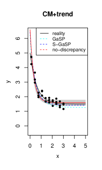
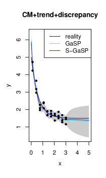
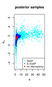
Figure 2: Predictions and posterior samples by the RobustCalibvration package for the example introduced in Bayarri et al. (2007b). In the left and middle panels, The unknown reality is graphed as black curves, and field observations that contain with 3 replicates at each observable input are plotted as black circles. In the left panel, predictions of reality based on calibrated computer model (including the estimated trend parameter) by GaSP, S-GaSP and no-discrepancy calibration are graphed as light blue, blue and red curves, respectively. ‘CM’ in the tile denotes the computer model and the shaded area is the $95\%$ posterior predictive interval by the no-discrepancy calibration. In the middle panel, predictions based on the calibrated computer model, discrepancy and trend by GaSP and S-GaSP are graphed as lightblue and blue curves, respectively. The shaded area is the $95\%$ posterior predictive interval by the GaSP calibration. After burn-in posterior samples of calibration parameter $\theta$ and mean parameter $\theta_{m}$ by these three models are plotted in the right panel.

Gaussian stochastic process model of discrepancy function

Assume the discrepancy function is modeled as a GaSP, meaning that for any $\{\mathbf{x}_{1},...,\mathbf{x}_{n}\}$, the marginal distribution of discrepancy function follows a multivariate normal distribution:

$$(\delta(\mathbf{x}_{1}),...,\delta(\mathbf{x}_{n}))^{T}\mid\bm{\mu},\sigma^{2},\mathbf{R}\sim\mathcal{MN}(\bm{\mu},\,\sigma^{2}\mathbf{R}),$$

where $\bm{\mu}=(\mu(\mathbf{x}_{1}),...,\mu(\mathbf{x}_{n}))^{T}$ is a vector of the mean (or trend), $\sigma^{2}$ is a variance parameter, and $\mathbf{R}$ is the correlation matrix between outputs.

Similar to the no-discrepancy calibration, we allow user to model the trend as $\bm{\mu}(\mathbf{x}_{i})=h(\mathbf{x}_{i})\bm{\theta}_{m}=\sum^{q}_{t=1}h_{t}(\mathbf{x}_{i})\theta_{m,t}$, where $h(\mathbf{x}_{i})$ is a row vector of mean basis and $\bm{\theta}_{m}$ is a vector of trend parameters. Since the trend is often modeled in the computer model, the default value of the trend parameters is $\mathbf{0}$.

The $(i,j)$th element of the correlation matrix is modeled by a kernel function $R_{i,j}=K(\mathbf{x}_{i},\mathbf{x}_{j})$. We implement the separable kernel $K(\mathbf{x}_{i},\mathbf{x}_{j})=\prod^{p_{x}}_{l=1}K_{l}(\mathbf{x}_{i},\mathbf{x}_{j})$, where $K_{l}$ models the correlation between the $l$th coordinate of the observable input, for $l=1,...,p_{x}$. Some frequently used kernel functions are listed in Table 1. The range parameters $\bm{\gamma}$ are estimated by default.

GaSP calibration	Product kernel ($K(\mathbf{d})=\prod^{p_{x}}_{l=1}K_{l}(d_{l})$)
Matérn $\alpha=5/2$	$K_{l}(d_{l})=\left(1+\frac{\sqrt{5}d_{l}}{\gamma_{l}}+\frac{5d^{2}_{l}}{3\gamma_{l}^{2}}\right)\exp\left(-\frac{\sqrt{5}d_{l}}{\gamma_{l}}\right)$
Matérn $\alpha=3/2$	$K_{l}(d_{l})=\left(1+\frac{\sqrt{3}d_{l}}{\gamma_{l}}\right)\exp\left(-\frac{\sqrt{3}d_{l}}{\gamma_{l}}\right)$
Power exponential	$K_{l}(d_{l})=\exp\left\{-\left(\frac{d_{l}}{\gamma_{l}}\right)^{\alpha_{l}}\right\}$, $0<\alpha_{l}\leq 2$
S-GaSP calibration	Scaled kernel ($K_{Z_{d}}(\mathbf{x}_{a},\mathbf{x}_{b})=K(\mathbf{x}_{a},\mathbf{x}_{b})-\mathbf{r}^{T}(\mathbf{x}_{a}){\mathbf{R}}_{z}^{-1}\mathbf{r}(\mathbf{x}_{b})$)

Table 1: Correlation functions currently implemented in RobustCalibration. For any $\mathbf{x}_{a},\mathbf{x}_{b}\in\mathcal{X}$, denote $\mathbf{d}=\mathbf{x}_{a}-\mathbf{x}_{d}=(d_{1},...,d_{p_{x}})^{T}$. For any kernel $K$, the discretized scaled kernel $K_{Z_{d}}(\mathbf{x}_{a},\mathbf{x}_{b})$ with discretization points on observed points $\mathbf{x}_{1},...,\mathbf{x}_{n}$ was implemented in the S-GaSP calibration, where ${\mathbf{R}}_{z}:=\mathbf{R}+n\mathbf{I}_{n}/\lambda_{z}$, and $\mathbf{r}(\mathbf{x})=(K(\mathbf{x},\mathbf{x}_{1}),...,K(\mathbf{x},\mathbf{x}_{n}))^{T}$ for any $\mathbf{x}$.

Denote the nugget parameter by the noise variance to signal variance ratio $\eta=\sigma^{2}_{0}/\sigma^{2}$. Marginalizing out discrepancy $\delta$, one has $\mathbf{y}^{F}\sim\mathcal{MN}(\mathbf{f}^{M}_{\theta}+\mathbf{H}\bm{\theta}_{m},\,\sigma^{2}_{0}\tilde{\mathbf{R}})$, where $\tilde{\mathbf{R}}=\mathbf{R}/\eta+\bm{\Lambda}$. Here by default $\bm{\Lambda}=\mathbf{I}_{n}$, and we allow users to specify the inverse diagonal terms of $\bm{\Lambda}$ by the argument weights: $w_{i}=1/\Lambda_{ii}$, for $i=1,...,n$.

The MLE of the trend and noise variance parameters in the GaSP calibration follows $\hat{\bm{\theta}}_{m}=\left(\mathbf{H}^{T}{{\mathbf{\tilde{R}}}}^{-1}\mathbf{H}\right)^{-1}\mathbf{H}^{T}{{\mathbf{\tilde{R}}}}^{-1}{(\mathbf{y}-\mathbf{f}^{M}_{\theta})}$ and $\hat{\sigma}^{2}_{0}=S^{2}_{K}/n$, where $S^{2}_{K}=(\mathbf{y}-\mathbf{f}^{M}_{\theta}-\mathbf{H}^{T}\hat{\bm{\theta}}_{m})^{T}{{\mathbf{\tilde{R}}}}^{-1}(\mathbf{y}-\mathbf{f}^{M}_{\theta}-\mathbf{H}^{T}\hat{\bm{\theta}}_{m})$. Plugging the MLE of trend and noise variance parameters, one can numerically maximize the profile likelihood to obtain the calibration, kernel and nugget parameters in GaSP calibration:

$$(\hat{\bm{\theta}},\hat{\bm{\gamma}},\hat{\eta})=\operatorname*{argmax}_{(\bm{\theta},\bm{\gamma},\eta)}\mathcal{L}_{K}(\bm{\theta},\bm{\gamma},\eta,\mid\hat{\bm{\theta}}_{m},\hat{\sigma}^{2}_{0})$$ (4)

where the profile likelihood $\mathcal{L}_{K}(\bm{\theta},\bm{\gamma},\eta,\mid{\hat{\bm{\theta}}_{m}},\hat{\sigma}^{2}_{0})$ with kernel $K(.,.)$ has a closed form expression, given in the Appendix.

After obtaining the estimation of the parameters, the predictive distribution of reality on any $\mathbf{x}^{*}$ can be obtained by plugging the estimator

$$y^{R}(\mathbf{x}^{*})\mid\mathbf{y}^{F},\hat{\bm{\theta}}_{m},\hat{\sigma}^{2}_{0},\hat{\bm{\theta}},\hat{\bm{\gamma}},\hat{\eta}\sim\mathcal{N}(\hat{\mu}(\mathbf{x}^{*}),\hat{\sigma}^{2}_{0}(K^{*}/\hat{\eta}+\Lambda^{*})),$$ (5)

where $\Lambda^{*}$ is the weight at $\mathbf{x}^{*}$ set to be 1 by default, and

$$\hat{\mu}(\mathbf{x}^{*}) =f^{M}(\mathbf{x}^{*},\hat{\bm{\theta}})+\mathbf{h}(\mathbf{x}^{*})\hat{\bm{\theta}}_{m}+\mathbf{r}^{T}(\mathbf{x}^{*})\tilde{\mathbf{R}}^{-1}(\mathbf{y}^{F}-\mathbf{f}(\mathbf{x}_{1:n},\hat{\bm{\theta}})-\mathbf{H}\hat{\bm{\theta}}_{m}),$$

$$K^{*} =K(\mathbf{x}^{*},\mathbf{x}^{*})-\mathbf{r}^{T}(\mathbf{x}^{*})\tilde{\mathbf{R}}^{-1}\mathbf{r}(\mathbf{x}^{*}),$$

with $\mathbf{r}(\mathbf{x}^{*})=(K(\mathbf{x}^{*},\mathbf{x}_{1}),...,K(\mathbf{x}^{*},\mathbf{x}_{n}))^{T}$. Noting that the calibrated computer model $f^{M}(\mathbf{x}^{*},\hat{\bm{\theta}})$ is of interest for predicting the reality, due to its interpretability. Thus, we recorded three slots for predicting the reality: 1) math_model_mean_no_trend ($f^{M}(\mathbf{x}^{*},\hat{\bm{\theta}})$), 2) math_model_mean ($f^{M}(\mathbf{x}^{*},\hat{\bm{\theta}})+\mathbf{h}(\mathbf{x}^{*})\hat{\bm{\theta}}_{m}$), and 3) mean ($\hat{\mu}(\mathbf{x}^{*})$). Furthermore, users can also output the predictive interval from the predictive distribution in (5) by letting argument interval_est=T and specifying interval_est in the predict.rcalibration function. For example, setting interval_est=c(0.025,0.975) in the predict.rcalibration function gives the 95% predictive interval of the reality. Furthermore, if interval_data=T, the predictive interval of the data will be computed.

Numerically computing MLE can be unstable as the profile likelihood $\mathcal{L}_{K}(\bm{\theta},\bm{\gamma},\eta\mid{\bm{\hat{}}\theta_{m}},\hat{\sigma}^{2}_{0})$ is nonlinear and nonconvex with respect to the parameters $(\bm{\theta},\bm{\gamma},\eta)$. To obtain the uncertainty assessment of parameter estimation and to avoid instability in numerical search of MLE, we implement the MCMC algorithm for Bayesian inference. The posterior distribution is

$$p(\bm{\theta}_{m},\sigma^{2}_{0},\bm{\theta},\bm{\gamma},\eta\mid\mathbf{y}^{F})\propto p_{K}(\mathbf{y}^{F}\mid\bm{\theta},\bm{\gamma},\eta,{\bm{\theta}_{m}},\sigma^{2}_{0})\pi(\bm{\theta})\pi({\bm{\theta}_{m}},\sigma^{2}_{0},\bm{\gamma},\eta),$$ (6)

where $p_{K}(.)$ is the multivariate normal density with covariance function of the discrepancy being $\sigma^{2}K(\cdot,\cdot)$, and $\pi(\bm{\theta})$ is the prior of the calibration parameters, assumed to be uniform over the parameter space. The prior of the mean, variance, kernel and nugget parameters takes the form below

$$\pi({\bm{\theta}_{m}},\sigma^{2}_{0},\bm{\gamma},\eta)\propto\frac{\pi(\bm{\gamma},\eta)}{\sigma^{2}_{0}},$$

where the usual reference prior of the trend and variance parameters $\pi({\bm{\theta}_{m}},\sigma^{2}_{0})\propto 1/\sigma^{2}_{0}$ is assumed. We use jointly robust prior for the kernel and nugget parameters $\pi(\bm{\gamma},\eta)$, as it has a similar tail density decay rate as the reference prior, but it is easier and more robust to compute (Gu, 2019). Closed form expressions of the posterior distributions and MCMC algorithm are provided in Appendix.

In RobustCalibration, we record the posterior samples after burn-in $(\bm{\theta}^{(i)}_{m},(\sigma^{2}_{0})^{(i)},\bm{\theta}^{(i)},\bm{\gamma}^{(i)},\eta^{(i)})$ for $i=S_{0}+1,...,S$. Users can also record a subset of posterior samples for storage reasons by thinning the Markov chain. For instance, if $1/5$ of the posterior samples shall be recorded, users can set thinning=5 in the rcalibration function.

Similar to the predictions based on MLE, we also output three types of predictions. For instance, suppose we obtain $S$ posterior samples with first $S_{0}$ samples used as burn-in samples, the predictive mean of the reality can be computed by

$$\hat{\mu}(\mathbf{x}^{*})=\sum^{S}_{i=S_{0}+1}f^{M}(\mathbf{x}^{*},{\bm{\theta}}^{(i)})+\mathbf{h}(\mathbf{x}^{*}){\bm{\theta}_{m}^{(i)}}+(\mathbf{r}^{(i)}(\mathbf{x}^{*}))^{T}(\tilde{\mathbf{R}}^{(i)})^{-1}(\mathbf{y}^{F}-\mathbf{f}^{M}(\mathbf{x}_{1:n},{\bm{\theta}}^{(i)})-\mathbf{H}{\bm{\theta}_{m}^{(i)}})$$

where $\mathbf{r}^{(i)}(\mathbf{x}^{*})$ and ${\mathbf{\tilde{R}}}^{(i)}$ are obtained by plugging in the $i$th posterior samples. The predictive interval can also be computed by specifying the argument interval_est in predict.rcalibration function.

Code below implements the GaSP calibration of parameter estimation and predictions for the example in (Bayarri et al., 2007b) that was discussed in the previous subsection.

R> m_gasp=rcalibration(input, output,math_model = Bayarri_07,theta_range = theta_range,+                     X =X, have_trend = T,discrepancy_type = ’GaSP’)R> m_gasp_pred=predict(m_gasp,testing_input,math_model=Bayarri_07,+                     interval_est=c(0.025, 0.975),X_testing=X_testing)

Predictions and posterior samples from the GaSP calibration are graphed in Figure 2. The associated predictive error is shown in Table 2. Comparing the first two rows in Table 2, the predictive RMSE in the no-discrepancy calibration is around $0.25$, and it decreases to $0.15$, after adding the discrepancy function modeled by GaSP. Around 97.5% of the held-out truth is covered by the 95% credible interval of the reality in GaSP calibration, indicating accurate uncertainty assessment of the prediction in this example. In comparison, the 95% credible interval of the reality in no-discrepancy calibration only covers around $80\%$ of the held-out reality.

As shown in the right panel in Figure 2, the posterior samples from GaSP spread over a larger parameter range, reflecting larger uncertainty in the parameter space. This is because the discrepancy modeled by GaSP with the frequently used kernel listed in Table 1 is very flexible. As a result, the calibrated mathematical model alone may be less accurate in predictive the reality. We discuss a recent approach that induces a scaled kernel to constrain the discrepancy function in the next subsection.

	RMSE (CM+trend)	RMSE (with discrepancy)	$P_{CI}(95\%)$	$L_{CI}(95\%)$
GaSP	0.253	0.151	0.975	0.880
S-GaSP	0.228	0.131	0.955	1.15
No-discrepancy	0.250	/	0.795	0.409

Table 2: Predictive accuracy and uncertainty assessment. The RMSE of the out-of-sample prediction based on the calibrated computer model (CM) and trend are shown in the second column. The predictive RMSE by the summation of the calibrated computer model, trend and discrepancy is given in the third column. The proportion of the held-out reality covered in the $95\%$ predictive interval, and average lengths of predictive intervals are given in the last two columns, respectively.

Calibration by scaled Gaussian stochastic process model of discrepancy

Scaling the kernel of GaSP for model calibration was introduced in Gu and Wang (2018), where the random $L_{2}$ distance between the discrepancy model was scaled to have more prior probability mass at small values, as small distance indicates the computer model fits the reality well. Note that we leave $\sigma^{2}$ as a free parameter estimated by data, and thus S-GaSP is a flexible model of discrepancy.

In RobustCalibration, we implemented the discretized S-GaSP to scale the random mean squared error between the reality and computer model:

$$\delta_{z_{d}}(\mathbf{x})=\left\{\delta(\mathbf{x})\mid\frac{1}{n}{\sum^{n}_{i=1}\delta(\mathbf{x}_{i})^{2}}=Z_{d}\right\},$$ (7)

with the subscript ‘d’ denoting discretization, and the density of $Z_{d}$ is defined as

$$p_{Z_{d}}(z) =\frac{g_{Z_{d}}\left(z\right)p_{\delta}\left(Z_{d}=z\right)}{\int_{0}^{\infty}g_{Z_{d}}\left(t\right)p_{\delta}\left(Z_{d}=t\right)dt},$$ (8)

where $p_{\delta}(Z_{d}=z)$ is the density of $Z_{d}$ induced by GaSP with kernel $K(\cdot,\cdot)$, and $g_{Z}(\cdot)$ is a nondecreasing function that places more probability mass on smaller values of the $L_{2}$ loss. For a frequently used kernel function in Table 1, the probability measure $p_{\delta}\left(Z_{d}=z\right)$ places a large probability at large $L_{2}$ loss when correlation is large, dragging the calibrated computer model away from the reality. In S-GaSP calibration, the measure for $Z_{d}$ was scaled to have more probability mass near zero by a scaling function $g_{Z_{d}}(z)$. The default scaling function is assumed to be an exponential distribution,

$$g_{Z_{d}}(z)=\frac{\lambda_{z}}{2\sigma^{2}}\exp\left(-\frac{\lambda_{z}z}{2\sigma^{2}}\right),$$ (9)

where $\lambda_{z}$ controls how large the scaling factor is. Large $\lambda_{z}$ induces more prior probability mass concentrating at the origin. As shown in Gu et al. (2022b), $\lambda_{z}\propto\sqrt{n}$ guarantees the convergence of the calibration parameters to the ones that minimize the $L_{2}$ distance between the reality and computer model. Furthermore, the calibrated computer models can be far away from reality when the nugget $\eta$ is small and the range $\bm{\gamma}$ is large (corresponding to a large correlation). Thus we let the default choice be $\lambda_{z}=(\lambda||\bm{\tilde{\gamma}}||)^{-1/2}$, where $\lambda=(\sigma^{2}_{0}/\sigma^{2}n)$ being the regularization parameter in the kernel ridge regression, and $\tilde{\bm{\gamma}}=(\gamma_{1}/L_{1},...,\gamma_{p_{x}}/L_{p_{x}})^{T}$, with $L_{i}$ being the length of domain of the $i$th coordinate of the calibration parameter . We allow users to specify the scaling parameters by the lambda_z in the rcalibration function.

The default choice of kernel scaling in (8) and (9) has computational advantages. After marginalizing out $Z_{d}$, it follows from Lemma 2.4 in Gu and Wang (2018) that $\delta_{z_{d}}(\cdot)$ has the covariance function

$$\sigma^{2}K_{z_{d}}(\mathbf{x}_{a},\mathbf{x}_{b})=\sigma^{2}\left\{K(\mathbf{x}_{a},\mathbf{x}_{b})-\mathbf{r}^{T}(\mathbf{x}_{a})\left(\mathbf{R}+\frac{n\mathbf{I}_{n}}{\lambda_{z}}\right)^{-1}\mathbf{r}(\mathbf{x}_{b})\right\},$$ (10)

for any $\mathbf{x}_{a},\mathbf{x}_{b}$, where $\mathbf{r}(\mathbf{x})=(K(\mathbf{x},\mathbf{x}_{1}),...,K(\mathbf{x},\mathbf{x}_{n}))^{T}$ for any $\mathbf{x}$. The covariance matrix of the S-GaSP model of $(\delta_{z}(\mathbf{x}_{1}),...,\delta_{z}(\mathbf{x}_{n}))^{T}$ follows

$$\sigma^{2}\mathbf{R}_{z}=\sigma^{2}\left\{\mathbf{R}-\mathbf{R}\left(\mathbf{R}+\frac{n\mathbf{I}_{n}}{\lambda_{z}}\right)^{-1}\mathbf{R}\right\}.$$ (11)

The closed-form expression in Equ. (10) avoids sampling $(\delta_{z}(\mathbf{x}_{1}),...,\delta_{z}(\mathbf{x}_{n}))$ to obtain $Z_{d}$ from the posterior distribution, which greatly improves the computational speed.

For any covariance function $K(\cdot,\cdot)$ in GaSP calibration, a scaled kernel was induced in S-GaSP calibration, shown in the last row of Table 1. The S-GaSP model of the discrepancy can be specified by the argument discrepancy_type=’S-GaSP’ in the rcalibration function. Similar to the model of GaSP-calibration, we also provide MLE and posterior samples for estimating the parameters, with argument method=’mle’ and method=’post_sample’, respectively. The MLE of parameters in S-GaSP are computed by maximizing the profile likelihood

$$(\hat{\bm{\theta}},\hat{\bm{\gamma}},\hat{\eta})=\operatorname*{argmax}_{(\bm{\theta},\bm{\gamma},\eta)}\mathcal{L}_{K_{Z_{d}}}(\bm{\theta},\bm{\gamma},\eta,\mid{\hat{\bm{\theta}}_{m}},\hat{\sigma}^{2}_{0})$$ (12)

where $({\hat{\bm{\theta}}_{m}},\hat{\sigma}^{2}_{0})$ denotes the MLE of trend and noise variance parameters in S-GaSP calibration, and $\mathcal{L}_{K_{Z_{d}}}$ is the profile likelihood with respect to scaled kernel $K_{Z_{d}}$ in (10) of modeling the discrepancy. Here one can simply replace the kernel $K$ from GaSP calibration to kernel $K_{Z_{d}}$ from S-GaSP calibration. Furthermore, predictions and intervals can be obtained by predict.rcalibration function as well.

We provide the code that implements S-GaSP calibration and prediction of the example in Bayarri et al. (2007b) below.

R> m_sgasp=rcalibration(input, output,math_model = Bayarri_07,theta_range = theta_range,+                      X =X, have_trend = T,discrepancy_type = ’S-GaSP’)R> m_sgasp_pred=predict(m_sgasp,testing_input,math_model=Bayarri_07,+                      interval_est=c(0.025, 0.975),X_testing=X_testing)

Predictions from S-GaSP are graphed as blue curves in Figure 2 and numerical comparisons are given in Table 2. With an estimated discrepancy by S-GaSP, the prediction of reality is more accurate at $x\in[0.5,1.5]$, compared to no-discrepancy calibration. Note that the prediction by the S-GaSP model also extrapolates the reality at $x\in[3,5]$ accurately, because the calibrated computer model is closer to the truth. Furthermore, the 95% posterior credible interval by S-GaSP covers around $95\%$ of the held-out samples.

Calibration with repeated experiments

Repeated experiments or replicates are commonly used in experiments to validate a scientific finding, or to reproduce experimental outcomes. Obtaining a set of replicates of the same experiment is helpful to reduce the experimental error. Consider, for example, $k_{i}$ replicates are available for each observable input $\mathbf{x}_{i}$, denoted as $\mathbf{y}^{F}_{i}=(y_{1}^{F}(\mathbf{x}_{i}),...,y^{F}_{k_{i}}(\mathbf{x}_{i}))^{T}$. Denote $\bar{\mathbf{y}}^{F}=(\sum^{k_{1}}_{j=1}y^{F}_{j}(\mathbf{x}_{1})/k_{1},...,\sum^{k_{n}}_{j=1}y^{F}_{j}(\mathbf{x}_{n})/k_{n})^{T}$ the aggregated data. The probability density of the field observations can be written as

$$p(\mathbf{y}^{F}_{1},...,\mathbf{y}^{F}_{n}\mid\bm{\mu},\bm{\delta},\bm{\theta},\sigma^{2}_{0}) =(2\pi\sigma^{2}_{0})^{-\frac{\sum^{n}_{i=1}k_{i}}{2}}\exp\left(-\frac{\sum^{n}_{i=1}\omega_{i}\sum^{k_{i}}_{j=1}(y^{F}_{j}(\mathbf{x}_{i})-f^{M}(\mathbf{x}_{i},\bm{\theta})-\mu_{i}-\delta(\mathbf{x}_{i}))^{2}}{2\sigma^{2}_{0}}\right)$$

$$=(2\pi\sigma^{2}_{0})^{-\frac{\sum^{n}_{i=1}k_{i}}{2}}\exp\left(-\frac{S^{2}_{f}}{2\sigma^{2}_{0}}-\frac{\sum^{n}_{i=1}k_{i}\omega_{i}(\bar{y}^{F}_{i}-f^{M}(\mathbf{x}_{i},\bm{\theta})-\mu_{i}-\delta(\mathbf{x}_{i}))^{2}}{2\sigma^{2}_{0}}\right)$$

where $S^{2}_{f}=\sum^{n}_{i=1}\omega_{i}\sum^{k_{i}}_{j=1}(y^{F}_{j}(\mathbf{x}_{i})-\bar{y}^{F}_{i})^{2}=\sum^{n}_{i=1}{\omega_{i}(\mathbf{y}^{F}_{i}-\bar{y}^{F}_{i}\mathbf{1}_{k_{i}})^{T}(\mathbf{y}^{F}_{i}-\bar{y}^{F}_{i}\mathbf{1}_{k_{i}})}$ with subscript ‘f’ denoting field observations. After integrating out the discrepancy term, assumed to be modeled as a GaSP, the marginal likelihood of the parameters follows

$$\mathcal{L}_{K}(\bm{\theta},\bm{\theta}_{m},\sigma^{2}_{0},\bm{\gamma},\eta)\propto(\sigma^{2}_{0})^{-\frac{\sum^{n}_{i=1}k_{i}}{2}}|\tilde{\tilde{\bm{R}}}|^{-\frac{1}{2}}\exp\left\{-\frac{(\bar{\mathbf{y}}^{F}-\mathbf{f}^{M}_{\theta}-\mu\mathbf{1}_{n})^{T}\tilde{\tilde{\bm{R}}}^{-1}(\bar{\mathbf{y}}^{F}-\mathbf{f}^{M}_{\theta}-\mu\mathbf{1}_{n})}{2\sigma^{2}_{0}}-\frac{S^{2}_{f}}{2\sigma^{2}_{0}}\right\},$$ (13)

where $\tilde{\tilde{\bm{R}}}=(\mathbf{R}/\eta+\tilde{\bm{\Lambda}})$, with $\tilde{\bm{\Lambda}}$ being an diagonal matrix with diagonal entry $\Lambda_{ii}=1/(\omega_{i}k_{i})$, for $i=1,2,...,n$, and $\eta=\sigma^{2}_{0}/\sigma^{2}$. The S-GaSP calibration with replications can also be defined, by simply replacing $\mathbf{R}$ by $\mathbf{R}_{z}$ where the $(i,j)$th term is defined by the scaled kernel in Table 1.

The likelihood in (13) has a clear computational advantage. If one directly computes the covariance and its inversion, the computational complexity is $O((\sum^{n}_{i=1}k_{i})^{3})$, while the computational order by Equation (13) is only $O(n^{3})+O(\sum^{n}_{i=1}k_{i})$. Suppose $k_{i}=k$, for $i=1,...,n$, using Equation (13) is around $k^{3}$ times faster than directly computing the likelihood, with no loss of information.

In RobustCalibration package, one can specify replications by inputting a $n\times k$ matrix into the argument observations in the rcalibration function for scenarios with $n$ observable inputs, each containing $k$ repeated measurements. Or one can give a list observations in the rcalibration function with size $n$, where each element in the list contains $k_{i}$ values of replicates, for $i=1,...,n$. For observations with replicates, MLE and posterior sampling were implemented in rcalibration function, and predictions were implemented in predict.rcalibration function.

Statistical emulator

In RobustCalibration package, users can specify a mathematical model by math_model in rcalibration function, if the closed form expression of the mathematical model is available. However, closed form solutions of physical systems are typically unavailable and numerical solvers are required. Simulating the outputs from computer models can be slow. For instance, the TITAN2D computer model of simulating pyroclastic flows for geological hazard quantification takes roughly 8 minutes per set of inputs (Simakov et al., 2019). As hundreds of thousands of model runs are sometimes required for model calibration, directly computing the computer model by numerical methods is often prohibitive. In this scenario, we construct a statistical emulator as a surrogate model, to approximate the computer simulation, based on a small number of computer model runs. Gaussian stochastic process emulator has been widely used as a surrogate model for emulating computer experiments (Sacks et al., 1989).

To start with, assume we obtained the output of computer model at $D$ input design points, $(\bm{\theta}_{1},...,\bm{\theta}_{D})$, often selected from an “in-fill" design, such as the latin hypercube design (Santner et al., 2003). There are two types of computer model outputs: 1) scalar-valued output: $f^{M}(\bm{\theta})\in\mathbb{R}$, and 2) vectorized output at $k$ coordinates $\mathbf{f}^{M}(\mathbf{x}_{1:k},\bm{\theta})\in\mathbb{R}^{k}$, where $k$ can be as large as $10^{6}$. Various packages are available for fitting scalar-valued GP emulators, such as DiceKriging (Roustant et al. (2012)), GPfit (MacDonald et al. (2015)), and RobustGaSP (Gu et al. (2019)). Some of these packages were used in Bayesian model calibration packages (Palomo et al., 2015; Carmassi et al., 2018). However, the emulator of the vectorized output was rarely integrated for model calibration.

In Robustcalibration, we call the rgasp function and ppgasp function from the RobustGaSP package for emulating scalar-valued and vectorized computer model outputs, respectively. The parallel partial Gaussian process (PP-GaSP) by the ppgasp function has two advantages. First, computing the predictive mean by the PP-GaSP only takes $O(kD)+O(D^{3})$ operations. The linear computational order with respect to $k$ is suitable for computer model at a massive size of coordinates. Second, the PP-GaSP emulator is typically more robust compared to other methods, as covariance over $\bm{\theta}$ is shared across all grids. Further more, the kernel parameters are estimated by the marginal posterior mode with robust parameterization, typically avoiding the degenerated scenarios that causes poor emulation results (Gu (2019)).

To call the emulator, users can select argument simulator=0, and then input the simulation runs into arguments input_simul, and output_simul. One can input a vector into output_simul to emulate scalar-valued computer models, or a matrix into output_simul to call the PP-GaSP emulator for vectorized outputs. For both scenarios, we use a modular approach of fitting PP-GaSP emulator advocated in e.g. (Bayarri et al., 2007b; Liu et al., 2009), where the predictive distribution of the emulator depends on simulator runs, but not field observations. After fitting an emulator, the predictive mean of the PP-GaSP emulator will be used to approximate the computer model at any unobserved $\bm{\theta}^{*}$ by default.

We illustrate the efficiency and accuracy of the PP-GaSP emulator for approximating ordinary different equations (ODEs) from Box and Coutie (1956), where the interaction between two chemical substances $y_{1}$ and $y_{2}$ are modeled as

$$\dot{y}_{1}(t) =10^{\theta_{1}-3}y_{1}(t),$$

$$\dot{y}_{2}(t) =10^{\theta_{1}-3}y_{1}(t)-10^{\theta_{2}-3}{y}_{2}(t).$$

In each of the 6 time point $t=10,20,40,80,160$ and $320$, 2 replicates of the second chemical substance are available in Box and Coutie (1956). Initial conditions are $y_{1}(t=0)=100$ and $y_{2}(t=0)=0$. The computer model contains two parameters $\theta_{1}\in[0.5,1.5]$ and $\theta_{2}\in[0.5,1.5]$.

To start with, we first define the ODEs and implement the default method in the ode function from the deSolve package (Soetaert et al., 2010), to numerically solve the ODEs at a given initial condition and parameter set.

library(deSolve)R> Box_model <- function(time, state, parameters) {+   par <- as.list(c(state, parameters))+   with(par, {+     dM1=-10^{parameters[1]-3}*M1+     dM2=10^{parameters[1]-3}*M1-10^{parameters[2]-3}*M2+     list(c(dM1, dM2))+   })+ }R> Box_model_solved<-function(input, theta){+   init <- c(M1 = 100 , M2 = 0)+   out <- ode(y = init, times = c(0,input), func = Box_model, parms = theta)+   return(out[-1,3])+ }

We then input the observations from Box and Coutie (1956) and specify the range of calibration parameters below.

R> n=6R> k=2R> output=matrix(c(19.2,14,14.4,24,42.3,30.8,42.1,40.5,40.7,46.4,27.1,22.3),n,k)R> input=c(10,20,40,80,160,320)R> theta_range=matrix(c(0.5,0.5,1.5,1.5),2,2)R> testing_input=as.matrix(seq(1,350,1))

We compare model calibration with the numerical solver by the deSolve package, and by the GaSP emulator approach below. We first implement the direct approach for model calibration and prediction, where the numerical solver is called for each posterior sample. The cost of computational time is recorded.

R> m_sgasp_time=system.time({+ m_sgasp=rcalibration(input,output,math_model=Box_model_solved,+                     sd_proposal=c(0.25,0.25,1,1),+                     theta_range=theta_range)+ m_sgasp_pred=predict(m_sgasp,testing_input,math_model=Box_model_solved,+                           interval_est=c(0.025,0.975))})

We then generate 50 design points from maximin latin hypercube design by the lhs package, and run numerical solver at these design points, for each of the test input. Note here for calibration parameter, the simulator outputs a vector $\mathbf{f}^{M}(t_{1:k},\bm{\theta})\in\mathbb{R}^{k}$. The PP-GaSP emulator can be called for emulating the output at all time points. The simulator runs are then specified as input_simul and output_simul in rcalibration function. We let simul_type=0 to call the emulator instead of the numerical solver for each posterior sample. The total computational time for simulation and model calibration are recorded.

R> m_sgasp_emulator_time=system.time({+   ##constructing simulation data+   D=50+   p=2+   lhs_sample=maximinLHS(n=D,k=p)+   input_simul=matrix(NA,D,p)+   input_simul[,1]=lhs_sample[,1]+0.5+   input_simul[,2]=lhs_sample[,2]+0.5+   k=length(testing_input)++   output_simul=matrix(NA,D,k)+   for(i_D in 1:D){+    output_simul[i_D,]=Box_model_solved(c(testing_input), input_simul[i_D,])+   }+   ##create loc_index_emulator as a subset of the simulation output+   loc_index_emulator=rep(NA,n)+   for(i in 1:n){+     loc_index_emulator[i]=which(testing_input==input[i])+   }++   ##emulator+   m_sgasp_with_emulator=rcalibration(input,output,simul_type=0,+                       input_simul=input_simul, output_simul=output_simul,simul_nug=T,+                       loc_index_emulator=loc_index_emulator,+                       sd_proposal=c(0.25,0.25,1,1),+                       theta_range=theta_range)+   m_sgasp_with_emulator_pred=predict(m_sgasp_with_emulator,testing_input)+   })R> m_sgasp_time[3]/m_sgasp_emulator_time[3]elapsed6.252316

The approach with an emulator only costs around $1/6$ of the computational time in this example, even though the numerical solver of this simple ODE is fast. For computer model that takes a few minutes or a few hours to run, the emulator approach can improve computational cost substantially.

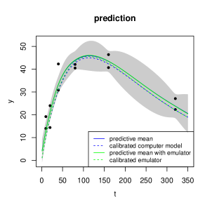
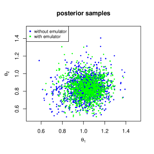
Figure 3: Comparison between Bayesian model calibration based on the numerical solver and the PP-GaSP emulator of the computer model. In the left panel, the green solid curve is the predictive mean by the calibrated computer model and discrepancy function, and the green dashed curves are predictions by the calibrated computer model alone, both of which call the numerical solver for each posterior sample. The same result based on the emulator is plotted as blue curves. The black dots are field observations and the shaded area is the interval $95\%$ predictive interval of the reality by the approach that uses the PP-GaSP emulator. In the right panel, posterior samples based on the numerical solver and the PP-GaSP emulator are plotted as green dots and blue dots, respectively.

Figure 3 gives predictions and posterior samples based on the numerical solver and the PP-GaSP emulator. First, the discrepancy (modeled by a S-GaSP) in both approaches looks to be very small, as predictive mean by the calibrated computer model and discrepancy function, and by the calibrated computer model are very close to each other. Second, predictions and posterior distributions by the numerical solver and by the emulator are almost the same for this example. Typically the emulator approach is preferred, as it is much faster than numerically solving differential equations for each posterior sample.

Calibration with multiple sources of observations

In reality, one may have observations of different types and they may come from multiple sources. For instance, satellite radar interferogram, observations from GPS stations, and tiltmeter observations are used to estimate the geological processes of volcanic eruption in Anderson et al. (2019). Multiple satellite interferograms are sometimes available for inference (Agram and Simons, 2015).

Bayesian model calibration using multiple sources of observations was discussed in Gu et al. (2022a). For each source $l$, $l=1,2,...,k$, let the field observations of the $l$ th source at observable input $\mathbf{x}$ be modeled as

$$\mathbf{y}^{F}_{l}(\mathbf{x})=f^{M}_{l}(\mathbf{x},\bm{\theta})+\delta(\mathbf{x})+\delta_{l}(\mathbf{x})+\mu_{l}+\epsilon_{l},$$ (14)

where $f^{M}_{l}(\mathbf{x},\bm{\theta})$ is the computer model for source $l$. The discrepancy function is denoted as $\delta(\mathbf{x})$ and the source-specific measurement bias is denoted as $\delta_{l}(\mathbf{x})$ , which are the correlated noise terms. Measurement bias often appear at satellite radar interferogram, as atmospheric error could affect the quality of the image. The mean (or trend) of each data source is denoted as $\mu_{l}$, and the independent measurement noise is denoted as $\epsilon_{l}$.

In RobustCalibration, we allow users to integrate observations from multiple sources to calibrate computer models by the function rcalibration_MS and to make predictions using the function predict_MS.rcalibration_MS. Posterior sampling method is implemented for parameter estimation for multiple sources of data. Besides, both GaSP and S-GaSP model can be chosen to model the measurement bias $\delta_{l}$, for $l=1,...,k$. Similar to calibration model with a single source of data, we allow users to choose a model with no-discrepancy, and with GaSP or S-GaSP model of the discrepancy function $\delta$. Users can choose to have measurement bias or not. Finally, we allows users to integrate different types of measurements for model calibration by using different designs of observable inputs.

An overview of RobustCalibration

Main functions

RobustCalibration package can be used for estimating the unobservable parameters from the computer models and for predicting the reality. Two key functions for calibrating computer models with a single type or source of field observations are rcalibration and predict.rcalibration. The function rcalibration allows user to call a posterior sampling algorithm and a numerical optimization algorithm for computing the MLE for parameter estimation. Additional arguments, such as handling observations from repeated experiments, choice of different discrepancy function, trend, and building a surrogate model for approximating computationally expensive computer models will be introduced in the next subsection. The rcalibration function returns an object of the rcalibration S4 class with posterior samples or MLE of parameters, including calibration parameters, trend parameters, noise in field observations, range and nugget parameters, to perform predictions. Then rcalibration S4 class is used as the input in the predict.rcalibration function to perform predictions on a set of test inputs. The predict.rcalibration function returns predictobj.rcalibration S4 class, which contains the predictive mean of calibrated computer model, estimated trend and discrepancy function. The estimated interval at any given range can also be output by specifying a vector of the interval_est argument in predict.raclibration function.

In some applications, we have different sources or types of observations. E.g. in calibrating geophysical model, time series of continuous GPS observations and satellite radar interferogram can be used jointly for estimating unobservable parameters (Anderson et al., 2019). Data from multiple sources can have different observable input. In RobustCalibration package, we implement parameter estimation for observations from multiple sources by the rcalibration_MS function, which returns a rcalibration_MS S4 class that contains posterior samples or MLE of parameters. The rcalibration_MS class can be used as an input into the predict_MS.rcalibration_MS function for predicting the reality.

The rcalibration function

The rcalibration function is the most important function in RobustCalibration package, as it performs parameter estimation for data inversion. To use this function, The following arguments in the rcalibration function are required: 1) an $n\times p_{x}$ matrix of observable inputs ($\mathbf{x}$) through argument design, 2) field observations ($\mathbf{y}^{F}$) by argument observations, 3) a $p_{\theta}\times 2$ matrix of containing the lower and upper bounds of calibration parameters ($\bm{\theta}$) by argument theta_range, where each row contains the lower and upper bound of the parameter values, and 4) a mathematical model specified by math_model or simulation runs by input_simul and output_simul for building the emulator. The RobustCalibration package can handle three different kinds of field observations by argument observations. First, one can input a n-vector $(y^{F}(\mathbf{x}_{1}),...,y^{F}(\mathbf{x}_{n}))^{T}$ into observations, when one field datum is available at each observable input. Second when $k$ repeated measurements are available for each observable input, one can input an $n\times k$ matrix of field observations, where each row contains $k$ replicates for one observable input. Third, one can also input a list, where each element contains $k_{i}$ replications at the $i$th observable input, for $i=1,...,n$.

An important feature of the RobustCalibration package is flexible specification of the computer model. The user can specify a mathematical model by giving a function in R through the argument math_model, and by selecting the default choice of the simulator simul_type=0. The second choice is to use an emulator to approximate the computer model by choosing simul_type=1. Users needs to input a small set of simulation runs by input_simul and output_simul to call an emulator by the RobustGaSP package. Users can give an $(p_{x}+p_{\theta})\times D$ matrix of input and a $D$-vector of output into input_simul and output_simul arguments. Then the rgasp from RobustGaSP function will be called to emulate the computer model. Or input_simul and output_simul arguments can be specified as a $p_{\theta}\times D$ matrix of input and a $p_{x}\times D$ matrix of output, such that ppgasp function from RobustGaSP will be called to emulate the computer model with $p_{\theta}$ dimension. To account for stochastic error or numerical approximation error in the simulator, we also allow users to specify a nugget parameter estimated by the simulator data by the argument simul_nug=T.

The rcalibration function contains many other user-specific arguments for applications in different scenarios. First, users can specify discrepancy models by GaSP and S-GaSP by the argument discrepancy_type=‘GaSP’ and discrepancy_type=‘S-GaSP’, respectively. The default choice is to assume a discrepancy model by S-GaSP. The model without a discrepancy can be specified by the argument discrepancy_type=‘no-discrepancy’. Second. for the model with or without a discrepancy function, the trend can be specified by the argument X. By default, the trend (or mean) of the calibration model is zero. Third, the parameter estimation approach can be specified by the method argument. The default choice is method=‘post_sample’ where posterior samples will be drawn, and stored in the slot post_sample of the rcalibration class created by the rcalibration function. The MLE can be specified by the argument method=‘mle’, and the estimated parameters are stored in the slot param_est of rcalibration class. Users can specify the number of MCMC samples by the argument S and S_0 for the total number of samples and the number of burn-in samples. The standard deviation of the proposal distribution for calibration parameters, the logarithm of the inverse range parameters and logarithm of the nugget parameter can be specified by the sd_proposal argument. Furthermore, users can thin their MCMC samples and only record a subset by the argument thinning. For instance, thinning=5 means only 1/5 of the posterior samples will be recorded. Users can adjust the roughness parameter in the power exponential kernel by the argument alpha and different prior parameters in the JR prior can be specified by arguments a and b. Besides, the inverse variance of measurement error of field observations at each observable input can be taken into consideration by the output_weights. Finally, arguments initial_values and num_initial_starts can be specified in numerical optimization to find MLE, and when the user use posterior sampling method, they can specify the initial values of the calibration parameters in MCMC through the argument initial_values.

The object rcalibration created by the rcalibration function have a few key elements. First of all, if we have method=’post_sample’, the after burn-in posterior samples of parameters will be stored in the slot post_sample, where each row contains a posterior draw. The first $p_{\theta}$ columns contain posterior samples of calibration parameters $\bm{\theta}$. In no-discrepancy calibration, the $p_{\theta}+1$ column of post_sample contains posterior draws of the noise variance $\sigma^{2}_{0}$ and the $p_{\theta}+2$ to $p_{\theta}+q+1$ columns contain the trend parameters $\bm{\theta}_{m}$, if the trend (X) is not a zero vector. In GaSP or S-GaSP calibration, the $p_{\theta}+1$ to $p_{\theta}+p_{x}+1$ columns record posterior draws of the log inverse range and log nugget parameters. The $p_{\theta}+p_{x}+2$ to $p_{\theta}+p_{x}+q$ column record the noise variance parameter and trend parameters if they are specified. The parameter $\lambda_{z}$ in S-GaSP are recorded in slots post_value and lambda_z, respectively. The indices of the accepted proposed samples are recorded in slots accept_S as one of the diagnostic statistics.

The predict.rcalibration function

After calling the rcalibration function, a rcalibration S4 class will be created, and it can be used as an input into the predict.rcalibration function for predicting the reality on a specified matrix of test input using the argument testing_input. Besides, if the trend basis X in rcalibration function was specified, we request the users to specify the trend basis of reality at test inputs by the argument X_testing in function predict.rcalibration. If the emulator was not constructed in rcalibration, users also need to specify the mathematical model by argument math_model in predict.rcalibration. Finally, the predictive interval can be specified by the argument interval_est. For instance, the 95% predictive interval can be obtained by the interval_est=c(0.025,0.975) argument. The interval of the field data that includes the estimated noise of field observations will be computed, if interval_data=T. Otherwise, the predictive interval of the reality will be computed. Finally, if the size of the noises in field data was specified by the output_weights, the users can also specify the variance of test data by testing_output_weights, which affects the predictive interval of test data.

After calling predict.rcalibration function, an object predictobj.rcalibration will be created that contains three different predictors for reality. The slot math_model_mean_no_trend gives the predictive mean based on calibrated computer model ($f^{M}$). The slot math_model_mean gives the predictive mean based on the calibrated computer model and estimated trend ($f^{M}+\mu$), if trend basis functions at observable input and test input are specified through X and X_testing in rcalibration and rcalibration.predict, respectively. The slot mean gives the predictive mean based on calibrated computer model, estimated trend and discrepancy ($f^{M}+\mu+\delta$). The predictive mean is typically more accurate for predicting the reality than using the computer model alone. Furthermore, if the predictive interval can be specified using the argument interval_est for uncertainty assessment of predictions. For instance, interval_est=c(0.025,0.975) means the $95\%$ interval will be computed.

The rcalibration_MS function and the predict_MS.rcalibration_MS function

Model calibration and predictions using multiple sources of data or different types of data are implemented by rcalibration_MS and rcalibration_MS.predict_MS functions, respectively. One only need to specify 3 components: design, observations, theta_range and a form of mathematical model. Suppose we have a data set from $k$ sources of observations. The design is a list of $k$ elements, where each element is a matrix of observable input for each source (or each type) of observations. The argument observations takes a list of field observations, where each element is a vector of field observations for each source. In principle, one can have different number of observations from each source and the type may not be the same. The argument theta_range is a $p_{\theta}\times 2$ matrix of the range of parameters, where each row $i$ contain the minimum and maximum values of the $i$th coordinate of calibration parameter $\bm{\theta}$. Furthermore, if closed form expressions of mathematical models are available for each source of data, users can input a list of functions into the math_model . We also allow users to emulate the expensive simulation. In this scenario, one needs to let simul_type be a vector of $1$s, indicating emulators will be called for each computer model.

Users can specify various arguments in rcalibration_MS. For instance, the argument index_theta takes a list of indices for the associated calibration parameter for each computer model. For instance, suppose we have $\bm{\theta}=(\theta_{1},\theta_{2},\theta_{3})$, and the computer model for first source of data is related to the first two calibration parameters and the computer model for second source of data is related to second two calibration parameters. Then index_theta is a list where index_theta[[1]]=c(1,2), and index_theta[[2]]=c(2,3). Furthermore, the measurement_bias is a bool value to include a measurement bias or not. If measurement_bias=T, then equation (14) is needed and the observable for $\delta$ is given in the shared_design argument. If measurement_bias=T, then $\delta=0$ and each $\delta_{i}$ is the discrepancy or correlated error for computer model for source $i$, for $i=1,...,k$. Similar to model calibration with single source of data, one can specify the type of discrepancy and kernel function of the discrepancy by discrepancy_type and kernel_type. Other arguments in rcalibration_MS are similar to rcalibration. After calling rcalibration_MS, an S4 class rcalibration_MS will be built, and used as an input to predict_MS.rcalibration_MS for making predictions.

Additional examples

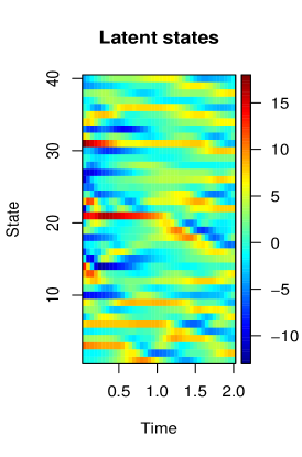
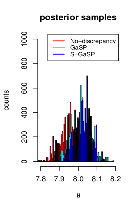
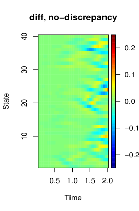
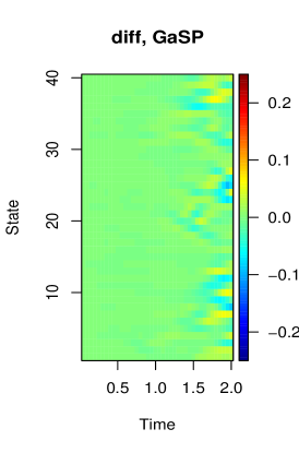
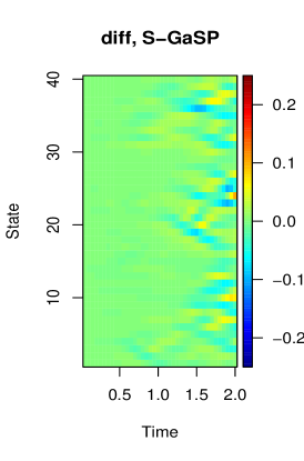
Figure 4: The reality and full observations of Lorenz-96 system in Scenario 1 are plotted at the upper left panel and upper middle panel, respectively, where the black circles are the $5\%$ observations used for model calibration. Posterior samples of calibration parameters of different calibration methods are plotted in the upper right panel. The lower panels give the difference between the reality and calibrated computer model of all latent states.

Model calibration for the Lorenz-96 system

Here we discuss an example of the Lorenz-96 system used in modeling atmospheric dynamics (Lorenz, 1996). The mathematical model is written as ODEs below:

$$\dot{x}_{j}(t)=(x_{j+1}(t)-x_{j-2}(t))x_{j-1}(t)-x_{j}(t)+\theta,$$ (15)

for $j=1,...,k$ states, with $k=40$ and $\theta$ is a scalar value of the force. Further assume that $x_{-1}=x_{k-1}$, $x_{0}=x_{k}$ and $x_{k+1}=x_{1}$ for any $t$. The latent variables $x_{i}$ can model the atmospheric quantities, such as temperature or pressure, measured at $k$ positions along a constant latitude circle. This model is widely used for data assimilation (Maclean and Spiller, 2020; Brajard et al., 2020).

We consider model calibration at two scenarios:

$$\mbox{Scenario 1: }\quad\quad\quad\quad\quad\quad\quad\quad\quad\quad y_{j}(t) =x_{j}(t)+\epsilon,\quad\quad\quad\quad\quad\quad\quad\quad\quad\quad\quad\quad$$ (16)

$$\mbox{Scenario 2: }\quad\quad\quad\quad\quad\quad\quad\quad\quad\quad y_{j}(t) =x_{j}(t)+2t\sin\left(\frac{2\pi j}{k}\right)+\epsilon,\quad\quad\quad\quad\quad\quad\quad\quad\quad\quad\quad\quad$$ (17)

for $j=1,...,k$ and $\epsilon\sim N(0,1)$ is an in dependent Gaussian noise. In the first scenario, the mathematical model is a true model and in the second scenario, a discrepancy term is included for simulating the field data. The discrepancy is treated unknown. We initialize the states by a multivariate normal with the covariance generated from a Wishart distribution with $k$ degrees of freedom and a diagonal scale matrix. We use the Runge Kutta method with order 4 to numerically solve the systems. Since the computer model is fast, we do not include an emulator. We simulate the reality at $40$ time points, with time step $0.05$ between them.

The unobserved reality simulated by the Lorenz-96 system is plotted in upper model panel in Figure 4. Only $5\%$ observations (i.e. 2 observations at each time point, graphed as black circles in upper middle panel) are available for model calibration. The posterior parameters of no-discrepancy calibration, GaSP and S-GaSP calibration are graphed in the upper right panels. Note that here since the computer model (Lorenz-96) is the true model, the no-discrepancy calibration is expected to perform well. Even though one allows a flexible discrepancy function, modeled as GaSP or S-GaSP, it seems parameters are estimated reasonably well in both approach. In all methods, posterior samples are centered around the true parameter ($\theta=8$), and the range of posterior samples is short compared to the parameter range $[-20,20]^{2}$. The estimate states by the calibrated computer model and the reality are plotted in the lower panels in Figure 4. All methods have small estimation errors, as the parameters are estimated well.

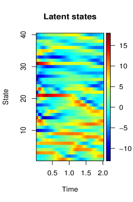
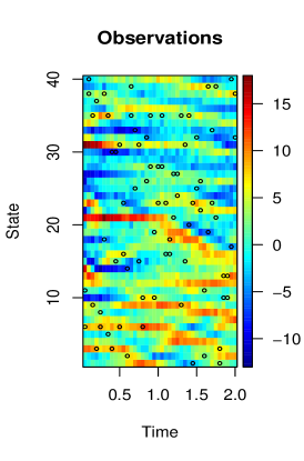
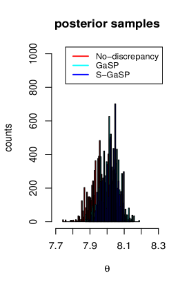
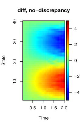
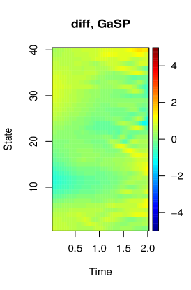
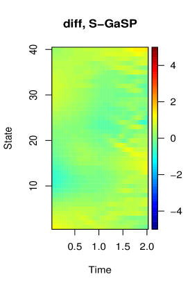
Figure 5: The reality of a discrepancy-included Lorenz-96 system (Scenario 2) is plotted at the upper left panel, The simulated observations are graphed at the upper middle panel, where the $5\%$ of the observations plotted as black circles are used in model calibration. Posterior samples of calibration parameters of different calibration methods are plotted at the upper right panel. The lower panels give the difference between the reality and calibrated computer model with discrepancy (if estimated) of all latent states.

The reality, observations, posterior samples and predictions from different calibration models for a discrepancy-included Lorenz-96 system are graphed in Figure 5. Note that since the discrepancy is included, there is no true calibration parameter. The estimated states by the no-discrepancy calibration model (shown in the lower left panel) has relatively large error. This is not surprising as the Lorenz-96 system is a misspecified model. The predictive mean of GaSP and S-GaSP by including both the calibrated computer model and discrepancy function are more accurate, as both model captures the discrepancy between the reality and computer model. Note that the estimation error of all models are larger than the ones when there is no discrepancy. This is because the measure error is large and we only observe 2 states at each time points. Increasing the number of observations or reducing the variance of measurement error can improve predictive accuracy.

Model calibration with multiple sources of data with a measurement bias

So far our example focus on model calibration with single source of data, with the use of rcalibration function for parameter estimation and predict function for predictions. In Anderson et al. (2019), for instance, multiple satellite interferogram and GPS observations measuring the ground deformation during the eruption of the Kīlauea volcano eruption in summer 2018 are used for calibration of mechanical model that relates the observations to calibration parameters, such as depth and shape of the magma chamber, magma density, pressure change rate and so on. In these applications, the measurement bias, such as atmospheric error, can substantially affect the satellite measurements of ground deformation (Zebker et al., 1997). The correlated measurement bias can be modeled as multivariate normal in each source of data (Gu et al., 2022a). Model calibration and predictions for scenarios with or without measurement bias have been implemented in the rcalibration_MS function and predict_MS function.

Here we introduce a simulated example for model calibration with multiple sources of data, such as multiple images or time series data. The $l$th source of data, $l=1,...,k$, is simulated by the equation below

$$y^{R}_{l}(x)=sin(\pi x)+\delta(x)+\delta_{l}(x)+\epsilon_{l}(x),$$ (18)

where $\delta(.)$ and $\delta(.)$ are independently simulated from Gaussian processes with covariance $\sigma^{2}K(.,.)$ and $\sigma^{2}_{l}K_{l}(\cdot,\cdot)$, and the independent noise follows $\epsilon_{l}(x)\overset{i.i.d}{\sim}N(0,\sigma^{2}_{0})$. We let $\sigma=0.05$, $\sigma=0.2$ and $\sigma^{2}_{l}=0.5+(1-0.5)/(k-1)$. The $K(.,.)$ and $K_{l}(\cdot,\cdot)$ are assumed to follow Matérn correlation with roughness parameter being $\alpha=2.5$, the range parameter being $\gamma=1/30$ and $\gamma=1/10$, respectively. We collect $n=100$ observations for each source $l$ with $x$ equally spaced from $[0,1]$. We assume data from $k=5$ sources are available. Here the mathematical model follows $f^{M}_{l}(x,\theta)=sin(\theta x)$, for $l=1,...,k$, and the reality is $y^{R}(x)=f^{M}_{l}(x,\theta)+\delta(x)$. The goal is to estimate the calibration parameter ($\theta$), the reality ($y^{R}(x)=f^{M}_{l}(x,\theta)+\delta(x)$), model discrepancy($\delta(x)$), and measurement bias ($\delta_{l}(x)$).

We compare four methods. The GaSP and S-GaSP are the calibration methods that model individual sources of data, with the discrepancy model specified as a GaSP and S-GaSP respectively. The measurement bias is assumed to model by GaSPs. Here since the observable inputs are overlapped, a common way is to use the aggregated or the stack data $\bar{y}^{R}(x)=\sum^{k}_{l=1}y^{R}_{l}(x)/k$ to calibrate the model, as the computation of modeling the aggregated data is around $k$ times faster than modeling the individual sources of data. We compare with two methods of modeling the aggregated data, namely the GaSP Stack and S-GaSP Stack, representing the scenario where the discrepancy model is specified as a GaSP or S-GaSP, respectively.

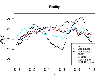
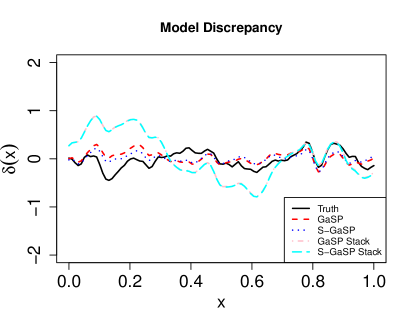
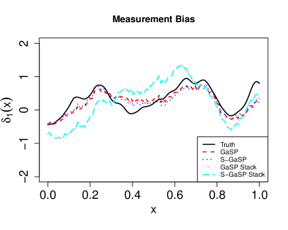
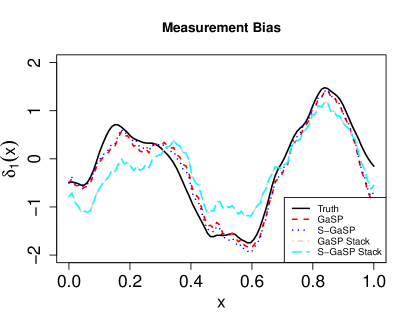
Figure 6: Model calibration comparison between modeling individual data and aggregated (averaged) data for simulation from Equation (18). The upper left and right panels give the reality and model discrepancy, whereas the lower two panels give the measurement bias for the first two sources. The estimation results from GaSP, S-GaSP, GaSP Stack and S-GaSP calibration are plotted as red, blue, pink and cyan curves. The observations from the first two sources are graphed as the triangles and dots in the upper left panel.

In Figure 6, we graph the truth, observations of the first two sources of observations, and estimation of reality, discrepancy and first two measurement bias from four different methods. Here the GaSP and S-GaSP perform better than the GaSP Stack and S-GaSP Stack calibration methods, as aggregating data causes the loss of information when the measurement bias presents. The RMSE of reality, discrepancy and measurement bias estimation of different methods are given in the Table 3.

RMSE	reality	discrepancy	measurement bias
GaSP	0.238	0.194	0.247
S-GaSP	0.204	0.159	0.214
GaSP Stack	0.501	0.483	0.504
S-GaSP Stack	0.502	0.484	0.504

Table 3: The RMSE of the reality, discrepancy and measurement bias, where the smaller number indicates a smaller error. For measurement bias, we average the RMSE for each source of data.

Finally, The mean of posterior samples $\theta$ from the GaSP, S-GaSP, GaSP Stack and S-GaSP Stack calibration for calibration parameter $\theta$ are 2.46, 2.73, 2.15, and 2.17 respectively, whereas the truth $\theta=\pi\approx 3.14$. This is a challenging scenario, as the large measurement bias makes estimation hard. We found model calibration by modeling individual sources of data is more accurate than modeling the aggregated data, whereas modeling the aggregated data is more computationally scalable.

Concluding remarks

We have introduced the RobustCalibration package for Bayesian model calibration and data inversion. This package has implemented a range estimation methods and models, such as posterior sampling and MLE, for no-discrepancy calibration, GaSP and S-GaSP models of the discrepancy function. We implement statistical emulators for approximating computationally expensive computer models with both scalar-valued output or vectorized output. The package is applicable to observations from a single source with or without replications, and to observations from multiple sources or having different types. We illustrate our approaches on mathematical models with closed-form expressions or written as differential equations.

Even if we tried our best to consider different possible scenarios, a comprehensive statistical package for model calibration and data inversion is an ambitious goal. The RobustCalibration package provide tools for people to perform Bayesian model inversion without the need to write emulator or MCMC samples themselves. We will keep improving RobustCalibration package towards a few directions. First and foremost, we will make this package more computationally scalable on structured data, such as imaging and time series observations. Second, for problems like the Lorzen-96 system, it may be important to emulate the time evolution operator, if forecasting is our goal. Furthermore, we will allow users to specify other prior of the parameters and proposal distributions for posterior samples in future versions of the package.

Appendix

Auxiliary facts

1. Let $\tilde{\bm{R}}_{\gamma,\eta}=\mathbf{R}_{\gamma}/\eta+\bm{\Lambda}$ be an $n\times n$ positive definite matrix as a function of parameters $\bm{\gamma}$ and $\eta$. Then for $l=1,...,p_{x}$

   $$\frac{\partial\log|\tilde{\bm{R}}_{\gamma,\eta}|}{\partial\gamma_{l}}=\operatorname{tr}\left(\frac{\tilde{\bm{R}}_{\gamma,\eta}^{-1}}{\eta}\frac{\partial\mathbf{R}_{\gamma}}{\partial\bm{\gamma}_{l}}\right)\quad\mbox{ and }\quad\frac{\partial\log|\tilde{\bm{R}}_{\gamma,\eta}|}{\partial\eta}=-\operatorname{tr}\left(\frac{\tilde{\bm{R}}_{\gamma,\eta}^{-1}\mathbf{R}_{\gamma}}{\eta^{2}}\right).$$

2. Let $\mathbf{H}$ be an $n\times q$ full rank matrix with $q<n$, $\mathbf{Q}=\left(\tilde{\bm{R}}^{-1}_{\gamma,\eta}-\tilde{\bm{R}}^{-1}_{\gamma,\eta}\mathbf{H}^{T}(\mathbf{H}^{T}\tilde{\bm{R}}^{-1}_{\gamma,\eta}\mathbf{H})^{-1}\mathbf{H}^{T}\tilde{\bm{R}}^{-1}_{\gamma,\eta}\right)$ with $\tilde{\bm{R}}_{\gamma,\eta}=\mathbf{R}_{\gamma}/\eta+\bm{\Lambda}$ and $\mathbf{y}$ is an $n\times 1$ vector. Then for $l=1,...,p_{x}$

   $$\frac{\partial\log(\mathbf{y}^{T}\mathbf{Q}_{\gamma,\eta}\mathbf{y})}{\partial\gamma_{l}}=-\frac{\mathbf{y}^{T}\mathbf{Q}_{\gamma,\eta}\frac{\partial\mathbf{R}_{\gamma}}{\partial\gamma_{l}}\mathbf{Q}_{\gamma,\eta}\mathbf{y}}{\eta\mathbf{y}^{T}\mathbf{Q}_{\gamma,\eta}\mathbf{y}}\quad\mbox{ and }\quad\frac{\partial\log(\mathbf{y}^{T}\mathbf{Q}_{\gamma,\eta}\mathbf{y})}{\partial\eta}=\frac{\mathbf{y}^{T}\mathbf{Q}_{\gamma,\eta}\mathbf{R}_{\gamma}\mathbf{Q}_{\gamma,\eta}\mathbf{y}}{\eta^{2}\mathbf{y}^{T}\mathbf{Q}_{\gamma,\eta}\mathbf{y}}.$$

3. Suppose $v_{\bm{\theta}}$ is an $n\times 1$ vector as a function of $\bm{\theta}$ and $\mathbf{\tilde{R}}$ is an $n\times n$ positive definite matrix. Then for $i=1,...,p_{\theta}$

   $$\frac{\partial\log(\mathbf{v}_{\bm{\theta}}^{T}\mathbf{R}^{-1}\mathbf{v}_{\bm{\theta}})}{\partial\theta_{l}}=\frac{2\mathbf{v}_{\theta}^{T}\mathbf{\tilde{R}}^{-1}\frac{\partial\mathbf{v}_{\theta}}{\partial\theta_{l}}}{\mathbf{v}^{T}_{\theta}\mathbf{\tilde{R}}^{-1}\mathbf{v}_{\theta}}.$$

Likelihood functions and posterior distributions

Posterior distribution of the no-discrepancy calibration. Using the objective prior for the mean and variance parameters, $\pi(\bm{\theta}_{m},\sigma^{2}_{0})\propto 1/\sigma^{2}_{0}$, full conditional posterior distributions of the trend and variance parameters follow

$$\sigma^{-2}_{0}\mid\bm{\theta}_{m},\bm{\theta} \sim\mbox{Gamma}\left(\frac{n}{2},\frac{(\mathbf{y}^{F}-\mathbf{f}^{M}_{\theta}-\mathbf{H}\bm{\theta}_{m})^{T}\bm{\Lambda}^{-1}(\mathbf{y}^{F}-\mathbf{f}^{M}_{\theta}-\mathbf{H}\bm{\theta}_{m})}{2}\right),$$

$$\bm{\theta}_{m}\mid\sigma^{2}_{0},\bm{\theta} \sim\mathcal{N}\left(\bm{\hat{\theta}}^{LS}_{m},\,\sigma^{-2}_{0}(\mathbf{H}^{T}\bm{\Lambda}^{-1}\mathbf{H})^{-1}\right).$$

The posterior distribution of the calibration parameters follows

$$p(\bm{\theta}\mid\bm{\theta}_{m},\bm{\sigma}^{2}_{0},\bm{\beta},\eta)\propto\exp\left(-\frac{(\mathbf{y}^{F}-\mathbf{f}^{M}_{\theta}-\mathbf{H}\bm{\theta}_{m})^{T}\bm{\Lambda}^{-1}(\mathbf{y}^{F}-\mathbf{f}^{M}_{\theta}-\mathbf{H}\bm{\theta}_{m})}{2\sigma^{2}_{0}}\right)\pi(\bm{\theta}),$$

where $\pi(\bm{\theta})$ is the prior of calibration parameters, where the default prior distribution is the uniform distribution $\pi(\bm{\theta})\propto 1$. We use a Metropolis algorithm to sample the calibration parameters. Here we sample all calibration parameters as a block, instead of sequentially, as we only need to compute the likelihood once in block sampling. The proposal distribution of each coordinate of the calibration parameter vector is chosen as a normal distribution with a pre-specified standard deviation proportional to the range of the parameters. The default proportion is $0.05$, and users can adjust the proportion by changing the first $p_{\theta}$ value in the argument sd_proposal in rcalibration function. If, for instance, the proportion of accepted calibration parameters is too low, one can reduce the first $p_{\theta}$ value in the argument sd_proposal to use a smaller standard deviation in the proposal distribution.

After obtaining $S$ posterior samples with the first $S_{0}$ burn-in samples, the predictive mean of reality based on calibrated computer model and trend by the no-discrepancy calibration can be computed by

$$\hat{\mu}(\mathbf{x}^{*})=\frac{1}{S-S_{0}}\sum^{S}_{i=S_{0}+1}f^{M}(\mathbf{x}^{*},{\bm{\theta}}^{(i)})+\mathbf{h}(\mathbf{x}^{*}){\bm{\theta}_{m}^{(i)}}.$$

The posterior credible interval of the reality $y^{R}(\mathbf{x}^{*})$ in no-discrepancy calibration can be obtained by the empirical quantile of posterior samples $f^{M}(\mathbf{x}^{*},{\bm{\theta}}^{(i)})+\mathbf{h}(\mathbf{x}^{*}){\bm{\theta}_{m}^{(i)}}$. For example, the posterior credible interval of $1-\alpha$ percentile of the data $f^{M}(\mathbf{x}^{*})$ in no-discrepancy calibration can be computed by

$$\frac{1}{S-S_{0}}\sum^{S}_{i=S_{0}+1}f^{M}(\mathbf{x}^{*},{\bm{\theta}}^{(i)})+\mathbf{h}(\mathbf{x}^{*}){\bm{\theta}_{m}^{(i)}}+\sqrt{\frac{\sigma^{(i)}_{0}}{w^{*}}}Z_{\alpha},$$

where $Z_{\alpha}$ is an upper $\alpha$ quantile of the standard normal distribution and $w^{*}$ is the relative test output weight (assumed to be 1 by default).

Likelihood function and derivatives in GaSP calibration. The profile likelihood function in GaSP calibration follows

$$\mathcal{L}_{K}(\bm{\theta},\bm{\gamma},\eta\mid{\hat{\bm{\theta}}_{m}},\hat{\sigma}^{2}_{0})\propto|{\mathbf{\tilde{R}}}|^{-\frac{1}{2}}(S^{2}_{K})^{-\frac{n}{2}},$$ (19)

where $S^{2}_{K}=(\mathbf{y}-\mathbf{f}^{M}_{\theta}-\mathbf{H}^{T}\hat{\bm{\theta}}_{m})^{T}{{\mathbf{\tilde{R}}}}^{-1}(\mathbf{y}-\mathbf{f}^{M}_{\theta}-\mathbf{H}^{T}\hat{\bm{\theta}}_{m})$.

Denote $\mathbf{v}_{\bm{\theta}_{m}}:=(\mathbf{y}-\mathbf{f}^{M}_{\theta}-\mathbf{H}^{T}\hat{\bm{\theta}}_{m})$. Similar to the no-discrepancy calibration, we call the lbfgs function in the nloptr package (Ypma (2014)) for optimization. By facts 1 and 3, directly differentiating the profile likelihood function with respect to kernel and nugget parameters in (19) gives:

$$\frac{\partial\log(\mathcal{L}_{K}(\bm{\theta},\bm{\gamma},\eta,\mid{\bm{\hat{}}\theta_{m}},\hat{\sigma}^{2}))}{\partial\bm{\gamma}_{l}} =-\frac{1}{2}\operatorname{tr}\left(\frac{\tilde{\bm{R}}_{\gamma,\eta}^{-1}}{\eta}\frac{\partial\mathbf{R}_{\gamma}}{\partial\bm{\gamma}_{l}}\right)+\frac{n}{2}\times\frac{\mathbf{v}_{\bm{\theta}_{m}}^{T}\mathbf{Q}_{\gamma,\eta}\frac{\partial\mathbf{R}_{\gamma}}{\partial\gamma_{l}}\mathbf{Q}_{\gamma,\eta}\mathbf{v}_{\bm{\theta}_{m}}}{\eta\mathbf{v}_{\bm{\theta}_{m}}^{T}\mathbf{Q}_{\gamma,\eta}\mathbf{v}_{\bm{\theta}_{m}}}$$

$$\frac{\partial\log(\mathcal{L}_{K}(\bm{\theta},\bm{\gamma},\eta,\mid{\bm{\hat{}}\theta_{m}},\hat{\sigma}^{2}))}{\partial\eta} =\frac{1}{2}\operatorname{tr}\left(\frac{\tilde{\bm{R}}_{\gamma,\eta}^{-1}\mathbf{R}_{\gamma}}{\eta^{2}}\right)+\frac{n}{2}\times\frac{\mathbf{v}_{\bm{\theta}_{m}}^{T}\mathbf{Q}_{\gamma,\eta}\mathbf{R}_{\gamma}\mathbf{Q}_{\gamma,\eta}\mathbf{v}_{\bm{\theta}_{m}}}{\eta^{2}\mathbf{v}_{\bm{\theta}_{m}}^{T}\mathbf{Q}_{\gamma,\eta}\mathbf{v}_{\bm{\theta}_{m}}}$$

$$\frac{\partial\log(\mathcal{L}_{K}(\bm{\theta},\bm{\gamma},\eta,\mid{\bm{\hat{}}\theta_{m}},\hat{\sigma}^{2}))}{\partial\theta_{l}} =\frac{n}{2}\times\frac{\mathbf{v}_{\bm{\theta}_{m}}^{T}\mathbf{Q}_{\gamma,\eta}\frac{\partial\mathbf{f}^{M}_{\theta}}{\partial\theta_{l}}}{\mathbf{v}_{\bm{\theta}_{m}}^{T}\mathbf{Q}_{\gamma,\eta}\mathbf{v}_{\bm{\theta}_{m}}}$$

for $l=1,...,p_{x}$ and $i=1,...,p_{\theta}$. When the mean function is zero, one can simply replace $\mathbf{Q}_{\gamma,\eta}$ by $\tilde{\bm{R}}_{\gamma,\eta}$ in the formula above to obtain the derivatives. Besides, when $\frac{\partial\mathbf{f}^{M}_{\theta}}{\partial\theta_{l}}$ is not available, we use the numerical derivatives to approximate.

Posterior distributions in GaSP calibration. After marginalizing out the discrepancy function, the marginal distribution follows $\mathbf{y}^{F}\sim\mathcal{MN}(\mathbf{f}^{M}_{\theta}+\mathbf{H}\bm{\theta}_{m},\,\sigma^{2}_{0}\tilde{\mathbf{R}})$, where $\tilde{\mathbf{R}}=\mathbf{R}/\eta+\bm{\Lambda}$. We assume the object prior for the mean and noise variance parameters $\pi(\bm{\theta}_{m},\sigma^{2}_{0})\propto 1/\sigma^{2}_{0}$. Full conditional posterior distributions of the trend and variance parameters follow

$$\bm{\sigma}^{-2}_{0}\mid\bm{\theta}_{m},\bm{\theta} \sim\mbox{Gamma}\left(\frac{n}{2},\frac{(\mathbf{y}^{F}-\mathbf{f}^{M}_{\theta}-\mathbf{H}\bm{\theta}_{m})^{T}\bm{\tilde{R}}^{-1}(\mathbf{y}^{F}-\mathbf{f}^{M}_{\theta}-\mathbf{H}\bm{\theta}_{m})}{2}\right),$$

$$\bm{\theta}_{m}\mid\sigma^{2}_{0},\bm{\theta} \sim\mathcal{MN}\left(\bm{\hat{\theta}}_{m},\,\sigma^{-2}_{0}(\mathbf{H}^{T}\bm{\tilde{R}}^{-1}\mathbf{H})^{-1}\right),$$

where $\hat{\bm{\theta}}_{m}=\left(\mathbf{H}^{T}{{\mathbf{\tilde{R}}}}^{-1}\mathbf{H}\right)^{-1}\mathbf{H}^{T}{{\mathbf{\tilde{R}}}}^{-1}{(\mathbf{y}-\mathbf{f}^{M}_{\theta})}$. Since the full conditional distributions are known, a Gibbs sampler is used to sample $\bm{\sigma}^{-2}_{0}$ and $\bm{\theta}_{m}$ from the full conditional distribution.

Given the trend and variance parameter, the conditional distribution of the calibration parameters follows

$$p(\bm{\theta}\mid\bm{\theta}_{m},\bm{\sigma}^{2})\propto\exp\left(-\frac{(\mathbf{y}^{F}-\mathbf{f}^{M}_{\theta}-\mathbf{H}\bm{\theta}_{m})^{T}\mathbf{\tilde{R}}^{-1}(\mathbf{y}^{F}-\mathbf{f}^{M}_{\theta}-\mathbf{H}\bm{\theta}_{m})}{2\sigma^{2}_{0}}\right)\pi(\bm{\theta}),$$

We implement the Metropolis algorithm with the proposal distribution being a normal distribution with the mean centered around the current value of the posterior sample. Users can adjust the standard deviation of the proposal distribution by argument sd_proposal in the rcalibration function.

Denote the inverse range parameter $\beta_{l}=1/\gamma_{l}$, $l=1,...,p_{x}$. The conditional distribution of the inverse range and nugget parameters follow

$$p(\bm{\beta},\eta\mid\bm{\theta},\bm{\theta}_{m},\bm{\sigma}^{2}_{0})\propto|\mathbf{\tilde{R}}|^{-\frac{n}{2}}\exp\left(-\frac{(\mathbf{y}^{F}-\mathbf{f}^{M}_{\theta}-\mathbf{H}\bm{\theta}_{m})^{T}\mathbf{\tilde{R}}^{-1}(\mathbf{y}^{F}-\mathbf{f}^{M}_{\theta}-\mathbf{H}\bm{\theta}_{m})}{2\sigma^{2}_{0}}\right)\pi(\bm{\gamma},\eta),$$

where we assume the prior for the range and nugget parameters follows the jointly robust (JR) prior (Gu, 2019)

$$\pi(\bm{\beta},\eta)=C\left(\sum^{p_{x}}_{l=1}C_{l}\beta_{l}+\eta\right)^{a}\exp\left\{-b\left(\sum^{p_{x}}_{l}C_{l}\beta_{l}+\eta\right)\right\}$$

where $C$ is normalizing constant. By default, we use the following prior parameters $a=1/2-p_{x}$, $b=1$, and $C_{l}=n^{-1/{p_{x}}}|x^{max}_{l}-x^{min}_{l}|$, with $x^{max}_{l}$ and $x^{min}_{l}$ being the maximum and minimum values of the observable input at the $l$th coordinate. Users can adjust $a$ and $b$ in the rcalibration function. The JR prior is a proper prior. Furthermore, the default choices of prior parameters induces a small penalty on very large correlation, preventing the identifiability issues of the calibration parameters due to large correlation (Gu, 2019).

Since the posterior distribution is not a known distribution, we use the Metropolis algorithm to sample the logarithm of the inverse range parameter $\log(\bm{\beta})$ and nugget parameter $\log(\eta)$. The proposal distribution of each parameter is a normal distribution centered around the current value and with a pre-specified standard deviation chosen to be $0.25$ by default. User can change the $p_{\theta}+1$ to $p_{x}+p_{\theta}+1$ coordinates of the vector in the argument sd_proposal in the rcalibration function to specify the standard deviation in the proposal distribution for these parameters.

Likelihood function and posterior distributions S-GaSP calibration. The likelihood function and posterior distribution of S-GaSP follow from the those in GaSP calibration, by simply replacing the kernel $K$ to $K_{Z_{d}}$ in Table 1.

Mengyang Gu
Department of Statistics and Applied Probability
University of California, Santa Barbara
Santa Barbara, California, USA
mengyang@pstat.ucsb.edu

References

- Agram and Simons (2015) P. Agram and M. Simons. A noise model for InSAR time series. Journal of Geophysical Research: Solid Earth, 120(4):2752–2771, 2015.
- Anderson et al. (2019) K. R. Anderson, I. A. Johanson, M. R. Patrick, M. Gu, P. Segall, M. P. Poland, E. K. Montgomery-Brown, and A. Miklius. Magma reservoir failure and the onset of caldera collapse at Kīlauea volcano in 2018. Science, 366(6470), 2019.
- Arendt et al. (2012) P. D. Arendt, D. W. Apley, and W. Chen. Quantification of model uncertainty: calibration, model discrepancy, and identifiability. Journal of Mechanical Design, 134(10):100908, 2012.
- Bayarri et al. (2007a) M. Bayarri, J. Berger, J. Cafeo, G. Garcia-Donato, F. Liu, J. Palomo, R. Parthasarathy, R. Paulo, J. Sacks, and D. Walsh. Computer model validation with functional output. The Annals of Statistics, 35(5):1874–1906, 2007a.
- Bayarri et al. (2007b) M. J. Bayarri, J. O. Berger, R. Paulo, J. Sacks, J. A. Cafeo, J. Cavendish, C.-H. Lin, and J. Tu. A framework for validation of computer models. Technometrics, 49(2):138–154, 2007b.
- Box and Coutie (1956) G. Box and G. Coutie. Application of digital computers in the exploration of functional relationships. Proceedings of the IEE-Part B: Radio and Electronic Engineering, 103(1S):100–107, 1956.
- Brajard et al. (2020) J. Brajard, A. Carrassi, M. Bocquet, and L. Bertino. Combining data assimilation and machine learning to emulate a dynamical model from sparse and noisy observations: A case study with the Lorenz 96 model. Journal of Computational Science, 44:101171, 2020.
- Carmassi et al. (2018) M. Carmassi, P. Barbillon, M. Chiodetti, M. Keller, and E. Parent. Calico: a r package for bayesian calibration. arXiv preprint arXiv:1808.01932, 2018.
- Chang et al. (2016) W. Chang, M. Haran, P. Applegate, and D. Pollard. Calibrating an ice sheet model using high-dimensional binary spatial data. Journal of the American Statistical Association, 111(513):57–72, 2016.
- Chang et al. (2022) W. Chang, B. A. Konomi, G. Karagiannis, Y. Guan, and M. Haran. Ice model calibration using semicontinuous spatial data. The Annals of Applied Statistics, 16(3):1937–1961, 2022.
- Gu (2019) M. Gu. Jointly robust prior for Gaussian stochastic process in emulation, calibration and variable selection. Bayesian Analysis, 14(1), 2019.
- Gu and Wang (2018) M. Gu and L. Wang. Scaled Gaussian stochastic process for computer model calibration and prediction. SIAM/ASA Journal on Uncertainty Quantification, 6(4):1555–1583, 2018.
- Gu et al. (2019) M. Gu, J. Palomo, and J. O. Berger. RobustGaSP: Robust Gaussian Stochastic Process Emulation in R. The R Journal, 2019.
- Gu et al. (2022a) M. Gu, K. Anderson, and E. McPhillips. Calibration of imperfect mathematical models by multiple sources of data with measurement bias. arXiv preprint arXiv:1810.11664, 2022a.
- Gu et al. (2022b) M. Gu, F. Xie, and L. Wang. A theoretical framework of the scaled Gaussian stochastic process in prediction and calibration. SIAM/ASA Journal of Uncertainty Quantification, In Press, arXiv preprint arXiv:1807.03829, 2022b.
- Hankin (2005) R. K. Hankin. Introducing BACCO, an R bundle for Bayesian analysis of computer code output. Journal of Statistical Software, 14:1–21, 2005.
- Higdon et al. (2008) D. Higdon, J. Gattiker, B. Williams, and M. Rightley. Computer model calibration using high-dimensional output. Journal of the American Statistical Association, 103(482):570–583, 2008.
- Kennedy and O’Hagan (2001) M. C. Kennedy and A. O’Hagan. Bayesian calibration of computer models. Journal of the Royal Statistical Society: Series B (Statistical Methodology), 63(3):425–464, 2001.
- Liu and Nocedal (1989) D. C. Liu and J. Nocedal. On the limited memory bfgs method for large scale optimization. Mathematical programming, 45(1-3):503–528, 1989.
- Liu et al. (2009) F. Liu, M. Bayarri, and J. Berger. Modularization in Bayesian analysis, with emphasis on analysis of computer models. Bayesian Analysis, 4(1):119–150, 2009.
- Lorenz (1996) E. N. Lorenz. Predictability: A problem partly solved. In Proc. Seminar on predictability, volume 1, 1996.
- Ma et al. (2019) P. Ma, G. Karagiannis, B. A. Konomi, T. G. Asher, G. R. Toro, and A. T. Cox. Multifidelity computer model emulation with high-dimensional output: An application to storm surge. arXiv preprint arXiv:1909.01836, 2019.
- MacDonald et al. (2015) B. MacDonald, P. Ranjan, H. Chipman, et al. Gpfit: An R package for fitting a Gaussian process model to deterministic simulator outputs. Journal of Statistical Software, 64(i12), 2015.
- Maclean and Spiller (2020) J. Maclean and E. T. Spiller. A surrogate-based approach to nonlinear, non-Gaussian joint state-parameter data assimilation. arXiv preprint arXiv:2012.04793, 2020.
- Nocedal (1980) J. Nocedal. Updating quasi-Newton matrices with limited storage. Mathematics of computation, 35(151):773–782, 1980.
- Palomo et al. (2015) J. Palomo, R. Paulo, G. García-Donato, et al. Save: an R package for the statistical analysis of computer models. Journal of Statistical Software, 64(13):1–23, 2015.
- Paulo et al. (2012) R. Paulo, G. García-Donato, and J. Palomo. Calibration of computer models with multivariate output. Computational Statistics and Data Analysis, 56(12):3959–3974, 2012.
- Plumlee (2017) M. Plumlee. Bayesian calibration of inexact computer models. Journal of the American Statistical Association, 112(519):1274–1285, 2017.
- Roustant et al. (2012) O. Roustant, D. Ginsbourger, and Y. Deville. Dicekriging, Diceoptim: Two R packages for the analysis of computer experiments by kriging-based metamodeling and optimization. Journal of Statistical Software, 51(1):1–55, 2012. ISSN 1548-7660.
- Sacks et al. (1989) J. Sacks, W. J. Welch, T. J. Mitchell, H. P. Wynn, et al. Design and analysis of computer experiments. Statistical science, 4(4):409–423, 1989.
- Santner et al. (2003) T. J. Santner, B. J. Williams, and W. I. Notz. The design and analysis of computer experiments. Springer Science & Business Media, 2003.
- Simakov et al. (2019) N. A. Simakov, R. L. Jones-Ivey, A. Akhavan-Safaei, H. Aghakhani, M. D. Jones, and A. K. Patra. Modernizing titan2d, a parallel amr geophysical flow code to support multiple rheologies and extendability. In International Conference on High Performance Computing, pages 101–112. Springer, 2019.
- Soetaert et al. (2010) K. Soetaert, T. Petzoldt, and R. W. Setzer. Solving differential equations in R: package desolve. Journal of statistical software, 33:1–25, 2010.
- Tuo and Wu (2015) R. Tuo and C. J. Wu. Efficient calibration for imperfect computer models. The Annals of Statistics, 43(6):2331–2352, 2015.
- Wickham (2011) H. Wickham. ggplot2. Wiley Interdisciplinary Reviews: Computational Statistics, 3(2):180–185, 2011.
- Williamson et al. (2013) D. Williamson, M. Goldstein, L. Allison, A. Blaker, P. Challenor, L. Jackson, and K. Yamazaki. History matching for exploring and reducing climate model parameter space using observations and a large perturbed physics ensemble. Climate dynamics, 41(7-8):1703–1729, 2013.
- Wong et al. (2017) R. K. Wong, C. B. Storlie, and T. Lee. A frequentist approach to computer model calibration. Journal of the Royal Statistical Society: Series B (Statistical Methodology), 79:635–648, 2017.
- Ypma (2014) J. Ypma. nloptr: R interface to NLopt, 2014. URL https://CRAN.R-project.org/package=nloptr. R package version 1.0.4.
- Zebker et al. (1997) H. A. Zebker, P. A. Rosen, and S. Hensley. Atmospheric effects in interferometric synthetic aperture radar surface deformation and topographic maps. Journal of Geophysical Research: Solid Earth, 102(B4):7547–7563, apr 1997. ISSN 01480227. doi: 10.1029/96JB03804. URL http://doi.wiley.com/10.1029/96JB03804.