A non-perturbative study of the interplay between electron-phonon interaction and Coulomb interaction in undoped graphene

Abstract

In condensed-matter systems, electrons are subjected to two different interactions under certain conditions. Even if both interactions are weak, it is difficult to perform perturbative calculations due to the complexity caused by the interplay of two interactions. When one or two interactions are strong, ordinary perturbation theory may become invalid. Here we consider undoped graphene as an example and provide a non-perturbative quantum-field-theoretic analysis of the interplay of electron-phonon interaction and Coulomb interaction. We treat these two interactions on an equal footing and derive the exact Dyson-Schwinger integral equation of the full Dirac-fermion propagator. This equation depends on several complicated correlation functions and thus is difficult to handle. Fortunately, we find that these correlation functions obey a number of exact identities, which allows us to prove that the Dyson-Schwinger equation of the full fermion propagator is self-closed. After solving this self-closed equation, we obtain the renormalized velocity of Dirac fermions and show that its energy (momentum) dependence is dominantly determined by the electron-phonon (Coulomb) interaction. In particular, the renormalized velocity exhibits a logarithmic momentum dependence and a non-monotonic energy dependence.

I Introduction

It is sometimes necessary to study the interplay of two interactions in condensed matter physics. For instance, disorder scattering inevitably leads to Anderson localization Abrahams79 in two-dimensional (2D) non-interacting metals, but direct electron-electron interaction tends to destroy localization Finkelstein84 and restore metallic behavior. The metal-insulator transition found in some 2D dilute systems may result from the interplay of disorder and electron-electron interaction Abrahams01 . Another notable example is phonon-mediated superconductivity. While electron-phonon interaction (EPI) favors superconductivity by mediating an effective attraction between electrons Schrieffer64 , direct Coulomb interaction is repulsive and thus disfavors superconductivity. To gain a refined description of superconductivity, one might need to consider both EPI and Coulomb interaction.

One can employ a specific Yukawa-type fermion-boson interaction (FBI) to describe each of the interactions mentioned above. The EPI is already a standard FBI by definition. The Coulomb interaction can be transformed into a Yukawa-coupling between charged electrons and an auxiliary boson. Similar manipulation can be applied to treat disorder scattering. In case two interactions are equally important, one has to couple electrons to two kinds of bosons and study the interplay of two FBIs. The coexistence of two FBIs makes theoretical analysis rather involved. It is difficult enough to study one single FBI, especially when its coupling constant is not small. The traditional approach to investigate one single FBI is to adopt the Migdal-Eliashberg (ME) theory Migdal ; Eliashberg ; Scalapino ; Allen ; Marsiglio20 . Although ME theory was originally proposed to treat EPI-mediated superconductivity, in the past sixty years it has already been generalized to study many other sorts of FBIs. The efficiency of ME theory relies crucially on the validity of Migdal theorem Migdal , which states that the quantum corrections to the fermion-boson vertex function, denoted by $\Gamma_{\mathrm{v}}(q,p)$ with $p$ ($q$) being the fermion (boson) energy-momentum, are small and negligible. We emphasize that the Migdal theorem is justified only in the case of weak EPI owing to the existence of a small parameter $\lambda(\omega_{D}/E_{F})\ll 1$, where $\lambda$ is a dimensionless coupling constant, $\omega_{D}$ is Debye frequency, and $E_{F}$ is Fermi energy. In a large number of unconventional superconductors and strange metals, the reliability of Migdal theorem and the applicability of ME theory are both in doubt.

Recently, a non-perturbative Dyson-Schwinger (DS) equation approach was developed by the authors Liu21 ; Pan21 to determine the full fermion-boson vertex function with the help of several exact identities. The DS equation of the full fermion propagator derived by using this approach is self-closed and free of approximations. We have previously applied this approach to study EPI-induced superconducting transition in metals Liu21 and the many-body effects caused by unscreened Coulomb interaction in Dirac fermion systems Pan21 . Here, we generalize this approach to investigate systems in which fermions are coupled to two different bosons. Although our approach is generically applicable, for concreteness we consider the interplay of EPI and Coulomb interaction in undoped graphene Castroneto09 ; Sarma11 ; Kotov12 . We focus on the fermion velocity renormalization induced by such an interplay.

The impact of Coulomb interaction on the properties of graphene has been extensively studied by meas of both perturbative expansion method Gonzalez94 ; DasSarma07 ; Polini07 ; Son07 ; Vafek07 ; Son08 ; Aleiner08 ; Foster08 ; Kotov08 ; Kotov09 ; Vozmediano10 ; Vozmediano11 ; Fogler12 ; Mishchenko07 ; Vafek08 ; Hofmann14 ; Barnes14 ; Throckmorton15 ; Sharma16 and non-perturbative method Khveshchenko01 ; Gorbar02 ; Khveshchenko04 ; Khveshchenko09 ; Liu09 ; Gamayun10 ; WangLiu12 ; WangLiu14 ; Gonzalez12 ; Gonzalez12jhep ; Popovici13 ; Carrington16 ; Carrington18 . An interesting problem is to determine how the fermion velocity is renormalized by the Coulomb interaction. In 1994, Gonzalez et al. Gonzalez94 carried out a first-order renormalization group (RG) analysis of the Coulomb interaction by using the weak-coupling perturbation theory and revealed a logarithmic renormalization of the fermion velocity, described by $v\propto\ln\left(\Lambda/|\mathbf{p}|\right)$, where $\Lambda$ is an ultraviolet cutoff of fermion momentum $\mathbf{p}$. Experiments have observed a logarithmic velocity renormalization Elias11 ; Lanzara11 ; Chae12 , which appears to be qualitatively consistent with first-order RG result. Barnes et al. Barnes14 calculated some higher-order (two-loop and three-loop) corrections and concluded that the logarithmic behavior obtained at first-order is qualitatively altered by such corrections, which signals the breakdown of weak-coupling perturbation theory. In a recent paper Pan21 , we revisited this problem by employing our DS equation approach and found that the Dirac fermion velocity does exhibit a logarithmic momentum dependence if all the interaction-induced corrections are taken into account in a non-perturbative way.

In actual graphene materials, there are other types of interactions than the Coulomb interaction. For instance, phonons are always present as the consequence of lattice vibrations. Their interaction with Dirac fermions could affect the spectral properties Louie07 ; Tse07 and the transport properties Sarma11 of graphene, and might lead to some ordering instabilities in certain circumstances Meng19 ; Scalettar19 . In principle, the renormalized velocity $v(\mathbf{p})$ observed in experiments should receive contributions not only from Coulomb interaction but also from EPI. It is therefore important to consider both of these two interactions so as to make a more direct comparison between theoretical calculations and experimental results. A particularly interesting question is: would EPI change the logarithmic momentum dependence of renormalized velocity caused by the Coulomb interaction?

In this paper, we describe the interplay of EPI and Coulomb interaction by coupling fermions to two different bosons. We first write down an effective model for such an interplay and then derive the DS equation of the full Dirac fermion propagator $G(p)$ within the functional-integral formalism of quantum field theory. This DS equation has a much more complicated expression than that generated by one single FBI since it contains four two-point correlation functions and two vertex functions. After making a careful analysis, we find that these six correlation functions obey two exact identities, which then leads to a great simplification of the DS equation of $G(p)$. But there is still a unknown current vertex function $\Gamma_{0}(q,p)$, where $q$ is boson momentum, in the simplified equation. We further obtain four generalized Ward-Takahashi identities (WTIs) and show that $\Gamma_{0}(q,p)$ can be expressed as a linear combination of $G^{-1}(p)$ by solving these four WTIs. Based on all of these results, we prove that the exact DS equation of $G(p)$ is self-closed.

We then apply our approach to compute the renormalized velocity of Dirac fermions. After numerically solving the self-closed DS equation of $G(p)$, we obtain the energy- and momentum-dependence of the renormalized velocity $v(\epsilon,\mathbf{p})$. Our finding is that the energy dependence and momentum dependence of $v(\epsilon,\mathbf{p})$ are dominantly determined by EPI and Coulomb interaction, respectively. More concretely, EPI leads to an obvious non-monotonic energy dependence of $v(\epsilon)$ at a fixed $|\mathbf{p}|$. For any given $\epsilon$, $v(\mathbf{p})$ exhibits a logarithmic $|\mathbf{p}|$-dependence over a wide range of small-$|\mathbf{p}|$ region. A clear indication of this result is that the logarithmic velocity renormalization caused by the Coulomb interaction is not changed by the additional EPI.

The rest of the paper is organized as follows. In Sec. II, we first define the effective model of the system and then derive the DS equation of the full fermion propagator $G(p)$ after taking into account the contributions from two different FBIs. In Sec. III, we derive four exact generalized WTIs satisfied by $G(p)$ and $\Gamma_{0}(q,p)$ together with three other current vertex functions. We show that these identities can be used to make the DS equation of $G(p)$ self-closed. In Sec. IV, we provide the numerical solutions for $G(p)$ and analyze the influence of the interplay of EPI and Coulomb interaction on the renormalization of fermion velocity. We briefly summarize the main results of the paper and discuss further research projects in Sec. V. A detailed functional analysis of the interaction vertex function and the derivation of the DS equations of fermion and boson propagators are presented in Appendix A and Appendix B, respectively.

II Dyson-Schwinger equation of fermion propagator

The unusual physical properties of two-dimensional massless Dirac fermions has already been widely investigated in the context of undoped graphene Castroneto09 ; Sarma11 ; Kotov12 . The Dirac fermions in graphene have eight indices, including two sublattices, two inequivalent valleys, and two spin directions. To describe these fermions, one can define a standard four-component spinor $\psi=(c_{AK},c_{BK},c_{BK^{\prime}},c_{AK^{\prime}})^{T}$, where $A,B$ are sublattices and $K,K^{\prime}$ are inequivalent valleys. For such a representation, the fermion flavor is $N=2$, corresponding to two spin components. The dynamics of Dirac fermions can be described by the following Lagrangian density

$$\mathcal{\mathcal{L}}=\mathcal{L}_{f}+\mathcal{L}_{p}+\mathcal{L}_{A}+\mathcal{L}_{fp}+\mathcal{L}_{fA},$$ (1)

in which the five terms are formally written as

$$\mathcal{L}_{f} = \sum_{\sigma}^{N}\bar{\psi}_{\sigma}(x)\left(i\partial_{0}\gamma_{0}-i\partial_{1}\gamma_{1}-i\partial_{2}\gamma_{2}\right)\psi_{\sigma}(x),$$ (2)

$$\mathcal{L}_{p} = \frac{1}{2}\phi^{\dagger}(x)\mathbb{D}(x)\phi(x),$$ (3)

$$\mathcal{L}_{A} = \frac{1}{2}A(x)\mathbb{F}(x)A(x),$$ (4)

$$\mathcal{L}_{fp} = -\sum_{\sigma}^{N}g\phi(x)\bar{\psi}_{\sigma}(x)\gamma_{0}\psi_{\sigma}(x),$$ (5)

$$\mathcal{L}_{fA} = -\sum_{\sigma}^{N}A(x)\bar{\psi}_{\sigma}(x)\gamma_{0}\psi_{\sigma}(x).$$ (6)

Here, the $4\times 4$ matrices $\gamma_{\mu}$, where $\mu=0,1,2$, satisfy standard Clifford algebra. $\bar{\psi}$ is defined via $\gamma_{0}$ as $\bar{\psi}=\psi^{{\dagger}}\gamma_{0}$. $x$ is a three-dimensional vector, i.e., $x\equiv(x_{0},\mathbf{x})=(x_{0},x_{1},x_{2})$. Time $x_{0}$ can be either real or imaginary (Matsubara time), and all the results obtained in this paper are equally valid in both cases. Throughout this and the next sections, we utilize a real time, i.e., $x_{0}=t$, for notational simplicity. The subscript $\sigma$ sums from $N=1$ to $N=2$. The bare fermion velocity $v_{F}$ is already absorbed into the spatial derivatives, namely $v_{F}\partial_{1,2}\rightarrow\partial_{1,2}$, which makes notations simpler. The scalar field $\phi$ represents the phonon. $\mathcal{L}_{f}$ and $\mathcal{L}_{p}$ are the kinetic terms of Dirac fermions and phonons, respectively, and $\mathcal{L}_{fp}$ describes the EPI. Originally, the Coulomb interaction between Dirac fermions is modeled by the Hamiltonian term

$$H_{C}=\frac{1}{4\pi}\frac{e^{2}}{v_{F}\epsilon}\sum_{\sigma,\sigma^{\prime}}^{N}\int d^{2}\mathbf{x}d^{2}\mathbf{x}^{\prime}{\bar{\psi}}_{\sigma}(\mathbf{x})\gamma_{0}\psi_{\sigma}(\mathbf{x})\frac{1}{\left|\mathbf{x}-\mathbf{x}^{\prime}\right|}{\bar{\psi}}_{\sigma^{\prime}}(\mathbf{x}^{\prime})\gamma_{0}\psi_{\sigma^{\prime}}(\mathbf{x}^{\prime}),$$

where $e$ is the electric charge and $\varepsilon$ is the dielectric constant whose value depends on the substrate of undoped graphene Castroneto09 ; Sarma11 ; Kotov12 . Here we couple an auxiliary scalar field $A$ to the spinor field $\psi$ and use $\mathcal{L}_{A}+\mathcal{L}_{fA}$ to equivalently describe the Coulomb interaction Son07 ; Barnes14 ; Pan21 . Two operators $\mathbb{D}$ and $\mathbb{F}$ are introduced to define the equations of the free motions of $\phi$ and $A$: $\mathbb{D}\phi=0$ and $\mathbb{F}A=0$. Notice that the FBI terms $\mathcal{L}_{fp}$ and $\mathcal{L}_{fA}$ do not mix different flavors since both $\phi$ and $A$ couple to the fermion density operator $\rho(x)=\sum_{\sigma}^{N}\bar{\psi}_{\sigma}(x)\gamma_{0}\psi_{\sigma}(x)$.

The quantum many-body effects of graphene induced by the long-range Coulomb interaction, which is often described by the coupling between $\psi$ and $A$, has previously been studied by using various field-theoretic methods. Such methods can be roughly classified into two categories: perturbative expansion Gonzalez94 ; DasSarma07 ; Polini07 ; Son07 ; Son08 ; Aleiner08 ; Kotov08 ; Kotov09 ; Vozmediano10 ; Vozmediano11 ; Fogler12 ; Mishchenko07 ; Vafek08 ; Hofmann14 ; Barnes14 ; Sharma16 and non-perturbative DS equation Khveshchenko01 ; Gorbar02 ; Khveshchenko04 ; Khveshchenko09 ; Liu09 ; Gamayun10 ; WangLiu12 ; WangLiu14 ; Gonzalez12 ; Gonzalez12jhep ; Popovici13 ; Carrington16 ; Carrington18 . Two parameters are frequently used to perform perturbative series expansion, namely the fine-structure constant $\alpha$ and the inverse of fermion flavor $1/N$. However, as demonstrated in Ref. Pan21 , both of these two parameters are actually not small enough to guarantee the validity of the perturbative expansion method. On the other hand, previous non-perturbative DS equation calculations focused on the excitonic pairing instability Khveshchenko01 ; Gorbar02 ; Khveshchenko04 ; Khveshchenko09 ; Liu09 ; Gamayun10 ; WangLiu12 ; WangLiu14 ; Gonzalez12 ; Gonzalez12jhep ; Popovici13 ; Carrington16 ; Carrington18 . Little effort has been devoted to computing the renormalized fermion velocity by using the DS equation approach. It turns out that the results obtained by different groups of authors are inconsistent with each other (see Ref. Pan21 for a recent review). This inconsistency originates from the fact that the vertex corrections have not been incorporated in a satisfactory manner in previous DS equation studies WangLiu12 ; Gonzalez12 ; Gonzalez12jhep ; Popovici13 ; Carrington16 ; Carrington18 . In Ref. Pan21 , we have developed an efficient method to incorporate all the vertex corrections to the $\psi$-$A$ coupling and adopted this method to determine the full energy-momentum dependence of renormalized fermion velocity without introducing any approximation.

The correlation effects induced by EPI has also been investigated in the context of graphene-like systems Louie07 ; Tse07 ; Roy14 . The interplay between EPI and Coulomb interaction was considered by means of perturbative RG method Aleiner08 . To the best of our knowledge, the non-perturbative effects of the interplay between EPI and Coulomb interaction have not been studied previously. In this work, we generalize the DS equation approach reported in Ref. Pan21 to treat the coupling of Dirac fermions to two distinct bosons.

In order to generate various correlation functions, we now introduce three external sources and change the original Lagrangian density $\mathcal{L}$ to

$$\mathcal{L}_{T}=\mathcal{L}+J\phi+KA+\sum_{\sigma}^{N}\left(\bar{\psi}_{\sigma}\eta_{\sigma}+\bar{\eta}_{\sigma}\psi_{\sigma}\right),$$ (7)

where $J$, $K$, $\eta$, and $\bar{\eta}$ are external sources for $\phi$, $A$, $\psi^{{\dagger}}$, and $\psi$, respectively. The partition function (generating functional) is

$$Z[J,K,\bar{\eta},\eta]\equiv\int D\phi DAD\bar{\psi}_{\sigma}D\psi_{\sigma}e^{i\int dx\mathcal{L}_{T}},$$ (8)

where $\int dx\equiv\int d^{3}x=\int dtd^{2}\mathbf{x}$. The generating functional for connected correlation functions is defined via $Z$ as

$$W\equiv W[J,K,\bar{\eta},\eta]=-i\ln Z[J,K,\bar{\eta},\eta].$$ (9)

The full propagators of Dirac fermion $\psi$, phonon $\phi$, and boson $A$ are defined in order as follows

$$G_{\sigma}(x-y)=-i\langle\psi_{\sigma}(x)\bar{\psi}_{\sigma}(y)\rangle=\frac{\delta^{2}W}{\delta\bar{\eta}_{\sigma}(x)\delta\eta_{\sigma}(y)}\Big{|}_{J=0},$$ (10)

$$D(x-y)=-i\langle\phi(x)\phi^{\dagger}(y)\rangle=-\frac{\delta^{2}W}{\delta J(x)\delta J(y)}\Big{|}_{J=0},$$ (11)

$$F(x-y)=-i\langle A(x)A(y)\rangle=-\frac{\delta^{2}W}{\delta K(x)\delta K(y)}\Big{|}_{J=0}.$$ (12)

Hereafter we use an abbreviated notation $J=0$ to indicate that all external sources are taken to vanish. The propagator $G_{\sigma}$ of each flavor has the same form, so the subscript $\sigma$ can be omitted. There are two additional correlation functions that convert $\phi$ and $A$ into each, defined by

$$D_{F}(x-y)=-i\langle\phi(x)A(y)\rangle=-\frac{\delta^{2}W}{\delta J(x)\delta K(y)}\Big{|}_{J=0},$$ (13)

$$F_{D}(x-y)=-i\langle A(x)\phi(y)\rangle=-\frac{\delta^{2}W}{\delta K(x)\delta J(y)}\Big{|}_{J=0}.$$ (14)

It is clear that $D_{F}(x-y)$ and $F_{D}(x-y)$ both vanish at the tree-level as the model does not contain such a term as $\phi(x)A(x)$. However, they become finite once quantum (i.e., loop-level) corrections are taken into account. It will become clear that $D_{F}(x-y)$ and $F_{D}(x-y)$ make nonzero contributions to the fermion self-energy.

For each FBI, there exists a specific interaction vertex function, which plays an important role since it enters into the DS equation of both fermion and boson propagators. Two FBIs naturally correspond to two interaction vertex functions. Such vertex functions can be generated by such correlation functions as $\langle\phi(x)\psi(y)\bar{\psi}(z)\rangle$ and $\langle A(x)\psi(y)\bar{\psi}(z)\rangle$. To illustrate how to define interaction vertex functions, let us use $W$ to generate the following connected three-point correlation function:

$$\langle\phi(x)\psi(y)\bar{\psi}(z)\rangle_{c} = \frac{\delta^{3}W}{\delta J(x)\delta\bar{\eta}(y)\delta\eta(z)}\Big{|}_{J=0}.$$ (15)

Here, a subscript $c$ is introduced to indicate that the correlation function is connected. As shown in Appendix A, this correlation function can be expressed in terms of the fermion and boson propagators as

$$\frac{\delta^{3}W}{\delta J(x)\delta\bar{\eta}(y)\delta\eta(z)}\Big{|}_{J=0} = -\int dx^{\prime}dy^{\prime}dz^{\prime}D(x-x^{\prime})G(y-y^{\prime})\frac{\delta^{3}\Xi}{\delta\phi(x^{\prime})\delta\bar{\psi}(y^{\prime})\delta\psi(z^{\prime})}\Big{|}_{J=0}G(z^{\prime}-z)$$

$$-\int dx^{\prime}dy^{\prime}dz^{\prime}D_{F}(x-x^{\prime})G(y-y^{\prime})\frac{\delta^{3}\Xi}{\delta A(x^{\prime})\delta\bar{\psi}(y^{\prime})\delta\psi(z^{\prime})}\Big{|}_{J=0}G(z^{\prime}-z),$$

where the generating functional for proper (irreducible) vertices $\Xi$ is defined via $W$ as

$$\Xi=W-\int dx\Big{[}J\langle\phi\rangle+K\langle A\rangle+\sum_{\sigma}^{N}\left(\bar{\eta}_{\sigma}\langle\psi_{\sigma}\rangle+\langle\bar{\psi}_{\sigma}\rangle\eta_{\sigma}\right)\Big{]}.$$ (17)

The interaction vertex function for EPI is defined as

$$\Gamma_{p}(y-x,x-z)=\frac{\delta^{3}\Xi}{\delta\phi(x)\delta\bar{\psi}(y)\delta\psi(z)}\Big{|}_{J=0},$$

and that for $\psi$-$A$ coupling is defined as

$$\Gamma_{A}(y-x,x-z)=\frac{\delta^{3}\Xi}{\delta A(x)\delta\bar{\psi}(y)\delta\psi(z)}\Big{|}_{J=0}.$$

It is necessary to emphasize that $\Gamma_{p}$ and $\Gamma_{A}$ depend on two (not three) free variables, namely $y-x$ and $x-z$. The propagators and interaction vertex functions appearing in Eq. (II) are Fourier transformed as follows:

$$G(p) = \int dxe^{ip\cdot x}G(x),$$ (18)

$$D(q) = \int dxe^{iq\cdot x}D(x),$$ (19)

$$D_{F}(q) = \int dxe^{iq\cdot x}D_{F}(x),$$ (20)

$$\Gamma_{p}(q,p) = \int dxdye^{i(p+q)\cdot(y-x)}e^{ip\cdot(x-z)}\Gamma_{p}(y-x,x-z),$$ (21)

$$\Gamma_{A}(q,p) = \int dxdye^{i(p+q)\cdot(y-x)}e^{ip\cdot(x-z)}\Gamma_{A}(y-x,x-z).$$ (22)

Here, the three-momentum is $p\equiv(p_{0},\mathbf{p})=(p_{0},p_{1},p_{2})$. Performing Fourier transformation to $\langle\phi(x)\psi(y)\bar{\psi}(z)\rangle_{c}$, we find

$$\int dxdye^{i(p+q)\cdot(y-x)}e^{ip\cdot(x-z)}\langle\phi(x)\psi(y)\bar{\psi}(z)\rangle_{c}$$ (23)

$$= -D(q)G(p+q)\Gamma_{p}(q,p)G(p)-D_{F}(q)G(p+q)\Gamma_{A}(q,p)G(p).$$

Then we replace the boson field $\phi$ with the boson field $A$ and consider another three-point correlation function $\langle A(x)\psi(y)\bar{\psi}(z)\rangle_{c}$. After carrying out similar calculations, we obtain

$$\int dxdye^{i(p+q)\cdot(y-x)}e^{ip\cdot(x-z)}\langle A(x)\psi(y)\bar{\psi}(z)\rangle_{c}$$ (24)

$$= -F_{D}(q)G(p+q)\Gamma_{p}(q,p)G(p)-F(q)G(p+q)\Gamma_{A}(q,p)G(p),$$

where $F(q)$ and $F_{D}(q)$ are transformed from $F(x)$ and $F_{D}(x)$ respectively as

$$F(q) = \int dxe^{iq\cdot x}F(x),$$ (25)

$$F_{D}(q) = \int dxe^{iq\cdot x}F_{D}(x).$$ (26)

In the framework of quantum field theory Itzykson , all the $n$-point correlation functions are connected to each other by an infinite number of DS integral equations. The single particle properties of Dirac fermions are embodied in the full fermion propagator $G(p)$, which satisfies the following DS equation

$$G^{-1}(p) = G_{0}^{-1}(p)-i\int dqg\gamma_{0}G(p+q)D(q)\Gamma_{p}(q,p)-i\int dq\gamma_{0}G(p+q)F(q)\Gamma_{A}(q,p)$$ (27)

$$-i\int dqg\gamma_{0}G(p+q)D_{F}(q)\Gamma_{A}(q,p)-i\int dq\gamma_{0}G(p+q)F_{D}(q)\Gamma_{p}(q,p).$$

Here, we introduce the abbreviation $\int dq\equiv\frac{d^{3}q}{(2\pi)^{3}}$. The derivational details that lead to this equation are shown in Appendix B.

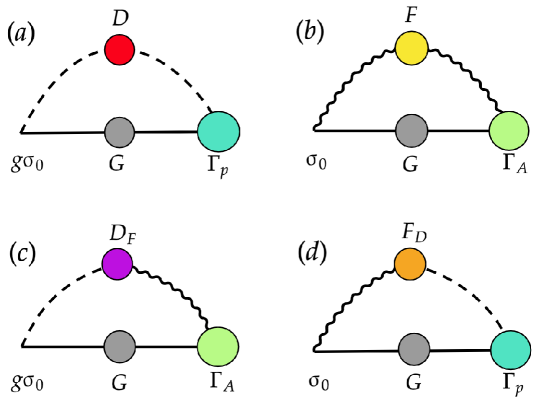
Figure 1: The four diagrams (a)-(d) correspond to the four terms of the fermion self-energy given by Eq. (27). Dashed (wavy) line represents the propagation of the boson $\phi$ ($A$).

According to Eq. (27), the fermion self-energy $\Sigma(p)=G^{-1}(p)-G_{0}^{-1}(p)$ consists of four terms. The corresponding diagrams are shown in Fig. 1. The first two terms originate from pure EPI and pure Coulomb interaction, respectively. The last two terms represent the contributions from the mixing of two bosons. In previous theoretical works, the last two terms are often naively neglected. In Eq. (27), there are four two-point correlation functions, namely $D(q)$, $F(q)$, $D_{F}(q)$, and $F_{D}(q)$, and two interaction vertex functions, including $\Gamma_{p}(q,p)$ and $\Gamma_{A}(q,p)$. These six functions are all unknown and each of them satisfies its own DS integral equation. According to the analysis presented in Refs. Liu21 ; Pan21 , the DS equations of $\Gamma_{p}(q,p)$ and $\Gamma_{A}(q,p)$ are extremely complicated since they are coupled to an infinite number of DS equations obeyed by all the higher-point correlation functions.

At first glance, the above DS equation of $G(p)$ is not self-closed and cannot be solved because it contains six unknown functions $D(q)$, $F(q)$, $D_{F}(q)$, $F_{D}(q)$, $\Gamma_{p}(q,p)$, and $\Gamma_{A}(q,p)$. Fortunately, we find that it is not necessary to determine each of these six functions separately. Indeed, these six functions satisfy two exact identities. The derivation of the exact identities is based on the invariance of partition function $Z$ under an arbitrary infinitesimal change of the scalar field $\phi$. Such an invariance gives rise to

$$\langle\mathbb{D}(x)\phi(x)-g\sum_{\sigma}^{N}\bar{\psi}_{\sigma}(x)\gamma_{0}\psi_{\sigma}(x)+J\rangle=0,$$ (28)

which is simply the mean value of the equation of the motion of phonons. Since $\langle\phi(x)\rangle=\frac{\delta W}{J(x)}$, we re-write this equation as

$$\mathbb{D}(x)\frac{\delta W}{J(x)}=g\sum_{\sigma}^{N}\langle\bar{\psi}_{\sigma}(x)\gamma_{0}\psi_{\sigma}(x)\rangle+J.$$ (29)

Then we carry out functional derivatives with respect to sources $\eta(z)$ and $\bar{\eta}(y)$ in order. After taking all sources to zero, we have

$$\mathbb{D}(x)\langle\phi(x)\psi(y)\bar{\psi}(z)\rangle_{c}=g\langle\sum_{\sigma}^{N}\bar{\psi}_{\sigma}(x)\gamma_{0}\psi_{\sigma}(x)\psi(y)\bar{\psi}(z)\rangle_{c},$$ (30)

where Eq. (15) is used in the calculation. In order to find out the consequence of this equation, we need to perform a Fourier transformation for both sides. With the help of Eq. (23), it is easy to find that the left-hand side (l.h.s.) of Eq. (30) becomes

$$D_{0}^{-1}(q)\Big{[}-D(q)G(p+q)\Gamma_{p}(q,p)G(p)-D_{F}(q)G(p+q)\Gamma_{A}(q,p)G(p)\Big{]}$$ (31)

after making Fourier transformation. The free phonon propagator $D_{0}(q)$ is obtained by Fourier transformation of the operator $\mathbb{D}(x)$. Then we turn to deal with the right hand side (r.h.s.) of Eq. (30). It can be verified that the Lagrangian density $\mathcal{L}$ given by Eq. (1) respects a U(1) symmetry $\psi\rightarrow e^{i\theta}\psi$, where $\theta$ is an infinitesimal constant. Noether theorem dictates that this symmetry leads to a conserved current $j_{\mu}\equiv\left(j_{0},j_{1},j_{2}\right)$, satisfying the identity

$$\sum_{\mu}\partial^{\mu}j_{\mu}(x)\equiv\partial_{0}j_{0}(x)-\partial_{1}j_{1}(x)-\partial_{2}j_{2}(x)=0.$$ (32)

The three components of local current operator $j_{\mu}(x)$ can be expressed in terms of spinor field as

$$j_{0}(x) = \sum_{\sigma}^{N}\bar{\psi}_{\sigma}(x)\gamma_{0}\psi_{\sigma}(x),$$ (33)

$$j_{1}(x) = \sum_{\sigma}^{N}\bar{\psi}_{\sigma}(x)\gamma_{1}\psi_{\sigma}(x),$$ (34)

$$j_{2}(x) = \sum_{\sigma}^{N}\bar{\psi}_{\sigma}(x)\gamma_{2}\psi_{\sigma}(x).$$ (35)

Now the r.h.s. of Eq. (30) is equivalent to $g\langle j_{0}(x)\psi(y)\bar{\psi}(z)\rangle$. Here it is convenient to introduce a special current vertex function $\Gamma_{0}(x-z,z-y)$ and define it via the relation

$$\langle\sum_{\sigma}^{N}\bar{\psi}_{\sigma}(x)\gamma_{0}\psi_{\sigma}(x)\psi(y)\bar{\psi}(z)\rangle_{c}=-\int d\xi d\xi^{\prime}G(y-\xi)\Gamma_{0}(\xi-x,x-\xi^{\prime})G(\xi^{\prime}-z).$$ (36)

The Fourier transformation of $\Gamma_{0}(\xi-x,x-\xi^{\prime})$ is given by

$$\Gamma_{0}(\xi-x,x-\xi^{\prime})=\int dqdpe^{-i(p+q)\cdot(\xi-x)-ip\cdot(x-\xi^{\prime})}\Gamma_{0}(q,p).$$ (37)

Fourier transforming the r.h.s. of Eq. (30) leads to

$$\int dxdye^{i(p+q)\cdot(y-x)}e^{ip\cdot(x-z)}g\langle\sum_{\sigma}^{N}\bar{\psi}_{\sigma}(x)\gamma_{0}\psi_{\sigma}(x)\psi(y)\bar{\psi}(z)\rangle_{c}\rightarrow-gG(p+q)\Gamma_{0}(q,p)G(p).$$ (38)

The two formulae shown in Eq. (31) and Eq. (38) must be equal, i.e.,

$$D_{0}^{-1}(q)\Big{[}D(q)G(p+q)\Gamma_{p}(q,p)G(p)+D_{F}(q)G(p+q)\Gamma_{A}(q,p)G(p)\Big{]}=gG(p+q)\Gamma_{0}(q,p)G(p),$$ (39)

which can be simplified to a more compact form

$$D(q)\Gamma_{p}(q,p)+D_{F}(q)\Gamma_{A}(q,p)=D_{0}(q)g\Gamma_{0}(q,p).$$ (40)

The above analysis can be easily applied to treat the coupling between $\psi$ and $A$. Repeating the same calculational steps gives rise to another important identity

$$F_{D}(q)\Gamma_{p}(q,p)+F(q)\Gamma_{A}(q,p)=F_{0}(q)\Gamma_{0}(q,p),$$ (41)

where $F_{0}(q)$ is the free propagator of $A$ boson, obtained by performing Fourier transformation to the operator $\mathbb{F}(x)$. In Fig. 2, we show a diagrammatic illustration of the two identities given by Eq. (40) and Eq. (41).

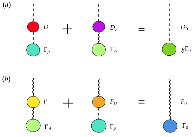
Figure 2: The Feynman diagrams plotted in (a) and (b) correspond to Eq. (40) and Eq. (41), respectively. The free propagators $D_{0}$ and $F_{0}$ are represented by dashes and wavy lines without carrying a shadowed circle, respectively.

Making use of the two identities of Eq. (40) and Eq. (41), the originally complicated DS equation (27) can be greatly simplified to

$$G^{-1}(p)=G_{0}^{-1}(p)-i\int dq\left[g^{2}D_{0}(q)+F_{0}(q)\right]\gamma_{0}G(p+q)\Gamma_{0}(q,p).$$ (42)

The sum of the four self-energy diagrams shown in Fig. 1 are now replaced with the sum of the two diagrams shown in Fig. 3. This equation looks much simpler, but is still hard to solve since the function $\Gamma_{0}(q,p)$ remains unknown. The equation of $G(p)$ could be entirely self-closed if and only if $\Gamma_{0}(q,p)$ depends solely on $G(p)$. Our next task is to find out the relationship between $\Gamma_{0}(q,p)$ and $G(p)$.

Figure 3: Diagrams for the fermion self-energy appearing in the simplified DS equation (42).

III Generalized Ward-Takahashi identities

In this section we will show that the function $\Gamma_{0}(q,p)$ can be expressed purely in terms of $G(p)$. The calculational procedure that leads to the exact relation between $\Gamma_{0}(q,p)$ and $G(p)$ has previously been illustrated with great details in Refs. Liu21 ; Pan21 . Here, in order to make this paper self-contained, we briefly outline the main calculational steps.

Now make the following global transformation to the spinor field $\psi(x)$:

$$\psi(x)\to e^{i\theta\gamma_{m}}\psi(x),\quad\bar{\psi}(x)\to\psi^{{\dagger}}(x)e^{-i\theta\gamma_{m}}\gamma_{0}.$$ (43)

Here, $\theta$ is an infinitesimal constant and $\gamma_{m}$ denotes a generic $4\times 4$ matrix. Generically, there are totally $32$ different choices for $\gamma_{m}$. $16$ of them are $\gamma_{m}=I$, $\gamma_{m}=\gamma_{0}$, $\gamma_{m}=\gamma_{1}$, $\gamma_{m}=\gamma_{2}$, $\gamma_{m}=\gamma_{3}$, $\gamma_{m}=\gamma_{0}\gamma_{1}\equiv\gamma_{01}$, $\gamma_{m}=\gamma_{0}\gamma_{2}\equiv\gamma_{02}$, $\gamma_{m}=\gamma_{0}\gamma_{3}\equiv\gamma_{03}$, $\gamma_{m}=\gamma_{1}\gamma_{2}\equiv\gamma_{12}$, $\gamma_{m}=\gamma_{1}\gamma_{3}\equiv\gamma_{13}$, $\gamma_{m}=\gamma_{2}\gamma_{3}\equiv\gamma_{23}$, $\gamma_{m}=\gamma_{0}\gamma_{1}\gamma_{2}\equiv\gamma_{012}$, $\gamma_{m}=\gamma_{0}\gamma_{1}\gamma_{3}\equiv\gamma_{013}$, $\gamma_{m}=\gamma_{0}\gamma_{2}\gamma_{3}\equiv\gamma_{023}$, $\gamma_{m}=\gamma_{1}\gamma_{2}\gamma_{3}\equiv\gamma_{123}$, and $\gamma_{m}=\gamma_{0}\gamma_{1}\gamma_{2}\gamma_{3}\equiv\gamma_{0123}$. The rest $16$ matrices are obtained by multiplying each of these matrices by $i$. It should be emphasized that we do not require the total Lagrangian density $\mathcal{L}_{T}$ defined by Eq. (7) to be invariant under the above global transformation. In fact, $\mathcal{L}_{T}$ is invariant under the transformation (43) only when $\gamma_{m}=I$. Different from $\mathcal{L}_{T}$, the partition function $Z[J,K,\bar{\eta},\eta]$ should be invariant under the transformation $\psi\to e^{i\theta\gamma_{m}}\psi$ for any choice of $\gamma_{m}$, since $Z[J,K,\bar{\eta},\eta]$ is obtained by integrating out all the possible configurations of $\psi$ and $\psi^{{\dagger}}$.

Below we will demonstrate that the invariance of $Z[J,K,\bar{\eta},\eta]$ under the infinitesimal transformation Eq. (43) imposes a stringent constraint on the relation between $\Gamma_{0}(q,p)$ and $G(p)$. Making use of this invariance, we derive the following equation

$$\langle\big{(}i\partial_{0}\bar{\psi}_{\sigma}(x)\gamma_{0}-i\partial_{1}\bar{\psi}_{\sigma}(x)\gamma_{1}-i\partial_{2}\bar{\psi}_{\sigma}(x)\gamma_{2}\big{)}\gamma_{m}\psi_{\sigma}(x)\rangle+\langle\psi_{\sigma}^{\dagger}(x)\gamma_{m}^{{\dagger}}\gamma_{0}\big{(}i\partial_{0}\gamma_{0}-i\partial_{1}\gamma_{1}-i\partial_{2}\gamma_{2}\big{)}\psi_{\sigma}(x)\rangle$$ (44)

$$= \bar{\eta}_{\sigma}(x)\gamma_{m}\langle\psi_{\sigma}(x)\rangle-\langle\psi_{\sigma}^{{\dagger}}(x)\rangle\gamma_{m}^{{\dagger}}\gamma_{0}\eta_{\sigma}(x)$$

$$-g\langle\phi(x)\psi_{\sigma}^{{\dagger}}(x)(\gamma_{0}\gamma_{0}\gamma_{m}-\gamma_{m}^{{\dagger}}\gamma_{0}\gamma_{0})\psi_{\sigma}(x)\rangle-\langle A(x)\psi_{\sigma}^{{\dagger}}(x)(\gamma_{0}\gamma_{0}\gamma_{m}-\gamma_{m}^{{\dagger}}\gamma_{0}\gamma_{0})\psi_{\sigma}(x)\rangle,$$

which comes from the identity $\delta Z=0$. Throughout this section, the repeated flavor index $\sigma$ needs to be summed over. But we omit the summation notation for simplicity. As the next step, we carry out functional derivatives $\frac{\delta^{2}}{\delta\bar{\eta}(y)\delta\eta(z)}|_{0}$ to both sides of Eq. (44) and obtain

$$\langle\big{(}i\partial_{0}\bar{\psi}_{\sigma}(x)\gamma_{0}-i\partial_{1}\bar{\psi}_{\sigma}(x)\gamma_{1}-i\partial_{2}\bar{\psi}_{\sigma}(x)\gamma_{2}\big{)}\gamma_{m}\psi_{\sigma}(x)\psi(y)\bar{\psi}(z)\rangle_{c}$$ (45)

$$+\langle\psi_{\sigma}^{{\dagger}}(x)\gamma_{m}^{{\dagger}}\gamma_{0}\big{(}i\partial_{0}\gamma_{0}-i\partial_{1}\gamma_{1}-i\partial_{2}\gamma_{2}\big{)}\psi_{\sigma}(x)\psi(y)\bar{\psi}(z)\rangle_{c}$$

$$= \delta(x-y)\gamma_{m}G(x-z)-G(y-x)\gamma_{0}\gamma_{m}^{{\dagger}}\gamma_{0}\delta(x-z)$$

$$-g\langle\phi(x)\psi_{\sigma}^{\dagger}(x)(\gamma_{0}\gamma_{0}\gamma_{m}-\gamma_{m}^{{\dagger}}\gamma_{0}\gamma_{0})\psi_{\sigma}(x)\psi(y)\bar{\psi}(z)\rangle_{c}$$

$$-\langle A(x)\psi_{\sigma}^{\dagger}(x)(\gamma_{0}\gamma_{0}\gamma_{m}-\gamma_{m}^{{\dagger}}\gamma_{0}\gamma_{0})\psi_{\sigma}(x)\psi(y)\bar{\psi}(z)\rangle_{c}.$$

While this formula is strictly valid, it is formally too complicated. In particular, the third term of the r.h.s. is a very special correlation function defined by the mean value of the product of five field operators. The forth term has a similar structure. The presence of such special correlation functions makes it difficult to extract useful information on the relation between $\Gamma_{0}(q,p)$ and $G(p)$. Fortunately, it is easy to see that these two five-point correlation functions can be eliminated if the matrix $\gamma_{m}$ is properly chosen to ensure that $\gamma_{0}\gamma_{0}\gamma_{m}-\gamma_{m}^{{\dagger}}\gamma_{0}\gamma_{0}=0$. Let us choose the following four matrices

$$\gamma_{m}=I,\quad\gamma_{m}=\gamma_{01},\quad\gamma_{m}=\gamma_{02},\quad\gamma_{m}=i\gamma_{12}.$$ (46)

Substituting them into Eq. (45) eliminates the third and the forth terms of the r.h.s. of this equation, leaving us with an identity of the form

$$\langle\big{(}i\partial_{0}\bar{\psi}_{\sigma}(x)\gamma_{0}-i\partial_{1}\bar{\psi}_{\sigma}(x)\gamma_{1}-i\partial_{2}\bar{\psi}_{\sigma}(x)\gamma_{2}\big{)}\gamma_{m}\psi_{\sigma}(x)\psi(y)\bar{\psi}(z)\rangle_{c}$$ (47)

$$+\langle\psi_{\sigma}^{{\dagger}}(x)\gamma_{m}^{{\dagger}}\gamma_{0}\big{(}i\partial_{0}\gamma_{0}-i\partial_{1}\gamma_{1}-i\partial_{2}\gamma_{2}\big{)}\psi_{\sigma}(x)\psi(y)\bar{\psi}(z)\rangle_{c}$$

$$= \delta(x-y)\gamma_{m}G(x-z)-G(y-x)\gamma_{0}\gamma_{m}^{{\dagger}}\gamma_{0}\delta(x-z).$$

For $\gamma_{m}=I$, the identity of Eq. (47) becomes

$$\langle\big{(}i\partial_{0}\bar{\psi}_{\sigma}(x)\gamma_{0}-i\partial_{1}\bar{\psi}_{\sigma}(x)\gamma_{1}-i\partial_{2}\bar{\psi}_{\sigma}(x)\gamma_{2}\big{)}\psi_{\sigma}(x)\psi(y)\bar{\psi}(z)\rangle_{c}$$ (48)

$$+\langle\bar{\psi}_{\sigma}(x)\big{(}i\partial_{0}\gamma_{0}-i\partial_{1}\gamma_{1}-i\partial_{2}\gamma_{2}\big{)}\psi_{\sigma}(x)\psi(y)\bar{\psi}(z)\rangle_{c}$$

$$= \delta(x-y)IG(x-z)-G(y-x)I\delta(x-z).$$

Using the conserved current operator $j_{\mu}(x)$ define by Eqs. (33-35), we find that Eq. (48) can be re-written as

$$i\partial^{\mu}\langle j_{\mu}(x)\psi(y)\bar{\psi}(z)\rangle_{c} \equiv i\partial_{0}\langle j_{0}(x)\psi(y)\bar{\psi}(z)\rangle_{c}-i\partial_{1}\langle j_{1}(x)\psi(y)\bar{\psi}(z)\rangle_{c}-i\partial_{2}\langle j_{2}(x)\psi(y)\bar{\psi}(z)\rangle_{c}$$ (49)

$$= \delta(x-y)G(x-z)-G(x-y)\delta(x-z).$$

The three correlation functions appearing in the l.h.s. of this equation are used to define three current vertex functions $\Gamma_{0,1,2}$ as follows

$$\langle j_{0,1,2}(x)\psi(y)\bar{\psi}(z)\rangle_{c}=-\int d\xi d\xi^{\prime}G(y-\xi)\Gamma_{0,1,2}(\xi-x,x-\xi^{\prime})G(\xi^{\prime}-z).$$ (50)

The function $\Gamma_{0}$ has already been encountered in in Sec. II, and its Fourier transformation is given by Eq. (37). The other two functions $\Gamma_{1}$ and $\Gamma_{2}$ can be transformed similarly, namely

$$\Gamma_{1,2}(\xi-x,x-\xi^{\prime})=\int dqdpe^{-i(p+q)\cdot(\xi-x)-ip\cdot(x-\xi^{\prime})}\Gamma_{1,2}(q,p).$$ (51)

The next step would be to substitute Eq. (50) into Eq. (49) and carry out Fourier transformation to both sides of Eq. (49). The calculation is straightforward. For instance, $i\partial_{0}\langle j_{1}(x)\psi(y)\bar{\psi}(z)\rangle_{c}$ can be Fourier transformed as follows

$$i\partial_{0}\langle j_{1}(x)\psi(y)\bar{\psi}(z)\rangle_{c}$$ (52)

$$= -i\partial_{0}\int d\xi d\xi^{\prime}G(y-\xi)\Gamma_{0}(\xi-x,x-\xi^{\prime})G(\xi^{\prime}-z)$$

$$= -i\partial_{0}\int d\xi d\xi^{\prime}\int dpdqdp^{\prime}dq^{\prime}e^{-i(p+q)\cdot(y-\xi)}G(p+q)e^{-i(p^{\prime}+q^{\prime})\cdot(\xi-x)-ip^{\prime}\cdot(x-\xi^{\prime})}\Gamma_{0}(q^{\prime},p^{\prime})e^{-ip\cdot(\xi^{\prime}-z)}G(p)$$

$$= -i\partial_{0}\int dpdqdp^{\prime}dq^{\prime}e^{-i(p+q)\cdot y}G(p+q)\delta\big{(}p+q-(p^{\prime}+q^{\prime})\big{)}e^{i(p^{\prime}+q^{\prime})\cdot x-ip^{\prime}\cdot x}\Gamma_{0}(q^{\prime},p^{\prime})\delta(p^{\prime}-p)e^{ip\cdot z}G(p)$$

$$= -i\partial_{0}\int dpdqe^{-i(p+q)\cdot(y-x)}e^{-ip\cdot(x-z)}G(p+q)\Gamma_{0}(q,p)G(p)$$

$$= \int dpdqe^{-i(p+q)\cdot(y-x)}e^{-ip\cdot(x-z)}q_{0}G(p+q)\Gamma_{0}(q,p)G(p).$$

After completing all the analytical calculations, we eventually convert Eq. (49) into

$$G(p+q)\big{[}q_{0}\Gamma_{0}(q,p)-q_{1}\Gamma_{1}(q,p)-q_{2}\Gamma_{2}(q,p)\big{]}G(p)=G(p)-G(p+q),$$ (53)

which can be further simplified to

$$q_{0}\Gamma_{0}(q,p)-q_{1}\Gamma_{1}(q,p)-q_{2}\Gamma_{2}(q,p)=G^{-1}(p+q)-G^{-1}(p).$$ (54)

Recall this identity is derived by making the transformation $\psi\to e^{i\theta}\psi$ and $\bar{\psi}\to e^{-i\theta}\bar{\psi}$, which is nothing but the global U(1) symmetry of the Lagrangian density. Thus this identity is indeed the ordinary WTI induced by the conservation of particle number.

As demonstrated at the end of Sec. II, the DS equation of the full fermion propagator $G(p)$, given by Eq. (42), would be made entirely self-closed if we could express the function $\Gamma_{0}(q,p)$ purely in terms of $G(p)$. Apparently, it is not possible to entirely determine $\Gamma_{0}(q,p)$ by solving the above WTI, since $\Gamma_{1}(q,p)$ and $\Gamma_{2}(q,p)$ are also unknown. To determine $\Gamma_{0}(q,p)$, we need to find our more identities satisfied by $\Gamma_{0}(q,p)$, $\Gamma_{1}(q,p)$, $\Gamma_{2}(q,p)$, and $G(p)$.

Next we choose $\gamma_{m}=\gamma_{01}$ and use this matrix to express the identity of Eq. (47) in the form

$$\langle\big{(}i\partial_{0}\bar{\psi}_{\sigma}(x)\gamma_{1}-i\partial_{1}\bar{\psi}_{\sigma}(x)\gamma_{0}-i\partial_{2}\bar{\psi}_{\sigma}(x)\gamma_{0}\gamma_{1}\gamma_{2}\big{)}\psi_{\sigma}(x)\psi(y)\bar{\psi}(z)\rangle_{c}$$ (55)

$$+\langle\bar{\psi}_{\sigma}(x)\big{(}i\partial_{0}\gamma_{1}-i\partial_{1}\gamma_{0}-i\partial_{2}\gamma_{0}\gamma_{1}\gamma_{2}\big{)}\psi_{\sigma}(x)\psi(y)\bar{\psi}(z)\rangle_{c}$$

$$= \delta(x-y)\gamma_{0}\gamma_{1}G(x-z)+G(y-x)\gamma_{0}\gamma_{1}\delta(x-z).$$

Apart from the current operators $j_{0}(x)$ and $j_{1}(x)$, here we need to define one more current operator

$$j_{012}(x)=\bar{\psi}_{\sigma}(x)\gamma_{012}\psi_{\sigma}(x),$$ (56)

where $\gamma_{012}=\gamma_{0}\gamma_{1}\gamma_{2}$. This new current operator also corresponds to a new current vertex function $\Gamma_{012}$, which is defined as

$$\langle j_{012}(x)\psi(y)\bar{\psi}(z)\rangle_{c} = -\int d\xi d\xi^{\prime}G(y-\xi)\Gamma_{012}(\xi-x,x-\xi^{\prime})G(\xi^{\prime}-z),$$ (57)

$$\Gamma_{012}(\xi-x,x-\xi^{\prime}) = \int dqdpe^{-i(p+q)\cdot(\xi-x)-ip\cdot(x-\xi^{\prime})}\Gamma_{012}(q,p)..$$ (58)

The l.h.s. of Eq. (55) is a little more complicated than that of Eq. (48). Originally, the bilinear operators $j_{0}(x)$, $j_{1}(x)$, $j_{2}(x)$, and $j_{012}(x)$ are defined as products of $\psi(x)$ and $\bar{\psi}(x)$, which are supposed to be located at the same time-space point $x$. In order to express the l.h.s. of Eq. (55) in terms of $j_{012}(x)$, we need to move the partial derivative operator $\partial_{2}$ out of the mean value. This can be achieved by employing the point-splitting technique that is widely applied to regularize the short-distance singularity caused by the locality of bilinear current operators in high-energy physics Dirac ; Schwinger ; Jackiw ; Takahashi78 ; Peskin ; Schnabl . Using this technique Takahashi78 ; He01 , one could re-define current operators at two very close but distinct points $x$ and $x^{\prime}$, namely

$$j_{0,1,2,012}(x,x^{\prime})=\bar{\psi}_{\sigma}(x^{\prime})\gamma_{0,1,2,012}\psi_{\sigma}(x).$$ (59)

The limit $x\rightarrow x^{\prime}$ should be taken after all calculations are completed. Now Eq. (55) becomes

$$i\partial_{0}\langle j_{1}(x)\psi(y)\bar{\psi}(z)\rangle_{c}-i\partial_{1}\langle j_{0}(x)\psi(y)\bar{\psi}(z)\rangle_{c}-\lim_{x^{\prime}\to x}(i\partial_{2^{\prime}}-i\partial_{2})\langle j_{012}(x,x^{\prime})\psi(y)\bar{\psi}(z)\rangle_{c}$$ (60)

$$= \delta(x-y)\gamma_{0}\gamma_{1}G(x-z)+G(y-x)\gamma_{0}\gamma_{1}\delta(x-z).$$

Inserting Eq. (50) and Eq. (57) into Eq. (60) makes it possible to use $\Gamma_{1}$, $\Gamma_{0}$, and $\Gamma_{012}$ to express the three terms of l.h.s. of this equation, respectively. The first two terms can be Fourier transformed in exactly the same way as Eq. (52). The third term is computed as

$$\lim_{x^{\prime}\to x}(i\partial_{2^{\prime}}-i\partial_{2})\langle j_{012}(x,x^{\prime})\psi(y)\bar{\psi}(z)\rangle_{c}$$ (61)

$$= -\lim_{x^{\prime}\to x}(i\partial_{2^{\prime}}-i\partial_{2})\int d\xi d\xi^{\prime}G(y-\xi)\Gamma_{012}(\xi-x^{\prime},x-\xi^{\prime})G(\xi^{\prime}-z)$$

$$= -\lim_{x^{\prime}\to x}(i\partial_{2^{\prime}}-i\partial_{2})\int d\xi d\xi^{\prime}\int dpdqdp^{\prime}dq^{\prime}e^{-i(p+q)\cdot(y-\xi)}G(p+q)$$

$$\times e^{-i(p^{\prime}+q^{\prime})\cdot(\xi-x^{\prime})-ip^{\prime}\cdot(x-\xi^{\prime})}\Gamma_{012}(q^{\prime},p^{\prime})e^{-ip\cdot(\xi^{\prime}-z)}G(p)$$

$$= -\lim_{x^{\prime}\to x}(i\partial_{2^{\prime}}-i\partial_{2})\int dpdqdp^{\prime}dq^{\prime}e^{-i(p+q)\cdot y}G(p+q)\delta\big{(}p+q-(p^{\prime}+q^{\prime})\big{)}$$

$$\times e^{i(p^{\prime}+q^{\prime})\cdot x^{\prime}-ip^{\prime}\cdot x}\Gamma_{012}(q^{\prime},p^{\prime})\delta(p^{\prime}-p)e^{ip\cdot z}G(p)$$

$$= -\lim_{x^{\prime}\to x}(i\partial_{2^{\prime}}-i\partial_{2})\int dpdqe^{-i(p+q)\cdot(y-x^{\prime})}e^{-ip\cdot(x-z)}G(p+q)\Gamma_{012}(q,p)G(p)$$

$$= \lim_{x^{\prime}\to x}\int dpdq(p_{2}+q_{2}+p_{2})e^{-i(p+q)\cdot(y-x^{\prime})}e^{-ip\cdot(x-z)}G(p+q)\Gamma_{012}(q,p)G(p)$$

$$= \int dpdqe^{-i(p+q)\cdot(y-x)}e^{-ip\cdot(x-z)}(2p_{2}+q_{2})G(p+q)\Gamma_{012}(q,p)G(p).$$

Finally, we obtain from Eq. (60) the following identity

$$q_{0}\Gamma_{1}(q,p)-q_{1}\Gamma_{0}(q,p)-(2p_{2}+q_{2})\Gamma_{012}(q,p)=-G^{-1}(p+q)\gamma_{01}-\gamma_{01}G^{-1}(p).$$ (62)

This identity has an analogous form to the ordinary WTI given by Eq. (54). There is an important different between them. The ordinary WTI is induced by the U(1)-symmetry of the Lagrangian density. In contrast, the identity given by Eq. (62) originates from the invariance of the partition function under the transformation $\psi\rightarrow e^{i\theta\gamma_{01}}\psi$, which is not a symmetry of the model as it apparently changes the Lagrangian density.

Thus far, we have derived two identities obeyed by four different current vertex functions $\Gamma_{0}(q,p)$, $\Gamma_{1}(q,p)$, $\Gamma_{2}(q,p)$, and $\Gamma_{012}(q,p)$. We still need at least two more identities to completely determine each of these functions. For $\gamma_{m}=\gamma_{02}$, the identity of Eq. (47) becomes

$$\langle\big{(}i\partial_{0}\bar{\psi}_{\sigma}\gamma_{2}+i\partial_{1}\bar{\psi}_{\sigma}\gamma_{0}\gamma_{1}\gamma_{2}-i\partial_{2}\bar{\psi}_{\sigma}\gamma_{0}\big{)}\psi_{\sigma}\psi(y)\bar{\psi}(z)\rangle_{c}$$ (63)

$$+\langle\bar{\psi}_{\sigma}\big{(}i\partial_{0}\gamma_{2}-i\partial_{1}\gamma_{0}\gamma_{1}\gamma_{2}-i\partial_{2}\gamma_{0}\big{)}\psi_{\sigma}\psi(y)\bar{\psi}(z)\rangle_{c}$$

$$= \delta(x-y)\gamma_{0}\gamma_{2}G(x-z)+G(y-x)\gamma_{0}\gamma_{2}\delta(x-z).$$

Applying point-splitting trick to this equation gives rise to

$$i\partial_{0}\langle j_{2}(x)\psi(y)\bar{\psi}(z)\rangle_{c}+\lim_{x^{\prime}\to x}(i\partial_{1^{\prime}}-i\partial_{1})\langle j_{012}(x,x^{\prime})\psi(y)\bar{\psi}(z)\rangle_{c}-i\partial_{2}\langle j_{0}(x)\psi(y)\bar{\psi}(z)\rangle_{c}$$ (64)

$$= \delta(x-y)\gamma_{0}\gamma_{2}G(x-z)+G(y-x)\gamma_{0}\gamma_{2}\delta(x-z).$$

Finally, choosing $\gamma_{m}=i\gamma_{12}$ makes Eq. (47) to become

$$\langle\big{(}i\partial_{0}\bar{\psi}_{\sigma}i\gamma_{0}\gamma_{1}\gamma_{2}+i\partial_{1}\bar{\psi}_{\sigma}i\gamma_{2}-i\partial_{2}\bar{\psi}_{\sigma}i\gamma_{1}\big{)}\psi_{\sigma}\psi(y)\bar{\psi}(z)\rangle_{c}$$ (65)

$$+\langle\bar{\psi}_{\sigma}\big{(}i\partial_{0}i\gamma_{0}\gamma_{1}\gamma_{2}-i\partial_{1}i\gamma_{2}-i\partial_{2}(-i\gamma_{1})\big{)}\psi_{\sigma}\psi(y)\bar{\psi}(z)\rangle_{c}$$

$$= \delta(x-y)i\gamma_{1}\gamma_{2}G(x-z)-G(y-x)i\gamma_{1}\gamma_{2}\delta(x-z),$$

which can be re-written as

$$i\partial_{0}\langle j_{012}(x)\psi(y)\bar{\psi}(z)\rangle_{c}+\lim_{x^{\prime}\to x}(i\partial_{1^{\prime}}-i\partial_{1})\langle j_{2}(x,x^{\prime})\psi(y)\bar{\psi}(z)\rangle_{c}$$ (66)

$$-\lim_{x^{\prime}\to x}(i\partial_{2^{\prime}}-i\partial_{2})\langle j_{1}(x,x^{\prime})\psi(y)\bar{\psi}(z)\rangle_{c}$$

$$= \delta(x-y)\gamma_{1}\gamma_{2}G(x-z)-G(y-x)\gamma_{1}\gamma_{2}\delta(x-z).$$

After performing Fourier transformations, we find that Eq. (64) and Eq. (66) yield two identities:

$$q_{0}\Gamma_{2}(q,p)-q_{2}\Gamma_{0}(q,p)+(2p_{1}+q_{1})\Gamma_{012}(q,p) = -G^{-1}(p+q)\gamma_{02}-\gamma_{02}G^{-1}(p),$$ (67)

$$q_{0}\Gamma_{012}(q,p)-(2p_{2}+q_{2})\Gamma_{1}(q,p)+(2p_{1}+q_{1})\Gamma_{2}(q,p) = G^{-1}(p+q)\gamma_{12}-\gamma_{12}G^{-1}(p).$$ (68)

The four independent identities given by Eq. (54), Eq. (62), Eq. (67), and Eq. (68) are generated respectively by making the following four infinitesimal transformations of the spinor field:

$$\psi\to e^{i\theta}\psi,\quad\psi\to e^{i\theta\gamma_{01}}\psi,\quad\psi\to e^{i\theta\gamma_{02}}\psi,\quad\psi\to e^{-\theta\gamma_{12}}\psi.$$

Among these transformations, the first one keeps the Lagrangian density intact and thus Eq. (54) is a genuine symmetry-induced WTI. The rest three transformations are clearly not symmetries of the model. The forth one is not even a unitary transformation. Therefore, the last three identities are different from Eq. (54). Nevertheless, we would regard all of the four identities as generalized WTIs for two reasons. First, they have very similar forms. Second, they can be derived in a unified way from the invariance of the partition function.

These four generalized WTIs can be expressed in the following compact form:

$$M\begin{pmatrix}\Gamma_{0}(q,p)\\ \Gamma_{1}(q,p)\\ \Gamma_{2}(q,p)\\ \Gamma_{012}(q,p)\end{pmatrix}=\begin{pmatrix}G^{-1}(p+q)-G^{-1}(p)\\ -G^{-1}(p+q)\gamma_{01}-\gamma_{01}G^{-1}(p)\\ -G^{-1}(p+q)\gamma_{02}-\gamma_{02}G^{-1}(p)\\ G^{-1}(p+q)\gamma_{12}-\gamma_{12}G^{-1}(p)\end{pmatrix}.$$ (69)

Here the matrix $M$ is given by

$$M=\begin{pmatrix}q_{0}&-q_{1}&-q_{2}&0\\ -q_{1}&q_{0}&0&-(2p_{2}+q_{2})\\ -q_{2}&0&q_{0}&+(2p_{1}+q_{1})\\ 0&-(2p_{2}+q_{2})&(2p_{1}+q_{1})&q_{0}\end{pmatrix}.$$ (70)

Now each of the four unknown functions $\Gamma_{0}(q,p)$, $\Gamma_{1}(q,p)$, $\Gamma_{2}(q,p)$, and $\Gamma_{012}(q,p)$ can be determined by solving the four coupled identities shown in Eq. (69). According to Eq. (42), we only need to know $\Gamma_{0}(q,p)$. From Eq. (69), it is easy to obtain

$$\Gamma_{0}(q,p) = \frac{1}{|M|}\Big{[}|M_{11}|\left(G^{-1}(p+q)\gamma_{0}-\gamma_{0}G^{-1}(p)\right)-|M_{21}|\left(-G^{-1}(p+q)\gamma_{01}-\gamma_{01}G^{-1}(p)\right)$$ (71)

$$+|M_{31}|\left(-G^{-1}(p+q)\gamma_{02}-\gamma_{02}G^{-1}(p)\right)-|M_{41}|\left(G^{-1}(p+q)\gamma_{012}-\gamma_{012}G^{-1}(p)\right)\Big{]},$$

where

$$|M| = q_{0}^{2}\left(q_{0}^{2}-q_{1}^{2}-q_{2}^{2}-(2p_{1}+q_{1})^{2}-(2p_{2}+q_{2})^{2}\right)+\big{(}q_{1}(2p_{1}+q_{1})+q_{2}(2p_{2}+q_{2})\big{)}^{2},$$

$$|M_{11}| = q_{0}\left(q_{0}^{2}-(2p_{1}+q_{1})^{2}-(2p_{2}+q_{2})^{2}\right),$$

$$|M_{21}| = q_{1}(2p_{1}+q_{1})^{2}-q_{1}q_{0}^{2}+q_{2}(2p_{1}+q_{1})(2p_{2}+q_{2}),$$

$$|M_{31}| = q_{2}q_{0}^{2}-q_{2}(2p_{2}+q_{2})^{2}-q_{1}(2p_{1}+q_{1})(2p_{2}+q_{2}),$$

$$|M_{41}| = q_{0}q_{1}(2p_{2}+q_{2})-q_{0}q_{2}(2p_{1}+q_{1}).$$ (72)

Since $\Gamma_{0}(q,p)$ depends only on the full fermion propagator $G(p)$, the DS equation of $G(p)$ given by Eq. (42) becomes completely self-closed and can be solved by the iteration method Liu21 . In passing, we have already confirmed that $\Gamma_{0}(q,p)$ does not exhibit any singularity since the zeroes of the denominator and numerator cancel each other out.

IV Numerical results of renormalized velocity

In this section, we discuss the physical implications of the numerical results of Eq. (42). It appears to be more convenient to perform numerical calculations if the Matsubara formalism of finite-temperature field theory is adopted. The real time $t$ appearing in the DS equation of fermion propagator should be replaced with the Matsubara time $\tau$, where $\tau\in[-T,T]$. The fermion momentum $p=(p_{0},\mathbf{p})$ becomes $p=(i\epsilon_{n},\mathbf{p})$, where $i\epsilon_{n}=i(2n+1)\pi T$, and the boson momentum $q=(q_{0},\mathbf{q})$ becomes $q=(i\omega_{n^{\prime}},\mathbf{q})$, where $i\omega_{n^{\prime}}=i2n^{\prime}\pi T$. $n$ and $n^{\prime}$ take all the integers.

As shown by Eq. (42), the DS equation of $G(p)$ contains the free propagators of two bosons. The free phonon propagator is

$$D_{0}(q)=\frac{2\Omega_{\mathbf{q}}}{(i\omega_{n^{\prime}})^{2}-\Omega_{\mathbf{q}}^{2}},$$ (73)

where the phonon dispersion is $\Omega_{\mathbf{q}}=c_{s}|\mathbf{q}|$ with $c_{s}$ being the phonon velocity Roy14 . The EPI strength parameter $g$ is a function of phonon momentum and formally defined Roy14 as

$$g\equiv g(q)=\sqrt{\lambda q/c_{s}},$$ (74)

where $q=|\mathbf{q}|$ is phonon momentum and $\lambda$ is a dimensionless tuning parameter. The precise value of $\lambda$ in undoped graphene is material dependent and should be determined by performing careful first-principle calculations. Here we regard $\lambda$ as a freely varying parameter and make a generic (material-independent) analysis. The free propagator of $A$ boson is

$$F_{0}(q)=\frac{2\pi\alpha}{|\mathbf{q}|},$$ (75)

which has the same form as the bare Coulomb interaction function. The fine structure constant

$$\alpha=\frac{e^{2}}{v_{F}\varepsilon},$$ (76)

characterizes the effective strength of Coulomb interaction Castroneto09 ; Sarma11 ; Kotov12 . It is well-known that $\alpha=0.8$ for graphene on SiO₂ substrate and $\alpha=2.2$ for graphene suspended in vacuum.

After incorporating the corrections induced by interactions, the free boson propagators will become dressed. The renormalization of such model parameters as $c_{s}$ and $\varepsilon$ can be studied by comparing the dressed boson propagators with the free boson propagators. In the literature (see Ref. Kotov12 for a review), the dressed boson propagators are usually calculated by employing the random phase approximation (RPA). In undoped graphene, the RPA-level, one-loop polarization function is found Son07 ; Kotov12 to have the form $\Pi_{\mathrm{RPA}}(q)=-\frac{N}{8}\frac{\mathbf{q}^{2}}{\sqrt{q_{0}^{2}+v^{2}\mathbf{q}^{2}}}$. Then the dressed phonon propagator is $D_{\mathrm{RPA}}(q)=\frac{1}{D_{0}^{-1}(q)+\Pi_{\mathrm{RPA}}(q)}$ and the dressed $A$ boson propagator (i.e., renormalized Coulomb interaction) is $F_{\mathrm{RPA}}(q)=\frac{1}{F_{0}^{-1}(q)+\Pi_{\mathrm{RPA}}(q)}$. Now both $D_{\mathrm{RPA}}(q)$ and $D_{\mathrm{RPA}}(q)$ are proportional to $\sim 1/N$. This provides a basis to classify all the Feynman diagrams according to the powers of $1/N$. The $1/N$ expansion has been adopted to investigate the physical effects of the Coulomb interaction in both perturbative calculations Son07 ; Son08 ; Hofmann14 ; Kotov12 and non-perturbative DS equation studies Khveshchenko01 ; Gorbar02 ; Khveshchenko04 ; Khveshchenko09 ; Liu09 ; Gamayun10 ; WangLiu12 ; WangLiu14 . However, $1/N$ expansion is well justified only in the $N\rightarrow\infty$ limit. Given that the physical flavor is rather small ($N=2$), the validity of $1/N$ expansion is in doubt.

Using our approach, the DS equations of fermion and boson propagators are decoupled Liu21 ; Pan21 . Thus the renormalization of boson propagators should be treated in a very different way from previous perturbative and non-perturbative calculations. Notice that the DS equation of full fermion propagator $G(p)$, given by Eq. (42), depends on the free boson propagators $D_{0}(q)$ and $F_{0}(q)$, rather than the dressed boson propagators $D(q)$ and $F(q)$. The interaction effects on the bosons are already indirectly embodied in the current vertex function $\Gamma_{0}(q,p)$. There would be an incorrect double counting if the dressed boson propagators $D(q)$ and $F(q)$ are substituted into Eq. (42). Therefore, the parameters $c_{s}$ and $\varepsilon$ appearing in $D_{0}(q)$ and $F_{0}(q)$ should take their bare values and must not be renormalized. For similar reasons, we need to use the bare value of EPI strength parameter $g$, whose renormalization is already taken into account by the function $\Gamma_{0}(q,p)$. The electric charge $e$ is also not renormalized Ye98 ; Herbut06 ; Pan21 . Different from the above parameters, the fermion velocity $v_{F}$ is renormalized by interactions. Below we demonstrate how to obtain the renormalized fermion velocity based on the solutions of $G(p)$.

The free fermion propagator is

$$G_{0}(p)=\frac{1}{i\epsilon_{n}\gamma_{0}-\mathbf{\gamma}\cdot\mathbf{p}}=-\frac{i\epsilon_{n}\gamma_{0}+\mathbf{\gamma}\cdot\mathbf{p}}{\epsilon_{n}^{2}+\mathbf{p}^{2}}.$$ (77)

Incorporating the interaction effects turns this free propagator into a full propagator that can be expressed as

$$G(p)=\frac{1}{A_{0}(\epsilon_{n},\mathbf{p})i\epsilon_{n}\gamma_{0}-A_{1}(\epsilon_{n},\mathbf{p})\mathbf{\gamma}\cdot\mathbf{p}}=-\frac{A_{0}(\epsilon_{n},\mathbf{p})i\epsilon_{n}\gamma_{0}+A_{1}(\epsilon_{n},\mathbf{p})\mathbf{\gamma}\cdot\mathbf{p}}{A_{0}^{2}(\epsilon_{n},\mathbf{p})\epsilon_{n}^{2}+A_{1}^{2}(\epsilon_{n},\mathbf{p})\mathbf{p}^{2}}.$$ (78)

The interactions effects are embodied in the two renormalization functions $A_{0}(\epsilon_{n},\mathbf{p})$ and $A_{1}(\epsilon_{n},\mathbf{p})$. Inserting $D_{0}(q)$, $F_{0}(q)$, $G_{0}(p)$, and $G(p)$ together with the function $\Gamma_{0}(q,p)$ given by Eq. (71) into Eq. (42) yields two self-consistent integral equations of $A_{0}(\epsilon_{n},\mathbf{p})$ and $A_{1}(\epsilon_{n},\mathbf{p})$.

For readers’ convenience, below we list all the formulae needed to express the self-closed DS equation of the full fermion propagator:

$$G^{-1}(\epsilon_{n},\mathbf{p}) = i\epsilon_{n}\gamma_{0}-\mathbf{\gamma\cdot p}+T\sum_{n^{\prime}}\int\frac{d^{2}\mathbf{q}}{(2\pi)^{2}}\left[g^{2}D_{0}(q)+F_{0}(q)\right]G(p+q)\Gamma_{0}(q,p),$$ (79)

$$\Gamma_{0}(q,p) = \frac{1}{|M|}\Big{[}|M_{11}|\left(G^{-1}(p+q)\gamma_{0}-\gamma_{0}G^{-1}(p)\right)-|M_{21}|\left(-G^{-1}(p+q)\gamma_{01}-\gamma_{01}G^{-1}(p)\right)$$ (80)

$$+|M_{31}|\left(-G^{-1}(p+q)\gamma_{02}-\gamma_{02}G^{-1}(p)\right)-|M_{41}|\left(G^{-1}(p+q)\gamma_{012}-\gamma_{012}G^{-1}(p)\right)\Big{]},$$

$$|M| = \omega_{n^{\prime}}^{2}\left(\omega_{n^{\prime}}^{2}+q_{1}^{2}+q_{2}^{2}+(2p_{1}+q_{1})^{2}+(2p_{2}+q_{2})^{2}\right)$$ (81)

$$+\big{(}q_{1}(2p_{1}+q_{1})+q_{2}(2p_{2}+q_{2})\big{)}^{2},$$

$$|M_{11}| = -i\omega_{n^{\prime}}\left(\omega_{n^{\prime}}^{2}+(2p_{1}+q_{1})^{2}+(2p_{2}+q_{2})^{2}\right),$$ (82)

$$|M_{21}| = q_{1}\left(\omega_{n^{\prime}}^{2}+(2p_{1}+q_{1})^{2}\right)+q_{2}(2p_{1}+q_{1})(2p_{2}+q_{2}),$$ (83)

$$|M_{31}| = -q_{2}\left(\omega_{n^{\prime}}^{2}+(2p_{2}+q_{2})^{2}\right)-q_{1}(2p_{1}+q_{1})(2p_{2}+q_{2}),$$ (84)

$$|M_{41}| = -i\omega_{n^{\prime}}q_{2}(2p_{1}+q_{1})+i\omega_{n^{\prime}}q_{1}(2p_{2}+q_{2}).$$ (85)

To facilitate numerical computations, we re-write these equations in the polar coordinate. We select $\mathbf{p}$ as the polar axis and define a new momentum $k=p+q$. Then $k_{1}=|\mathbf{k}|\cos\theta$, $k_{2}=|\mathbf{k}|\sin\theta$, $p_{1}=|\mathbf{p}|$, and $p_{2}=0$. Then Eqs. (81-85) become

$$|M| = \omega_{n^{\prime}}^{2}\left(\omega_{n^{\prime}}^{2}+2|\mathbf{k}|^{2}+2|\mathbf{p}|^{2}\right)+\left(|\mathbf{k}|^{2}-|\mathbf{p}|^{2}\right)^{2},$$ (86)

$$|M_{11}| = -i\omega_{n^{\prime}}\left(\omega_{n^{\prime}}^{2}+|\mathbf{k}|^{2}+|\mathbf{p}|^{2}+2|\mathbf{k}||\mathbf{p}|\cos\theta\right),$$ (87)

$$|M_{21}| = -\left(\omega_{n^{\prime}}^{2}+|\mathbf{p}|^{2}-|\mathbf{k}|^{2}\right)|\mathbf{p}|+\left(\omega_{n^{\prime}}^{2}+|\mathbf{k}|^{2}-|\mathbf{p}|^{2}\right)|\mathbf{k}|\cos\theta,$$ (88)

$$|M_{31}| = -|\mathbf{k}|\sin\theta\left(\omega_{n^{\prime}}^{2}+|\mathbf{k}|^{2}-|\mathbf{p}|^{2}\right),$$ (89)

$$|M_{41}| = -i2\omega_{n^{\prime}}|\mathbf{k}|\sin\theta|\mathbf{p}|.$$ (90)

The self-consistent integral equations of $A_{0}(p)$ and $A_{1}(p)$ are given by

$$A_{0}(p)\epsilon_{n} = \epsilon_{n}+T\sum_{n^{\prime}}\int\frac{|\mathbf{k}|d|\mathbf{k}|}{2\pi}\frac{1}{A_{0}^{2}(k)\epsilon_{n^{\prime}+n}^{2}+A_{1}^{2}(k)|\mathbf{k}|^{2}}$$ (91)

$$\times\Big{[}A_{0}(k)\epsilon_{n^{\prime}+n}\Big{(}f_{0kp1}\big{(}A_{0}(k)\epsilon_{n^{\prime}+n}-A_{0}(p)\epsilon_{n}\big{)}+f_{k0p1}A_{1}(k)|\mathbf{k}|-f_{k1p0}A_{1}(p)|\mathbf{p}|\Big{)}$$

$$+A_{1}(k)|\mathbf{k}|\Big{(}-f_{k0p1}\big{(}A_{0}(k)\epsilon_{n^{\prime}+n}-A_{0}(p)\epsilon_{n}\big{)}+f_{0kp1}A_{1}(k)|\mathbf{k}|-f_{1kp0}A_{1}(p)|\mathbf{p}|\Big{)}\Big{]},$$

$$A_{1}(p)|\mathbf{p}| = |\mathbf{p}|-T\sum_{n^{\prime}}\int\frac{|\mathbf{k}|d|\mathbf{k}|}{2\pi}\frac{1}{A_{0}^{2}(k)\epsilon_{n^{\prime}+n}^{2}+A_{1}^{2}(k)|\mathbf{k}|^{2}}$$ (92)

$$\times\Big{[}A_{0}(k)\epsilon_{n^{\prime}+n}\Big{(}f_{k1p0}\big{(}A_{0}(k)\epsilon_{n^{\prime}+n}-A_{0}(p)\epsilon_{n}\big{)}-f_{1kp0}A_{1}(k)|\mathbf{k}|+f_{0kp1}A_{1}(p)|\mathbf{p}|\Big{)}$$

$$+A_{1}(k)|\mathbf{k}|\Big{(}f_{1kp0}\big{(}A_{0}(k)\epsilon_{n^{\prime}+n}-A_{0}(p)\epsilon_{n}\big{)}+f_{k1p0}A_{1}(k)|\mathbf{k}|-f_{k0p1}A_{1}(p)|\mathbf{p}|\Big{)}\Big{]}.$$

Here, we have defined several quantities:

$$\Sigma_{0} = -\int\frac{d\theta}{2\pi}\left(g^{2}D_{0}+F_{0}\right),$$ (93)

$$\Sigma_{1} = -\int\frac{d\theta}{2\pi}\left(g^{2}D_{0}+F_{0}\right)\cos\theta,$$ (94)

$$f_{k0p1} = \frac{1}{|M|}\left[\omega_{n^{\prime}}^{2}\left(|\mathbf{k}|\Sigma_{0}-|\mathbf{p}|\Sigma_{1}\right)+\left(|\mathbf{k}|^{2}-|\mathbf{p}|^{2}\right)\left(|\mathbf{k}|\Sigma_{0}+|\mathbf{p}|\Sigma_{1}\right)\right],$$ (95)

$$f_{k1p0} = \frac{1}{|M|}\left[\omega_{n^{\prime}}^{2}\left(|\mathbf{k}|\Sigma_{1}-|\mathbf{p}|\Sigma_{0}\right)+\left(|\mathbf{k}|^{2}-|\mathbf{p}|^{2}\right)\left(|\mathbf{k}|\Sigma_{1}+|\mathbf{p}|\Sigma_{0}\right)\right],$$ (96)

$$f_{0kp1} = \frac{\omega_{n^{\prime}}}{|M|}\left[\left(\omega_{n^{\prime}}^{2}+|\mathbf{k}|^{2}+|\mathbf{p}|^{2}\right)\Sigma_{0}+2|\mathbf{k}||\mathbf{p}|\Sigma_{1}\right],$$ (97)

$$f_{1kp0} = \frac{\omega_{n^{\prime}}}{|M|}\left[\left(\omega_{n^{\prime}}^{2}+|\mathbf{k}|^{2}+|\mathbf{p}|^{2}\right)\Sigma_{1}+2|\mathbf{k}||\mathbf{p}|\Sigma_{0}\right].$$ (98)

We have solved Eqs. (91-92) by means of the iteration method Liu21 . Since we are mainly interested in the zero-$T$ behavior of fermion velocity renormalization, we take the limit $T\rightarrow 0$. The energy-momentum dependence of renormalized fermion velocity is computed from the ratio:

$$v(\epsilon_{n},\mathbf{p})=\frac{A_{1}(\epsilon_{n},\mathbf{p})}{A_{0}(\epsilon_{n},\mathbf{p})}.$$ (99)

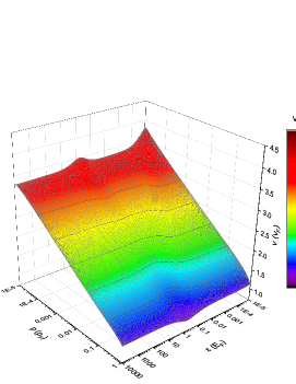
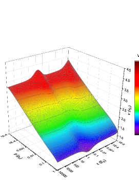
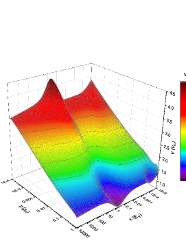
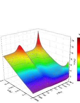
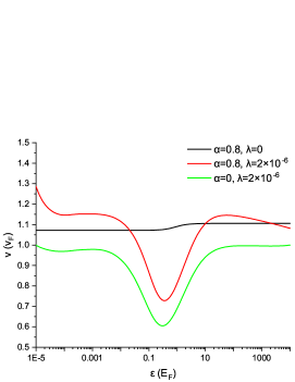
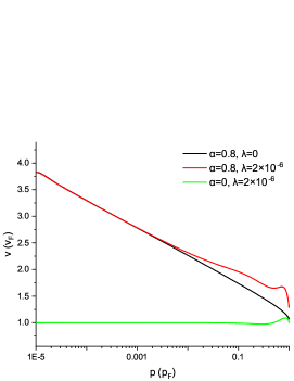
Figure 4: Full energy-momentum dependence of renormalized fermion velocity $v$ are presented in (a-d). Phonon velocity is fixed at $c_{s}=1\times 10^{-4}$ (in unit of bare fermion velocity $v_{F}$). (a) $\lambda=0.5\times 10^{-6}$, $\alpha=0.8$. (b) $\lambda=1\times 10^{-6}$, $\alpha=0.8$. (c) $\lambda=2\times 10^{-6}$, $\alpha=0.8$. (d) $\lambda=1\times 10^{-6}$, $\alpha=2.2$. (e) Energy-dependence of $v$ as $|\mathbf{p}|\rightarrow p_{F}$. (f) Momentum-dependence of $v$ as $\epsilon\rightarrow 0$.

The numerical results of $v(\epsilon_{n},\mathbf{p})$ are plotted in Fig. 4. The energy (momentum) is in unit of Fermi energy $E_{F}$ (Fermi momentum $p_{F}$). One observes from Fig. 4(a-c) that $v(\epsilon_{n},\mathbf{p})$ exhibits a clear non-monotonic dependence on energy for any fixed $|\mathbf{p}|$ due to the interplay of two interactions. In comparison, as shown in Ref. Pan21 , $v$ is energy independent if we only consider the Coulomb interaction. Thus the non-monotonic energy-dependence of $v$ is dominantly induced by EPI. To see this fact more explicitly, we plot $v(\epsilon)$ in Fig. 4(e) in the $|\mathbf{p}|\rightarrow p_{F}$ limit. As the EPI strength parameter $\lambda$ increases, the non-monotonicity becomes more pronounced, which can be seen by comparing the results shown in Fig. 4(a-c).

Moreover, we find that $v$ is a decreasing function of $|\mathbf{p}|$ at any fixed energy for $\alpha=0.8$, no matter whether the effects of EPI are taken into account. For $\alpha=2.2$, $v$ first decreases with growing $|\mathbf{p}|$, but tends to increase as $|\mathbf{p}|$ approaches its ultraviolet cutoff. This upturn behavior is shown in Fig. 4(d). According to Fig. 4(f), EPI makes little contribution to the $|\mathbf{p}|$-dependence of $v$. In particular, adding EPI to the system does not change the logarithmic $|\mathbf{p}|$-dependence of $v(\mathbf{p})$ in the small-$|\mathbf{p}|$ region caused purely by the Coulomb interaction. This result provides a natural explanation of the surprisingly good agreement between the experimental result of $v(\mathbf{p})$ measured in realistic graphene materials Elias11 ; Lanzara11 ; Chae12 and the theoretical result of $v(\mathbf{p})$ calculated without taking into account the impact of EPI Gonzalez94 ; Pan21 . We see from Fig. 4(a-d) that the renormalized velocity $v$ seems to increase abruptly if $\epsilon\to 0$ and $|\mathbf{p}|\rightarrow 0$. As discussed in Ref. Pan21 , this is an artifact caused by infrared cutoffs and the logarithmic $|\mathbf{p}|$-dependence of fermion velocity is actually robust in the small-$|\mathbf{p}|$ region as the infrared cutoffs of $\epsilon$ and $|\mathbf{p}|$ decrease. Different from the small-$|\mathbf{p}|$ region, EPI can drive $v(\mathbf{p})$ to deviate from the standard logarithmic behavior in large-$|\mathbf{p}|$ region.

Once the full fermion propagator $G(p)$ is determined, one can proceed to analyze the interaction effects on the properties of bosons. According the analytical computations presented in Appendix B, the DS equation of full phonon propagator $D(q)$ and that of full $A$ boson propagator $F(q)$ are

$$D(q) = D_{0}(q)\Big{[}1-iN\int dpD_{0}(q)g^{2}\mathrm{Tr}\big{[}G(p+q)\Gamma_{0}(q,p)G(p)\big{]}\Big{]},$$ (100)

$$F(q) = F_{0}(q)\Big{[}1-iN\int dpF_{0}(q)\mathrm{Tr}\big{[}G(p+q)\Gamma_{0}(q,p)G(p)\big{]}\Big{]},$$ (101)

which are derived from Eq. (117) and Eq. (118), respectively. The equations of $D(q)$ and $F(q)$ are no longer self-consistent, and can be directly computed once the full fermion propagator $G(p)$ is obtained by solving its DS equation. The polarization functions $\Pi_{p}(q)$ and $\Pi_{A}(q)$, namely the self-energy functions of phonons and Coulomb interaction, can also be calculated by using $D(q)$ and $F(q)$, as shown by Eq. (126) and Eq. (127). More details about the interaction effects on bosons can be found in Appendix B. While these issues are interesting and deserve further investigations, they apparently have no influence on the renormalization of fermion velocity and will be addressed in separate works.

V Summary and Discussion

In summary, here we present a non-perturbative study of the interplay of EPI and Coulomb interaction in the context of graphene by using the DS equation approach. In previous works, the effects of EPI and Coulomb interaction are usually studied separately. When both interactions are important, the situation becomes much more involved. In this paper, we rigorously derive the DS equation of the fully dressed Dirac fermion propagator $G(p)$ by taking into account the interplay of EPI and Coulomb interaction. This equation is given by Eq. (27). As far as we know, such an equation has not been obtained in previous publications. After carrying out a careful analysis, we find that the correlation functions appearing in the DS equation of $G(p)$ obey a number of exact identities, including Eq. (40), Eq. (41), and Eqs. (69). All of these identities are derived from the invariance of the partition function under various infinitesimal changes of the fermionic and bosonic operators. Based on these identities, we prove that the DS equation of $G(p)$ is indeed self-closed. This is the main new result of this work.

As an application of our approach, we study how the fermion velocity is renormalized. By numerically solving the self-closed DS equation of $G(p)$ by means of iteration method, we show that the momentum dependence and the energy dependence of the renormalized fermion velocity is dominantly determined by the Coulomb interaction and the EPI, respectively. In particular, the renormalized velocity $v(\mathbf{p})$ exhibits a logarithmic $|\mathbf{p}|$-dependence over a broad range of $|\mathbf{p}|$. This theoretical result is in good agreement with the existing experiments of graphene Elias11 ; Lanzara11 ; Chae12 .

We now comment on the range of applicability of our approach. To make the DS equation of $G(p)$ self-closed, it is necessary to derive a sufficient number of WTIs. In the model considered in this work, there is only one coupling term for each FBI, namely $\phi\bar{\psi}\gamma_{0}\psi$ for EPI and $A\bar{\psi}\gamma_{0}\psi$ for Coulomb interaction. One can find enough matrices to eliminate the special correlation functions appearing in r.h.s. of Eq. (45). For a FBI term that has more than one components, it would be hard to eliminate such correlation functions. Let us take relativistic QED₄ Itzykson as an example. The Lagrangian density of QED₄ is given by

$$\mathcal{L}_{\mathrm{QED}}=\sum_{\sigma}^{N}\bar{\psi}_{\sigma}\gamma^{\mu}\left(i\partial_{\mu}-ea_{\mu}\right)\psi_{\sigma}-\frac{1}{4}F^{\mu\nu}F_{\mu\nu},$$ (102)

where $\psi$ is a four-component spinor and $a_{\mu}$ is an abelian gauge field. $F_{\mu\nu}=\partial_{\mu}a_{\nu}-\partial_{\nu}a_{\mu}$ is the electricmagnetic tensor. Different from EPI and Coulomb interaction, the gauge interaction term is composed of four components, namely $a_{\mu}\bar{\psi}\gamma^{\mu}\psi$ with $\mu=0,1,2,3$. Let the spinor field transform as $\psi\to e^{i\theta\gamma^{m}}\psi$, where $\theta$ is an infinitesimal constant and $\gamma^{m}$ could be any $4\times 4$ matrix. On the basis of the invariance of the partition function $Z$ under such transformations, one would obtain an identity analogous to Eq. (44). Such an identity would contain the following term

$$\langle a_{\mu}(x){\bar{\psi}}_{\sigma}(x)(\gamma^{\mu}\gamma^{m}-\gamma^{m}\gamma^{\mu})\psi_{\sigma}(x)\psi(y){\bar{\psi}}(z)\rangle.$$ (103)

There are not enough $\gamma^{m}$ matrices to fulfill the constraint $\gamma^{\mu}\gamma^{m}-\gamma^{m}\gamma^{\mu}=0$ for all the four components of $\gamma^{\mu}$. Thus the above correlation function cannot be simply eliminated. It then becomes difficult to prove that the DS equation of the full fermion propagator is self-closed. The same difficulty also exists in QED₃. In fact, such a difficulty is encountered in any quantum field theory in which the fermion-boson coupling has two or more components. For instance, when the spin degrees of freedom of Dirac fermions become important, we need to consider such a coupling term as $\psi^{{\dagger}}\mathbf{\gamma}\cdot\psi\mathbf{S}$, where $\mathbf{S}$ is a three-dimensional spin operator. We should further generalize our approach to deal with these complicated models.

Appendix A Derivation of the interaction vertex functions

Here we show how to use the fermion and boson propagators (two-point correlation functions) to express the following (connected) three-point correlation function:

$$\langle\phi(x)\psi_{\sigma}(y)\bar{\psi}_{\sigma}(z)\rangle_{c} = \frac{\delta^{3}W}{\delta J(x)\delta\bar{\eta}_{\sigma}(y)\delta\eta_{\sigma}(z)}\Big{|}_{J=0}.$$ (104)

According to the elementary rules of function integral Itzykson , we re-write the above expression as

$$\frac{\delta^{3}W}{\delta J(x)\delta\bar{\eta}_{\sigma}(y)\delta\eta_{\sigma}(z)}\Big{|}_{J=0} = \frac{\delta}{\delta J(x)}\Big{|}_{J=0}\frac{\delta^{2}W}{\delta\bar{\eta}_{\sigma}(y)\delta\eta_{\sigma}(z)}$$ (105)

$$= -\frac{\delta}{\delta J(x)}\Big{|}_{J=0}\left(\frac{\delta^{2}\Xi}{\delta\bar{\psi}_{\sigma}(y)\delta\psi_{\sigma}(z)}\right)^{-1}$$

$$= \int dy^{\prime}dz^{\prime}\left(\frac{\delta^{2}\Xi}{\delta\bar{\psi}_{\sigma}(y)\delta\psi_{\sigma}(y^{\prime})}\right)^{-1}$$

$$\times\left[\frac{\delta}{\delta J(x)}\Big{|}_{J=0}\frac{\delta^{2}\Xi}{\delta\bar{\psi}_{\sigma}(y^{\prime})\delta\psi_{\sigma}(z^{\prime})}\right]\left(\frac{\delta^{2}\Xi}{\delta\bar{\psi}_{\sigma}(z^{\prime})\delta\psi_{\sigma}(z)}\right)^{-1},$$

The operator $\frac{\delta}{\delta J(x)}\Big{|}_{J=0}$ appearing in Eq. (105) needs to be treated carefully. It can be expanded as

$$\frac{\delta}{\delta J(x)}\Big{|}_{J=0} = \frac{\delta\phi}{\delta J}\Big{|}_{J=0}\frac{\delta}{\delta\phi}\Big{|}_{J=0}+\frac{\delta A}{\delta J}\Big{|}_{J=0}\frac{\delta}{\delta A}\Big{|}_{J=0}+\sum_{\sigma}^{N}\left(\frac{\delta\bar{\psi}_{\sigma}}{\delta J}\Big{|}_{J=0}\frac{\delta}{\delta\bar{\psi}_{\sigma}}\Big{|}_{J=0}+\frac{\delta\psi_{\sigma}}{\delta J}\Big{|}_{J=0}\frac{\delta}{\delta\psi_{\sigma}}\Big{|}_{J=0}\right)$$ (106)

$$= i\langle\phi\phi\rangle_{c}\frac{\delta}{\delta\phi}\Big{|}_{J=0}+i\langle\phi A\rangle_{c}\frac{\delta}{\delta A}\Big{|}_{J=0}+\sum_{\sigma}^{N}\left(\langle\phi\bar{\psi}_{\sigma}\rangle_{c}\frac{\delta}{\delta\bar{\psi}_{\sigma}}\Big{|}_{J=0}+\langle\phi\psi_{\sigma}\rangle_{c}\frac{\delta}{\delta\psi_{\sigma}}\Big{|}_{J=0}\right)$$

$$= -D\frac{\delta}{\delta\phi}\Big{|}_{J=0}-D_{F}\frac{\delta}{\delta A}\Big{|}_{J=0}+0+0.$$

It is obviously true that $\langle\phi\bar{\psi}_{\sigma}\rangle_{c}=\langle\phi\psi_{\sigma}\rangle_{c}=0$ when all external sources are removed because a fermion (boson) cannot be converted into a boson (fermion) without inducing additional changes. However, one cannot simply set $\langle\phi A\rangle_{c}=0$. Although there is no direct coupling between $\phi$ and $A$ bosons in the Lagrangian density (tree-level), they are both coupled to fermions and thus can be turned into each other via quantum corrections (loop-level). Phonons result from the lattice vibration and EPI basically describes the mutual influence between negatively charged fermions and positively charged ions. On the other hand, the Coulomb interaction is experienced by negatively charged fermions. As the ions are vibrating, the resultant phonon excitations affect the surrounding electric field of fermions, which in turn alters the Coulombic potential between fermions. These processes are embodied in such correlation function as $\langle\phi A\rangle$ and $\langle A\phi\rangle$. Substituting the above expression of $\frac{\delta}{\delta J(x)}\Big{|}_{J=0}$ into Eq. (105) leads to

$$\frac{\delta^{3}W}{\delta J(x)\delta\bar{\eta}_{\sigma}(y)\delta\eta_{\sigma}(z)}\Big{|}_{J=0}$$ (107)

$$= -\int dx^{\prime}dy^{\prime}dz^{\prime}\left(\frac{\delta^{2}\Xi}{\delta\bar{\psi}_{\sigma}(y)\delta\psi_{\sigma}(y^{\prime})}\right)^{-1}$$

$$\times\left[\left(D(x-x^{\prime})\frac{\delta}{\delta\phi(x^{\prime})}\Big{|}_{J=0}+D_{F}(x-x^{\prime})\frac{\delta}{\delta A(x^{\prime})}\Big{|}_{J=0}\right)\frac{\delta^{2}\Xi}{\delta\bar{\psi}_{\sigma}(y^{\prime})\delta\psi_{\sigma}(z^{\prime})}\right]\left(\frac{\delta^{2}\Xi}{\delta\bar{\psi}_{\sigma}(z^{\prime})\delta\psi_{\sigma}(z)}\right)^{-1}$$

$$= -\int dx^{\prime}dy^{\prime}dz^{\prime}D(x-x^{\prime})G(y-y^{\prime})\frac{\delta^{3}\Xi}{\delta\phi(x^{\prime})\delta\bar{\psi}_{\sigma}(y^{\prime})\delta\psi_{\sigma}(z^{\prime})}\Big{|}_{J=0}G(z^{\prime}-z)$$

$$-\int dx^{\prime}dy^{\prime}dz^{\prime}D_{F}(x-x^{\prime})G(y-y^{\prime})\frac{\delta^{3}\Xi}{\delta A(x^{\prime})\delta\bar{\psi}_{\sigma}(y^{\prime})\delta\psi_{\sigma}(z^{\prime})}\Big{|}_{J=0}G(z^{\prime}-z).$$

The two-point correlation functions $G$, $D$, and $D_{F}$ are already defined in Sec. II.

Appendix B Derivation of the DS equations of fermion and boson propagators

We first derive the DS equation of the full fermion propagator $G(p)$, taking into account the corrections from two different FBIs. The partition function $Z$ is invariant under an arbitrary infinitesimal change $\delta\bar{\psi}_{\sigma}$. This feature can be used to obtain an identity

$$\langle\left(i\partial_{0}\gamma_{0}-i\partial_{1}\gamma_{1}-i\partial_{2}\gamma_{2}\right)\psi_{\sigma}(x)-g\phi(x)\gamma_{0}\psi_{\sigma}(x)-A(x)\gamma_{0}\psi_{\sigma}(x)+\eta_{\sigma}(x)\rangle=0.$$ (108)

It is convenient to express this identity in terms of the generating functional $W$ as follows

$$(i\partial_{0}\gamma_{0}-i\partial_{1}\gamma_{1}-i\partial_{2}\gamma_{2})\frac{\delta W}{\delta\bar{\eta}_{\sigma}(x)}+ig\gamma_{0}\frac{\delta^{2}W}{\delta J(x)\delta\bar{\eta}_{\sigma}(x)}-g\gamma_{0}\frac{\delta W}{\delta J(x)}\frac{\delta W}{\delta\bar{\eta}_{\sigma}(x)}$$

$$+i\gamma_{0}\frac{\delta^{2}W}{\delta A(x)\delta\bar{\eta}_{\sigma}(x)}-\gamma_{0}\frac{\delta W}{\delta A(x)}\frac{\delta W}{\delta\bar{\eta}_{\sigma}(x)}+\eta_{\sigma}(x)=0.$$ (109)

Applying the variation $-\frac{\delta}{\delta\eta_{\sigma}(y)}\Big{|}_{J=0}$ to this identity, we obtain

$$\delta(x-y)=(i\partial_{0}\gamma_{0}-i\partial_{1}\gamma_{1}-i\partial_{2}\gamma_{2})\frac{\delta^{2}W}{\delta\bar{\eta}_{\sigma}(x)\delta\eta_{\sigma}(y)}+ig\gamma_{0}\langle\phi(x)\psi_{\sigma}(x)\bar{\psi}_{\sigma}(y)\rangle_{c}+i\gamma_{0}\langle A(x)\psi_{\sigma}(x)\bar{\psi}_{\sigma}(y)\rangle_{c}.$$

Substituting Eq. (23) and Eq. (24) into it and making Fourier transformation give rise to

$$1 = (p_{0}\gamma_{0}-\mathbf{\gamma\cdot p})G(p)-i\int_{q}g\gamma_{0}D(q)G(p+q)\Gamma_{p}(q,p)G(p)-i\int_{q}g\gamma_{0}D_{F}(q)G(p+q)\Gamma_{A}(q,p)G(p)$$ (111)

$$-i\int_{q}\gamma_{0}F_{D}(q)G(p+q)\Gamma_{p}(q,p)G(p)-i\int_{q}g\gamma_{0}F(q)G(p+q)\Gamma_{A}(q,p)G(p).$$

This equation can be re-written in a more compact form

$$G^{-1}(p) = G_{0}^{-1}(p)-i\int_{q}g\gamma_{0}G(p+q)D(q)\Gamma_{p}(q,p)-i\int_{q}\gamma_{0}G(p+q)F(q)\Gamma_{A}(q,p)$$ (112)

$$-i\int_{q}g\gamma_{0}G(p+q)D_{F}(q)\Gamma_{A}(q,p)-i\int_{q}\gamma_{0}G(p+q)F_{D}(q)\Gamma_{p}(q,p).$$

Apparently, this equation is independent of the fermion flavor index $\sigma$. In other words, the fermion propagator $G_{\sigma}(p)$ for each flavor $\sigma$ satisfies the same DS equation.

Then we derive the DS equations satisfied by the full boson propagators. As usual, we first work with the real time and the real energy and finally replace the real energy with the imaginary Matsubara frequency.

When one makes an arbitrary infinitesimal change of the phonon field $\phi$, the partition function $Z$ should not change. This allows us to obtain an equation

$$\langle\mathbb{D}\phi(x)-ig\sum_{\sigma}^{N}\bar{\psi}_{\sigma}(x)\gamma_{0}\psi_{\sigma}(x)\rangle+J(x)=0,$$ (113)

which is equivalent to

$$\mathbb{D}\frac{\delta W}{\delta J(x)}+i\sum_{\sigma}^{N}g\mathrm{Tr}\left[\gamma_{0}\frac{\delta^{2}W}{\delta\bar{\eta}_{\sigma}(x)\delta\eta_{\sigma}(x)}\right]+J(x)=0.$$ (114)

Perform a functional derivative $\frac{\delta}{\delta J(y)}|_{J=0}$ to both sides of this equation leads to

$$\mathbb{D}D(x-y)+iN\int dzdz^{\prime}dy^{\prime}gD(y-y^{\prime})\mathrm{Tr}[\gamma_{0}G(x-z)\frac{\delta^{3}\Xi}{\delta\phi(y^{\prime})\delta\bar{\psi}_{\sigma}(z)\delta\psi_{\sigma}(z^{\prime})}\Big{|}_{J=0}G(z^{\prime}-x)]$$

$$+iN\int dzdz^{\prime}dy^{\prime}gD_{F}(y-y^{\prime})\mathrm{Tr}\left[\gamma_{0}G(x-z)\frac{\delta^{3}\Xi}{\delta\phi(y^{\prime})\delta\bar{\psi}_{\sigma}(z)\delta\psi_{\sigma}(z^{\prime})}\Big{|}_{J=0}G(z^{\prime}-x)\right]-\delta(x-y)=0.$$

We now substitute Eq. (II) into this equation and then carry out Fourier transformations. The full phonon propagator $D(q)$ is found to satisfy the following DS equation

$$D_{0}^{-1}(q)D(q)+iN\int dpD(q)g\mathrm{Tr}[G(p+q)\Gamma_{p}(q,p)G(p)]$$

$$+iN\int dpD_{F}(q)g\mathrm{Tr}[G(p+q)\Gamma_{A}(q,p)G(p)]=1.$$ (116)

This DS equation is formally very complicated. Fortunately, using the identity given by Eq. (40), we find that the DS equation of $D(q)$ can be substantially simplified into

$$D_{0}^{-1}(q)D(q)+iN\int dpD_{0}(q)g^{2}\mathrm{Tr}[G(p+q)\Gamma_{0}(q,p)G(p)]=1.$$ (117)

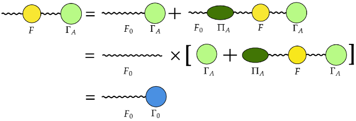
Figure 5: A schematic illustration of the relation satisfied by $\Gamma_{0}(q,p)$ and $\Pi_{A}(q)$.

Then we apply the above derivational procedure to the other boson field $A$ and, after repeating similar calculations, obtain the DS equation of the full $A$ boson propagator $F(q)$:

$$F_{0}^{-1}(q)F(q)+iN\int dpF_{0}(q)\mathrm{Tr}[G(p+q)\Gamma_{0}(q,p)G(p)]=1.$$ (118)

The polarization functions, i.e., the self-energy functions, of the phonons and the Coulomb interaction can be calculated as follows:

$$\Pi_{p}(q) = D_{0}^{-1}(q)-D^{-1}(q),$$ (119)

$$\Pi_{A}(q) = F_{0}^{-1}(q)-F^{-1}(q).$$ (120)

Let us take $\Pi_{A}(q)$ as an example to illustrate how the current vertex function $\Gamma_{0}(q,p)$ is related to the polarization function. In the absence of phonons, the identity Eq. (41) becomes

$$F(q)\Gamma_{A}(q,p)=F_{0}(q)\Gamma_{0}(q,p).$$ (121)

Making use of Eq. (120), this identity is converted into

$$F(q)\Gamma_{A}(q,p) = \left[F_{0}(q)+F_{0}(q)\Pi_{A}(q)F(q)\right]\Gamma_{A}(q,p)$$ (122)

$$= F_{0}(q)\left[1+\Pi_{A}(q)F(q)\right]\Gamma_{A}(q,p)$$

$$= F_{0}(q)\Gamma_{0}(q,p).$$

This derivational process can be intuitively illustrated by the diagrams plotted in Fig. 5. It is now obvious that $\Gamma_{0}(q,p)$ depends on $\Pi_{A}(q)$ via the relation

$$\Gamma_{0}(q,p)=\left[1+\Pi_{A}(q)F(q)\right]\Gamma_{A}(q,p).$$ (123)

The fermion flavor $N$ enters into $\Pi_{A}(q)$ and also into $F(q)$. However, $\Gamma_{0}(q,p)$ is independent of $N$, as shown by Eq. (71). It can be inferred that the $N$-dependence of $1+\Pi_{A}(q)F(q)$ cancels that of $\Gamma_{A}(q,p)$.

It is appropriate at this stage to transform real energy into imaginary frequency. After doing so we re-write the two full boson propagators as

$$D(\omega_{n^{\prime}},\mathbf{q}) = D_{0}(\omega_{n^{\prime}},\mathbf{q})\Big{[}1+N\sum_{n}\int\frac{d^{2}\mathbf{q}}{(2\pi)^{2}}D_{0}(\omega_{n^{\prime}},\mathbf{q})g^{2}\mathrm{Tr}\big{[}G(\epsilon_{n^{\prime}+n},\mathbf{p+q})\Gamma_{0}(q,p)G(\epsilon_{n},\mathbf{p})\big{]}\Big{]},$$ (124)

$$F(\omega_{n^{\prime}},\mathbf{q}) = F_{0}(\omega_{n^{\prime}},\mathbf{q})\Big{[}1+N\sum_{n}\int\frac{d^{2}\mathbf{q}}{(2\pi)^{2}}F_{0}(\omega_{n^{\prime}},\mathbf{q})\mathrm{Tr}\big{[}G(\epsilon_{n^{\prime}+n},\mathbf{p+q})\Gamma_{0}(q,p)G(\epsilon_{n},\mathbf{p})\big{]}\Big{]}.$$ (125)

The full propagators can be used to compute the polarization functions. Specifically, the polarization function for phonons is

$$\Pi_{p}(\omega_{n^{\prime}},\mathbf{q}) = D_{0}^{-1}(\omega_{n^{\prime}},\mathbf{q})-D^{-1}(\omega_{n^{\prime}},\mathbf{q})$$ (126)

$$= \frac{N\sum_{n}\int\frac{d^{2}\mathbf{q}}{(2\pi)^{2}}g^{2}\mathrm{Tr}\big{[}G(\epsilon_{n^{\prime}+n},\mathbf{p+q})\Gamma_{0}(q,p)G(\epsilon_{n},\mathbf{p})\big{]}}{1+N\sum_{n}\int\frac{d^{2}\mathbf{q}}{(2\pi)^{2}}D_{0}(\omega_{n^{\prime}},\mathbf{q})g^{2}\mathrm{Tr}\big{[}G(\epsilon_{n^{\prime}+n},\mathbf{p+q})\Gamma_{0}(q,p)G(\epsilon_{n},\mathbf{p})\big{]}},$$

and the polarization function for $A$ boson (Coulomb interaction) is

$$\Pi_{A}(\omega_{n^{\prime}},\mathbf{q}) = F_{0}^{-1}(\omega_{n^{\prime}},\mathbf{q})-F^{-1}(\omega_{n^{\prime}},\mathbf{q})$$ (127)

$$= \frac{N\sum_{n}\int\frac{d^{2}\mathbf{q}}{(2\pi)^{2}}\mathrm{Tr}\big{[}G(\epsilon_{n^{\prime}+n},\mathbf{p+q})\Gamma_{0}(q,p)G(\epsilon_{n},\mathbf{p})\big{]}}{1+N\sum_{n}\int\frac{d^{2}\mathbf{q}}{(2\pi)^{2}}F_{0}(\omega_{n^{\prime}},\mathbf{q})\mathrm{Tr}\big{[}G(\epsilon_{n^{\prime}+n},\mathbf{p+q})\Gamma_{0}(q,p)G(\epsilon_{n},\mathbf{p})\big{]}}.$$

Based on the above results, in principle it would be straightforward to analyze the interaction effects on the behaviors of two bosons. For instance, the dielectric constant $\varepsilon$ becomes a function of energy and momentum, formally given by

$$\varepsilon(\omega_{n^{\prime}},\mathbf{q}) = 1-F_{0}(\omega_{n^{\prime}},\mathbf{q})\Pi_{A}(\omega_{n^{\prime}},\mathbf{q})$$ (128)

$$= \frac{1}{1+N\sum_{n}\int\frac{d^{2}\mathbf{q}}{(2\pi)^{2}}F_{0}(\omega_{n^{\prime}},\mathbf{q})\mathrm{Tr}\big{[}G(\epsilon_{n^{\prime}+n},\mathbf{p+q})\Gamma_{0}(q,p)G(\epsilon_{n},\mathbf{p})\big{]}}.$$

Moreover, one can investigate the properties of plasmon mode by studying the polarization functions and compute the renormalized phonon velocity $c_{s}$ based on the full phonon propagator $D(q)$. From the technical perspective, it is difficult to perform such calculations because one needs to first find an efficient numerical method to translate the functions obtained using imaginary frequencies into retarded and advanced functions that depend on real energies.

References

(1)
E. Abrahams, P. W. Anderson, D. C. Licciardello, and T. V.
Ramakrishnan, Phys. Rev. Lett. 42, 673 (1979).
(2)
A. M. Finkelstein, Z. Phys. B: Condens. Matter 56, 189 (1984); C.
Castellani, C. Di Castro, P. A. Lee, and M. Ma, Phys. Rev. B 30, 527 (1984).
(3)
E. Abrahams, S. V. Kravchenko, and M. P. Sarachik, Rev. Mod. Phys.
73, 251 (2001).
(4)
J. R. Schrieffer, Theory of Superconductivity (CRC Press,
2018).
(5)
A. Migdal, Sov. Phys. JETP 7, 996 (1958).
(6)
G. M. Eliashberg, Sov. Phys. JETP 11, 696 (1960).
(7)
D. J. Scalapino, The electron-phonon interaction and
strong-coupling superconductivity, in Superconductivity,
edited by R. D. Parks (Marcel Dekker, New York, 1969).
(8)
P. B. Allen and B. Mitrović, Theory of Superconducting
Tc, Solid State Physics, Vol. 37 (Academic Press, 1982).
(9)
F. Marsiglio, Ann. Phys. 417, 168102 (2020).
(10)
G.-Z. Liu, Z.-K. Yang, X.-Y. Pan, and J.-R. Wang, Phys. Rev. B 103, 094501 (2021).
(11)
X.-Y. Pan, Z.-K. Yang, X. Li, and G.-Z. Liu, Phys. Rev. B 104,
085141 (2021).
(12)
A. H. Castro Neto, F. Guinea, N. M. R. Peres, K. S. Novoselov, and
A. K. Geim, Rev. Mod. Phys. 81, 109 (2009).
(13)
S. Das Sarma, S. Adam, E. H. Hwang, and E. Rossi, Rev. Mod. Phys.
83, 407 (2011).
(14)
V. N. Kotov, B. Uchoa, V. M. Pereira, F. Guinea, and A. H. Castro
Neto, Rev. Mod. Phys. 84, 1067 (2012).
(15)
J. González, F. Guinea, and M. A. H. Vozmediano, Nucl. Phys. B
424, 595 (1994).
(16)
S. Das Sarma, E. H. Hwang, and W.-K. Tse, Phys. Rev. B 75,
121406(R) (2007).
(17)
M. Polini, R. Asgari, Y. Barlas, T. Pereg-Barnea, and A. H.
MacDonald, Solid State Commun. 143, 58 (2007).
(18)
D. T. Son, Phys. Rev. B 75, 235423 (2007).
(19)
O. Vafek, Phys. Rev. Lett. 98, 216401 (2007).
(20)
E. G. Mishchenko, Phys. Rev. Lett. 98, 216801 (2007).
(21)
O. Vafek and M. J. Case, Phys. Rev. B 77, 033410 (2008).
(22)
J. E. Drut and D. T. Son, Phys. Rev. B 77, 075115 (2008).
(23)
D. M. Basko and I. L. Aleiner, Phys. Rev. B 77, 041409(R)
(2008).
(24)
M. S. Foster and I. L. Aleiner, Phys. Rev. B 77, 195413
(2008).
(25)
V. N. Kotov, B. Uchoa, and A. H. Castro Neto, Phys. Rev. B 78,
035119 (2008).
(26)
V. N. Kotov, B. Uchoa, and A. H. Castro Neto, Phys. Rev. B 80,
165424 (2009).
(27)
F. de Juan, A. G. Grushin, and M. A. H. Vozmediano, Phys. Rev. B
82, 125409 (2010).
(28)
M. A. H. Vozmediano, Phil. Trans. R. Soc. A. 369, 2625-2642
(2011).
(29)
I. Sodemann and M. M. Fogler, Phys. Rev. B 86, 115408 (2012).
(30)
J. Hofmann, E. Barnes, and S. Das Sarma, Phys. Rev. Lett. 113,
105502 (2014).
(31)
E. Barnes, E. H. Hwang, R. E. Throckmorton, and S. Das Sarma, Phys.
Rev. B 89, 235431 (2014).
(32)
R. E. Throckmorton, J. Hofmann, E. Barnes, and S. Das Sarma, Phys.
Rev. B 92, 115101 (2015).
(33)
A. Sharma and P. Kopietz, Phys. Rev. B 93, 235425 (2016).
(34)
D. V. Khveshchenko, Phys. Rev. Lett. 87, 246802 (2001).
(35)
E. V. Gorbar, V. P. Gusynin, V. A. Miransky, and I. A. Shovkovy,
Phys. Rev. B 66, 045108 (2002).
(36)
D. V. Khveshchenko and H. Leal, Nucl. Phys. B 687, 323 (2004).
(37)
D. V. Khveshchenko, J. Phys.: Condens. Matter 21, 075303
(2009).
(38)
G.-Z. Liu, W. Li, and G. Cheng, Phys. Rev. B 79, 205429
(2009).
(39)
O. V. Gamayun, E. V. Gorbar, and V. P. Gusynin, Phys. Rev. B 81, 075429 (2010).
(40)
J.-R. Wang and G.-Z. Liu, New J. Phys. 14, 043036 (2012).
(41)
J.-R. Wang and G.-Z. Liu, Phys. Rev. B 89, 195404 (2014).
(42)
J. González, Phys. Rev. B 85, 085420 (2012).
(43)
J. González, JHEP 92, 027 (2012).
(44)
C. Popovici, Mod. Phys. Lett. A 28, 1330006 (2013).
(45)
M. E. Carrington, C. S. Fischer, L. von Smekal, and M. H. Thoma,
Phys. Rev. B 94, 125102 (2016).
(46)
M. E. Carrington, C. S. Fischer, L. von Smekal, and M. H. Thoma,
Phys. Rev. B 97, 115411 (2018).
(47)
D. C. Elias, R. V. Gorbachev, A. S. Mayorov, S. V. Morozov, A. A.
Zhukov, P. Blake, L. A. Ponomarenko, I. V. Grigorieva, K. S.
Novoselov, F. Guinea, and A. K. Geim, Nat. Phys. 7, 701
(2011).
(48)
D. A. Siegel, C.-H. Park, C. Hwang, J. Deslippe, A. V. Fedorov, S.
G. Louie, and A. Lanzara, Proc. Natl. Acad. Sci. U.S.A. 108,
11365 (2011).
(49)
J. Chae, S. Jung, A. F. Young, C. R. Dean, L. Wang, Y. Gao, K.
Watanabe, T. Taniguchi, J. Hone, K. L. Shepard, P. Kim, N. B.
Zhitenev, and J. A. Stroscio, Phys. Rev. Lett. 109, 116802
(2012).
(50)
C.-H. Park, F. Giustino, M. L. Cohen, and S. G. Louie, Phys. Rev.
Lett. 99, 086804 (2007).
(51)
W.-K. Tse and S. Das Sarma, Phys. Rev. Lett. 99, 236802
(2007).
(52)
B. Roy, J. D. Sau, and S. Das Sarma, Phys. Rev. B 89, 165119
(2014).
(53)
C. Chen, X. Y. Xu, Z. Y. Meng, and M. Hohenadler, Phys. Rev. Lett.
122, 077601 (2019).
(54)
Y.-X. Zhang, W.-T. Chiu, N. C. Costa, G. G. Batrouni, and R. T.
Scalettar, Phys. Rev. Lett. 122, 077602 (2019).
(55)
C. Itzykson and J.-B. Zuber, Quantum Field Theory
(McGraw-Hill, New York, 1980).
(56)
P. A. M. Dirac, Proc. Camb. Phil. Soc. 30, 150 (1934).
(57)
J. Schwinger, Phys. Rev. 82, 664 (1951).
(58)
R. Jackiw and K. Johnson, Phys. Rev. 182, 1459 (1969).
(59)
Y. Takahashi, Nuovo Cimento 47A, 392 (1978).
(60)
J. Novotny and M. Schnabl, Fortschr. Phys. 48, 253 (2000).
(61)
M. E. Peskin and D. V. Schroeder, An Introduction to Quantum
Field Theory (CRC Press, 2018).
(62)
H. He, F. C. Khanna, and Y. Takahashi, Phys. Lett. B 480, 222
(2000).
(63)
J. Ye and S. Sachdev, Phys. Rev. Lett. 80, 5409 (1998).
(64)
I. F. Herbut, Phys. Rev. Lett. 97, 146401 (2006).