Balsa: Learning a Query Optimizer Without Expert Demonstrations

Abstract.

Query optimizers are a performance-critical component in every database system. Due to their complexity, optimizers take experts months to write and years to refine. In this work, we demonstrate for the first time that learning to optimize queries without learning from an expert optimizer is both possible and efficient. We present Balsa, a query optimizer built by deep reinforcement learning. Balsa first learns basic knowledge from a simple, environment-agnostic simulator, followed by safe learning in real execution. On the Join Order Benchmark, Balsa matches the performance of two expert query optimizers, both open-source and commercial, with two hours of learning, and outperforms them by up to $2.8\times$ in workload runtime after a few more hours. Balsa thus opens the possibility of automatically learning to optimize in future compute environments where expert-designed optimizers do not exist.

1. Introduction

Query optimizers are a performance-critical component in every database and query engine, translating declarative queries into efficient execution plans. These optimizers must navigate a vast search space of candidate plans for each query, scoring each plan with sufficient accuracy by leveraging statistics about the data.

As a result of this complexity, optimizers are costly to develop. Human experts may spend months to write a first version and years to refine it. For example, PostgreSQL, one of the most widely used databases in the world, has seen a continuous stream of changes to its optimizer more than 20 years after it was released (developers, [n. d.]). Due to the high development costs, some relational systems settle for heuristic-based optimizations and postpone building full-fledged cost-based optimizers. As examples, Spark SQL was introduced in 2014 but only added a cost-based optimizer (CBO) in 2017, while CockroachDB shipped the first version of its CBO in v2.1 after “9 months of intense effort” (Kimball, 2018).

Instead of having human experts spend years developing a state-of-the-art optimizer, in this paper we ask whether it is possible to use machine learning to learn to optimize queries without learning from an existing expert optimizer. We answer this question affirmatively by designing and implementing Balsa, a learned query optimizer that can match or even exceed the performance of expert-built query optimizers (both open-source and commercial).

Balsa leverages deep reinforcement learning (RL), which has been successfully employed to learn complex skills (Akkaya et al., 2019) and exceed human experts at playing games (Silver et al., 2016, 2017; Vinyals et al., 2019). RL consists of an agent that learns to solve a task by repeatedly interacting with an environment. The agent observes the environment’s state and takes an action to maximize a reward. If the actions lead to improved rewards, they are reinforced, i.e., the agent is updated to make these actions more likely in the future. For a learned optimizer agent, such as Balsa, the environment is the database; a state is a partial plan for a query; an action is to add operators to the partial plan, and the reward for a complete plan is its execution latency (negated). Using this feedback loop, Balsa learns by trial and error to become increasingly better at generating query execution plans.

In fact, the promise of RL for query optimization has been shown by several recent projects (Krishnan et al., 2018; Marcus et al., 2019, 2021). However, these methods assume the availability of a mature query optimizer to learn from. In contrast, Balsa does not learn from such an expert optimizer. To our knowledge, Balsa demonstrates for the first time that learning to optimize queries without learning from an expert optimizer is both possible and efficient. This can have a far reaching impact, as it paves the road towards automatically learning to optimize in new data systems (Petersohn et al., 2020; Narayan, 2020) where a mature optimizer does not exist.

A unique challenge in learning to optimize queries without an expert optimizer’s guidance is that most execution plans for a query are slow—sometimes orders of magnitude more expensive than the optimal plan (Leis et al., 2015, 2018). At the beginning of the learning process, the agent has no prior knowledge, so the probability of selecting such disastrous plans is high, which may prevent any progress. This is a unique characteristic of query optimization that is not shared by other successful RL applications such as games. Indeed, with most games (e.g., AlphaGo (Silver et al., 2016), MuZero (Schrittwieser et al., 2020)), a “bad” action typically leads to a game ending quicker. As a result, bad actions do not hinder learning in those environments.

To avoid disastrous plans, Balsa employs simulation-to-reality learning (Tobin et al., 2017). In the “simulation” phase, Balsa quickly learns from a simulator how to avoid disastrous plans without executing queries, while in the “reality” phase it learns from real executions to produce high-performance plans. The simulator gives cost feedback to the agent by using a basic, logical-only cost model with a cardinality estimator. For convenience, we use PostgreSQL’s cardinality estimator, a simple histogram-based method (Leis et al., 2015). We pick an existing estimator since, unlike an optimizer, a cardinality estimator is agnostic to the execution environment, so the same estimator can be used for any environment. (In our evaluation, we use PostgreSQL’s estimates for another commercial engine.) Moreover, the estimator needs not be high-quality for effective simulation. In fact, PostgreSQL’s estimates can exhibit orders of magnitude errors (Leis et al., 2015), and we find that even injecting noises to these estimates does not impact Balsa’s performance (§10). This is because Balsa only uses the simulation to learn to avoid disastrous plans, not to reach expert-level performance. Therefore, basic cost models and estimates suffice.

Next, to vastly improve over the imperfect knowledge acquired from the simulator, Balsa learns in the real environment by actually executing queries. While the simulation knowledge enables the agent to avoid the worst plans, it can still stumble onto bad plans, causing unpredictable stalls in the learning process. Balsa addresses this challenge by using timeouts. A query’s timeout is set to its best latency so far during learning. If a plan times out, we assign it a predefined low reward (as we do not know its true reward). If the plan finishes, we tighten the timeout for future iterations. Thus, timeouts bound each learning iteration’s runtime, ensuring safe execution that eliminates unpredictable stalls.

Finally, an RL agent must balance exploiting past experiences with exploring new ones to escape local minima. The classic solution is random exploration, i.e., occasionally pick a random plan. Unfortunately, this standard strategy is ineffective, since random plans in the search space are likely to be highly expensive. Instead, Balsa explores from a set of probably good plans. During exploration, Balsa generates several best predicted plans (instead of the best), then picks the best unseen one out of them. This safe exploration approach improves Balsa’s plan coverage and performance.

Given a target dataset, Balsa is trained by repeatedly optimizing a set of sample queries by trial and error. After training, we test its generalization performance on a new set of unseen queries for the same dataset. We find that all three components of Balsa—simulation learning, safe execution, safe exploration—boost its generalization. They expose Balsa to a higher quantity and variety of plans, thereby enabling it to optimize new queries more robustly—a trait we believe is essential for the practical deployment of learned optimizers. We further propose using diversified experiences to enhance generalization (§6). We study Balsa’s generalization in depth in our evaluation (§8.2, §8.5), and find that it achieves better performance than two expert optimizers on unseen queries.

We call our approach “Bootstrap, Safely Execute, Safely Explore”, hence Balsa for short. To our knowledge, Balsa is the first learned optimizer that does not rely on plans (demonstrations) generated by an existing expert optimizer. On the Join Order Benchmark (Leis et al., 2015), a complex workload designed to stress test optimizers, Balsa matches the performance of two expert optimizers with two hours of training, and outperforms them by 2.1–2.8$\times$ after a few more hours.

In summary, we make the following contributions:

• We introduce Balsa, a learned query optimizer that does not learn from an existing, expert optimizer.

• We design a simple approach for learning a query optimizer without expert demonstrations: bootstrapping from simulation (§3), safe execution (§4), and safely exploring the plan space (§5).

• We propose diversified experiences, a novel method to further enhance training and generalization performance (§6), including generalizing to unseen queries with highly distinct join templates.

• Balsa can outperform both an open-source (PostgreSQL) and a commercial query optimizer, after a few hours of training (§8).

• We show that, despite not learning from an expert optimizer, Balsa outperforms the prior state-of-the-art technique that does.

Balsa is open sourced at https://github.com/balsa-project/balsa.

1.1. Differences from Prior Work

To highlight Balsa’s contributions, we briefly compare with the most related work and defer a complete discussion to §9.

DQ (Krishnan et al., 2018) learns from an expert optimizer’s cost model. As such, its performance is bounded by the quality of the cost model, which can be inaccurate. Neo (Marcus et al., 2019) takes an opposite approach by learning from an expert optimizer’s plans and real executions. While this is more accurate than using just a cost model, it is also more expensive. Importantly, these solutions assume either an expert cost model or an expert optimizer to bootstrap from.

In contrast, Balsa requires neither an expert cost model (as in DQ) nor an expert optimizer (as in Neo) to learn from. Balsa removes these fundamental assumptions by bootstrapping from a minimal, logical-only cost model, followed by safe learning in real execution. For the cost model, Balsa needs a basic cardinality estimator (§3.3). We find inaccurate estimates can still lead to successful simulation, and most of Balsa’s knowledge is learned after simulation (§10).

In summary, this paper tackles the new problem of learning to optimize when an expert optimizer does not exist. (We discuss in §10 how Balsa can better leverage an expert, if available, than prior work.) To solve this problem, we develop or apply techniques new to the domain of learned optimizers. These include sim-to-real (§2), safe execution (§4.3), safe exploration (§5), on-policy learning (§4.1), and enhancing generalization with diversified experiences (§6).

2. Balsa Overview

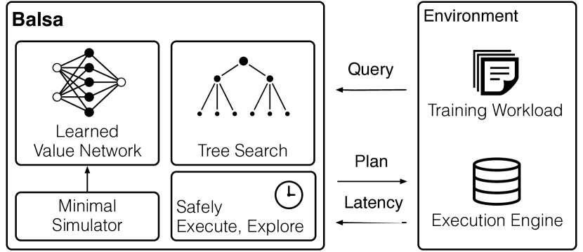
Figure 1. Balsa’s architecture. Balsa learns to optimize queries by executing plans and observing their latency feedback from an engine.

Balsa’s goal is to learn to optimize queries for a given dataset and an execution engine. We assume a training workload is available. At test time, Balsa is asked to optimize unseen queries issued for the same dataset, which can contain new filters and join graphs that are different from those in the training queries.

Balsa learns by trial and error. It optimizes the training queries, producing different plans, then executes them on the engine to observe their runtimes. Based on the runtime feedback, Balsa updates itself to correct mistakes and reward good decisions. As the feedback loop repeats, Balsa gets better at generating good plans.

After training, Balsa can be deployed to optimize an unseen test set of queries. The agent is evaluated by the performance of training plans produced, the performance of testing plans produced (i.e., its generalization ability), and its learning efficiency.

Throughout learning, Balsa accesses the underlying execution engine only to execute plans and observe their runtimes, and does not learn from an existing optimizer. This requirement is informed by the fact that many data systems have execution engines built long before an optimizer becomes available (§1).

Assumptions. We assume the database content is kept static. Updates to the schema, appends, or in-place updates can be handled by retraining. This assumption implies that the agent need not solve a learning problem with a shifting distribution. Another assumption is that Balsa currently optimizes select-project-join (SPJ) blocks. This is in line with the classical treatment (Selinger et al., 1979) of decomposing a query into simple SPJ blocks and optimizing them block-by-block.

2.1. Approach

Balsa’s architecture is shown in Figure 1. It consists of three basic components: bootstrapping a value network in a minimal cost model, fine-tuning the value network in real execution, and using a tree search algorithm to build query plans.

Classical design: cost models $+$ enumeration. The classical optimizer design (Selinger et al., 1979) uses an expert-implemented cost model that takes in a plan and outputs a cost estimate:

$$C:\textsf{plan}\rightarrow\textsf{cost}$$

Costs are designed to reflect real execution performance: lower costs should correlate with faster execution. The optimizer produces plans by enumerating candidate plans and scoring them using the cost model. For queries with a small number of tables, dynamic programming (DP) is typically used as the enumeration module.

RL: value functions $+$ planning. Instead of a cost model, which estimates the immediate cost of a plan, Balsa learns a value function that estimates the overall cost/latency of executing a query when the plan is used as a partial step (subplan):

$$V:(\textsf{query},\textsf{plan})\rightarrow\textsf{overall cost or latency}\\$$

Given a value function, we can use it to optimize queries by building a plan bottom-up. Consider a query $Q$ joining tables $\{A,B,C,D\}$. To figure out the best first join to perform, we compare the overall cost/latency, i.e., the value, of all valid first joins:

$$\{A,B,C,D\}\Rightarrow[V(Q,A\bowtie B));\,V(Q,A\bowtie C);\,\dots]$$

In other words, we use $V$ to score the 2-table joins, which are all partial subplans to complete query $Q$. The best first join is the one with the lowest $V$ value. Suppose $A\bowtie C$ is the best among them, then we can continue the process, scoring all possible second joins:

$$\{A\bowtie C,B,D\}\Rightarrow[V(Q,B\bowtie D);\,V(Q,B\bowtie(A\bowtie C));\,\dots]$$

Continuing such planning leads to a complete query plan.

In contrast to the classical cost model, a value function directly optimizes for the final, overall cost/latency of completing a query—the real objective we care about. Moreover, a learned value function can leverage data to tailor to a target database and hardware environment, potentially surpassing heuristics. If the optimal value function $V^{\ast}$ is known, then planning would produce optimal plans for queries. Our goal is to approximate $V^{\ast}$ as accurately as possible.

Learned value networks. Balsa approximates the optimal value function by training a neural network, $V_{\theta}(\textsf{query},\textsf{plan})$ (with parameters $\theta$), on agent-collected data. The two inputs to the network are featurized into query features (encoding joined tables and filters) and plan features (encoding the tree structure of the plan and each node’s operator type), respectively.

We learn the value function in two stages. First, we learn parameters $\theta_{\text{sim}}$ in a fast simulation environment backed by a minimal cost model. Next, we initialize parameters $\theta_{\text{real}}\leftarrow\theta_{\text{sim}}$ and start fine-tuning the value function in real execution. The two stages produce the value networks:

$$V_{\text{sim}} :(\textsf{query},\textsf{plan})\rightarrow\textsf{overall cost}$$

$$V_{\text{real}} :(\textsf{query},\textsf{plan})\rightarrow\textsf{overall latency}$$

After training, $V_{\text{real}}$ is used with planning to optimize new queries.

Step 1: bootstrapping from a minimal cost model (§3). Balsa starts learning in a “simulator” of query optimization, i.e., a cost model. The key advantage of using a simulator is that the agent can learn about disastrous plans without executing them in the initial phase of learning. The agent bootstraps initial knowledge against an inaccurate but fast-to-query cost model, which provides rapid feedback (cost estimates) for the agent. The cost model is generic and does not model the target engine or hardware.

To train the simulation model $V_{\text{sim}}$, we use a data collection procedure (e.g., DP) to enumerate plans for the training query set and ask the simulator for costs. Each query can yield thousands of training data points, eventually producing a sufficiently large dataset, $\mathcal{D}_{\text{sim}}=\{(\textsf{query},\textsf{plan},\textsf{overall cost})\}$. $V_{\text{sim}}$ is then trained on this dataset in a standard supervised learning fashion.

Step 2: fine-tuning in real execution (§4). Next, we transfer the value function from doing well in the simulator to excelling in the real execution environment. The second stage starts by initializing the real-execution model from the trained simulation model: $V_{\text{real}}$ $\leftarrow$ $V_{\text{sim}}$. The fine-tuning of $V_{\text{real}}$ is performed in iterations of query executions and model updates. In each iteration, Balsa uses its current $V_{\text{real}}$ to optimize training queries; these plans are executed with their latencies measured. Balsa then updates its $V_{\text{real}}$ on these collected data to make its latency predictions more accurate.

A key challenge of learning in real execution is mitigating slow plans. We address this as follows. By initializing from $V_{\text{sim}}$, Balsa’s behavior in iteration 0 would be much better than random initialization (which amounts to picking plans randomly). After iteration 0, Balsa uses timeouts (determined by earlier runtimes) to early-terminate slow plans (§4.3) and also employs safe exploration (§5).

Planning with tree search. Balsa uses tree search planning on top of the learned value function to optimize queries. The learned $V_{\text{real}}$ guides the search towards the promising regions of the plan space. As $V_{\text{real}}$ becomes more accurate, better plans can be found.

There are many tree search algorithms with different complexity-optimality tradeoffs: from greedy planning, to advanced planning algorithms such as Monte Carlo tree search. We opt for a middle ground by using a simple beam search (§4.2).

In the next sections, we describe Balsa’s components in detail.

3. Bootstrapping From Simulation

The first stage of training aims to rapidly impart basic knowledge to the agent, before it starts learning in long-running real executions. We achieve this by bootstrapping Balsa in a minimal simulator, i.e., a cost model. It “simulates” query optimization in that query plans are not actually executed. Instead, the agent issues a large amount of plans to the simulator, which can quickly return cost estimates (rather than measuring their runtimes) as feedback. Why is a simulator necessary? The search space for a query is vast and disastrous execution plans are abundant (Leis et al., 2015). Unfortunately, disastrous plans can stall learning progress: an agent may wait for a long time for a slow plan to complete execution, before learning that it is a bad action (if it ever finishes). This property is in direct contrast to other RL use cases such as games. In game environments (e.g., Go, chess, Atari), bad moves typically cause a game to end sooner, as the opponent can exploit the agent’s mistakes.

A randomly initialized RL agent without training in simulation can quite easily stumble upon such disastrous plans, especially in the early stage of learning. We show this with a simple experiment: we randomly initialize 6 agents without simulation learning, and task them with optimizing 94 queries from the Join Order Benchmark (detailed setup described in §8.1). Plans produced by the median random agent execute $45\times$ slower in workload runtime than those produced by an expert optimizer, PostgreSQL. The slowest agent is $79\times$ slower than the expert (2.5 hours vs. 2 minutes).

Next, we describe the specific choice of cost model employed.

3.1. A Minimal Simulator

Balsa uses a minimal, logical plan-only cost model, which captures the general principle that “fewer tuples lead to better plans”. It is minimal, because it is free of any prior knowledge about the execution engine and physical operators (e.g., merge vs. hash join).

Formally, we use the $C_{out}$ cost model (Cluet and Moerkotte, 1995):

$$C_{out}(T)=\begin{cases}|T|&\text{if $T$ is a table/selection}\\ |T|+C_{out}(T_{1})+C_{out}(T_{2})&\text{if $T=T_{1}\bowtie T_{2}$}\end{cases}$$

where $|T|$ denotes the estimated cardinality of a table (with filters taken into account) or a join, obtained from a cardinality estimator (§3.3). This cost model estimates the cost of a query plan simply by summing up the estimated result sizes of all operators.

Tradeoffs of a minimal simulator. We choose a minimal cost model to bake in as little prior knowledge as possible. The goal of simulation learning is to steer the agent away from definitively disastrous plans (when it starts the real execution phase), not to instill expert knowledge. It is also generic: by not modeling physical details, it can be used to bootstrap Balsa optimizing for any engine.

Due to its simplicity, the cost model is inherently inaccurate. Balsa will learn to fill in missing knowledge and correct inaccuracy when fine-tuning in the real execution phase (§4). As we will show in §8.3.1, while Balsa can leverage pre-engineered, more sophisticated cost models to accelerate training, they are not required for Balsa to reach expert-level performance.

3.2. Simulation Data Collection

Given a simulator, we extract as much knowledge from it as possible by applying a batched data collection procedure. The output is the simulation dataset, $\mathcal{D}_{\text{sim}}=\{(\textsf{query},\textsf{plan},\textsf{overall cost})\}$, which is used to train the value network $V_{\text{sim}}$. Specifically, we use dynamic programming (also used by DQ (Krishnan et al., 2018)) to collect data.

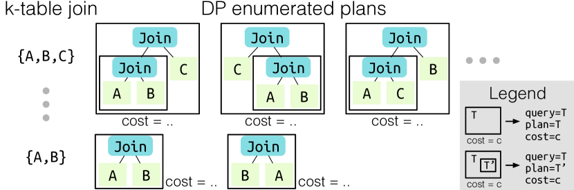
Figure 2. Simulation data collection and augmentation. For each $k$-table join in DP, Balsa collects and augments all its enumerated plans. Each bordered box yields a collected data point (see legend).

Enumerating plans using dynamic programming. For each query in Balsa’s training workload, we run the classical Selinger (Selinger et al., 1979) bottom-up DP with a bushy plan space. It starts by enumerating the best plans for all valid 2-table joins, composed out of base table scans, then enumerating 3-table joins, etc. Each enumerated plan $T$ will get a cost estimate $C$ from the cost model, generating a data point (query=$T$, plan=$T$, overall cost=$C$), where query=$T$ denotes the original query restricted to the tables/filters of $T$. This data point undergoes a data augmentation procedure, described below, to yield a list of training data points to be added into $\mathcal{D}_{\text{sim}}$.

The data collection is high-throughput: data is generated from all enumerated plans, not just from the set of optimal plans in the final DP results. This means that some suboptimal plans (under the cost model) are included, which increase data variety and aid learning. Figure 2 illustrates the data collection procedure.

However, DP’s runtime may become too large for queries joining many tables. Hence we skip collecting data from queries with $\geq n$ tables (we set $n=12$). Alternative strategies can also be applied. For example, DQ proposes a partial DP scheme where the first $j$ levels of DP are run and the rest of the levels are planned greedily.

Data augmentation. Balsa employs a data augmentation technique proposed by DQ, where multiple data points are generated from a single enumerated plan. Specifically, given a (query=$T$, plan=$T$, overall cost=$C$), each subplan $T^{\prime}$ of $T$ will yield a distinct data point with the same “overall query” $T$ and the same cost: $\{\textsf{(query=$T$, plan=$T^{\prime}$, overall cost=$C$)}:\forall T^{\prime}\subseteq T\}$. This technique significantly enriches the dataset $\mathcal{D}_{\text{sim}}$ in quantity and variety.

Interpretation. In RL terms, the augmentation reflects that all states (the subplans) in a trajectory (the overall query/final plan) share the same return, because intermediate rewards are defined to be 0 and terminal rewards are the negative costs of final plans.

3.3. Discussion

We found simulation learning to be highly effective. At the start of §3, we performed a simple experiment illustrating an up to $79\times$ gap between randomly initialized (i.e., no bootstrapping) agents and an expert optimizer. Now, with simulation bootstrapping, agents significantly shorten this gap to only $5.8\times$ slower than the expert at max—all without performing any real execution.

Cardinality estimator. The simulator needs a cardinality estimator. As mentioned in §1, we pick PostgreSQL’s estimator for its simplicity (per-column histograms; heuristically assumes independence for joins; “magic constants” for complex filters) (Leis et al., 2015). Balsa does not learn from PostgreSQL’s optimizer (costs or plans).

We use an existing, textbook-style estimator for convenience, not to rely on it for good performance. In fact, most of Balsa’s quality improvements are learned after the simulation stage (§8.2, §10).

Alternative cost models. While Balsa advocates for a minimal simulator, more prior knowledge can be plugged in by the user, if desired. Other cost models may include progressively more physical operator knowledge (e.g., the $C_{mm}$ cost model (Leis et al., 2015) for in-memory settings). New query engines optimizing for different objectives (e.g., lower memory footprint) may either bootstrap Balsa with $C_{out}$ (its fewer-tuples-are-better principle generally applies), or develop another minimal cost model tailored to the objective.

4. Learning from Real Execution

Simulation learning imparts basic knowledge to the agent. But no simulators can perfectly reflect the nuances of the real execution environment. Therefore, we fine-tune the agent through query executions in the real environment.

4.1. Reinforcement Learning of the Value Function

Balsa learns the real-execution value network, $V_{\text{real}}(\textsf{query},\textsf{plan})\rightarrow\textsf{overall latency}$, using reinforcement learning. The basic idea is that the agent iteratively uses its current value network to optimize queries and runs them, then uses the latency feedback to improve itself. As this feedback loop runs, more execution data is collected, and the agent’s $V_{\text{real}}$ becomes better at generating good plans.

Concretely, we start with $V_{\text{real}}$ initialized from $V_{\text{sim}}$ and an empty real-execution dataset, $\mathcal{D}_{\text{real}}=\emptyset$. Each iteration of learning consists of an execute and an update phase.

Execute. The agent uses the current $V_{\text{real}}$ to optimize each training query $q$, producing an execution plan $p$. (Planning will be described in §4.2.) Each plan is executed on the target engine with its latency $l$ measured. This results in one data point, (query=$q$, plan=$p$, overall latency=$l$), which then undergoes the same subplan data augmentation discussed in §3.2 to yield a list of data points:

$$\mathcal{D}_{\text{real}}\mathrel{{+}{=}}\{(\textsf{query}=q,\textsf{plan}=p^{\prime},\textsf{overall latency}=l):\forall p^{\prime}\subseteq p\}$$

Update. Balsa uses the collected data to improve its $V_{\text{real}}$. We perform stochastic gradient descent (SGD) with an L2 loss between predicted and true latencies. Thus, mispredictions are corrected and good predictions are reinforced. Data points $(q,p,l)$ are sampled from $\mathcal{D}_{\text{real}}$. However, model outputs $V_{\text{real}}(q,p)$ are updated not towards $l$, but towards the best latency obtained so far of query $q$ that involves subplan $p$—a previously proposed technique (Marcus et al., 2019). The latency label correction is motivated as follows. Consider query $q$ joining tables $A,B,C,D$. Subplan $p=$ Join$(A,B)$ may have appeared in two executions, one with $C$ joined next and one with $D$ joined next. They may have wildly different latencies, say 1 vs. 100 seconds. As we wish to minimize latency, we define the lower latency $l=1$ as the value of subplan $p$, because $p$ could have made $q$ run this fast. The best latencies so far are calculated from the entire $\mathcal{D}_{\text{real}}$.

Thus, data collection and value function improvement alternate. The algorithm can be thought of as either value iteration (Sutton and Barto, 2018) or expert iteration (Anthony et al., 2017), and variants of it have been recently applied in prior work in query optimization (Marcus et al., 2019) (which, different from Balsa’s updates, resets and retrains the value network across iterations) , theorem proving (Polu and Sutskever, 2020), and compute schedule optimization (Adams et al., 2019).

On-policy learning. Balsa employs a novel optimization on top of the algorithm above by using on-policy learning. Updates to $V_{\text{real}}$ are performed only on the data points generated by the current $V_{\text{real}}$. In other words, SGD is performed on data points $(q,p,\_)$ sampled from the most recent iteration of the dataset, $\mathcal{D}_{\text{real}}$, but not from its entirety. The latter would yield data from many iterations ago and is hence off-policy. Label correction still utilizes the entire dataset.

Intuitively, the most recent data points generally are the most surprising to the agent and have faster latency labels, so it should be beneficial to focus on them. Indeed, we find on-policy learning to significantly accelerate learning, by reducing the number of SGD steps per iteration, and improve the plan variety and performance of Balsa (§8.3.4). On-policy learning makes Balsa’s training more than $9.6\times$ faster when compared to Neo (Marcus et al., 2019), a prior state-of-the-art method, which employs a full retraining scheme instead (§8.4). We hypothesize that this technique may also improve other applications of value functions that predict runtimes.

4.2. Plan Search

With the learned value network, Balsa uses a simple (best-first) beam search to produce execution plans for a given query.

Beam search operates on search states, each a set of partial plans for the query. The search starts with a root state that contains all tables (scans) in the query. A beam of size $b$ stores search states to be expanded, sorted by their predicted latencies. At each step, the best search state is popped from the beam, and all available actions are applied to produce children states. Each action joins two eligible plans in the current state with a physical join operator assigned, as well as assigning scan operators if either side is a table. As a search state is a set of partial plans (joined relations and non-joined tables), applying actions to it will lead to at least one complete plan.

Then, all resulting children states are scored by the value network $V_{\text{real}}$ and added to the beam, which keeps the top $b$ states only. In this way, the learned value network guides the search to focus on the more promising regions of the plan space. Beam search terminates when $k$ complete plans are found. Balsa uses $b=20$ and $k=10$.

Top-$k$ plans and exploration. Beam search is not guaranteed to return globally optimal plans, and better plans may be found later in the search. We thus continue searching until $k$ complete plans are found. At test time, the best plan out of this list is emitted.

Interestingly, at training time, obtaining a list of plans enables a simple exploration technique on top. We treat all of these plans as having reasonable optimality—so that it should be safe to explore among them—and prioritize choosing the unseen plans as beam search outputs. This technique is discussed in §5.

4.3. Safe Execution via Timeouts

A unique challenge in query optimization is the proliferation of expensive plans in a vast search space, even when fast plans exist. When Balsa learns by trial and error from real executions, it can encounter long-running plans with unacceptably high latencies.

Balsa addresses this challenge by applying timeouts, a classical idea in distributed systems. Since training proceeds in iterations, earlier execution runtimes of the same training workload are known and can be used to bound future iterations.

Key to this mechanism is how to pick the initial timeout. Fortunately, simulation learning allows us to assume that when the real execution starts, the first ever plans produced for a set of training queries have reasonable (albeit suboptimal) latencies.

Timeout policy. During iteration 0’s execute phase (just after simulation learning), the plans are allowed to finish execution in their entirety—simulation learning is assumed to yield a non-disastrous starting point. Let the maximum per-query runtime recorded be $T$.

For iteration $i>0$, a timeout of $S\times T$ is applied for all agent-produced plans, where $S$ is a “slack factor”. By definition of $T$, for any training query there exists a plan that can finish execution in time $T$. The slack’s purpose is to give some extra room and account for runtime variance (Balsa uses $S=2$).

If a plan has been executing longer than the current timeout, it is terminated early, since it would be slower than earlier found plans for the same query anyway. It gets assigned a large label instead of its true, unknown latency. Such large labels serve to discourage and steer the agent away from similar plans in future iterations.

Timeouts are progressively tightened. If an iteration finishes with a maximum per-query runtime $T^{\prime}<T$, then the next iteration’s timeout is tightened to $S\times T^{\prime}$. This progression ensures that the timeout is neither too small, which prevents progress, nor too large, which wastes efforts. It generates an implicit learning curriculum for the agent with just-about-right difficulties.

In sum, we found the timeout mechanism to significantly accelerate learning. It bounds the runtime of each iteration’s execute phase and eliminates unexpected stalls, thereby achieving safe execution.

5. Safe Exploration in Real Execution

While an RL agent exploits its past experience for good performance, it must also explore new experience to escape local minima. To achieve this, an exploration strategy can be used.

However, the abundance of slow plans, a unique characteristic of query optimization, additionally requires safe exploration, i.e., disastrous plans be avoided. Random plans sampled from the search space are slow (Leis et al., 2015), and choosing to explore them would again stall learning. In our early experiments, a basic $\epsilon$-greedy strategy (for each training query, with a small $\epsilon$ probability a random plan is sampled, a la QuickPick (Waas and Pellenkoft, 2000)) often selected inferior plans that led to timeouts, slowing down the discovery of better plans and learning.

To achieve safe exploration, Balsa proposes a simple count-based exploration technique. In essence, this family of methods encourages an agent to explore a less-visited state or execute a less-chosen action. We instantiate this principle in the following way.

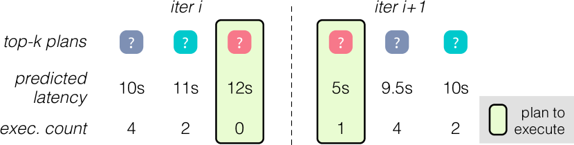
Figure 3. Safe exploration. For a training query, Balsa prioritizes running the unseen plans of the top-$k$ plans from tree search (exploration). If all seen, the predicted-best plan is chosen (exploitation).

Count-based exploration for beam search. Our goal is to provide a “trust region” of reasonable plans for the agent to explore. To do so, beam search is asked to return top-$k$ plans, sorted by ascending predicted latencies, rather than the single best plan found. Instead of executing the best plan (i.e., with the lowest predicted latency), we execute the best unseen plan of this list. If all top-$k$ plans have been previously executed—indicating sufficient exploration—Balsa resorts to exploitation by executing the predicted-cheapest plan. The visit counts of plans are cached by a hash table, which adds low overheads, as past executions are already stored in $\mathcal{D}_{\text{real}}$. Figure 3 illustrates this technique using example statistics ($k=3$).

Intuitively, all of the top-$k$ plans are probably good (since they are produced by value network-guided beam search), so they should not be chosen strictly by their predicted latencies (which are imperfect estimates). Therefore, executing novel, unseen plans in this “trust region” is both safe and exploratory.

6. Diversified Experiences

For learned query optimizers, robustly optimizing unseen queries is essential. To further enhance Balsa’s generalization performance, we introduce a simple method, diversified experiences.

Problem: mode diversity. As a value network is used to guide plan search, an agent tends to only experience plans preferred by its value network, and may gradually converge to plans with similar characteristics, or a “mode” (Weisstein, [n. d.]). For example, if hash and loop joins are equally effective for a workload, an agent may learn to heavily use hash joins, while another may prefer loop joins. Either agent can output good plans, as both operators are effective, but they may lack the knowledge about plans that prefer alternative operators or shapes. (While exploration increases plan variety, the new plans are still relatively confined to a single agent’s mode.) Low mode diversity can hinder an agent’s generalization to highly distinct, unseen queries that require unfamiliar modes to be optimized well.

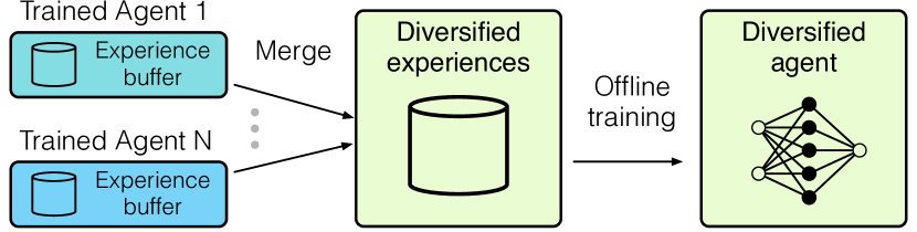
Figure 4. Diversified experiences. A more robust agent is produced by retraining on the experiences collected from different agents.

Diversified experiences. To enhance generalization, we propose simply merging the experiences ($\mathcal{D}_{\text{real}}$) collected by several independently trained agents (with different random seeds), and retraining a new agent on top without any real execution. Figure 4 illustrates this process. Our insight is that this diversified experience covers multiple modes. Thus, training on it produces a more robust value network that generalizes better.

Table 1. Diversifying experiences: number of data collection agents vs. number of unique plans after merging. Agents have highly diverse experiences. Trained on 113 JOB queries (details in §8.1).

Num. Agents	1	4	8
Num. Unique Plans	27K (1$\times$)	102K (3.8$\times$)	197K (7.3$\times$)

Table 1 confirms this insight: the number of unique plans grows almost linearly as the number of agents, showing that the plans experienced by different agents are indeed highly diverse. We find this simple method effective (§8.5), offering a way to trade more compute, when available, for better performance.

7. Balsa Implementation

In this section we describe Balsa’s detailed training setup. At a high level, to operate Balsa on a new engine it needs the following:

• An execution environment (executes plans; support for timeouts).

• Definition of the search space (the set of query operators and the rules to compose them).

Optimizations. We optimize training by parallel data collection, plan caching, and pipelining. Query executions are dispatched to a pool of identical virtual machines each running an instance of the target database, using Ray (Moritz et al., 2018). Each VM runs one query at a time to prevent interference. A plan cache is used so that reissued plans have their prior runtimes quickly looked up and can skip re-execution. Planning and remote query execution in each iteration are pipelined (Figure 5): as soon as tree search (run by the main agent thread) finishes planning a training query, the output plan is sent for remote execution, and then planning for the next query starts. The two stages thus overlap. The agent waits for all plans to finish before performing value network updates.

Value network details. The value networks, $V_{\text{sim}}$ and $V_{\text{real}}$, are implemented as simple tree convolution networks (Marcus et al., 2019) (0.7M parameters, or 2.9MB). We also experimented with implementing them using a Transformer (Vaswani et al., 2017) early on; this was found to be similarly effective but had higher computational costs. When training or updating the value networks, we sample 10% of experience data as a validation set for early stopping. The inputs to the value network, query and plan, are encoded as follows. Each plan has the same encoding as Neo (Marcus et al., 2019). A query is featurized as a vector $\textsf{[}\textsf{table}\rightarrow\textsf{selectivity}\textsf{]}$ where each slot corresponds to a table and holds its estimated selectivity (§3.3). Absent tables’ slots are filled with zeros. This encoding is simpler than both Neo and DQ (Krishnan et al., 2018).

Figure 5. Pipelining agent planning and remote query execution.

8. Evaluation

We conduct an in-depth evaluation of Balsa. Our key findings are:

• Learning by trial and error, Balsa generates better execution plans that run up to 2.1–2.8$\times$ faster in workload runtime than two expert optimizers, PostgreSQL and “CommDB” (§8.2).

• Balsa takes a few hours to surpass the experts and a few more hours to reach peak performance on the tested workloads (§8.2).

• Balsa outperforms learning from expert demonstrations (Marcus et al., 2019), a prior state-of-the-art approach, despite not learning from an expert optimizer (§8.4). We also identify poor generalization as a potential failure mode in this prior method.

• Diversified experiences significantly enhance generalization, including to queries with highly distinct join templates (§8.5).

• Balsa learns novel preferences of operators and plan shapes (§8.6).

Additionally, we conduct detailed ablation studies to understand the effect of Balsa’s design choices in §8.3.

8.1. Experimental Setup

We use the following workloads, in each of which Balsa is trained on a set of training queries and tested on a set of unseen queries:

Join Order Benchmark (JOB) contains 113 analytical queries designed by Leis et al. (Leis et al., 2015) to stress test query optimizers over a real-world dataset from the Internet Movie Database. The queries involve complex joins and predicates, ranging from 3-16 joins, averaging 8 joins per query. We benchmark against two train-test splits, each with 94 training and 19 test queries:

• Random Split (denoted as “JOB”): a randomly sampled split.

• Slow Split (denoted as “JOB Slow”): the test set consists of the 19 slowest-running queries when planned by an expert optimizer.

Random Split tests an average situation, while Slow Split evaluates when the test queries run maximally slower than the train queries.

TPC-H is a standard analytical benchmark where data and queries are generated from uniform distributions. We use a scale factor of 10. We use 70 queries for training and 10 queries as the test set.

Expert baselines and engines. We compare with the optimizers of two mature expert systems: PostgreSQL (12.5; open-source) and CommDB (a leading commercial DBMS; anonymized (Read, 2006)). For each expert, we compare Balsa’s plans with its optimizer’s plans executed on that same engine. Balsa’s plans are injected by hints (Development and Team, 2020).

We use Microsoft Azure VMs with 8 cores, 64GB RAM, and SSDs. Training is done on a NVIDIA Tesla M60 GPU. We configure PostgreSQL with 32GB shared buffers and cache size, 4GB work memory, and GEQO disabled—settings similar to Leis et al. (Leis et al., 2015). We optimize CommDB extensively by following its tuning guides.

Balsa is trained for 500 iterations on the JOB workloads and 100 iterations on TPC-H due to its smaller search space. Balsa uses all components and default values discussed in prior sections.

Expert performance. We follow the guidance in Leis et al. (Leis et al., 2015) to create all primary and foreign key indexes to make our baselines run JOB much faster than that of prior work (Marcus et al., 2019; Trummer et al., 2019). This also makes the search space more complex and challenging.

Metrics. We repeat each experiment 8 times and report the median metric, unless specified otherwise. In train/test curves, we show the entire min/max ranges in shaded areas. Workload runtime is defined as the sum of per-query latencies. When reporting normalized runtimes, they are calculated with respect to the expert’s runtimes.

8.2. Balsa Performance

We begin with end-to-end results, answering the following:

• What is the performance of Balsa on training and test queries?

• How many hours (and executions) does Balsa need to surpass expert performance and reach its peak performance, respectively?

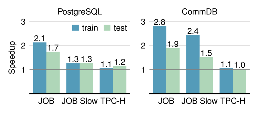
Figure 6. Balsa’s performance on PostgreSQL (left) and CommDB (right): workload speedups achieved by Balsa plans over plans from the respective expert optimizer. Each bar is the median of 8 runs.

Performance. Figure 6 summarizes Balsa’s overall performance. On all workloads, Balsa is able to start from a minimal cost model and learn to surpass the expert optimizers by a sizable margin.

On PostgreSQL, Balsa achieves a $2.1\times$ training-set speedup on JOB, $1.3\times$ on JOB Slow, and $1.1\times$ on TPC-H. While speedups on test sets slightly trail behind the training set speedups, Balsa can still produce faster execution plans than the expert (e.g., $1.7\times$ faster on JOB). This shows that Balsa can generalize to unseen queries.

Balsa also outperforms CommDB’s optimizer. The speedups are higher—1.1–2.8$\times$ for train and 1.0–1.9$\times$ for test sets—because CommDB allows a much smaller search space than PostgreSQL by not exposing bushy hints. (We estimate it to be 1000$\times$ smaller for an average-sized JOB query, counting plan shapes and operators.) Balsa thus explores the smaller search space more comprehensively.

Runtime of simulation learning. Table 2 shows simulation is data-rich and takes dozens of minutes. As it is a small fraction of real execution learning’s duration, we focus on the latter next.

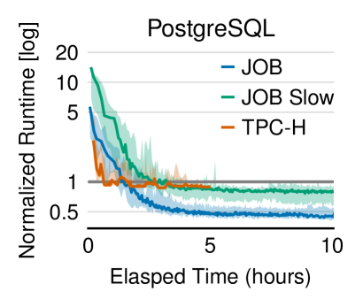
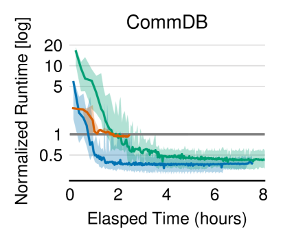
(a) Wall-clock efficiency

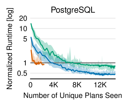
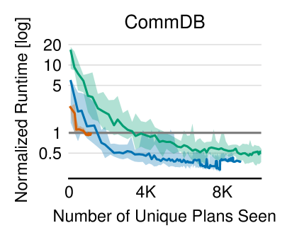
(b) Data efficiency

Figure 7. Learning efficiency of Balsa. Normalized runtime of training queries (log scale) vs. (a) elapsed time and (b) number of executed plans.

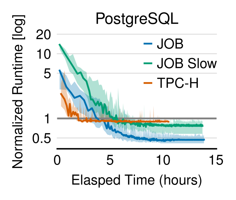
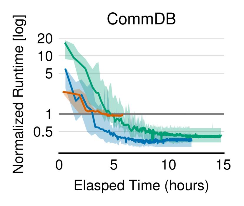
Figure 8. Wall-clock efficiency, non-parallel training mode.

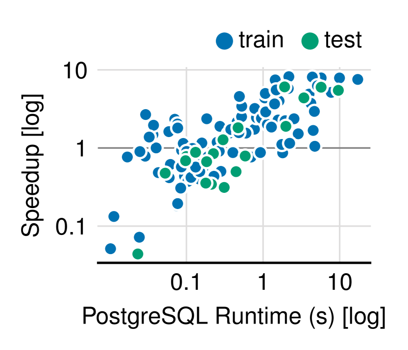
(a) JOB

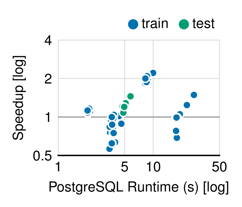
(b) TPC-H

Figure 9. Breakdown of Balsa’s per-query speedups. Speedup of each query (log scale) vs. PostgreSQL expert runtime (log scale).

Table 2. Simulation learning efficiency: sizes of simulation datasets, time to collect data (in minutes), and time to train. Train times differ due to early stopping. Means $\pm$ standard deviations are shown.

Workload	Size	Collection time (min.)	Train time (min.)
JOB	516K	$6.8\pm 0.1$	$24\pm 8$
JOB Slow	551K	$7.6\pm 0.1$	$28\pm 10$
TPC-H	12K	$1.1\pm 0.01$	$1.0\pm 0.2$

Learning efficiency. Figure 7 shows the training performance of Balsa as a function of elapsed time and the number of distinct query plans executed. (The latter is called data/sample efficiency in RL terms, as each execution is an interaction with the environment.)

Wall-clock efficiency. 7(a) shows Balsa’s wall-clock efficiency during the real execution stage. Balsa starts off several times slower than the experts—this is the performance after bootstrapping from a simple simulator. With just a few hours of learning, Balsa matches the experts’ performance (on PostgreSQL: 1.4 hours for JOB, 2.5 hours for JOB Slow, 1.5 hours for TPC-H; ${\sim}0.5$ hours faster on CommDB due to its smaller search space). Balsa continues to improve and reaches its peak performance after around 4–5 hours. TPC-H has less room for optimization—it has much fewer joins—so Balsa converges faster.

Data efficiency. 7(b) shows data efficiency curves. It takes a few thousand executions to reach the experts’ performance (on PostgreSQL: 3.2K for JOB, 7.4K for JOB Slow, 0.7K for TPC-H; on CommDB, ${\sim}60\%$ fewer plans are needed). The number of query plans required is higher for workloads where the agent starts with slower performance. Therefore, experiencing more plans helps Balsa improve performance by a greater amount.

Non-parallel training wall-clock. Throughout our evaluation, including the discussions above and Figure 7, we configure Balsa to use a few query execution nodes per run (average: 2.5 nodes/run) to speed up training. For completeness, Figure 8 shows non-parallel training times where each run uses one execution node. In all cases, peak performance is reached within single-digit hours, a comfortable “nightly maintenance” range. The time to match the experts is at most 3 hours slower than that for the parallel mode.

Sources of speedup. Figure 9 shows Balsa’s per-query speedups over PostgreSQL plans. For JOB, Balsa produces better query plans for most queries in both training and testing. Notably, Balsa considerably speeds up the slowest queries. Slowdowns mostly occur in the queries that are inherently fast to execute, and hence minimally affect the overall runtime. A similar trend holds for TPC-H.

Summary. Balsa can bootstrap from a minimal cost model and learn to surpass both an open-source and a commercial expert optimizer. Balsa is efficient to train, needing a few hours to match the experts and thousands of plans to reach its peak performance.

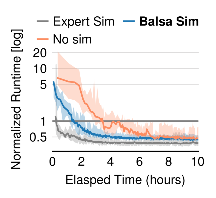
(a) Training performance

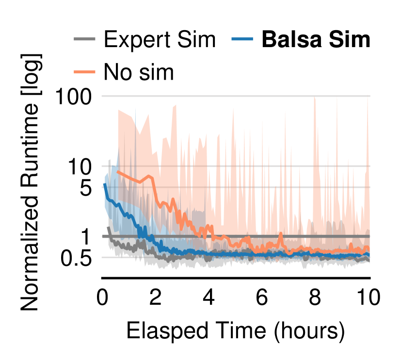
(b) Test performance

Figure 10. Impact of the initial simulator. (a) Better simulators accelerate learning. (b) Simulation is essential for generalization.

8.3. Analysis of Design Choices

Next, we analyze the design choices of each major component in Balsa: (1) the initial simulator, (2) the timeout mechanism, (3) exploration strategies, (4) the training scheme, and (5) beam search. In summary, we found all components to positively contribute to Balsa’s performance and generalization.

In each experiment, we change one component at a time and hold all other configurations fixed at default values. We then measure each variant’s performance on the JOB (random split) workload on PostgreSQL. Default choices are highlighted in bold in each figure.

8.3.1. Impact of the initial simulator.

Balsa bootstraps from a minimal simulator. We can consider two alternatives that differ the most from this choice in terms of the amount of prior knowledge:

• Expert Simulator: the cost model from an expert optimizer, PostgreSQL, which has sophisticated modeling of all physical operators and captures the nuances of its execution engine. (Note that this variant means Balsa uses this cost model as the simulator; it does not represent PostgreSQL’s own plans.)

• Balsa Simulator (§3; $C_{out}$): a minimal cost model that sums up the estimated result sizes of all operators. It has no knowledge about physical operators or the execution engine.

• No simulator: skip bootstrapping altogether and initialize the agent from random weights.

Figure 10 shows the simulator’s impact. We make four observations:

First, simulators with more prior knowledge shorten the time to reach expert performance on training queries (10(a)). Balsa with an expert simulator needs only ${\sim}0.3$ hours of learning to match the expert. Balsa’s default simple simulator takes ${\sim}1.4$ hours to match, while agents without simulation learning take ${\sim}3.8$ hours.

Second, more prior knowledge also leads to slightly better final performance at the end of training (10(a)). The gap, however, is relatively small. Agents using a minimal simulator mostly catch up with those using an expert simulator.

Third, it is a pleasant surprise that the agents without simulation (“No sim”) can finish training. This is enabled by the use of timeouts and safe exploration, which keep the bulk of the learning safe.

Fourth, simulation is essential for generalization. Agents without simulation learning can fail at test time (note the high variance of “No sim” in 10(b)). The unstable performance on test queries occurs despite good training performance, rendering this choice impractical. The instability is caused by randomly initialized agents overfitting the experience collected during the real execution phase, which is limited in quantity (${\sim}700$ subplans per iteration, so it takes at least ${\sim}700$ iterations to catch up to the 0.5M-plan simulation dataset, assuming each iteration’s data is unique).

In summary, bootstrapping from a minimal simulator gives good train and test time performance. Since new execution engines may not have an expert-developed cost model, this approach has the additional benefit of potentially generalizing to new systems and alleviating the human development cost.

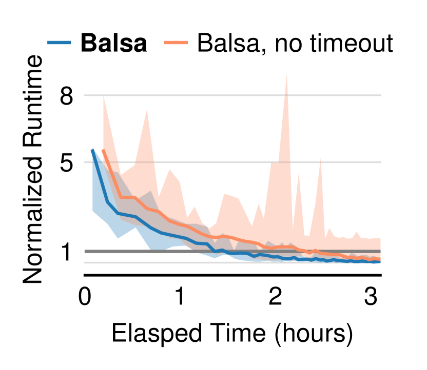
(a) Initial training performance

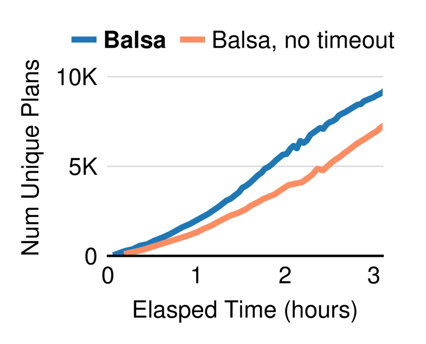
(b) Number of executed plans

Figure 11. Impact of the timeout mechanism. (a) Timeouts accelerate learning and prevent spikes. (b) With the same wall-clock time, agents with timeouts execute more plans, improving plan variety.

8.3.2. Impact of the timeout mechanism.

We study the impact of timeouts (§4.3), a mechanism critical for real execution learning:

• Timeout: early-terminate query plans that have been executing for longer than the current iteration’s timeout.

• No timeout: the mechanism is turned off.

With timeouts, agents are expected to save wall-clock time on unpromising plans and potentially learn faster.

Results are presented in Figure 11. Timeout agents reach expert performance about 35% faster than no-timeout agents (11(a)). While both choices lead to similar final performance, there is a pronounced difference in the initial phase of learning. Agents without timeouts may execute expensive query plans, leading to significant spikes. Such regressions are unpredictable: they can happen after the no-timeout agents reaching expert performance.

In contrast, agents achieve safe execution when timeout is enabled. The early-terminated plans “nudge” the agents in a different direction to look for more promising plans. 11(b) shows how the saved time is more judiciously spent: with the same wall-clock time, agents with timeouts run more plans, speeding up learning.

Overall, these results show that the timeout mechanism accelerates learning and improves Balsa’s plan variety.

8.3.3. Impact of exploration.

Exploration exposes RL agents to diverse states, boosting performance and generalization. We compare:

• Count-based exploration (§5): Balsa’s safe exploration method, which chooses the best unseen plan from beam search outputs.

• $\epsilon$-greedy beam search: at each step of the search, with a small probability $\epsilon$ the beam is “collapsed” into one state, discarding the rest. The search continues as usual. We chose $\epsilon$ such that about 10% of training queries have random joins injected.

• No exploration: no exploration algorithms are used.

12(a) shows that agents with count-based safe exploration generalize to test queries much better than the other two variants. The better generalization is a result of the higher number of distinct plans experienced (12(b)). Training performance is omitted for space reasons, where count-based is around 8% and 14% faster than no-exploration and $\epsilon$-greedy beam at convergence, respectively.

Interestingly, although $\epsilon$-greedy beam search has similar plan diversity to count-based, it is less stable. This is because it contains random joins, which may only lead to low-quality complete plans even when a value network is used to guide the remaining search.

In summary, these results show that safe exploration is non-trivial, and Balsa’s count-based method is both simple and effective.

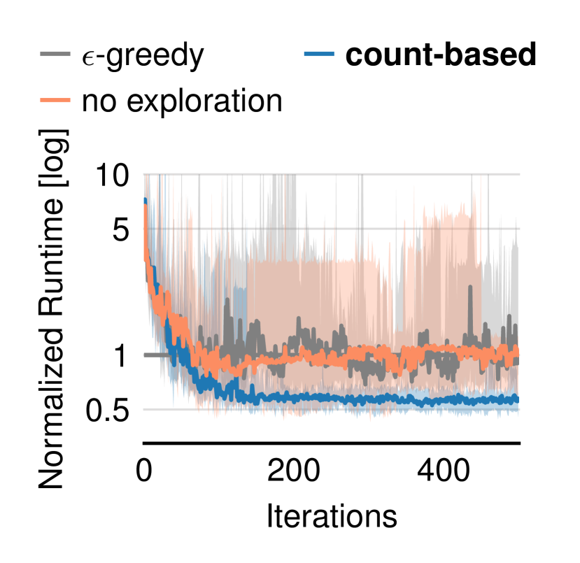
(a) Test performance

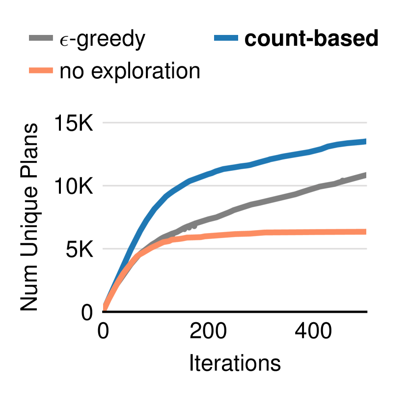
(b) Number of unique plans seen

Figure 12. Impact of exploration. Balsa’s count-based safe exploration improves generalization to unseen test queries.

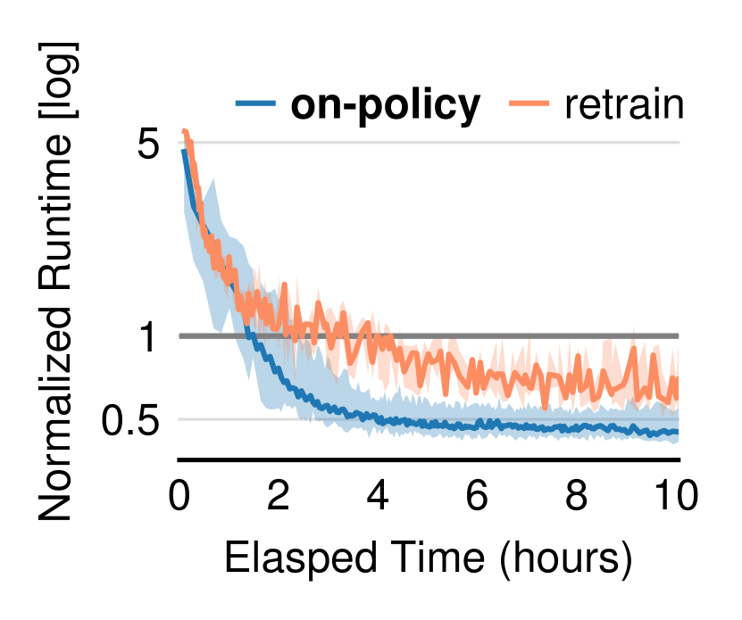
(a) Training performance

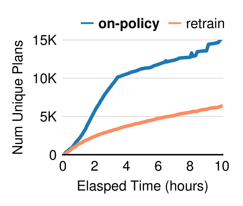
(b) Number of unique plans seen

Figure 13. Impact of the training scheme. (a) On-policy learning accelerates training. (b) Time saved is used towards more exploration.

8.3.4. Impact of the training scheme.

We compare Balsa’s on-policy learning to a full retrain scheme used by prior work, Neo (Marcus et al., 2019):

• On-policy learning (§4.1): Balsa’s training scheme which uses the latest iteration’s data to update $V_{\text{real}}$.

• Retrain: re-initialize $V_{\text{real}}$ and retrain on the entire experience ($\mathcal{D}_{\text{real}}$) at every iteration. Last iteration’s $V_{\text{real}}$ is discarded.

On-policy learning significantly accelerates training, reaching the expert’s performance 2.1$\times$ faster than retrain agents (13(a)). Its lead is consistent throughout training. The faster learning is due to on-policy saving time by updating $V_{\text{real}}$ on a constant-size dataset, rather than retraining it on an increasingly larger dataset. The time saved is used towards exploration, i.e., executing more unique plans (13(b)). Better exploration thus further accelerates learning. On-policy has slightly higher variance due to performing SGD on much less data. However, the slowest on-policy agent (the upper edge of the shading) is still mostly faster than retrain agents.

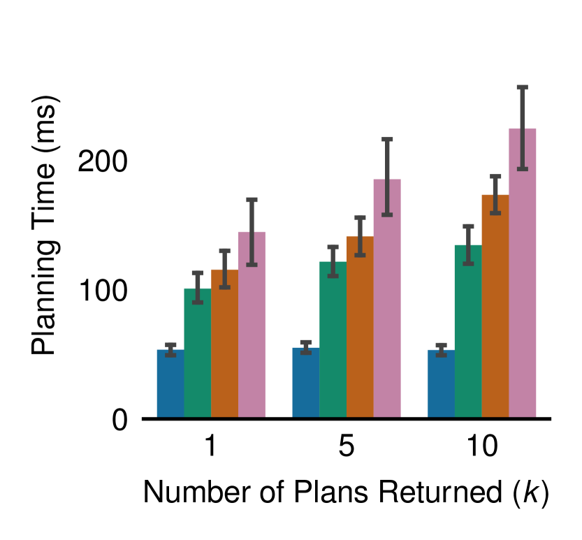
(a) Per-query planning time

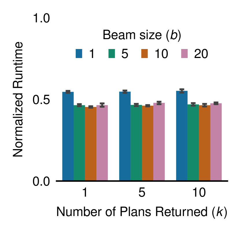
(b) Workload runtime

Figure 14. Impact of search parameters on planning time and performance on JOB test set. Means and standard deviations are shown.

8.3.5. Impact of planning time.

Balsa performs beam search with beam size $b$ using the value network to generate $k$ complete query plans, and then picks the best plan to execute (during training, the best unexplored plan is picked). Figure 14 studies Balsa’s planning time and performance of the JOB test queries using various combinations of $b$ and $k$ on a trained checkpoint.

For all settings, the mean per-query planning time is below 250ms. The planner is implemented in Python and thus leaves room for optimization. Using $b=1$ (where beam search degenerates into greedy search) slightly hurts performance; all other settings produce plans with similar runtime. Hence, Balsa’s performance is insensitive to these parameters, and we can flexibly reduce planning time for deployment by using lower values (e.g., $b=5,k=1$ speeds up planning time by $2\times$ with no performance drop). We use $b=20,k=10$ during training as larger values can help exploration.

8.4. Comparison with Learning from Expert Demonstrations

We compare Balsa with Neo (Marcus et al., 2019), a recently proposed learned optimizer that relies on PostgreSQL-generated plans—i.e., learning from expert demonstrations. This experiment uses the same setup as §8.3 (JOB workload on PostgreSQL). As Neo is not open source, we implement our best-effort reproduction, denoted as “Neo-impl”. We make both approaches use identical modeling choices (e.g., architecture, featurizations, beam search), and turn off Balsa’s algorithmic components for Neo-impl (bootstrapping from simulation; on-policy learning; exploration; timeout mechanism). One notable difference is that Neo completely resets its model to random weights in each iteration and retrains it on the entire collected experience.

15(a) shows training performance. At initialization, Balsa is 5$\times$ faster than Neo-impl, since simulation learning provides a high state coverage (Table 2) as opposed to a limited number of expert demonstrations (one complete plan per query). Balsa remains stable throughout training, as it employs timeouts. Neo-impl experiences performance spikes (note the variance) as it has no mechanism to deal with disastrous plans. These regressions are unpredictable and can occur after hours of training. In terms of training efficiency, Neo-impl’s retraining scheme makes it progress increasingly slower as the amount of experience accumulates. Neo-impl spent about 25 hours to finish 100 iterations, whereas Balsa only spent 2.6 hours.

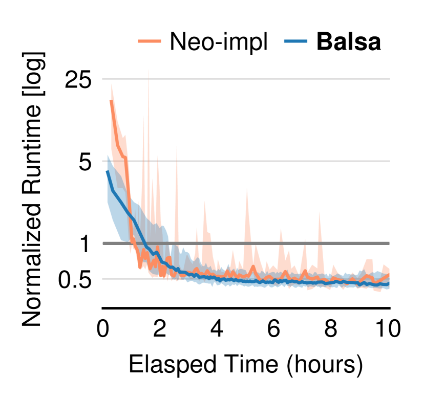
(a) Training performance

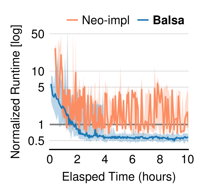
(b) Test performance

Figure 15. Comparison with learning from expert demonstrations.

Surprisingly, despite reaching a relatively stable training performance with 5 hours of learning, Neo-impl is still not robust enough to generalize to unseen test queries and suffers from high variance (15(b)). Its median workload runtime fluctuates between 1–5$\times$ slower than the expert and its maximum is up to $10\times$ worse. This failure mode may prohibit this approach from producing reliable models for practical deployment.

In contrast, Balsa is much more robust. Balsa consistently generates faster plans than the expert for unseen queries, with a 2$\times$ maximum speedup. Balsa’s better generalization is due to a broader state coverage offered by simulation, on-policy learning, and safe exploration (see Figures 12 and 13).

In sum, Balsa learns faster, achieves safe execution, generalizes better due to simulation and better exploration, while refuting the previously held belief that expert demonstrations are needed (Marcus et al., 2019).

8.4.1. Comparison with Bao

Bao (Marcus et al., 2021) is a related approach that assumes an expert optimizer is available. Like Neo, it requires expert demonstrations to train its model. Bao learns to provide a set of hints (e.g., disable hash join) for each query, “steering” the expert optimizer to produce better plans. This is different from Balsa which learns to produce physical plans by itself. Nevertheless, we compare the performance of the query plans generated by Balsa with those by Bao on top of PostgreSQL.

We substantially optimize the Bao source code (bao, 2020) as follows. First, we turn on an optimization that bootstraps its model from PostgreSQL’s expert plans, rather than from a random state. Second, its paper specifies that it trains on the most recent $k=2000$ experiences, which we found led to highly unstable performance. We thus train Bao on all past experiences, stabilizing convergence.

Table 3. Balsa vs. Bao: speedups with respect to PostgreSQL.

	JOB, train	JOB, test	JOB Slow, train	JOB Slow, test
Balsa	$2.1\times$	$1.7\times$	$1.3\times$	$1.3\times$
Bao	$1.6\times$	$1.8\times$	$1.2\times$	$1.1\times$

Table 3 shows that Balsa generally matches or outperforms Bao. These results are not surprising: they confirm the finding in the Bao paper that a learned optimizer with higher degrees of freedom (action space) can outperform Bao in plan quality on stable workloads.

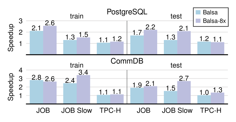
Figure 16. Enhancing generalization using diversified experiences.

8.5. Enhancing Generalization

Figure 6 already shows that Balsa can generalize to unseen test queries quite well, outperforming experts without ever seeing the test queries. Here, we study (i) the benefit of diversified experiences (§6), and (ii) generalizing to entirely distinct join templates/filters.

Diversified experiences. We build diversified experiences for all workloads/engines in Figure 6, by merging the data of each main experiment’s eight agents. We retrain a new agent on top, referred to as “Balsa-8x”; this process is repeated eight times to control for training variance. (Training is efficient as no query executions are performed.) Figure 16 shows the median performance: we observe that Balsa-8x improves speedups on both training and test queries in almost all cases, sometimes even by 60–80% (JOB Slow, test).

Improving training speedups is not surprising: a retrained agent can mix-and-match the best plans found by the base agents. Importantly, test queries see large speedups too without ever being executed (e.g., on both engines, both JOB splits now have $>2\times$ test speedups). This is because diversified experiences have highly diverse plans, so more generalizable value networks can be trained on top.

Queries with entirely new join templates. We further examine Balsa’s generalization to difficult unseen queries. First, we split JOB using 4 slowest templates (17, 16, 6, 19) as the test set (20 queries) and the rest as the train set. On this new split, Balsa achieves good train and test speedups (1.4$\times$, 1.5$\times$), further confirming its robustness.

Second, we evaluate on Extended JOB (Ext-JOB), a hard generalization workload (Marcus et al., 2019). It has 24 new queries on the same IMDb dataset, having 2–10 joins and averaging 5 joins per query. These queries are challenging and “out-of-distribution” since they contain entirely different join templates and predicates from the original JOB.

Figure 17(a) shows the test performance of Neo-Impl and Balsa on Ext-JOB with the entire 113 JOB queries as the training set. While Balsa is more stable than Neo-impl, neither surpasses the expert on the Ext-JOB test set (although they come close). This confirms that Ext-JOB is a highly challenging generalization workload.

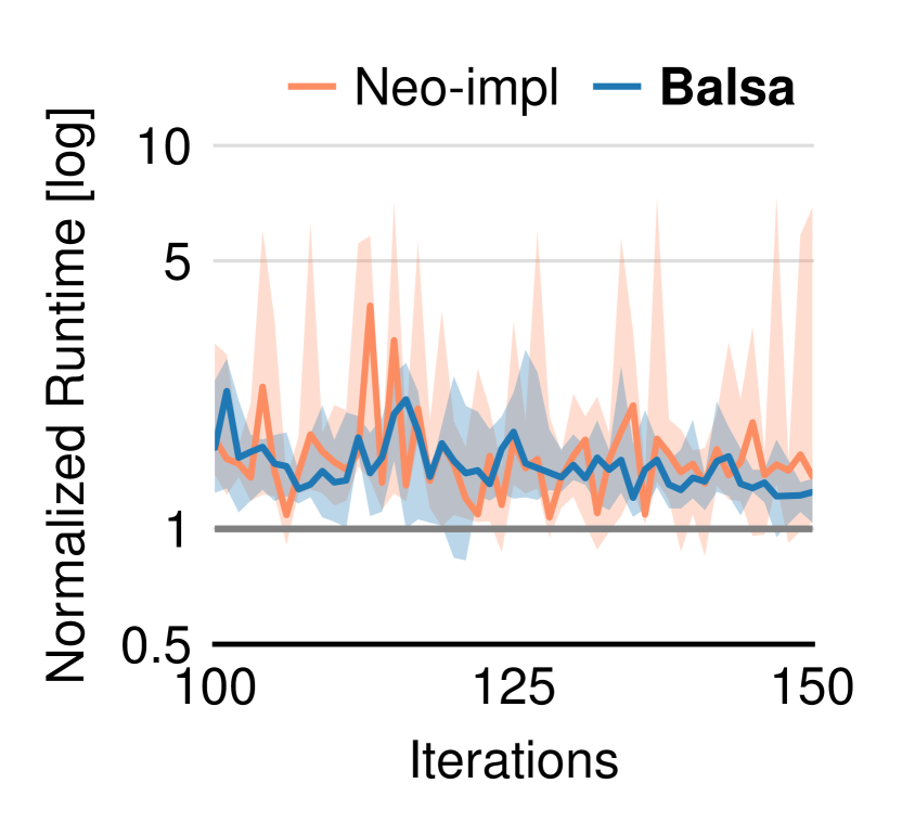
(a) Single-agent experiences

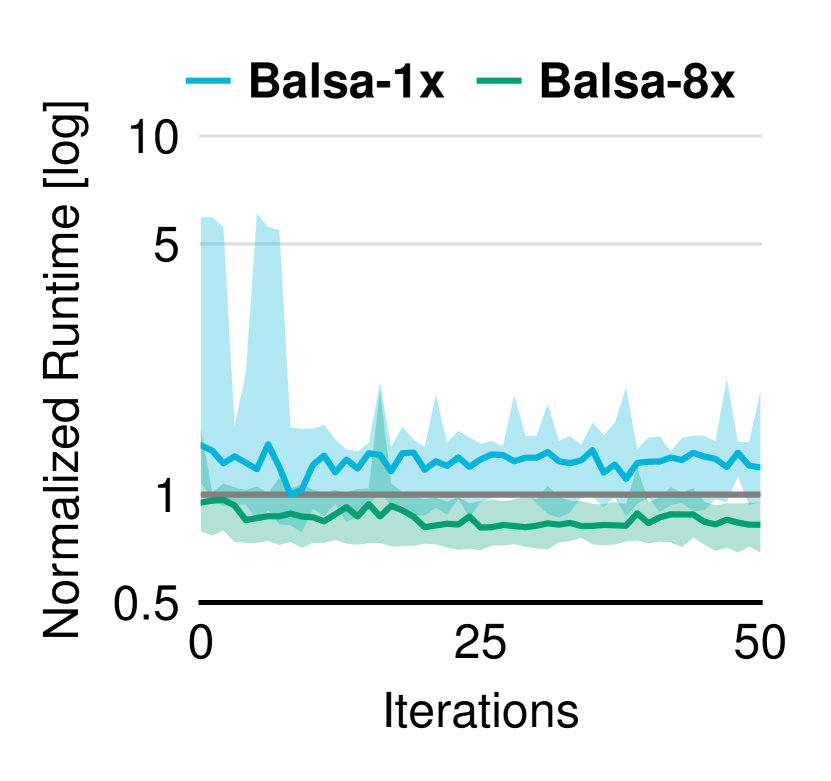
(b) Diversified experiences

Figure 17. Generalizing to highly distinct join templates: test performance on Ext-JOB, with JOB as the training set. On PostgreSQL.

Next, we compare Balsa-8x as described above, with Balsa-1x that retrains on only one agent’s data. Surprisingly, in iteration 0, Balsa-8x already matches the expert on the test set (17(b)). We then allow these agents to learn for 50 more iterations on the training set. Throughout the process, the agents never train on the Ext-JOB test queries. Balsa-8x reaches significantly better test set performance on Ext-JOB (20% faster than the expert) than Balsa-1x (which still fails to match the expert). The gain is also consistent. These results show that diversified experiences and further exploration are valuable strategies to improve generalization to out-of-distribution queries.

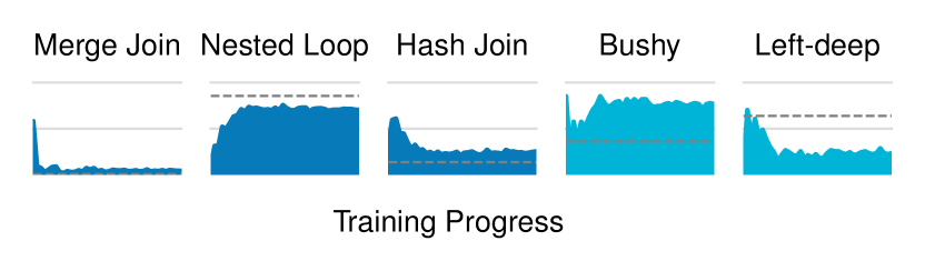
Figure 18. Balsa’s use of join operators (dark blue) and plan shapes (light blue) on JOB. Dashed lines are counts from PostgreSQL plans.

8.6. Behaviors Learned by Balsa

To gain intuition on the behaviors learned by Balsa, we visualize the operator and shape compositions of agent-produced plans over the course of training. Results are shown in Figure 18.

In early stages of training, Balsa quickly learns to reduce the use of operators and shapes that incur high runtimes in the current environment. For example, after 25 iterations, the use of merge joins is kept below 10%. Meanwhile, Balsa starts to prefer more efficient choices. Nested loop joins are preferred since a large portion (85% across iterations) are the efficient indexed variant.

Balsa’s preference is novel when compared to the expert, a difference especially pronounced in the plan shapes. This is due to the expert optimizer being one-size-fits-all, while Balsa learns to tailor to the given workload and hardware.

9. Related Work

Learned query optimizers. Balsa is most related to DQ (Krishnan et al., 2018) and Neo (Marcus et al., 2019). DQ offers the insight that the classical components of query optimization—cost estimation and plan enumeration—can be cast as long-term value estimation and planning. All three work follow this formulation by using a learned value network and plan search. Balsa also adopts DQ’s use of batched data collection on top of a cost model in our simulation learning. Unlike DQ, Balsa demonstrates fine-tuning entire workloads in real execution.

Neo requires learning from expert demonstrations (PostgreSQL plans) followed by fine-tuning. In contrast, Balsa does not learn from an expert optimizer. Lifting this restrictive assumption opens the possibility to automatically learn to optimize in future environments. Balsa differs in three more aspects with important consequences. (i) Learning from a simulator fundamentally differs from expert demonstrations. While the latter are inherently limited in quantity and variety (one expert plan per query), simulation allows us to extract a maximal amount of experience, boosting generalization. (ii) Balsa addresses the challenge of disastrous and slow plans. (iii) Balsa introduces novel techniques (e.g., on-policy learning, timeout as a learning curriculum, safe exploration, diversified experiences), all of which lead to higher efficiency, performance, or robustness. In §8.4, we showed that Balsa outperforms the approach of learning from expert demonstrations and is more robust on unseen queries, despite not learning from an expert optimizer.

SkinnerDB (Trummer et al., 2019) is an execution algorithm that learns by trying many left-deep join orders during a query’s execution. Both Balsa and SkinnerDB use timeouts to mitigate bad plans but propose substantially different timeout policies. While SkinnerDB must iterate over a set of pre-defined timeouts unrelated to prior executions, Balsa directly uses past plans’ latencies as timeouts. Balsa also offers more general capabilities, as it can build bushy plans and assign physical operators, both of which are not supported in SkinnerDB.

Optimizer assistants. Many recent proposals use ML to assist or improve existing optimizers. Since Leis et al. (Leis et al., 2015) showed that inaccurate cardinality estimates are most responsible for poor plans, many projects have used ML to improve cardinality estimation (Wang et al., 2020; Wu et al., 2018; Kipf et al., 2019; Dutt et al., 2019; Hilprecht et al., 2020b; Yang et al., 2019, 2020; Shetiya et al., 2020; Sun and Li, 2019), thus helping today’s optimizers find better plans. The recent work Bao (Marcus et al., 2021) also assists expert optimizers by learning what optimizer flags to set for each query. Different from this line of work, Balsa does not assist an existing optimizer, and tackles learning to optimize precisely assuming no expert optimizers.

Sim-to-real, timeouts, and caching are general techniques applicable to a range of systems problems. Hilprecht et al. (Hilprecht et al., 2020a) have proposed using sim-to-real to learn high-quality data partitionings and applying timeouts and caching to optimize training. Balsa applies these methods in learned query optimization instead and offers the novel finding that simulation learning improves generalization.

10. Lessons Learned and Discussions

During the development of Balsa, we have learned a few lessons. We discuss them below.

Simulation learning boosts generalization. To our surprise, while Balsa generalizes well to unseen queries, we find that agents without a simulation phase—including those that learn from expert demonstrations—become unstable on new queries (§8.3.1, §8.4). At first glance, it might be counterintuitive why simulation improves generalization. After all, the simulator we use is a minimal, logical-only cost model that is agnostic to the execution environment. It imparts inaccurate knowledge to the agent that must be corrected.

We believe the reason is the simulation enables Balsa to achieve a high coverage of the plan space. During bootstrapping, Balsa trains on thousands of plans per query (Table 2), much more than the experiences collected in real execution. Then, in real execution, a bootstrapped agent can update its belief to simultaneously correct much of the simulated knowledge, which can improve generalization. In contrast, agents that learn only from real executions will only see a small set of query plans, which can lead to overfitting.

Using inaccurate cardinality estimates. In traditional optimizers, cardinality estimates are known to be highly inaccurate (Leis et al., 2015), which can lead to poor plans. In Balsa, however, we find an effective use of inaccurate estimates: use them in the simulator. We find that inaccurate estimates can still provide effective simulation. Importantly, Balsa’s performance is not overly tied to the simulator—most learning occurs after simulation, when Balsa uses real execution to vastly improve over the simulated knowledge (e.g., initial vs. final performance have a 4–40$\times$ gap in Figure 7). Consistent with prior work (Leis et al., 2015), we expect better estimates to lead to a better simulator, which would accelerate learning (e.g., “Expert Sim” in Figure 10).

How to better leverage an expert optimizer, if available? For learning to optimize in a new system, even if a compatible expert optimizer (i.e., all operators of the expert are supported by the target engine) exists, prior state-of-the-art (Marcus et al., 2019) proposes bootstrapping only from the expert optimizer’s plans. We show that this can lead to poor generalization due to the limited amount of demonstrations (§8.4). In contrast, Balsa can better leverage the expert by bootstrapping from the expert optimizer’s cost model—a data-rich simulator (see the “Expert Sim” Balsa variant in Figure 10). We show that bootstrapping from a cost model significantly improves generalization to new queries (§8.3.1), which is a novel finding of this paper.

11. Conclusion

To our knowledge, Balsa is the first approach to show that learning an optimizer without expert demonstrations is both possible and efficient. Balsa learns by iteratively planning a given set of queries, executing them, and learning from their latencies to build better execution plans in the future. To make learning practical, Balsa must avoid disastrous plans that can dramatically hinder learning. We address this key challenge with three simple techniques: bootstrapping from a simulator, safe execution, and safe exploration.

Balsa paves the road towards automatically learning a query optimizer tailored to a workload and a compute environment. New data systems may have execution models (Petersohn et al., 2020) or objectives (Narayan, 2020) that go beyond our knowledge of query optimization. By learning on its own and not learning from an expert system, Balsa may alleviate the significant optimizer development cost for systems yet to be developed. Balsa is a first step towards this exciting direction.

References

- (1)
- bao (2020) 2020. Bao source code. https://github.com/learnedsystems/BaoForPostgreSQL.
- Adams et al. (2019) Andrew Adams, Karima Ma, Luke Anderson, Riyadh Baghdadi, Tzu-Mao Li, Michaël Gharbi, Benoit Steiner, Steven Johnson, Kayvon Fatahalian, Frédo Durand, et al. 2019. Learning to optimize halide with tree search and random programs. ACM Transactions on Graphics (TOG) 38, 4 (2019), 1–12.
- Akkaya et al. (2019) Ilge Akkaya, Marcin Andrychowicz, Maciek Chociej, Mateusz Litwin, Bob McGrew, Arthur Petron, Alex Paino, Matthias Plappert, Glenn Powell, Raphael Ribas, et al. 2019. Solving rubik’s cube with a robot hand. arXiv preprint arXiv:1910.07113 (2019).
- Anthony et al. (2017) Thomas Anthony, Zheng Tian, and David Barber. 2017. Thinking Fast and Slow with Deep Learning and Tree Search. In Proceedings of the 31st International Conference on Neural Information Processing Systems (Long Beach, California, USA) (NIPS’17). 5366–5376.
- Cluet and Moerkotte (1995) Sophie Cluet and Guido Moerkotte. 1995. On the complexity of generating optimal left-deep processing trees with cross products. In International Conference on Database Theory. Springer, 54–67.
- developers ([n. d.]) PostgreSQL developers. [n. d.]. Commit history of the PostgreSQL optimizer. https://github.com/postgres/postgres/commits/master/src/backend/optimizer/. [Online; accessed February, 2021].
- Development and Team (2020) NTT OSS Center DBMS Development and Support Team. 2020. pg_hint_plan. https://github.com/ossc-db/pg_hint_plan.
- Dutt et al. (2019) Anshuman Dutt, Chi Wang, Azade Nazi, Srikanth Kandula, Vivek Narasayya, and Surajit Chaudhuri. 2019. Selectivity estimation for range predicates using lightweight models. Proceedings of the VLDB Endowment 12, 9 (2019), 1044–1057.
- Hilprecht et al. (2020a) Benjamin Hilprecht, Carsten Binnig, and Uwe Röhm. 2020a. Learning a Partitioning Advisor for Cloud Databases. In Proceedings of the 2020 ACM SIGMOD International Conference on Management of Data (Portland, OR, USA) (SIGMOD ’20). Association for Computing Machinery, New York, NY, USA, 143–157.
- Hilprecht et al. (2020b) Benjamin Hilprecht, Andreas Schmidt, Moritz Kulessa, Alejandro Molina, Kristian Kersting, and Carsten Binnig. 2020b. DeepDB: Learn from Data, not from Queries! Proceedings of the VLDB Endowment 13, 7 (2020), 992–1005.
- Kimball (2018) Andy Kimball. 2018. How We Built a Cost-Based SQL Optimizer. https://www.cockroachlabs.com/blog/building-cost-based-sql-optimizer/. [Online; accessed December, 2020].
- Kipf et al. (2019) Andreas Kipf, Thomas Kipf, Bernhard Radke, Viktor Leis, Peter A. Boncz, and Alfons Kemper. 2019. Learned Cardinalities: Estimating Correlated Joins with Deep Learning. In CIDR 2019, 9th Biennial Conference on Innovative Data Systems Research, Asilomar, CA, USA, January 13-16, 2019, Online Proceedings.
- Krishnan et al. (2018) Sanjay Krishnan, Zongheng Yang, Ken Goldberg, Joseph M. Hellerstein, and Ion Stoica. 2018. Learning to Optimize Join Queries With Deep Reinforcement Learning. CoRR abs/1808.03196 (2018). arXiv:1808.03196 http://arxiv.org/abs/1808.03196
- Leis et al. (2015) Viktor Leis, Andrey Gubichev, Atanas Mirchev, Peter Boncz, Alfons Kemper, and Thomas Neumann. 2015. How good are query optimizers, really? Proceedings of the VLDB Endowment 9, 3 (2015), 204–215.
- Leis et al. (2018) Viktor Leis, Bernhard Radke, Andrey Gubichev, Atanas Mirchev, Peter Boncz, Alfons Kemper, and Thomas Neumann. 2018. Query optimization through the looking glass, and what we found running the join order benchmark. The VLDB Journal (2018), 1–26.
- Marcus et al. (2021) Ryan Marcus, Parimarjan Negi, Hongzi Mao, Nesime Tatbul, Mohammad Alizadeh, and Tim Kraska. 2021. Bao: Making Learned Query Optimization Practical. In Proceedings of the 2021 International Conference on Management of Data (Virtual Event, China) (SIGMOD/PODS ’21). Association for Computing Machinery, New York, NY, USA, 1275–1288.
- Marcus et al. (2019) Ryan Marcus, Parimarjan Negi, Hongzi Mao, Chi Zhang, Mohammad Alizadeh, Tim Kraska, Olga Papaemmanouil, and Nesime Tatbul. 2019. Neo: A Learned Query Optimizer. Proc. VLDB Endow. 12, 11 (July 2019), 1705–1718.
- Moritz et al. (2018) Philipp Moritz, Robert Nishihara, Stephanie Wang, Alexey Tumanov, Richard Liaw, Eric Liang, Melih Elibol, Zongheng Yang, William Paul, Michael I Jordan, et al. 2018. Ray: A distributed framework for emerging AI applications. In 13th USENIX Symposium on Operating Systems Design and Implementation (OSDI 18). 561–577.
- Narayan (2020) Arjun Narayan. 2020. Materialize: Roadmap to Building a Streaming Database on Timely Dataflow. https://materialize.com/blog-roadmap/. [Online; accessed December, 2020].
- Petersohn et al. (2020) Devin Petersohn, Stephen Macke, Doris Xin, William Ma, Doris Lee, Xiangxi Mo, Joseph E. Gonzalez, Joseph M. Hellerstein, Anthony D. Joseph, and Aditya Parameswaran. 2020. Towards Scalable Dataframe Systems. Proc. VLDB Endow. 13, 12 (July 2020), 2033–2046.
- Polu and Sutskever (2020) Stanislas Polu and Ilya Sutskever. 2020. Generative language modeling for automated theorem proving. arXiv preprint arXiv:2009.03393 (2020).
- Read (2006) Anthony G Read. 2006. DeWitt clauses: Can we protect purchasers without hurting Microsoft. Rev. Litig. 25 (2006), 387.
- Schrittwieser et al. (2020) Julian Schrittwieser, Ioannis Antonoglou, Thomas Hubert, Karen Simonyan, Laurent Sifre, Simon Schmitt, Arthur Guez, Edward Lockhart, Demis Hassabis, Thore Graepel, et al. 2020. Mastering atari, go, chess and shogi by planning with a learned model. Nature 588, 7839 (2020), 604–609.
- Selinger et al. (1979) P. Griffiths Selinger, M. M. Astrahan, D. D. Chamberlin, R. A. Lorie, and T. G. Price. 1979. Access Path Selection in a Relational Database Management System. In Proceedings of the 1979 ACM SIGMOD International Conference on Management of Data (Boston, Massachusetts) (SIGMOD ’79). Association for Computing Machinery, New York, NY, USA, 23–34.
- Shetiya et al. (2020) Suraj Shetiya, Saravanan Thirumuruganathan, Nick Koudas, and Gautam Das. 2020. Astrid: accurate selectivity estimation for string predicates using deep learning. Proceedings of the VLDB Endowment 14, 4 (2020), 471–484.
- Silver et al. (2016) David Silver, Aja Huang, Chris J. Maddison, Arthur Guez, Laurent Sifre, George van den Driessche, Julian Schrittwieser, Ioannis Antonoglou, Veda Panneershelvam, Marc Lanctot, Sander Dieleman, Dominik Grewe, John Nham, Nal Kalchbrenner, Ilya Sutskever, Timothy Lillicrap, Madeleine Leach, Koray Kavukcuoglu, Thore Graepel, and Demis Hassabis. 2016. Mastering the game of Go with deep neural networks and tree search. Nature 529, 7587 (01 Jan 2016), 484–489.
- Silver et al. (2017) David Silver, Julian Schrittwieser, Karen Simonyan, Ioannis Antonoglou, Aja Huang, Arthur Guez, Thomas Hubert, Lucas Baker, Matthew Lai, Adrian Bolton, Yutian Chen, Timothy Lillicrap, Fan Hui, Laurent Sifre, George van den Driessche, Thore Graepel, and Demis Hassabis. 2017. Mastering the game of Go without human knowledge. Nature 550, 7676 (01 Oct 2017), 354–359.
- Sun and Li (2019) Ji Sun and Guoliang Li. 2019. An end-to-end learning-based cost estimator. Proceedings of the VLDB Endowment 13, 3 (2019), 307–319.
- Sutton and Barto (2018) Richard S Sutton and Andrew G Barto. 2018. Reinforcement learning: An introduction. MIT press.
- Tobin et al. (2017) Josh Tobin, Rachel Fong, Alex Ray, Jonas Schneider, Wojciech Zaremba, and Pieter Abbeel. 2017. Domain randomization for transferring deep neural networks from simulation to the real world. In 2017 IEEE/RSJ international conference on intelligent robots and systems (IROS). IEEE, 23–30.
- Trummer et al. (2019) Immanuel Trummer, Junxiong Wang, Deepak Maram, Samuel Moseley, Saehan Jo, and Joseph Antonakakis. 2019. SkinnerDB: Regret-Bounded Query Evaluation via Reinforcement Learning. In Proceedings of the 2019 International Conference on Management of Data (SIGMOD ’19). ACM, New York, NY, USA, 1153–1170.
- Vaswani et al. (2017) Ashish Vaswani, Noam Shazeer, Niki Parmar, Jakob Uszkoreit, Llion Jones, Aidan N Gomez, Łukasz Kaiser, and Illia Polosukhin. 2017. Attention is all you need. In Advances in neural information processing systems. 5998–6008.
- Vinyals et al. (2019) Oriol Vinyals, Igor Babuschkin, Wojciech M Czarnecki, Michaël Mathieu, Andrew Dudzik, Junyoung Chung, David H Choi, Richard Powell, Timo Ewalds, Petko Georgiev, et al. 2019. Grandmaster level in StarCraft II using multi-agent reinforcement learning. Nature 575, 7782 (2019), 350–354.
- Waas and Pellenkoft (2000) Florian Waas and Arjan Pellenkoft. 2000. Join order selection (good enough is easy). In British National Conference on Databases. Springer, 51–67.
- Wang et al. (2020) Xiaoying Wang, Changbo Qu, Weiyuan Wu, Jiannan Wang, and Qingqing Zhou. 2020. Are We Ready For Learned Cardinality Estimation? arXiv preprint arXiv:2012.06743 (2020).
- Weisstein ([n. d.]) Eric W Weisstein. [n. d.]. Mode. MathWorld–A Wolfram Web Resource. https://mathworld.wolfram.com/Mode.html.
- Wu et al. (2018) Chenggang Wu, Alekh Jindal, Saeed Amizadeh, Hiren Patel, Wangchao Le, Shi Qiao, and Sriram Rao. 2018. Towards a learning optimizer for shared clouds. Proceedings of the VLDB Endowment 12, 3 (2018), 210–222.
- Yang et al. (2020) Zongheng Yang, Amog Kamsetty, Sifei Luan, Eric Liang, Yan Duan, Xi Chen, and Ion Stoica. 2020. NeuroCard: One Cardinality Estimator for All Tables. Proc. VLDB Endow. 14, 1 (Sept. 2020), 61–73.
- Yang et al. (2019) Zongheng Yang, Eric Liang, Amog Kamsetty, Chenggang Wu, Yan Duan, Xi Chen, Pieter Abbeel, Joseph M. Hellerstein, Sanjay Krishnan, and Ion Stoica. 2019. Deep Unsupervised Cardinality Estimation. Proc. VLDB Endow. 13, 3 (Nov. 2019), 279–292.