3DVSR: 3D EPI Volume-based Approach for Angular and Spatial Light field Image Super-resolution

Abstract

Light field (LF) imaging, which captures both spatial and angular information of a scene, is undoubtedly beneficial to numerous applications. Although various techniques have been proposed for LF acquisition, achieving both angularly and spatially high-resolution LF remains a technology challenge. In this paper, a learning-based approach applied to 3D epipolar image (EPI) is proposed to reconstruct high-resolution LF. Through a 2-stage super-resolution framework, the proposed approach effectively addresses various LF super-resolution (SR) problems, i.e., spatial SR, angular SR, and angular-spatial SR. While the first stage provides flexible options to up-sample EPI volume to the desired resolution, the second stage, which consists of a novel EPI volume-based refinement network (EVRN), substantially enhances the quality of the high-resolution EPI volume. An extensive evaluation on 90 challenging synthetic and real-world light field scenes from 7 published datasets shows that the proposed approach outperforms state-of-the-art methods to a large extend for both spatial and angular super-resolution problem, i.e., an average peak signal to noise ratio improvement of more than 2.0 dB, 1.4 dB, and 3.14 dB in spatial SR ${\mkern-2.0mu\times\mkern-2.0mu}2$, spatial SR ${\mkern-2.0mu\times\mkern-2.0mu}4$, and angular SR respectively. The reconstructed 4D light field demonstrates a balanced performance distribution across all perspective images and presents superior visual quality compared to the previous works.

1 Introduction

The main advantage of a light field (LF) image over the conventional image is its high dimensional data. A LF image contains both directional information and spatial information instead of only spatial information as in conventional image. This rich-content property of light field brings a great benefit to numerous applications [1]. In general, light field acquisitions can be categorized into three main classes: multi-sensor capturing [2], time-sequential capturing [3] and multiplexed imaging [4, 5, 6]. The multi-sensor capturing approach requires an array of image sensors distributed on a planar or spherical surface to simultaneously capture light field samples from different viewpoints. The time-sequential capturing approach, on the other side, uses a single image sensor to capture multiple samples of the light field through multiple exposures. The typical approach uses a sensor mounted on a mechanical gantry to measure the light field at different positions [3]. The multiplexed imaging encodes the high dimensional light field into a 2D sensor plane, by multiplexing the angular domain into the spatial domain. One popular example of this acquisition approach is plenoptic camera [4, 5, 6], in which a microlens array is placed in between a main lens and an image sensor.

Each acquisition method has its own advantages and disadvantages. The multi-sensor capturing approach is generally more expensive but allows capturing very high spatial resolution of a dynamic screen. The time-sequential capturing approach is inexpensive and can capture very high spatial resolution but suffers from very long capturing time which makes it less preferable for capturing a dynamic scene. Multiplexed imaging approach is inexpensive and can handle dynamic scenes but produces low spatial resolution images. Besides, all acquisition approaches impose a trade-off between angular resolution and either spatial resolution or temporal resolution, i.e., reducing the cost of the sensor by using low-resolution sensors in exchange to increasing number of sensors for higher angular resolution; increasing capturing time to capture dense angular samples of the scene; increasing the number of micro-lenses to increase the spatial resolution but at the same time reducing the number of angular samples. The existing challenges in capturing high-resolution light field images limit its promotion to practical applications and motivates research in light field super-resolution (SR) [7].

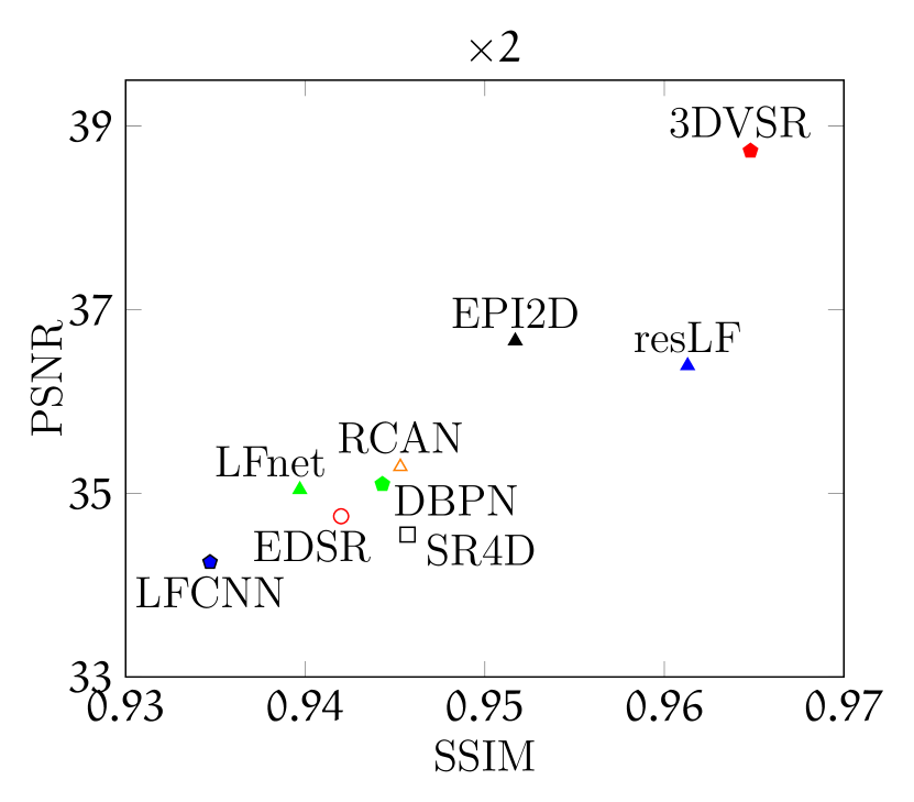
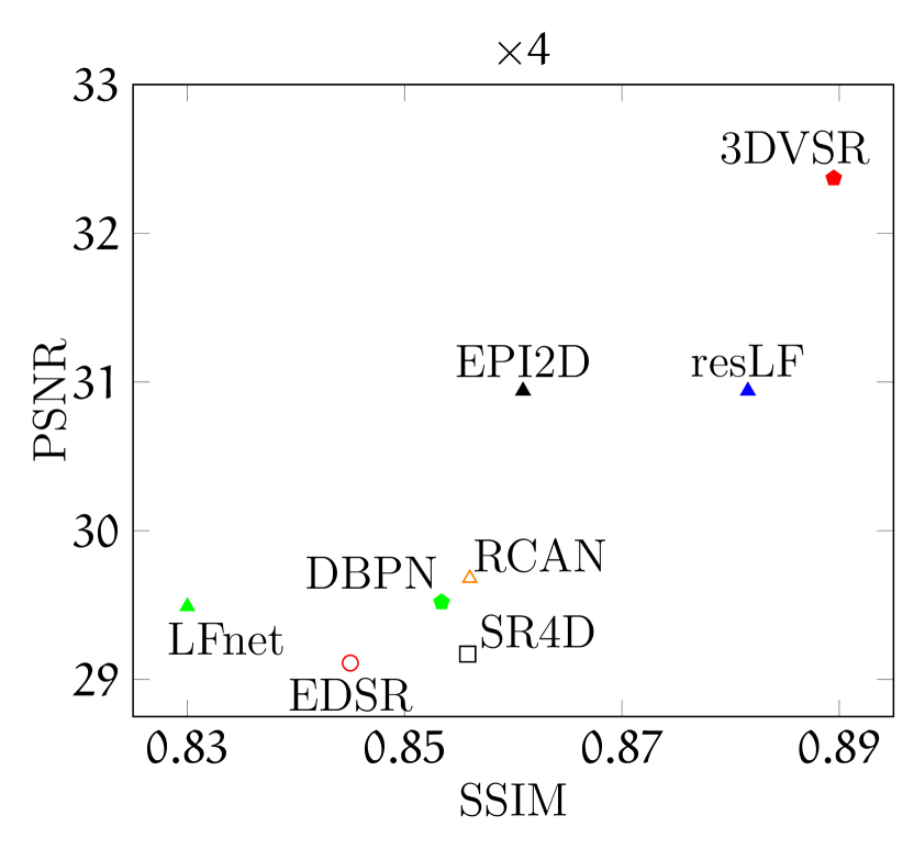
Figure 1: Spatial super-resolution results achieved by the proposed approach (3DVSR) and state-of-the-art SSR methods. The data points are averages of the performance metrics from 90 test scenes of 7 public datasets. ([8, 9, 10, 11, 12, 13, 14]). The proposed approach outperforms single image SR methods (EDSR [15], RCAN [16], DBPN [17]) and LF SSR methods (pcabm [18], LFCNN [19], LFnet [20], EPI2D [21], SR4D [22], resLF [23]).

An LF image can be characterized by a 4D array structure comprised of two spatial dimensions and two angular dimensions. In practice, it is considered as a 2D array of sub-aperture images (SAIs) that captures a scene from different perspectives. LF super-resolution distinguishes between spatial super-resolution (SSR), angular super-resolution (ASR), and angular-spatial super-resolution (ASSR). SSR aims for increasing the resolution of each SAI while ASR aims for generating new perspective images. ASSR, as its name indicates, involves both SSR and ASR and results in higher resolutions in all dimensions of an LF image. A straightforward approach for SSR is applying a single image super-resolution (SISR) technique in which each SAI is up-sampled independently. Thanks to comprehensive training dataset and mature development in the field of SISR, state-of-the-art approaches such as VDSR [24], EDSR [15], RCAN [16], RDN [25] can already reconstruct relatively good quality SAIs [7]. However, failing to incorporate angular information, this type of approach is easily surpassed by recent LF SSR methods (EPI2D [21], ResLF [23], SR4D [22]). Compared to SSR, there is less research attention to ASR and ASSR. Existing approaches such as VSYN [26], LFCNN [19], LFSR [27], Wang et al. [28], and Wu et al. [29, 30] employ convolutional neural network (CNN) for predicting novel SAI. However, their performances are still limited.

In this paper, a 3D EPI volume-based super-resolution approach (3DVSR) is proposed for dealing with LF super-resolution problems, i.e., ASR, SSR, and ASSR. As opposed to existing methods that rely on 2D slices of LF, i.e., epipolar images (EPIs) [21] or SAIs [23, 20], our approach makes use of a 3D projected version of LF, also known as 3D EPI volume [31]. The advantage of this volume structure is incorporating both spatial information in SAI and angular information in EPI. In addition, to fully exploit this 3D structure, we proposed a novel EPI volume refinement network (EVRN) built on 3D convolution operations and efficient deep learning techniques, i.e., global/local residual learning, dense connection, multi-path learning, and attention-based scaling. Experimental results show that EVRN substantially improves the reconstruction quality in all LF super-resolution problems. Fig. 1 presents the performance of the proposed approach compared to state-of-the-art methods for SSR. Peak signal to noise ratio (PSNR) and structural similarity index measure (SSIM) are employed as performance metrics. The proposed approach outperforms the existing approaches to a large extent in both SSR ${\mkern-2.0mu\times\mkern-2.0mu}2$ and ${\mkern-2.0mu\times\mkern-2.0mu}4$. Detail comparisons and evaluations are further discussed in Section 5.

The main contributions of this work are as follows. First, we proposed a novel 3D EPI volume-based framework for addressing various LF SR problems, i.e., ASR, SSR, and ASSR. Specifically, the framework comprises two consecutive stages, i.e., preliminary up-sampling stage and volume-based enhancement stage. The first stage allows different options to be used for up-sampling the input volume to the desired resolution. Then, in the second stage, the novel EVRN corrects the high-frequency information by incorporating both spatial information in SAI and angular information in 2D EPI to reconstruct a high-quality LF image. Such a two-stage model was first introduced by Fan et al. [32] for reconstructing a high-resolution SAI, but our approach is fundamentally different. In [32], outputs of the first stage are subjected to a view registration before feeding to a CNN to improve the quality of a targeted view. Although this method generates more references to support the enhancement of the targeted view, it destroys the EPI structure. Our approach, in contrast, preserves this structure in an EPI volume and introduces a novel EVRN to exploit this information for enhancing multiple views simultaneously. Compared to previous works which employed residual, dense, and attention techniques to reconstruct a high-resolution 2D image (RDN [25], RCAN [16]), the novelty of our EVRN lies in the introduction of attention-based multi-path learning, which targets spatial and angular aspects of the feature maps. As discussed in Section 5, this technique allows us to improve the performance of EVRN and, therefore, leads to a substantial enhancement of EPI volume output from the preliminary up-sampling stage. Secondly, a simple but effective Deep CNN model is proposed for preliminary up-sampling angular dimensions. Although its output quality is later greatly improved by EVRN, this model itself already surpasses existing approaches in ASR. Thirdly, an extensive evaluation is conducted on 90 challenging synthetic and real-world LF scenes from 7 public LF datasets. In this evaluation, we analyzed the performance of the proposed approach and compared it to state-of-the-art approaches.

The remainder of the paper is organized as follows. Section 2 briefly discusses related works categorized into optimization-based approaches and learning-based approaches. An overview of LF representation along with important notations is presented in Section 3. Section 4 and Section 5 respectively discuss the proposed approach and experimental results. Finally, we draw a conclusion in Section 6.

2 Related Work

In general, previous works can be categorized into two groups: optimization-based approaches and learning-based approaches.

2.1 Optimization-based approaches

In this type of approach, LF super-resolution is formulated as an optimization problem which typically consists of a data fidelity term directly composed from input LF image and a regularization term based on known priors. There are two main types of data terms that are used in the literature. One of them penalizes the coherence between low and high-resolution LF image pairs [33, 34, 35, 36]. The other enforces the Lambertian consistency across the directional dimension by warping SAIs from different view angles using pre-computed disparity maps  [37, 38, 36]. Compared to the data fidelity term, the choices of regularization terms are more diverse. Each work proposed to use a different prior in order to achieve a better output quality and with a feasible computation effort, i.e., total variation (TV) [37], bilateral TV[38], Markov Random Field (MRF) [34], Gaussian [33], Graph-based [39], sparsity [35].

In [34], Bishop et al. studied an explicit image formation model that characterizes the light field imaging process by spatially-variant point spread functions (PSFs). The PSFs were derived under Gaussian optics assumptions and employed in a Bayesian framework for super-resolution. In [33], Mitra et al. showed that 4-D patches of different disparities have different intrinsic dimensions and proposed to learn a Gaussian prior for each quantized disparity value. These priors were then employed to inference high-resolution 4-D patches under the Maximum a posterior (MAP) criterion. LF super-resolution was modeled as a continuous optimization problem using a variational framework in [37]. Disparity maps were extracted by local estimation of pixel-wise slope in EPI. The data fidelity term was constructed by warping surrounding views with the estimated disparity maps and masking with occlusion maps, while total variation was used for regularization. In [38], Tran et al. treated LF super-resolution as a multi-frame super-resolution problem in which degradation process is modeled by three operators: down-sampling, blurring, and warping. A variational optimization approach was employed to estimate disparity maps used by the warping operator and bilateral TV was employed as an image prior. In [35], Alain et al. proposed a patch-based super-resolution approach making use of a 5D transform filter that consists of 2D DCT transform, 2D shape-adaptive DCT and 1D haar wavelet. By a proper selection of 5D patches, a transformed signal exposes a high degree of sparsity which can be employed as a prior to regularise a $L^{2}$ data term. In [39], Rossi et al. proposed an approach which couples two data-terms with a graph-based regularizer. A graph-based prior regularizes high-resolution SAIs by enforcing the geometric light field structure. Block matching was employed in their work for the estimation of disparity values and the construction of the graph map.

2.2 Learning-based approaches

(a)

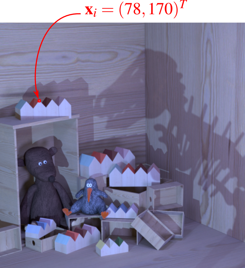
(b)

(c)

Figure 2: 4D Light field representation. (a) Two-plane parameterisation. (b) A sub-aperture image of scene dino [9] at angular location $\boldsymbol{\theta}_{i}=(6,3)^{T}$. (c) An angular patch image at spatial location $\mathfrak{\textbf{x}}_{i}=(78,170)^{T}$.

The earliest work which applies deep learning for reconstructing high-resolution LF is [40]. The authors employed the SISR approach from [41] for SSR and proposed a CNN-based solution for ASR in which novel views depending on its position will be synthesized from a vertical pair, a horizontal pair, or four neighbors. An improved version was described in [19] where SISR was applied to each SAI separately, and learning variables were shared in the ASR network. In [26], Kalantari et al. proposed to generate novel SAIs by exploiting disparity information in a two-stage CNN. The first stage predicts disparity maps from a pre-computed cost-volume, and the second stage synthesizes novel views from input images that are warped using predicted disparity maps. In [18], a patch-based approach that employs linear subspace projection was presented. A linear mapping function between low and high subspaces of low and high LF patch volume was learned from a training dataset and applied to new LF images. The authors used block matching to find matched 2D patches and extract aligned patch volumes. Principal component analysis (PCA) was then employed to reduce patch volumes’ dimensions and project them into subspaces. The mapping function was computed in the form of a $l_{2}$-norm regularized least square problem. Fan et al. [32] proposed a two-stage approach for SSR. In the first stage, each SAI was upscaled using the SISR method from VDSR [24]. The output was then registered to a reference SAI by locally searching similar patches. Both reference image and registered images were fed into a CNN network in the second stage to reconstruct high-resolution SAI at the reference position. Similarly, Yuan et al. [21] proposed another two-stage approach. In the first stage, EDSR [15] was employed to super-resolute SAIs. In the second stage, the output of SISR was then enhanced by a refinement CNN which relies on 2D EPI. In [27], Gul et al. proposed an approach targeting lenslet images captured by plenoptic cameras [4, 5]. Microlens image patches were used as input to two separate networks, i.e., one for ASR and the other for SSR. However, the fully connected layers employed in these networks limited its application to a certain angular resolution. Wang et al. [20] developed a bidirectional recurrent CNN approach for spatially up-sampling 4D LF images. They employed multi-scale fusion layers for future extraction to accumulate contextual information. Two networks for vertical and horizontal image stacks were learned separately, and a stack generalization technique was employed to obtain a complete set of images. In [28], the authors proposed a two-step approach to synthesize novel views. In the first step, a learnable interpolation approach is employed to generate intermediate volumes, which are then refined in the second step through a 3D CNN. However, since the architecture of the 3D CNN is simple, the performance of this refinement step is limited. In [29] and  [30] Wu et al. proposed two novel approaches for LF view synthesis based on EPI structure. In [29], a set of shared EPIs is created for a discrete set of shear values which is then up-sampled and scored by an evaluation CNN to create a cost volume. The 2D slices output from fusing the cost volume are then subjected for a high-resolution EPI calculation based on a pyramid decomposition-reconstruction technique. In [30], the authors model the view synthesis as a learning-based detail restoration on 2D EPIs. They proposed a three-step framework, namely “blur-restoration-deblur” that employs the blurring operator for blur step, a CNN for restoration step, and a non-bind deblur operation for the last step. To fully exploit the 4D structure of LF images, Yeung et al. [22] proposed to apply 4D convolution for SSR. The 4D convolution function was implemented as spatial-angular separable convolution, which allows extracting feature maps from both spatial and angular domains. In [23], Zhang et al. proposed a residual CNN-based approach for reconstructing LF images with higher spatial resolution. The network takes in image stacks from four different angles and predicts a high-resolution image at the center position. According to the difference in angular position, it requires six different networks for a complete reconstruction of the 4D LF image.

Figure 3: 2D EPI projection of 4D LF scene horses [8]. top-left SAI at $\boldsymbol{\theta}_{i}=[\rho_{i},\tau_{i}]^{T}$; top-right vertical EPI ($\Sigma_{x_{i},\rho_{i}}$); bottom horizontal EPI ($\Sigma_{y_{i},\tau_{i}}$).

3 Light field Notation

Light field refers to the concept of acquiring a complete description of light rays emitted from a scene and traverse in space. It can be well parameterized by the 7D plenoptic function $\boldsymbol{L}\big{(}p_{x},p_{y},p_{z},\theta,\phi,\lambda,t\big{)}$ [4] which returns the radiance (intensity) of a line beam observed at a point $\big{(}p_{x},p_{y},p_{z}\big{)}$ in space, along a grazing direction $\big{(}\theta,\phi\big{)}$, at a time $t$ and wavelength $\lambda$. In practice, it is of interest to capture only a snapshot of the function (at a fixed time) and simplify the spectral information by using only 3 color components (i.e. red, green, blue). By removing the time and wavelength parameters, we are left with a 5-parameters function, also known as 5D plenoptic function [42], which allows us to describe the intensity of any light ray in 3D space regardless the viewpoint position and the change of light direction. One more parameter can be omitted from the function, if one assumes that the direction of a light ray is unchanged and considers only the light intensity being visible at a specific position, i.e. placing of cameras. This is also the common setup of light field imaging which results in a 4D light field [42] or Lumigraph [43]. Under the two plane parameterization, each ray is indexed with a 4D coordinate by its intersection with two parallel planes, as depicted in Figure 2a.

$$\boldsymbol{L}\colon\Omega{\mkern-2.0mu\times\mkern-2.0mu}\Pi\rightarrow\mathbb{R},\qquad(\mathfrak{\textbf{x}},\boldsymbol{\theta})\rightarrow\boldsymbol{L}(\mathfrak{\textbf{x}},\boldsymbol{\theta})$$ (1)

where $\mathfrak{\textbf{x}}=[x,y]^{T}$ and $\boldsymbol{\theta}=[\rho,\tau]^{T}$ denote coordinate pairs in the spatial plane $\Omega\subset\mathbb{R}^{2}$ and in the directional plane $\Pi\subset\mathbb{R}^{2}$ respectively. In practice, the value of this function can be a vector of 3 color components (i.e., RGB color light field) and the two planes are discretized by the sampling rate of capturing devices (e.g., sensor size, number of cameras,…).

For a better observation and analysis, various ways to visualize 4D LF are introduced in the literature. Common visualizations are using 2D slices, i.e., sub-aperture image (SAI), angular patch image (API), or epipolar image (EPI). By fixing the directional index $\boldsymbol{\theta}=\boldsymbol{\theta}_{i}$ or the spatial index $\mathfrak{\textbf{x}}=\mathfrak{\textbf{x}}_{i}$, one can respectively obtain a SAI $\boldsymbol{L}(\mathfrak{\textbf{x}},\boldsymbol{\theta}_{i})$ or an API $\boldsymbol{L}(\mathfrak{\textbf{x}}_{i},\boldsymbol{\theta})$. Fig. 2 (b),(c) are examples of a sub-aperture image and an angular patch extracted from a 4D synthetic light field image, dino [9]. The resolution of this light field is 512${\mkern-2.0mu\times\mkern-2.0mu}$512${\mkern-2.0mu\times\mkern-2.0mu}$9${\mkern-2.0mu\times\mkern-2.0mu}$9, where 512${\mkern-2.0mu\times\mkern-2.0mu}$512 is the spatial resolution and 9${\mkern-2.0mu\times\mkern-2.0mu}$9 is the angular resolution. The angular patch consists of pixels, each at the same spatial location $\mathfrak{\textbf{x}}_{i}=(78,170)^{T}$ on a sub-aperture. An EPI can be acquired by fixing one index in the spatial plane and one index in the angular plane while varying the remaining two indices. By fixing vertical indices, i.e., $y\!=\!y_{i},\tau\!=\!\tau_{i}$, we have the horizontal EPI $\Sigma_{y_{i},\tau_{i}}(x,\rho)=\boldsymbol{L}\big{(}[x,y_{i}]^{T},[\rho,\tau_{i})]^{T}\big{)}$. A similar procedure applies to vertical EPI $\Sigma_{x_{i},\rho_{i}}(y,\tau)$. Fig. 3 illustrates the two types of EPIs.

As pointed out in [37], a point in 3D space is projected onto a line in EPI whose slope is decided by the depth of this point. For example, in Figure 3 the point located at $(x_{i},y_{i})$ projected onto two lines in horizontal EPI ($\Sigma_{y_{i},\tau_{i}}$) and vertical EPI ($\Sigma_{x_{i},\rho_{i}}$). Notice that all letters crossed by the line $y=y_{i}$ (i.e., dotted green line) reside on the same depth and result in identical slope in horizontal EPI $\Sigma_{y_{i},\tau_{i}}$. This property of EPI represents the geometric information of the scene and was exploited in many LF image processing applications (i.e. disparity estimation [31, 37], super-resolution [37, 21]). In this work, we consider a 3D version of EPI, namely EPI volume [31], in which the second spatial dimension is added. The intuition behind this volume data is the combination of both spatial coherence (i.e. $x$ vs. $y$) and EPI coherence (i.e. $x$ vs. $\rho$) that can be employed for reconstructing high-quality LF image. Horizontal EPI volume $\boldsymbol{V}_{\tau_{i}}$ and vertical EPI volume $\boldsymbol{V}_{\rho_{i}}$ are defined in Equation 2. An EPI volume is an orthogonal 3D slide through 4D LF and can be considered as a stack of 2D EPI along a spatial axis, e.g., $\boldsymbol{V}_{\tau_{i}}$ is constructed by stacking horizontal EPI $\Sigma_{y_{i},\tau_{i}}$ along spatially vertical axis $y$.

$$\begin{split}\boldsymbol{V}_{\tau_{i}}\colon\mathbb{R}^{3}\rightarrow\mathbb{R},\qquad(x,\rho,y)\rightarrow\boldsymbol{L}\left(\begin{bmatrix}x\\ y\end{bmatrix},\begin{bmatrix}\rho\\ \tau_{i}\end{bmatrix}\right)\\ \boldsymbol{V}_{\rho_{i}}\colon\mathbb{R}^{3}\rightarrow\mathbb{R},\qquad(y,\tau,x)\rightarrow\boldsymbol{L}\left(\begin{bmatrix}x\\ y\end{bmatrix},\begin{bmatrix}\rho_{i}\\ \tau\end{bmatrix}\right)\end{split}$$ (2)

Figure 4: Overview of 3D EPI volume SR framework. The framework consists of a preliminary up-sampling stage and an enhancement stage. The earlier stage includes a preliminary spatial SR block (PSSR) and a preliminary angular SR block (PASR). The later stage includes an EPI volume refinement network (EVRN).

This work assumes that 4D LF image has the resolution of $W{\mkern-2.0mu\times\mkern-2.0mu}H{\mkern-2.0mu\times\mkern-2.0mu}A{\mkern-2.0mu\times\mkern-2.0mu}A$, where $H,W\in\mathbb{N}^{+}$ respectively represent the height and width of each SAI and $A\!=\!2K+1,K\!\in\!\mathbb{N}^{+}$ denotes the angular resolution. The resolutions of $\rho$-axis and $\tau$-axis are set equally, since this square array of views is commonly used in literature [18, 19, 20, 21, 22, 23] and available in public dataset [8, 9, 10, 11, 12, 13, 14]. The resolution of horizontal EPI volume $\boldsymbol{V}_{\tau_{i}}$ and vertical EPI volume $\boldsymbol{V}_{\rho_{i}}$ are then $W{\mkern-2.0mu\times\mkern-2.0mu}A{\mkern-2.0mu\times\mkern-2.0mu}H$ and $H{\mkern-2.0mu\times\mkern-2.0mu}A{\mkern-2.0mu\times\mkern-2.0mu}W$ respectively.

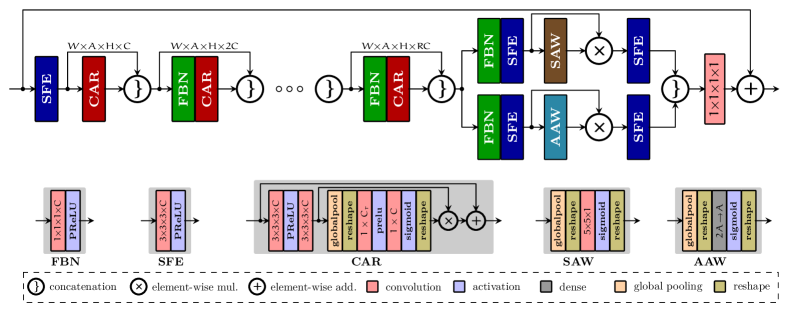
Figure 5: The network architecture of the proposed EPI volume refinement network (EVRN)

4 Methodology

4.1 Overview of the Proposed Approach

The proposed approach targets the super-resolution of 3D projected versions of a 4D LF image. Instead of directly up-sampling a 4D LF image (e.g, SR4D [22]), we first decompose it into a complete set of 3D EPI volumes. Each EPI volume is then super-resolved to its desired resolution. The high-resolution sets of EPI volumes are finally merged to form the final high-resolution 4D output. Fig. 4 illustrates the overall process of the proposed EPI volume SR framework. The framework is comprised of two main processing stages: a preliminary up-sampling stage and a volume enhancement stage. The first stage involves two tasks: preliminary spatial super-resolution (PSSR) and preliminary angular super-resolution (PASR). The second stage includes an EPI volume-based refinement network (EVRN). Given a 3D EPI volume ($\boldsymbol{V}_{l}$) with the resolution of $W{\mkern-2.0mu\times\mkern-2.0mu}A{\mkern-2.0mu\times\mkern-2.0mu}H$, PSSR and PASR sequentially up-sample the spatial resolution to $\contour[1]{black}{$\zeta$}_{\mathfrak{\textbf{x}}}W{\mkern-2.0mu\times\mkern-2.0mu}\contour[1]{black}{$\zeta$}_{\mathfrak{\textbf{x}}}H$ and the angular resolution to $\contour[1]{black}{$\zeta$}_{\boldsymbol{\theta}}A$, where $\contour[1]{black}{$\zeta$}_{\mathfrak{\textbf{x}}}$ and $\contour[1]{black}{$\zeta$}_{\boldsymbol{\theta}}$ are spatial and angular scaling factor respectively. This preliminarily up-sampling volume is provided as an input to EVRN which will, in turn, refine the 3D EPI structure and return an enhanced high-resolution volume. PSSR and PASR can be applied separately or jointly depending on SR applications (i.e., SSR, ASR, and ASSR).

1

2Function VSR($\boldsymbol{L}_{l}$, $\varepsilon$, $\mathcal{F}$):

       $\{\boldsymbol{V}\}_{\varepsilon}:=\texttt{Slice}(\boldsymbol{L}_{l},\varepsilon)$

        $\triangleright$ Extract $\varepsilon$-axis volumes

       $\{\boldsymbol{V}\}_{*}:=\{\}$

        $\triangleright$ Initialize empty volume set

3       for $\boldsymbol{V}$ in $\{\boldsymbol{V}\}_{\varepsilon}$ do

4             $\{\boldsymbol{V}\}_{*}:=\{\boldsymbol{V}\}_{*}+\mathcal{F}(\boldsymbol{V})$

5       end for

      $\boldsymbol{L}_{h}:=\texttt{Merge}(\{\boldsymbol{V}\}_{*},\varepsilon)$

        $\triangleright$ Reconstruct 4D LF

6       return $\boldsymbol{L}_{h}$

7      

8 end

Algorithm 1 Volume-based super-resolution (VSR) function

Input: $\boldsymbol{L}_{l}$

Output: $\boldsymbol{L}_{h}$

1 $\boldsymbol{L}:=\boldsymbol{L}_{l}$

2 if spatial super-resolution then

       $\mathcal{F}:=\mathcal{R}\big{(}\mathcal{S}(\cdot)\big{)}$

        $\triangleright$ Apply PSSR and EVRN

3       $\boldsymbol{L}:=0.5\Big{(}\texttt{VSR}(\boldsymbol{L},\tau,\mathcal{F})+\texttt{VSR}(\boldsymbol{L},\rho,\mathcal{F})\Big{)}$

4      

5 else if angular super-resolution then

6       if spatial super-resolution then

             $\mathcal{F}:=\mathcal{S}(\cdot)$

              $\triangleright$ Apply only PSSR

7             $\boldsymbol{L}:=\texttt{VSR}(\boldsymbol{L},\tau,\mathcal{F})$

8       end if

      $\mathcal{F}:=\mathcal{R}\big{(}\mathcal{A}(\cdot)\big{)}$

        $\triangleright$ Apply PASR and EVRN

       $\boldsymbol{L}:=\texttt{VSR}(\boldsymbol{L},\tau,\mathcal{F})$

        $\triangleright$ Upscale $\rho$-axis

       $\boldsymbol{L}:=\texttt{VSR}(\boldsymbol{L},\rho,\mathcal{F})$

        $\triangleright$ Upscale $\tau$-axis

9      

10 end if

11$\boldsymbol{L}_{h}:=\boldsymbol{L}$

Algorithm 2 Spatial-angular super-resolution of 4D LF

The function VSR in Algorithm 1 describes the application of the proposed framework for the reconstruction of high resolution LF image. VSR takes in three paramters: a low-resolution LF ($\boldsymbol{L}_{l}$), a directional axis ($\varepsilon\!\in\!\{\rho,\tau\}$), and a volume-based SR function ($\mathcal{F}$). The directional axis is needed to determine the direction of 3D projection which will results in either vertical volume ($\varepsilon\!=\!\rho$) or horizonal volume ($\varepsilon\!=\!\tau$). The volume-based SR function encodes the configuration of PSSR and PASR as in Fig. 4, i.e., only PSSR, only PASR, and both. The procedure of VSR is as follow. First, a set of EPI volumes are extracted from the input $\boldsymbol{L}_{l}$ (line $2$). Depending on $\varepsilon$, function $\texttt{Slice}(\cdot)$ will return either horizontal volume or vertical volume set $\big{(}\{\boldsymbol{V}\}_{\varepsilon}=\{\boldsymbol{V}_{\varepsilon_{i}},i=1,..,A\}\big{)}$. Next, a high resolution volume set $\{\boldsymbol{V}\}_{*}$ is acquired by applying volume SR function ($\mathcal{F}$) to each volume in $\{Vol\}_{\varepsilon}$ (line $3-6$). Finally, we combine 3D volumes in $\{Vol\}_{*}$ to form a high-resolution 4D output (line $7$).

The applications of VSR function in SSR, ASR, and ASSR are described in Algorithm 2. In the case of SSR, $\mathcal{F}$ is comprised of PSSR, denoted as $\mathcal{S}$, and EVRN denoted as $\mathcal{R}$, (line 3). VSR is applied to horizontal and vertical volumes separately and then the output LFs are averaged (line 4). In the case of ASR, $\mathcal{F}$ is set as PASR, denoted as $\mathcal{A}$, followed by EVRN (line 10). The super-resolution of horizontal volumes (line 11) and vertical volumes (line 12) will increase the angular resolution to $\contour[1]{black}{$\zeta$}_{\boldsymbol{\theta}}A\times A$ and $\contour[1]{black}{$\zeta$}_{\boldsymbol{\theta}}A\times\contour[1]{black}{$\zeta$}_{\boldsymbol{\theta}}A$ respectively. As for ASSR, a similar procedure to ASR is applied, except that PSSR is previously employed to spatially up-sample the input light field (line 7,8).

4.2 EPI Volume Refinement Network

The proposed network bases on global residual learning architecture that is implemented with a long skip connection and an element-wise addition as illustrated in Fig. 5. Global residual learning allows EVRN to avoid learning complicated transformation and focus on the reconstruction of high-frequency information differing between low and high-resolution EPI volume. 3D convolutional kernels are utilized in our network instead of 2D convolutions since this type of kernel was shown to be effective with 3D EPI volume data [31]. EVRN is comprised of two parts: attention-based residual learning extracts densely residual-based features and attention-based multi-path learning reconstructs high-frequency information.

4.2.1 Attention-based Residual Learning

This part consists of a shallow feature extraction layer (SFE) followed by $R$ local residual learning blocks. Dense connection [44] is employed to alleviate gradient vanishing and improve signal propagation. With this setup, the feature maps of all preceding layers are combined and used as an input to the current layer. Since the accumulated feature size gets bigger after each layer and demands a high computational effort, we decide to compress the concatenated features by a feature bottle-neck layer (FBN). FBN consisting of a $1{\mkern-2.0mu\times\mkern-2.0mu}1{\mkern-2.0mu\times\mkern-2.0mu}1{\mkern-2.0mu\times\mkern-2.0mu}C$ convolutional layer followed by a PReLU activation layer will reduce the dense-feature size to $C$ channels before inputting to a channel attention-based residual layer (CAR) as in Fig. 5.

For the local residual learning block, we follow RCAN [16] to integrate channel attention [45] for adaptively scaling residual features. As shown in  [16], this technique improves the reconstruction quality of high-resolution images. The architecture of CAR is comprised of a well-known feature extraction combination conv-prelu-conv followed by a channel attention weighting block (CAW). CAW starts with a global average pooling layer which collapses an input feature from $W{\mkern-2.0mu\times\mkern-2.0mu}A{\mkern-2.0mu\times\mkern-2.0mu}H{\mkern-2.0mu\times\mkern-2.0mu}C$ to $1{\mkern-2.0mu\times\mkern-2.0mu}1{\mkern-2.0mu\times\mkern-2.0mu}1{\mkern-2.0mu\times\mkern-2.0mu}C$. It is then reshaped to $1{\mkern-2.0mu\times\mkern-2.0mu}C$ and is followed by a 1D down-sampling convolution ($1{\mkern-2.0mu\times\mkern-2.0mu}C_{r}$) and 1D up-sampling convolution ($1{\mkern-2.0mu\times\mkern-2.0mu}C$). Here $C_{r}=\frac{C}{r}$ with $r$ is a predefined reduction ratio. After going through a sigmoid activation layer, the $1{\mkern-2.0mu\times\mkern-2.0mu}C$ scaling weight is reshaped and broadcasted to the form $W{\mkern-2.0mu\times\mkern-2.0mu}A{\mkern-2.0mu\times\mkern-2.0mu}H{\mkern-2.0mu\times\mkern-2.0mu}C$ being ready for an element-wise multiplication with the input feature.

4.2.2 Attention-based Multi-Path Learning

This part is comprised of two separate learning paths targeting spatial and angular aspects of the feature maps. Each path includes an FBN, two SFEs, and an attention-based weighting block as in Fig. 5. There are two types of attention-based weighting, one is for spatial feature dimensions denoted as SAW and the other is for angular feature dimension denoted as AAW. FBN is employed to reduce the size of densely connected feature-maps generated by the residual learning part. After this block, the feature size is reduced from $(R+1)C$ channels to $C$ channels. The reduced feature map is fed to an SFE whose output is refined by an element-wise multiplication with attention weights computed by AAW or SAW. After the second SFE, the feature maps from the two paths are concatenated and squeezed to form the final residual feature map. The high-resolution EPI volume is acquired by adding up the residual information to the preliminarily up-sampled volume.

SAW consists of a global pooling, a 2D convolution, and a sigmoid activation layer. In global pooling layer, Average Pooling ($P_{avg}$) and Max Pooling ($P_{max}$) are applied to the input feature $F\in\mathbb{R}^{W{\mkern-2.0mu\times\mkern-2.0mu}A{\mkern-2.0mu\times\mkern-2.0mu}H{\mkern-2.0mu\times\mkern-2.0mu}C}$ and results in $F_{avg},\ F_{max}\in\mathbb{R}^{W{\mkern-2.0mu\times\mkern-2.0mu}1{\mkern-2.0mu\times\mkern-2.0mu}H{\mkern-2.0mu\times\mkern-2.0mu}1}$. These feature maps are then concatenated and reshaped to form the global pooling feature $F_{pool}\in\mathbb{R}^{W{\mkern-2.0mu\times\mkern-2.0mu}H{\mkern-2.0mu\times\mkern-2.0mu}2}$. We then applied a 2D convolution with kernel size $5{\mkern-2.0mu\times\mkern-2.0mu}5{\mkern-2.0mu\times\mkern-2.0mu}1$ followed by a sigmoid activation function. These weighting values are then reshaped and broadcasted to the form $W{\mkern-2.0mu\times\mkern-2.0mu}A{\mkern-2.0mu\times\mkern-2.0mu}H{\mkern-2.0mu\times\mkern-2.0mu}C$ for an element-wise multiplication. The following equation summarizes the computation of spatial attention weights.

$$W_{s}(F)=\sigma\bigg{(}f_{5{\mkern-2.0mu\times\mkern-2.0mu}5{\mkern-2.0mu\times\mkern-2.0mu}1}\Big{(}\big{[}P_{avg}(F);P_{max}(F)\big{]}\Big{)}\bigg{)}$$ (3)

AAW consists of a global pooling, a fully-connected, and a sigmoid activation layer. Given an input feature $F\in\mathbb{R}^{W{\mkern-2.0mu\times\mkern-2.0mu}H{\mkern-2.0mu\times\mkern-2.0mu}A{\mkern-2.0mu\times\mkern-2.0mu}C}$, we follow a similar procedure as of SAW to compute global pooling features $F_{pool}\in\mathbb{R}^{2A}$. Here, $P_{avg}$ and $P_{max}$ are applied to spatial and channel dimensions of the input feature map and the output features are concatenated along the angular dimension. We then compute $A$ weighting values by applying a fully connected layer followed by a sigmoid activation function. Equation 4 outlines this computation.

$$W_{a}(F)=\sigma\bigg{(}D_{2A:A}\Big{(}\big{[}P_{avg}(F);P_{max}(F)\big{]}\Big{)}\bigg{)}$$ (4)

4.3 Preliminary spatial super-resolution

Given an EPI volume $\boldsymbol{V}_{l}$ with a resolution of $W{\mkern-2.0mu\times\mkern-2.0mu}A{\mkern-2.0mu\times\mkern-2.0mu}H$ as an input, the output of PSSR is an EPI volume $\boldsymbol{V}_{h}$ with a resolution of $\contour[1]{black}{$\zeta$}_{\mathfrak{\textbf{x}}}W{\mkern-2.0mu\times\mkern-2.0mu}A{\mkern-2.0mu\times\mkern-2.0mu}\contour[1]{black}{$\zeta$}_{\mathfrak{\textbf{x}}}H$, where $\contour[1]{black}{$\zeta$}_{\mathfrak{\textbf{x}}}$ is a spatial scaling factor (i.e., $2,4$). The procedure of PSSR is as follows. First, 2D images (SAIs) along angular dimension ($\boldsymbol{V}_{l}(x,i,y),i\!=\!1,2,..,A$) are extracted from the input volume. Secondly, each image is separately super-resolved to the desired resolution by a SISR method. Finally, we combine these up-sampled images to form the output volume $\boldsymbol{V}_{h}$, see Fig. 4.

In this work, deep learning-based methods (i.e., EDSR [15], RCAN [16]) are employed to up-sample SAIs. With many advanced learning architectures introduced lately and sufficient training data, deep learning-based approaches easily outperform optimization-based approaches and provide state-of-the-art performance in the SISR task. However, as pointed out in the literature [21, 20, 22, 23] that SISR alone did not perform well on light field images due to missing the contribution of external information shared across multiple SAIs. This such information is well contained in an EPI volume and is exploited in the proposed EVRN to enhance the output of SISR. As will be shown later in the experimental result, the proposed approach substantially improves the reconstruction quality of SISR on both challenging synthetic and real-world LF data.

4.4 Preliminary angular super-resolution

In this stage, a novel perspective image is generated for each consecutive pair of SAIs in the input volume. This task is done by a novel view synthesis module (NVS) as depicted in Figure 4. Given an EPI volume $\boldsymbol{V}_{l}$ with a resolution of $W{\mkern-2.0mu\times\mkern-2.0mu}A{\mkern-2.0mu\times\mkern-2.0mu}H$ as an input, the output of PASR is an EPI volume $\boldsymbol{V}_{h}$ with a resolution of $W{\mkern-2.0mu\times\mkern-2.0mu}(2A\!-\!1){\mkern-2.0mu\times\mkern-2.0mu}H$. The angular resolution of the volume is up-sampled by a scaling factor of $\contour[1]{black}{$\zeta$}_{\boldsymbol{\theta}}=\frac{2A\!-\!1}{A}$.

The synthesis of a novel view can be seen as the interpolation of a novel pixel along a line on an EPI image, see Fig. 3. This task is indeed trivial if the slope of this line, also referred to as disparity value [37], is known in advance. Therefore, many previous approaches [37, 26, 38] proposed to firstly estimate disparity maps and then exploit them for synthesizing novel views. However, as shown in [19, 27], this explicit estimation of a disparity map is not necessary since a learning-based approach which directly inferences novel views can already provide better performance. In this work, two different approaches of NVS are evaluated, i.e., nvs-cnn and nvs-mean. nvs-cnn is the proposed end-to-end CNN learning to synthesize a novel view from an input image pair. In nvs-mean, the new view is computed by simply averaging the two input images. As will be shown in Section 5.4, this straightforward approach can provide good results in the case of narrow baseline LF images captured by plenoptic cameras [4, 5].

Figure 6: The network architecture of the proposed CNN-based method for PASR

The network architecture of nvs-cnn is presented in Fig. 6. Similar to EVRN, global/local residual learning and dense connection are employed in the proposed network. We stack two input images to form an input feature $X\in\mathbb{R}^{W{\mkern-2.0mu\times\mkern-2.0mu}H{\mkern-2.0mu\times\mkern-2.0mu}2}$. A shallow feature extraction layer consisting of a 2D convolutional kernel $3{\mkern-2.0mu\times\mkern-2.0mu}3{\mkern-2.0mu\times\mkern-2.0mu}C^{\prime}$ followed by a PReLU activation is applied to $X$. This results in a feature map $F_{0}\in\mathbb{R}^{W{\mkern-2.0mu\times\mkern-2.0mu}H{\mkern-2.0mu\times\mkern-2.0mu}C^{\prime}}$. After going through $R^{\prime}$ layers of residual blocks, we get a residual feature map $F_{R^{\prime}}\in\mathbb{R}^{W{\mkern-2.0mu\times\mkern-2.0mu}H{\mkern-2.0mu\times\mkern-2.0mu}C^{\prime}}$ which is added to $F_{0}$ and then squeezed by a 2D convolution kernel $3{\mkern-2.0mu\times\mkern-2.0mu}3{\mkern-2.0mu\times\mkern-2.0mu}1$ to acquire a novel perspective image ($I\in\mathbb{R}^{W{\mkern-2.0mu\times\mkern-2.0mu}H}$). For residual block, we use a simple design that consists of a bottleneck layer, i.e., 2D convolution kernel ($1{\mkern-2.0mu\times\mkern-2.0mu}1{\mkern-2.0mu\times\mkern-2.0mu}C^{\prime}$) followed by a PReLU, and a common combination conv-prelu-conv as in Fig. 6.

5 Experimental Results

5.1 Dataset and training

Table 1: Summary of training and test dataset

Datasets	Type	Angular	Training	Test
HCI13[8]	synthetic	$9{\mkern-2.0mu\times\mkern-2.0mu}9$	$5$	$2$
HCI17[9]	synthetic	$9{\mkern-2.0mu\times\mkern-2.0mu}9$	$20$	$4$
InSyn[10]	synthetic	$9{\mkern-2.0mu\times\mkern-2.0mu}9$	$31$	$8$
StGantry[11]	real-world	$17{\mkern-2.0mu\times\mkern-2.0mu}17$	$9$	$3$
StLytro[12]	real-world	$14{\mkern-2.0mu\times\mkern-2.0mu}14$	$250$	$53$
InLytro[13]	real-world	$15{\mkern-2.0mu\times\mkern-2.0mu}15$	$28$	$8$
EPFL[14]	real-world	$15{\mkern-2.0mu\times\mkern-2.0mu}15$	$81$	$12$
Sum	-	-	$424$	$90$

Seven published light field datasets, listed in Table 1, are employed for training and testing the proposed approach. There are three synthetic datasets generated by 3D object models and blender software [8, 9, 10]. The other four datasets are real-world data captured by Illum cameras [12, 13, 14] and a gantry setup [11]. While the synthetic scenes have the same angular resolution of $9{\mkern-2.0mu\times\mkern-2.0mu}9$, the angular resolution of real-world scenes varies from $14{\mkern-2.0mu\times\mkern-2.0mu}14$ to $17{\mkern-2.0mu\times\mkern-2.0mu}17$. To have an uniform light field data for training and testing, we follow the previous work [20, 21, 22, 23] to remove the border views and keep only $9{\mkern-2.0mu\times\mkern-2.0mu}9$ sub-aperture images in the middle.

5.1.1 Training EVRN

The LF images in the training set are transformed into YCbCr color space and only Y channel data is used for training. In inference phase, we apply the trained network to each color space separately and then convert them back to RGB color image. Each LF image is spatially cropped into 4D patch ($P_{H}\in\mathbb{R}^{48{\mkern-2.0mu\times\mkern-2.0mu}48{\mkern-2.0mu\times\mkern-2.0mu}9{\mkern-2.0mu\times\mkern-2.0mu}9}$) with a stride of 16 pixels. Plain patches which do not include texture information are ignored. For each 2D patch with the size of $48{\mkern-2.0mu\times\mkern-2.0mu}48$ from $P_{H}$, we apply bicubic down-sampling with a scaling factor $\contour[1]{black}{$\zeta$}_{\mathfrak{\textbf{x}}}$ ($\contour[1]{black}{$\zeta$}_{\mathfrak{\textbf{x}}}=2,4$) to acquire a low spatial resolution patch $P_{LS}\in\mathbb{R}^{\contour[1]{black}{$\zeta$}^{-1}_{\mathfrak{\textbf{x}}}48{\mkern-2.0mu\times\mkern-2.0mu}\contour[1]{black}{$\zeta$}^{-1}_{\mathfrak{\textbf{x}}}48{\mkern-2.0mu\times\mkern-2.0mu}9{\mkern-2.0mu\times\mkern-2.0mu}9}$. Each 2D patch in $P_{LS}$ is then up-sampled using SISR method to generate a spatial pre-scaling 4D patch $P_{S}$. A low angular resolution 4D patch ($P_{LA}\in\mathbb{R}^{48{\mkern-2.0mu\times\mkern-2.0mu}48{\mkern-2.0mu\times\mkern-2.0mu}5{\mkern-2.0mu\times\mkern-2.0mu}5}$) is extracted from $P_{H}$ by removing 2D patches at angular position $(\rho_{i},\tau_{i})$, where $(\rho_{i}\bmod 2)\lor(\tau_{i}\bmod 2)=1$. We then up-sampled $P_{LA}$ using the technique discussed in Section 4.4 to acquire angular pre-scaling 4D patch $P_{A}$. An angular-spatial pre-scaling 4D patch $P_{SA}$ is generated by applying the same procedure to $P_{S}$. At this point, we have three 4D patch pairs $\big{(}\{P_{S}\},\{P_{H}\}\big{)}$, $\big{(}\{P_{A}\},\{P_{H}\}\big{)}$, and $\big{(}\{P_{SA}\},\{P_{H}\}\big{)}$ to train EVRN for SSR, ASR, and ASSR respectively. For each 4D patch pair, e.g., $\big{(}\{P_{S}\},\{P_{H}\}\big{)}$, a 3D EPI volume pair $\big{(}\{V_{L}\},\{V_{H}\}\big{)}$ is formed by extracting and combining the horizontal and vertical EPI volumes from each 4D patch set.

Table 2: Performance analysis of various model configurations.

Models	Synthetic		Real-world
	PSNR	SSIM	PSNR	SSIM
model 1	38.61	0.9613	38.09	0.9581
model 2	38.63	0.9613	38.13	0.9588
model 3	38.77	0.9627	38.21	0.9592

Table 3: Ablation investiation of attention modules (CAS, AAS, SAW). The average PSNRs are computed for dataset EPFL with scaling factor ${\mkern-2.0mu\times\mkern-2.0mu}2$ after 200 epochs.

Modules	Combination of attention modules
CAW	✗	✓	✗	✓	✗	✓	✗	✓
SAW	✗	✗	✓	✓	✗	✗	✓	✓
AAW	✗	✗	✗	✗	✓	✓	✓	✓
PSNR	36.92	36.95	36.93	36.95	36.94	36.97	36.94	36.98

Padding is enabled in all 3D convolution layers to reserve the resolution. The number of residual blocks $R$ and channel size $C$ were set to $7$ and $64$ respectively. $\ell_{1}$ loss function was used since it provides better results for SR in the proposed approach. The proposed network was implemented in TensorFlow running on a PC with an Nvidia 1080Ti GPU. As an optimizer, a variation of the Adam optimizer, AdamW [46], was used. AdamW adds a weight decay as regularization to the Adam optimizer. The learning rate was initialized to $2{\mkern-2.0mu\times\mkern-2.0mu}10^{-4}$ and decrease by a factor of 2 after 10 epochs. The weight decay was set to $10^{-4}$. For the initialization of convolution parameters, Glorot uniform initializer was used. The bias of the CNN layers and the PReLU parameters were initialized to zero.

5.1.2 Training NVS-CNN

To prepare the training data for NVS-CNN, we first extracted EPI volumes from 4D patches ${P_{H}}$. For each EPI volume, we use even-index views as ground-truths and the two neighbor views as inputs. This gives us 4 training pairs for each EPI volume. We empirically set the number of residual blocks $R^{\prime}$ and the number of feature channels $C^{\prime}$ to 7 and 64 respectively. Padding is enabled in all convolution layers to preserve the spatial dimension. For this training, we employ Adam optimizer ($\beta_{1}=0.9,\beta_{2}=0.999$). The learning rate is set to $2{\mkern-2.0mu\times\mkern-2.0mu}10^{-4}$ which is halved after every 10 epochs.

5.2 Model Analysis

To analyze the contribution of attention modules to the performance of the proposed approach, we conducted an experiment in which three models were tested. In the first model, all attention modules were removed from the network. The second model includes only the channel attention module (CAW), and the third model includes all attention modules. These models were trained for SSR tasks ($\contour[1]{black}{$\zeta$}=2$) and their results are listed in Table 2. It can be seen from the table that attention modules help to improve the reconstruction quality. Without attention modules, model 1 scores 38.61 dB and 38.09 dB on average for synthetic and real-world light field data respectively. These figures slightly increase in model 2 where the CAW module is included. Employing attention modules in both multi-path learning (AAW, SAW) and residual learning (CAW) provides the highest quality in terms of PSNR and SSIM.

Table 4: Quantitative comparison of SSR approaches in terms of reconstruction quality measured by PSNR/SSIM. The results of two up-scaling factor (${\mkern-2.0mu\times\mkern-2.0mu}2$, ${\mkern-2.0mu\times\mkern-2.0mu}4$) on seven public datasets are reported.

Approach	Scale	HCI17[9]	HCI13[8]	InLytro[13]	InSyn[10]	EPFL[14]	StGantry[11]	StLytro[12]	avg
Bicubic	${\mkern-2.0mu\times\mkern-2.0mu}$2	28.33/0.876	35.02/0.951	30.64/0.900	29.18/0.892	28.30/0.850	33.52/0.965	31.83/0.924	30.97/0.908
pcabm[18]	${\mkern-2.0mu\times\mkern-2.0mu}$2	28.94/0.886	35.56/0.949	31.10/0.901	29.69/0.894	28.80/0.853	30.10/0.885	32.05/0.920	30.89/0.898
EDSR[15]	${\mkern-2.0mu\times\mkern-2.0mu}$2	31.51/0.926	39.57/0.973	33.27/0.932	33.70/0.932	30.50/0.890	39.06/0.985	35.62/0.957	34.75/0.942
DBPN[17]	${\mkern-2.0mu\times\mkern-2.0mu}$2	31.93/0.930	39.90/0.974	33.50/0.934	34.27/0.935	30.80/0.893	39.30/0.985	36.00/0.959	35.10/0.944
RCAN[16]	${\mkern-2.0mu\times\mkern-2.0mu}$2	32.25/0.932	39.91/0.975	33.57/0.934	34.39/0.936	30.90/0.894	39.82/0.986	36.21/0.960	35.29/0.945
LFCNN[19]	${\mkern-2.0mu\times\mkern-2.0mu}$2	31.67/0.904	38.03/0.963	33.48/0.928	32.12/0.906	32.22/0.926	37.30/0.974	34.91/0.941	34.25/0.935
LFnet[20]	${\mkern-2.0mu\times\mkern-2.0mu}$2	32.31/0.913	39.04/0.968	34.06/0.931	33.13/0.916	32.95/0.931	38.27/0.976	35.53/0.943	35.04/0.940
EPI2D[21]	${\mkern-2.0mu\times\mkern-2.0mu}$2	33.63/0.929	41.18/0.976	35.15/0.943	35.11/0.930	34.14/0.943	40.36/0.986	37.04/0.956	36.66/0.952
SR4D[22]	${\mkern-2.0mu\times\mkern-2.0mu}$2	32.49/0.943	39.99/0.977	33.96/0.944	32.29/0.929	30.21/0.889	35.36/0.965	37.53/0.972	34.55/0.946
resLF[23]	${\mkern-2.0mu\times\mkern-2.0mu}$2	35.14/0.956	39.84/0.974	35.43/0.956	35.27/0.948	34.36/0.954	37.04/0.975	37.67/0.966	36.39/0.961
3DVSR-EDSR	${\mkern-2.0mu\times\mkern-2.0mu}$2	35.91/0.954	43.26/0.984	37.38/0.955	37.01/0.948	36.53/0.955	41.53/0.988	38.74/0.965	38.62/0.964
3DVSR-RCAN	${\mkern-2.0mu\times\mkern-2.0mu}$2	36.08/0.955	43.20/0.984	37.46/0.955	37.02/0.949	36.77/0.956	41.76/0.988	38.83/0.966	38.73/0.965
Bicubic	${\mkern-2.0mu\times\mkern-2.0mu}$4	24.06/0.694	30.15/0.857	26.66/0.775	24.77/0.765	24.88/0.706	27.37/0.860	26.84/0.790	26.39/0.778
pcabm[18]	${\mkern-2.0mu\times\mkern-2.0mu}$4	24.65/0.726	30.77/0.865	27.14/0.792	25.37/0.780	25.37/0.725	26.51/0.790	27.32/0.804	26.73/0.783
EDSR[15]	${\mkern-2.0mu\times\mkern-2.0mu}$4	26.17/0.784	33.83/0.905	28.78/0.830	28.05/0.842	26.67/0.766	30.97/0.932	29.30/0.857	29.11/0.845
DBPN[17]	${\mkern-2.0mu\times\mkern-2.0mu}$4	26.58/0.797	34.19/0.912	29.05/0.835	28.83/0.854	27.01/0.776	31.34/0.936	29.68/0.864	29.52/0.853
RCAN[16]	${\mkern-2.0mu\times\mkern-2.0mu}$4	26.70/0.801	34.46/0.913	29.07/0.837	28.88/0.856	27.15/0.777	31.66/0.940	29.81/0.867	29.68/0.856
LFCNN[19]	${\mkern-2.0mu\times\mkern-2.0mu}$4	26.07/0.700	31.47/0.859	28.35/0.796	26.51/0.756	27.22/0.783	28.61/0.861	28.17/0.789	28.06/0.792
LFnet[20]	${\mkern-2.0mu\times\mkern-2.0mu}$4	27.16/0.745	33.33/0.890	29.41/0.829	28.02/0.799	28.43/0.818	30.52/0.900	29.56/0.829	29.49/0.830
EPI2D[21]	${\mkern-2.0mu\times\mkern-2.0mu}$4	28.15/0.786	35.60/0.914	30.56/0.851	29.66/0.838	29.64/0.847	32.30/0.935	30.70/0.856	30.94/0.861
SR4D[22]	${\mkern-2.0mu\times\mkern-2.0mu}$4	27.15/0.830	34.08/0.921	29.61/0.864	27.47/0.839	26.84/0.786	28.26/0.854	30.75/0.896	29.17/0.856
resLF[23]	${\mkern-2.0mu\times\mkern-2.0mu}$4	28.83/0.844	34.30/0.917	30.63/0.881	29.79/0.875	29.53/0.869	30.63/0.903	30.80/0.882	30.64/0.882
3DVSR-EDSR	${\mkern-2.0mu\times\mkern-2.0mu}$4	29.59/0.833	37.07/0.938	31.63/0.875	31.13/0.870	30.85/0.872	33.36/0.946	32.07/0.883	32.24/0.888
3DVSR-RCAN	${\mkern-2.0mu\times\mkern-2.0mu}$4	29.70/0.836	37.17/0.939	31.69/0.876	31.23/0.872	31.09/0.872	33.53/0.948	32.15/0.885	32.37/0.890

(red: best, blue: second best)

A more comprehensive ablation study of attention modules can be found in Table 3. In this experiment, we investigated the effects of various combinations of attention modules. The eight networks were trained for spatial super-resolution application with scaling factor ${\mkern-2.0mu\times\mkern-2.0mu}2$ and have the same configuration of residual blocks (R=4) and channel size (C=16). RCAN was employed for the PSSR stage, and the angular size of EPI volume was set to 3. After 200 epochs, we evaluate the performance of trained networks on the EPFL dataset and report the average PSNR values. From Table 3, it can be seen that the baseline network (without any attention modules) gives the lowest PSNR value (36.92dB). Furthermore, we observed that channel attention (CAW) and angular attention (AAW) demonstrate a clear contribution to the performance of EVRN. While SAW itself provides not much improvement, its combination with AAW and CAW delivers the best performance (36.98dB).

5.3 Spatial Super-Resolution

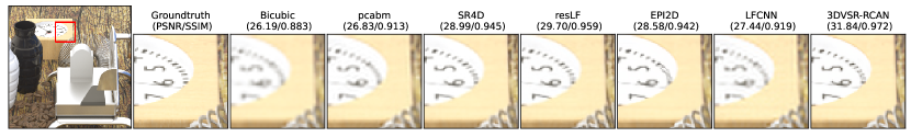
Figure 7: Qualitative comparison of SSR approaches on two scaling factors (${\mkern-2.0mu\times\mkern-2.0mu}2,{\mkern-2.0mu\times\mkern-2.0mu}4$). The SAI at $\boldsymbol{\theta}\!=\!(4,4)$ is visualized together with its zoom-in region marked by a red rectangle. The first two rows: ${\mkern-2.0mu\times\mkern-2.0mu}2$ results of synthetic scene coffee_beans_vases [10] and real-world scene general_55 [12]. The last two rows: ${\mkern-2.0mu\times\mkern-2.0mu}4$ results of synthetic scene smiling_crowd [10] and real-world scene ISO_Chart [14].

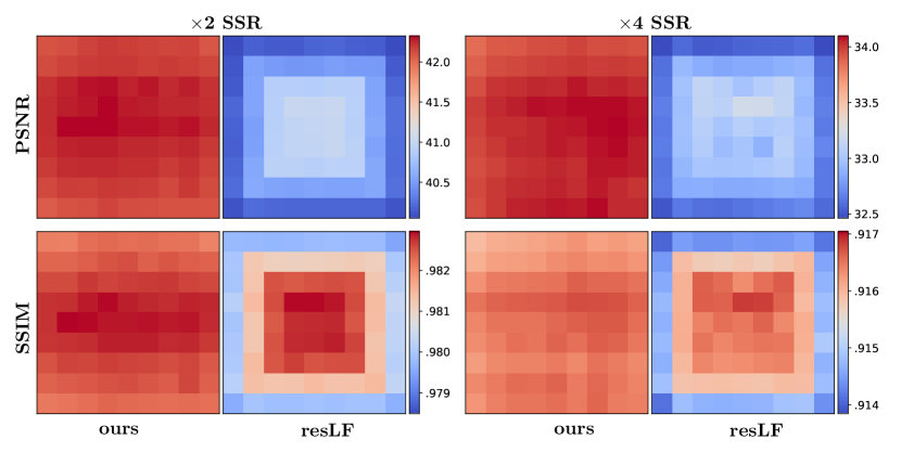
Figure 8: Visualization of PSNR and SSIM values on each SAI of light field scene two_vases [10]. Compared to ResLF [23], the proposed approach achieve a better reconstruction quality while maintaining a consistent performance on all perspective images.

In this section, the evaluation results of 3DVSR applied for SSR problem are discussed. We employed EDSR [15] and RCAN [16] for preliminary spatial super-resolution and tested against two scaling factors $\contour[1]{black}{$\zeta$}_{\mathfrak{\textbf{x}}}\!=\!2$ and $\contour[1]{black}{$\zeta$}_{\mathfrak{\textbf{x}}}\!=\!4$. Nine state-of-the-art approaches are selected for quantitative and qualitative comparisons. Among them, there are three SISR approaches (EDSR [15], DBPN [17], RCAN [16]) and six approaches provided for 4D LF (pcabm [18], LFnet [20], LFCNN [19], EPI2D [21], SR4D [22], resLF [23]). The result of bicubic interpolation is presented as a baseline result. All methods, except LFCNN, EPI2D, and LFnet, were tested using their released codes and pre-trained models. For EPI2D and LFnet, since the authors did not publish their source codes, we followed their papers to implement the models. Although the source code of LFCNN is available, its pre-trained model is not provided. Therefore, we retrained LFCNN, as well as EPI2D and LFnet, using our training dataset.

Table 4 lists quantitative results for ${\mkern-2.0mu\times\mkern-2.0mu}2$ and ${\mkern-2.0mu\times\mkern-2.0mu}4$ in terms of PSNR and SSIM metrics. For each scene, the quality metrics are calculated as an average of $7{\mkern-2.0mu\times\mkern-2.0mu}7$ SAIs in the middle. These values are then averaged over the test dataset. The two configurations of PSSR using EDSR and RCAN are denoted as 3DVSR-EDSR and 3DVSR-RCAN respectively. It can be seen from the table that the proposed approach scores the best PSNR and SSIM value for both $\times 2$ and $\times 4$ problems on average. Compared to SISR approaches EDSR and RCAN, 3DVSR respectively improves the reconstruction quality by 3.87dB and 3.63dB for ${\mkern-2.0mu\times\mkern-2.0mu}2$ and 3.13dB and 2.67dB for ${\mkern-2.0mu\times\mkern-2.0mu}4$. This improvement pays a tribute to the proposed enhancement network (EVRN) which exploits EPI volume structure to correct the high-frequency information from the output of SISR. The advantage of using EPI volume is also evident when compared to the 2D EPI-based approach [21]. Using a similar SISR technique (i.e. EDSR), the proposed approach scores 1.96 dB and 1.4dB better on average for ${\mkern-2.0mu\times\mkern-2.0mu}2$ and ${\mkern-2.0mu\times\mkern-2.0mu}4$ respectively.

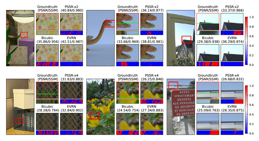
Figure 9: Comparison of two stages in reconstruction of spatially high resolution LF. The SAI at $\boldsymbol{\theta}\!=\!(4,4)$ is visualized together with its zoom-in region marked by a red rectangle. For each approach, an EPI at horizontal line marked in green is extracted and compared to the EPI of Groundtruth. The first row, from left to right: ${\mkern-2.0mu\times\mkern-2.0mu}2$ results of synthetic scene mona [8] and real-world scenes Ankylosaurus_&_Diplodocus_1, Framed [14]. The second row, from left to right: ${\mkern-2.0mu\times\mkern-2.0mu}4$ results of synthetic scene boxes [9] and real-world scenes Flowers, Sign [14].

Qualitative comparisons of six light field SSR approaches are shown in Fig. 7. It can be observed from the figures that the proposed approach shows superior performance in visual effects for both synthetic and real-world scenes. For example, only 3DVSR can reconstruct a correct pattern of wooden sticks in general_55 and clear detail of two faces in Smilling_crowd. In pcabm [18], the low-resolution light field image is divided into sets of patches that are then super-resolved separately. Although the overlapping of patches helps to smooth the output images, the inconsistencies in reconstruction quality between patches are unavoidable and lead to blocky artifacts (i.e. ISO_Chart, Smilling_crowd). In LFCNN [19], each SAI is super-resoluted independently using a SISR approach [41] whose CNN is quite trivial and shallow. LFCNN’s results are, therefore, over-smoothed in all the test scenes. SR4D [22] and resLF [23] include multiple SAIs in their super-resolution process. This allows them to exploit external information to reconstruct high-resolution images. However, these approaches still fail to reconstruct high quality images in challenging light field scenes with noisy and high-frequency pattern (i.e. general_55) or highly degraded content (i.e., ${\mkern-2.0mu\times\mkern-2.0mu}4$ down-sampled: ISO_Chart and Smilling_crowd). From the figure, their results are ambiguous and with obvious artifacts. Compared to EPI2D, we follow a similar approach in which the output of SISR is enhanced by reinforcing EPI structures of light field images. However, instead of relying on a narrow and feature-limited EPI as in EPI2D, we proposed to refine an EPI volume that allows us to exploit global information across multiple EPIs. Our results, therefore, show significantly better image qualities where the texture is recovered correctly and with more high-frequency details.

To investigate the reconstruction quality concerning different perspectives, we conducted an experiment in which the scene two_vases is used as input to perform both $\times 2$ and $\times 4$ SSR. For each view, the PSNR and SSIM values are computed, and the results are visualized in Fig. 8. Here, we compared our results with the results of state-of-the-art approach ResLF [23]. resLF employs a star-like structure of SAIs as input to super-resolute a single SAI lying in the center. This strategy is indeed beneficial to reconstruct high-resolution images. As in Table 4, resLF surpasses EPI2D and SR4D for most of the test dataset. However, the disadvantage of resLF’s approach is unequal treatment of SAI from different perspectives. For example, the SAI closed to the border has fewer input images than the SAI closed to the center. Therefore, reconstruction qualities of non-central views are relatively lower. In contrast, the proposed approach jointly uses EPI information and spatial information to reconstruct an EPI volume and thus achieves much higher output qualities with more stable distribution across all perspectives.

Fig. 9 presents a quantitative and qualitative comparison of EPI volumes reconstructed after the first stage (PSSR) and the second stage (EVRN). To better justify the improvement in angular dimension, we extract EPI images for each output and compare them to the EPI of the ground truth. From the figure, it is evident that the EVRN substantially improves the quality of reconstructed volume in both spatial and angular dimensions.

Table 5: Quantitative comparison of ASR approaches on 7 light field datasets

Approach	HCI17[9]	HCI13[8]	InLytro[13]	InSyn[10]	EPFL[14]	StGantry[11]	StLytro[12]	avg
nvs-mean	29.23/0.878	42.25/0.987	40.35/0.979	27.73/0.828	37.81/0.975	25.53/0.728	40.35/0.981	34.75/0.908
nvs-cnn	37.02/0.971	44.15/0.992	40.49/0.975	38.76/0.979	37.89/0.974	30.02/0.847	40.75/0.980	38.44/0.960
vsyn[26]	23.34/0.665	29.41/0.764	32.03/0.899	21.40/0.613	27.76/0.794	19.35/0.542	30.34/0.887	26.23/0.738
LFSR[27]	-/-	-/-	39.91/0.980	-/-	37.63/0.979	22.24/0.688	39.57/0.977	34.84/0.906
LFCNN[19]	30.97/0.883	38.78/0.967	35.36/0.948	29.09/0.834	34.43/0.949	26.01/0.739	36.41/0.957	33.01/0.897
Wang18[28]	31.66/0.893	41.74/0.984	37.31/0.967	29.36/0.831	36.18/0.969	27.04/0.741	38.86/0.971	34.59/0.908
Wu19[29]	29.93/0.917	30.76/0.832	33.73/0.922	28.67/0.871	29.48/0.843	20.80/0.631	32.45/0.937	29.40/0.850
Wu19a[30]	33.19/0.936	43.28/0.985	39.90/0.969	32.12/0.899	37.68/0.966	27.51/0.746	40.03/0.973	36.24/0.925
3DVSR-mean	40.12/0.979	47.07/0.994	44.22/0.985	40.32/0.979	43.64/0.987	32.30/0.854	43.41/0.985	41.58/0.966
3DVSR-cnn	40.00/0.981	45.15/0.994	43.04/0.982	40.90/0.982	42.30/0.986	32.11/0.861	42.20/0.980	40.81/0.967

(red: best, blue: second best)

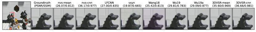
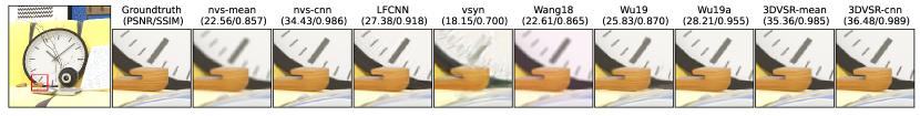
Figure 10: Qualitative comparison of ASR approaches on real-world and synthetic light field scenes. The SAI at $\boldsymbol{\theta}\!=\!(3,3)$ is visualized together with its zoom-in region marked by a red rectangle. The first two rows: real-world scenes lego [11] and flowers_plants_36 [12]. The last two rows: synthetic scenes big_clock [10] and sideboard [9].

5.4 Angular Super-Resolution

This section discusses the evaluation of the proposed approach for the angular super-resolution of light field images. The seven datasets listed in Table 1, are employed in this evaluation. For each scene in the test set, the angular resolution is down-sampled from $9{\mkern-2.0mu\times\mkern-2.0mu}9$ to $5{\mkern-2.0mu\times\mkern-2.0mu}5$ while the spatial resolution remains intact. With these low-resolution LFs as inputs, we then reconstruct the original size LFs follow the procedures discussed in Section 4. This means that 56 missed perspective images are reconstructed from 25 input images. In the PASR stage, we tested two approaches; one generates novel views by averaging, and the other using an end-to-end CNN. The results of these two PASR approaches and the final results after applying the refinement network are reported. We compare our approach with six previous approaches (vsyn [26], LFCNN [19], LFSR [27], Wang18 [28], Wu19 [29], and Wu19a [30]).

Table 5 lists quantitative results of ASR approaches running on the seven public datasets. We employed PSNR and SSIM as quality metrics that are computed for newly generated SAIs and are averaged over all scenes in each dataset. nvs-mean and nvs-cnn denotes the two PASR approaches. nvs-mean computes a novel perspective image by averaging two neighboring images, while nvs-cnn inferences a novel image using a residual CNN as depicted in Fig. 6. The outputs of nvs-mean and nvs-cnn enhanced by EVRN are denoted as 3DVSR-mean and 3DVSR-cnn respectively. LFSR [27] has a strict requirement of supported angular resolution. This approach employs a fully connected network in its output layer that always produces an angular-resolution of $14{\mkern-2.0mu\times\mkern-2.0mu}14$. For this reason, only real-world datasets [12, 13, 14, 11] are tested with this approach. From Table 5, it can be seen that the proposed approach provides the highest reconstruction quality. 3DVSR improves PSNR and SSIM values by a large margin as compared to the previous approaches (i.e., a minimum of 3dB improvement in all test datasets). In narrow-baseline light field images captured by a plenoptic camera [13, 14, 12], the difference between two neighboring views is almost invisible due to their sub-pixel displacement values (e.g., less than 0.5 pixel). In this case, a straightforward approach such as nvs-mean can score very well, and the benefit of employing CNN in the PASR stage is limited, i.e., the improvement of nvs-cnn over nvs-mean is smaller than 0.4dB. However, for the other test datasets, nvs-cnn presents a clear improvement compared to nvs-mean (i.e., 1.9dB to 7.8dB). By exploiting the EPI volume structure to refine the results of the PASR stage, 3DVSR achieves significant improvements over nvs-mean and nvs-cnn by an average of 6.8 dB and 2.4 dB, respectively. It is interesting to see that the performance of 3DVSR-mean is comparable to 3DVSR-cnn with a slightly better PSNR value (i.e., 0.7 dB). This demonstrates the superior performance of EVRN in reconstructing novel perspective images.

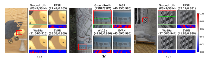
Figure 11: Comparison of two stages in reconstruction of angularly high resolution LF. The SAI at $\boldsymbol{\theta}\!=\!(3,3)$ is visualized together with its zoom-in region marked by a red rectangle. For each approach, an EPI at horizontal line marked in green is extracted and compared to the EPI of Groundtruth. From left to right: synthetic scene Flying_dice_dense [10], real-word scene general_29 [12], and synthetic scene bedroom [9].

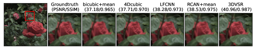
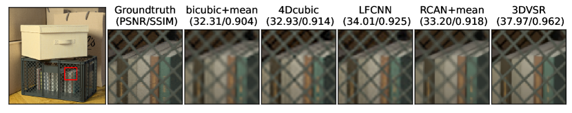
Figure 12: Angular-spatial super-resolution results of different approaches. The SAI at $\boldsymbol{\theta}\!=\!(3,3)$ is visualized together with its zoom-in region marked by a red rectangle. top row: real-world scene Rose  [13]; bottom row: synthetic scene boxes [8];

Fig. 10 shows the visual comparisons of evaluated ASR approaches on synthetic and real-world light field scenes. vsyn [26] consists of two CNNs; one predicts auxiliary disparity maps, and the other synthesizes novel views. It assumes that the disparity values of input light fields fall within a range that is quantized by a fixed step size. Based on the quantized disparity values, a cost volume is computed and is used as an input to the first CNN. The output disparity maps from the first CNN are used to pre-compute novel views that are then refined by the second CNN. The quality of the novel views highly depends on the accuracy of estimated disparity maps which are in turn depends on the cost volume and assumed disparity range. From the figure, it can be seen that vsync does not generalize well and performs poorly on light field scenes with a large disparity range (i.e., lego, big_clock, sideboard). Although the visual quality of the plenoptic scene (i.e., flowers_plants_36), for which vsyn was trained, is much better, it still suffers from the over-smoothed effect. Wang18 [28] employ a 3D CNN to recover the high-frequency detail of a stack of SAIs. Since their network architecture is relatively shallow and straightforward, it performs not so well and leaves a visible blurry effect on the synthesized images. Taking advantage of EPI structure, Wu19 [29] and Wu19a [30] can reconstruct images with more detail than Wang18. Both LFCNN and our cnn-based PASR approach (nvs-cnn) follow a similar strategy in which novel perspective images are synthesized by using their surrounding neighbor images. However, as opposed to the simple architecture of LFCNN, which only consists of convolution layers and activation layers, nvs-cnn employed many effective deep learning structures (i.e., global/local residual learning, dense connection). nvs-cnn, therefore, outperforms LFCNN with much better visual quality. Compared to nvs-cnn, the novel perspective images generated by nvs-mean are more ambiguous with over-smoothed regions and artifacts as the result of the averaging method. However, after being refined by EVRN the visual qualities of these images are significantly enhanced (i.e., 3DVSR-mean) and are comparable to the enhanced version of nvs-cnn (i.e., 3DVSR-cnn).

Fig. 11 compares the angular super-resolution results of Wu19a [30] and the proposed approaches after the first stage (PASR) and after the second stage (EVRN). In this experiment, nvs-mean is employed as a preliminary angular super-resolution approach, and the output volume of PASR is fed to EVRN for the final enhancement. Compared to our PASR, Wu19a provides a better reconstruction quality with sharper content and less angular error. However, the refined volume of EVRN is by far better than the output of Wu19a. As a result, we achieve a minimum of 3.3dB improvement in PSNR and less error in EPIs.

5.5 Angular-Spatial Super-resolution

In the ASSR problem, the resolution of 4D light field images is super-resoluted angularly and spatially. In other words, it consists of a super-resolution of each given SAI and a synthesis of novel perspective images which have the same higher resolution. As discussed in Section 4, the proposed approach handle ASSR in two stages. The first stage consists of PSSR followed by PASR to generate a 4D light field with the desired resolution. EVRN then enhances this preliminary up-sampled light field in the second stage to acquire the final output. To evaluate the proposed approach, we conducted an experiment in which the spatial scaling factor was set to $\contour[1]{black}{$\zeta$}_{\mathfrak{\textbf{x}}}=2$ and a similar ASR configuration as in Section 5.5 was applied.

The spatial-angular super-resolution results are shown in Fig. 12. bicubic+mean denotes a baseline approach that employs bicubic interpolation for SSR and averages neighbor views to generate novel perspective images. 4Dcubic denotes an approach in which cubic interpolation is applied on two spatial and two angular dimensions. RCAN+mean denotes the result of our preliminary stage which uses RCAN [16] for PSSR and nvs-mean for PASR. The result after an enhancement using EVRN is denoted as 3DVSR. Compared to the baseline approach and 4Dcubic, LFCNN provides a small improvement in reconstruction quality. Although LFCNN achieves an increase of about 1dB, its improvement in visual quality is negligible. The results of LFCNN are still ambiguous and lack high-frequency information. A similar performance can be seen in the results of RCAN+mean which are mostly over-smoothed due to the effect of averaging views. Compared to these approaches, 3DVSR produces a significant improvement in PSNR value (i.e., a minimum of 2.4 dB and 3.9 dB in scenes Rose and boxes respectively) and an obvious enhancement in visual quality.

6 Conclusion

This paper presents an angular-spatial light field super-resolution approach being able to reconstruct high-quality 4D light fields. Based on EPI volume structure, a 3D projected version of a 4D light field, we proposed a 2-stage framework that effectively addresses various problems in light field super-resolution, i.e., ASR, SSR, and ASSR. While the earlier stage provides flexible options to up-sample the input volume to the desired resolution, the later stage, which consists of an EPI volume-based enhancement CNN, substantially improves the reconstruction quality of the high-resolution EPI volume. The proposed enhancement network built on 3D convolutional operations and efficient deep learning structures, i.e., global/local residual learning, dense connection, multi-path learning, and attention-based scaling, effectively combines angular and spatial information from the 3D EPI volume structure to reconstruct high-frequency details. An extensive evaluation on 90 challenging synthetic and real-world light field scenes from 7 published datasets shows that the proposed approach outperforms state-of-the-art methods to a large extend for both spatial and angular super-resolution problems, i.e., an average PSNR improvement of more than 2.0 dB, 1.4 dB, and 3.14 dB in SSR ${\mkern-2.0mu\times\mkern-2.0mu}2$, SSR ${\mkern-2.0mu\times\mkern-2.0mu}4$, and ASR respectively. The reconstructed 4D light field demonstrates a balanced performance distribution across all perspective images and presents superior visual quality compared to the previous works.

References

- [1] G. Wu, B. Masia, A. Jarabo, Y. Zhang, L. Wang, Q. Dai, T. Chai, Y. Liu, Light field image processing: An overview, IEEE J. Sel. Topics Signal Process. 11 (7) (2017) 926–954. doi:10.1109/JSTSP.2017.2747126.
- [2] B. Wilburn, N. Joshi, V. Vaish, E.-V. Talvala, E. Antunez, A. Barth, A. Adams, M. Horowitz, M. Levoy, High performance imaging using large camera arrays, in: ACM Trans. Graph., Vol. 24, ACM, 2005, pp. 765–776.
- [3] J. Unger, A. Wenger, T. Hawkins, A. Gardner, P. Debevec, Capturing and rendering with incident light fields, Tech. rep., Inst. Creative Technology, Univ. Southern California (2003).
- [4] E. H. Adelson, J. Y. A. Wang, Single lens stereo with a plenoptic camera, IEEE Trans. Pattern Anal. Mach. Intell. (2) (1992) 99–106.
- [5] R. Ng, M. Levoy, M. Brédif, G. Duval, M. Horowitz, P. Hanrahan, Others, Light field photography with a hand-held plenoptic camera, Comput. Sci. Tech. Rep. CSTR 2 (11) (2005) 1–11.
- [6] A. Lumsdaine, T. Georgiev, The focused plenoptic camera, in: IEEE Int. Conf. Image Process., IEEE, 2009, pp. 1–8.
- [7] Z. Cheng, Z. Xiong, C. Chen, D. Liu, Light field super-resolution : A benchmark, in: CVPR Work., 2019.
- [8] S. Wanner, S. Meister, B. Goldlucke, Datasets and benchmarks for densely sampled 4d light fields, in: VMV 2013 Vis. Model. Vis., 2013, pp. 225–226.
- [9] K. Honauer, O. Johannsen, D. Kondermann, B. Goldluecke, A dataset and evaluation methodology for depth estimation on 4d light fields, Lect. Notes Comput. Sci. 10113 LNCS (2017) 19–34. doi:10.1007/978-3-319-54187-7_2.
- [10] J. Shi, X. Jiang, C. Guillemot, A framework for learning depth from a flexible subset of dense and sparse light field views (2019) 5867–5880doi:10.1109/TIP.2019.2923323.
-
[11]
Light fields from the lego
gantry, accessed: Feb. 2020.
URL http://lightfield.stanford.edu/lfs.html -
[12]
Stanford lytro light field
archive, accessed: Feb. 2020.
URL http://lightfields.stanford.edu/LF2016.html -
[13]
Lytro illum
light field dataset, accessed: Feb. 2020.
URL https://www.irisa.fr/temics/demos/IllumDatasetLF/index.html - [14] M. Rerabek, T. Ebrahimi, New light field image dataset, in: 8th International Conference on Quality of Multimedia Experience (QoMEX), no. CONF, 2016.
- [15] B. Lim, S. Son, H. Kim, S. Nah, K. M. Lee, Enhanced deep residual networks for single image super-resolution, in: IEEE Conf. Comput. Vis. Pattern Recognit. Work., 2017. arXiv:1707.02921.
- [16] Y. Zhang, K. Li, K. Li, L. Wang, B. Zhong, Y. Fu, Image super-resolution using very deep residual channel attention networks, in: ECCV, 2018.
- [17] M. Haris, G. Shakhnarovich, N. Ukita, Deep back-projection networks for super-resolution, in: IEEE Conf. Comput. Vis. Pattern Recognit., 2018, pp. 1664–1673. doi:10.1109/CVPR.2018.00179.
- [18] R. A. Farrugia, C. Galea, C. Guillemot, Super resolution of light field images using linear subspace projection of patch-volumes, IEEE J. Sel. Top. Signal Process. 11 (7) (2017) 1058–1071. doi:10.1109/JSTSP.2017.2747127.
- [19] Y. Yoon, H. G. Jeon, D. Yoo, J. Y. Lee, I. S. Kweon, Light-field image super-resolution using convolutional neural network, IEEE Signal Process. Lett. 24 (6) (2017) 848–852. doi:10.1109/LSP.2017.2669333.
- [20] Y. Wang, F. Liu, K. Zhang, G. Hou, Z. Sun, T. Tan, Lfnet: A novel bidirectional recurrent convolutional neural network for light-field image super-resolution, IEEE Trans. Image Process. 27 (9) (2018) 4274–4286. doi:10.1109/TIP.2018.2834819.
- [21] Y. Yuan, Z. Cao, L. Su, Light-field image superresolution using a combined deep cnn based on epi, IEEE Signal Process. Lett. 25 (9) (2018) 1359–1363. doi:10.1109/LSP.2018.2856619.
- [22] H. W. F. Yeung, J. Hou, X. Chen, J. Chen, Z. Chen, Y. Y. Chung, Light field spatial super-resolution using deep efficient spatial-angular separable convolution 28 (5) (2019) 2319–2330. doi:10.1109/TIP.2018.2885236.
- [23] S. Zhang, Y. Lin, H. Sheng, Residual networks for light field image super-resolution, IEEE Conf. Comput. Vis. Pattern Recognit. (2019) 11046–11055.
- [24] J. Kim, J. K. Lee, K. M. Lee, Accurate image super-resolution using very deep convolutional networks, in: 2016 IEEE Conf. Comput. Vis. Pattern Recognit., IEEE, 2016, pp. 1646–1654. doi:10.1109/CVPR.2016.182.
- [25] Y. Zhang, Y. Tian, Y. Kong, B. Zhong, Y. Fu, Residual dense network for image super-resolution, in: Proceedings of the IEEE Conference on Computer Vision and Pattern Recognition (CVPR), 2018.
- [26] N. K. Kalantari, T.-C. Wang, R. Ramamoorthi, Learning-based view synthesis for light field cameras, ACM Transactions on Graphics (Proceedings of SIGGRAPH Asia 2016) 35 (6) (2016).
- [27] M. S. K. Gul, B. K. Gunturk, Spatial and angular resolution enhancement of light fields using convolutional neural networks, IEEE Trans. Image Process. 27 (5) (2018) 2146–2159.
- [28] Y. Wang, F. Liu, Z. Wang, G. Hou, Z. Sun, T. Tan, End-to-end view synthesis for light field imaging with pseudo 4dcnn, in: Proceedings of the European Conference on Computer Vision (ECCV), 2018.
- [29] G. Wu, Y. Liu, Q. Dai, T. Chai, Learning sheared epi structure for light field reconstruction, IEEE Transactions on Image Processing 28 (7) (2019) 3261–3273. doi:10.1109/TIP.2019.2895463.
- [30] G. Wu, Y. Liu, L. Fang, Q. Dai, T. Chai, Light field reconstruction using convolutional network on epi and extended applications, IEEE Transactions on Pattern Analysis and Machine Intelligence 41 (7) (2019) 1681–1694. doi:10.1109/TPAMI.2018.2845393.
- [31] S. Heber, W. Yu, T. Pock, Neural epi-volume networks for shape from light field, in: IEEE Int. Conf. Comput. Vis., 2017, pp. 2271–2279. doi:10.1109/ICCV.2017.247.
- [32] H. Fan, D. Liu, Z. Xiong, F. Wu, Two-stage convolutional neural network for light field super-resolution, in: 2017 IEEE Int. Conf. Image Process., IEEE, 2017, pp. 1167–1171. doi:10.1109/ICIP.2017.8296465.
- [33] K. Mitra, A. Veeraraghavan, Light field denoising, light field superresolution and stereo camera based refocussing using a gmm light field patch prior, in: IEEE Conf. Comp. Vis. Pattern Recognit. Work., 2012, pp. 22–28. doi:10.1109/CVPRW.2012.6239346.
- [34] T. E. Bishop, P. Favaro, The light field camera: Extended depth of field, aliasing, and superresolution 34 (5) (2012) 972–986. doi:10.1109/TPAMI.2011.168.
- [35] M. Alain, A. Smolic, Light field super-resolution via lfbm5d sparse coding, in: IEEE Int. Conf. Image Process., 2018, pp. 2501–2505. doi:10.1109/ICIP.2018.8451162.
- [36] M. Rossi, M. E. Gheche, P. Frossard, A nonsmooth graph-based approach to light field super-resolution, in: IEEE Int. Conf. Image Process., 2018, pp. 2590–2594. doi:10.1109/ICIP.2018.8451127.
- [37] S. Wanner, B. Goldluecke, Variational light field analysis for disparity estimation and super-resolution, IEEE Trans. Pattern Anal. Mach. Intell. 36 (3) (2014) 606–619.
- [38] T. H. Tran, G. Mammadov, K. Sun, S. Simon, Gpu-accelerated light-field image super-resolution, in: Int. Conf. Adv. Comput. Appl., 2018, pp. 7–13. doi:10.1109/ACOMP.2018.00010.
- [39] M. Rossi, P. Frossard, Geometry-consistent light field super-resolution via graph-based regularization 27 (9) (2018) 4207–4218.
- [40] Y. Yoon, H.-G. Jeon, D. Yoo, J.-Y. Lee, I. So Kweon, Learning a deep convolutional network for light-field image super-resolution, in: IEEE Int. Conf. Comput. Vis. Work., 2015.
- [41] C. Dong, C. C. Loy, K. He, X. Tang, Learning a deep convolutional network for image super-resolution, in: European conference on computer vision, Springer, 2014, pp. 184–199.
- [42] M. Levoy, P. Hanrahan, Light field rendering, in: ACM Proc. 23rd Annu. Conf. Comput. Graph. Interact. Tech., 1996, pp. 31–42.
- [43] S. J. Gortler, R. Grzeszczuk, R. Szeliski, M. F. Cohen, The lumigraph, SIGGRAPH, (1996) 43–54doi:10.1145/237170.237200.
- [44] G. Huang, Z. Liu, L. Van Der Maaten, K. Q. Weinberger, Densely connected convolutional networks, in: IEEE Conf. Comput. Vis. Pattern Recognit., 2017, pp. 2261–2269.
- [45] S. Woo, J. Park, J.-Y. Lee, I. So Kweon, Cbam: Convolutional block attention module, in: The European Conf. Comput. Vis., 2018.
- [46] I. Loshchilov, F. Hutter, Decoupled weight decay regularization, in: Int. Conf. Learning Representations, 2019.