An algebraic attack to the Bluetooth stream cipher E0

Abstract.

In this paper we study the security of the Bluetooth stream cipher E0 from the viewpoint it is a “difference stream cipher”, that is, it is defined by a system of explicit difference equations over the finite field ${\mathrm{GF}}(2)$. This approach highlights some issues of the Bluetooth encryption such as the invertibility of its state transition map, a special set of 14 bits of its 132-bit state which when guessed implies linear equations among the other bits and finally a small number of spurious keys, with 83 guessed bits, which are compatible with a keystream of about 60 bits. Exploiting these issues, we implement an algebraic attack using Gröbner bases, SAT solvers and Binary Decision Diagrams. Testing activities suggest that the version based on Gröbner bases is the best one and it is able to attack E0 in about $2^{79}$ seconds on an Intel i9 CPU. To the best of our knowledge, this work improves any previous attack based on a short keystream, hence fitting with Bluetooth specifications.

1. Introduction

The Bluetooth protocol [6] is one of the most important players in the “wireless revolution” of consumer electronics. This communication protocol has started in 1999 in the mobile phones market and now it is present in almost all mobiles, personal computers, wireless headset and speakers, remote controllers and many other devices. Recently, the pandemic crisis has involved Bluetooth as an excellent tool to trace close proximity contacts. Bluetooth is a secure protocol which relies its privacy on the E0 stream cipher. This cipher consists of four independent Linear Feedback Shift Registers which are combined by means of a non-linear Finite State Machine.

By assuming a “known-plaintext attack”, the cryptanalysis of a stream cipher is generally based on the knowledge of some amount of bits of its keystream (see, for instance, [20, 25]). Following the introduction of the Bluetooth protocol, a number of cryptanalytic results has been obtained that can be essentially divided into two main classes: long or short keystream attacks. Indeed, an attack is generally faster when providing a large number of keystream bits (see, for instance, [2, 12, 15]) but this is actually forbidden by the Bluetooth design which has the payload of each frame associated to a single key consisting of only 2745 bits. According to this, the cryptanalysis of E0 in the present paper is based on a very short keystream containing about 60 bits. Note that in addition to these data, we essentially assume the knowledge of 83 bits of a 132-bit internal state of E0 by brute force. To determine the remaining bits is very fast by Gröbner bases computations which lead to a total running time for our attack of approximately $2^{79}$ seconds.

Another main distinction in the attacks to Bluetooth encryption is that some of them are correlations attacks as in [24] but one has also algebraic cryptanalysis [4]. In the class of algebraic attacks to E0 or similar stream ciphers, the most common approach involves Binary Decision Diagrams (briefly BDDs) as in [21, 22, 27, 28] and just few papers considered other solvers of polynomial systems as Gröbner bases and XL-algorithm [1, 3, 8]. The cryptanalysis we propose is based on Gröbner bases which show to be feasible solvers for polynomials systems having a few number of solutions. Indeed, the stream cipher E0 tends to have few keys that are compatible with a small number of keystream bits and this can be considered a possible flaw.

By means of a complete implementation of the proposed method, we compare the performance of Gröbner bases with SAT solvers and BDDs using a large test set. Another practical algebraic attack to E0 one has in the literature is the BDD-based attack described in [27]. Our Gröbner bases timings are much better than the runtimes we obtain for SAT solvers and BDDs where the latter ones confirm and improve the timings in [27].

Note that Bluetooth protocol implements a reinitialization of the initial state of E0 using the last 128 keystream bits obtained by clocking the cipher 200 times. Since our algebraic attack can be performed using less than 128 keystream bits, a double initialization can be recovered simply by applying the attack twice.

The paper is structured as follows. In Section 2 we explain how to solve a polynomial system with coefficients and solutions in a finite field by means of a guess-and-determine strategy, that is, by using the exhaustive evaluation over the finite field of a subset of variables and Gröbner bases as solvers of the remaining variables. We explain that this method is feasible especially when the system has a single or few solutions. In Section 3 we review and expand the theory of difference stream ciphers that has been recently introduced in [18] to cryptanalyze stream and block ciphers. In particular, we show that the invertibility property of the explicit difference system governing the evolution of the internal state of a difference stream cipher is a possible issue for its security. Moreover, we study methods to eliminate the variables of this explicit difference system in order to speed-up an algebraic attack to the keys that are consistent with a given keystream.

In Section 4 we describe the Bluetooth stream cipher E0 and in Section 5 and 6 we show that it is an invertible difference stream cipher by providing its explicit difference equations together with the ones of its inverse system. In Section 6 we explain how cryptanalytic methods for difference stream ciphers are applied in our attack to the Bluetooth encryption. In Section 7 we present the choice of the 83 variables that are brute forced in the guess-and-determine strategy and we explain how 14 of them have been single out by the difference stream cipher structure of E0 in order to speed-up the Gröbner bases computations.

In Section 8 we present a complete statistics of our practical algebraic attack to E0 by comparing Gröbner bases with SAT solvers and BDDs. The test set we use are $2^{17}$ random evaluations of the 83 variables for $2^{3}$ different keys. The testing activity clearly shows that Gröbner bases perform better than the other solvers with a total running time of about $2^{79}$ seconds with an Intel i9 processor. To the best of our knowledge, the complexity $2^{83}$ also improves any previous attack with short keystreams (see, for instance, [20, 27]). A full cryptanalysis of E0, including its double initialization trick, it is therefore available with complexity $2^{84}$. We end the paper with Section 9 where some conclusions are drawn.

2. Guess-and-determine strategy

In algebraic cryptanalysis, to attack a stream, block or public key cipher essentially consists in solving a system of polynomial equations over a finite field ${\mathbb{K}}={\mathrm{GF}}(q)$ which has generally a single or few ${\mathbb{K}}$-solutions. Indeed, this assumption is a natural one if a reasonable amount of data as plaintexts, ciphertexts, keystreams and so on, is available for the attack and few keys are compatible with such data. To fix notations, let $r,n>0$ be two integers and consider the polynomial system

(1) $$\left\{\begin{array}[]{ccc}f_{1}&=&0\\ \vdots&&\vdots\\ f_{n}&=&0\\ \end{array}\right.$$

where $f_{i}\in P={\mathbb{K}}[x_{1},\ldots,x_{r}]$, for all $1\leq i\leq n$. Denote by $J=\langle f_{1},\ldots,f_{n}\rangle$ the ideal of $P$ generated by the polynomials $f_{i}$ and consider

$$L=\langle x_{1}^{q}-x_{1},\ldots,x_{r}^{q}-x_{r}\rangle\subset P.$$

The generators of the ideal $L$ are called “field equations” because of the following well-known result (see, for instance, [14]).

Proposition 2.1.

Let $\bar{{\mathbb{K}}}$ be the algebraic closure of ${\mathbb{K}}$ and denote

$$V(J)=\{(\alpha_{1},\ldots,\alpha_{r})\in\bar{{\mathbb{K}}}^{r}\mid f_{i}(\alpha_{1},\ldots,\alpha_{r})=0\ (1\leq i\leq n)\}.$$

Put $V_{\mathbb{K}}(J)=V(J)\cap{\mathbb{K}}^{r}$ and call $V_{\mathbb{K}}(J)$ the set of the ${\mathbb{K}}$-solutions of $J$, that is, of the polynomial system (1). We have that $V(L)={\mathbb{K}}^{r}$ and $V_{\mathbb{K}}(J)=V(J+L)$ where $J+L\subset P$ is a radical ideal.

An immediate upper bound to the complexity of computing $V_{\mathbb{K}}(J)$ is clearly

$$\lambda=q^{r}$$

by assuming that the evaluation of all polynomials $f_{i}$ over a vector $(\beta_{1},\ldots,\beta_{r})\in{\mathbb{K}}^{r}$ is performed in unit time. If ${\mathbb{K}}={\mathrm{GF}}(2)$, we have that SAT solvers may slightly improve such complexity for special systems (see, for instance, [4], Paragraph 13.4.2.1). Applications of the SAT solving to boolean polynomial systems arising in cryptography are found, for example, in [7, 10, 26]. Another approach to polynomial system solving is symbolic computation, that is, to compute consequences of the equations of the system (1) which allow to obtain easily its solutions. A suitable method consists in computing a Gröbner basis (see, for instance, [16, 23]) of the ideal $J=\langle f_{1},\ldots,f_{n}\rangle\subset P$. Indeed, by the Nullstellensatz Theorem for finite fields (see [14]) one obtains the following result.

Proposition 2.2.

Assume that the polynomial system $(\ref{sys})$ has a single or no ${\mathbb{K}}$-solution. Then, the (reduced) universal Gröbner basis $G$ of the ideal $J+L$, that is, its Gröbner basis with respect to any monomial ordering of $P$ is

$$G=\left\{\begin{array}[]{cl}\{x_{1}-\alpha_{1},\ldots,x_{r}-\alpha_{r}\}&\mbox{if}\ V_{\mathbb{K}}(J)=\{(\alpha_{1},\ldots,\alpha_{r})\},\\ \{1\}&\mbox{otherwise}.\end{array}\right.$$

Observe that Gröbner bases have generally bad exponential complexity with respect to the number of variables $r$ which is even worse than brute force complexity $\lambda=q^{r}$ (see, for instance, [4], Section 12.2). Nevertheless, if the number of variables $r$ is moderate and the polynomial system $(\ref{sys})$ has few ${\mathbb{K}}$-solutions then Gröbner bases (in general symbolic computation) become an effective tool for solving it. Indeed, by Proposition 2.2 we can choose most efficient monomial orderings as DegRevLex to solve the system. Moreover, when there are no solutions and the Gröbner basis is simply $G=\{1\}$ then the Buchberger algorithm is stopped once a constant in ${\mathbb{K}}$ is obtained as an element of the current basis, say $H$. If there is a single solution, another optimization consists in stopping the algorithm once each variable $x_{i}$ ($1\leq i\leq r$) is obtained as the leading monomial of an element in $H$.

In the case $V_{\mathbb{K}}(J)$ consists of few ${\mathbb{K}}$-solutions, note that the cost of obtaining them is again essentially that of computing a DegRevLex-Gröbner basis of $J+L$. In fact, for solving one needs to convert this basis into a Lex-Gröbner basis by means of the FGLM-algorithm [11] which has complexity ${\mathcal{O}}(rd^{3})$ where $d=\#V_{\mathbb{K}}(J)=\dim_{\mathbb{K}}P/(J+L)$. If the integer $d$ is small, such complexity is dominated by the cost of computing the DegRevLex-Gröbner basis.

To simplify notations and statements, from now on we assume that the polynomial system (1) has a single ${\mathbb{K}}$-solution, that is, $V_{\mathbb{K}}(J)=\{(\alpha_{1},\ldots,\alpha_{r})\}$. A standard way to reduce the complexity of solving a polynomial system with a large number of variables consists in solving equivalently many systems having less variables that are obtained by evaluating some subset of variables, say $\{x_{1},\ldots,x_{s}\}$ ($0\leq s\leq r$), in all possible ways over the finite field ${\mathbb{K}}$. In other words, for all vectors $(\beta_{1},\ldots,\beta_{s})\in{\mathbb{K}}^{s}$ one defines the linear ideal

$$E_{\beta_{1},\ldots,\beta_{s}}=\langle x_{1}-\beta_{1},\ldots,x_{s}-\beta_{s}\rangle\subset P$$

and consider the corresponding ideal

$$J_{\beta_{1},\ldots,\beta_{s}}=J+L+E_{\beta_{1},\ldots,\beta_{s}}.$$

Moreover, we denote by

$$\begin{gathered}H_{\beta_{1},\ldots,\beta_{s}}=\{f_{1}(\beta_{1},\ldots,\beta_{s},x_{s+1},\ldots,x_{r}),\ldots,f_{n}(\beta_{1},\ldots,\beta_{s},x_{s+1},\ldots,x_{r}),\\ x_{s+1}^{q}-x_{s+1},\ldots,x_{r}^{q}-x_{r},x_{1}-\beta_{1},\ldots,x_{s}-\beta_{s}\}\subset P\end{gathered}$$

the generating set of $J_{\beta_{1},\ldots,\beta_{s}}$ and we assume that $H_{\beta_{1},\ldots,\beta_{s}}$ can be computed in a negligible time. One has clearly that

$$V(J_{\beta_{1},\ldots,\beta_{s}})=\left\{\begin{array}[]{cl}\{(\alpha_{1},\ldots,\alpha_{r})\}&\mbox{if}\ (\beta_{1},\ldots,\beta_{s})=(\alpha_{1},\ldots,\alpha_{s}),\\ \emptyset&\mbox{otherwise}.\end{array}\right.$$

This approach is generally called a guess-and-determine $($or hybrid [5]$)$ strategy which has sequential running time

$$\mu_{s}=\sum_{(\beta_{1},\ldots,\beta_{s})\in{\mathbb{K}}^{s}}\tau_{\beta_{1},\ldots,\beta_{s}}$$

where $\tau_{\beta_{1},\ldots,\beta_{s}}$ is the time for computing a DegRevLex-Gröbner basis of $J_{\beta_{1},\ldots,\beta_{s}}$ starting with the generating set $H_{\beta_{1},\ldots,\beta_{s}}$. Denote by $\tau_{s}$ the average runtime of such a computation, that is

$$\tau_{s}=(\sum\tau_{\beta_{1},\ldots,\beta_{s}})/q^{s}.$$

For a sufficiently large number $0\leq s\leq r$ of evaluated variables, one has generally that $\tau_{s}\leq q^{r-s}$, that is, the total running time $\mu_{s}=q^{s}\tau_{s}$ of a guess-and-determine strategy improves the brute force complexity. This motivates the use of Gröbner bases. An optimization of this strategy is achieved for a choice of the subset of variables $\{x_{1},\ldots,x_{s}\}$ such that $\mu_{s}$ is minimal. Obviously, if $r$ is a large number of variables the search for this optimal choice may be not a trivial task.

Observe that for all $q^{s}-1$ vectors $(\beta_{1},\ldots,\beta_{s})\neq(\alpha_{1},\ldots,\alpha_{s})$ the computed Gröbner basis is always $G=\{1\}$, that is, the average computing time $\tau_{s}$ is essentially obtained for inconsistent polynomial systems where Gröbner bases behave generally better than SAT solvers. This is another motivation for using Gröbner bases in a guess-and-determine strategy. The superiority of Gröbner bases can be explained by observing that the UNSAT case is obtained by a SAT solver essentially by exploring the full space. On the other hand, a symbolic method proves the inconsistency of a system of equations by constructing some consequence of them of type $1=0$. For an experimental evidence of this, see for instance [18] and Section 8 of the present paper where we show that Gröbner bases perform better than SAT solver and Binary Decision Diagrams when attacking the stream cipher E0.

Note finally that if $V(J_{\beta_{1},\ldots,\beta_{s}})$ contains many solutions, one can determine their number without actually solving as

$$\#V(J_{\beta_{1},\ldots,\beta_{s}})=\dim_{\mathbb{K}}P/J_{\beta_{1},\ldots,\beta_{s}}.$$

This ${\mathbb{K}}$-dimension of the quotient algebra $P/J_{\beta_{1},\ldots,\beta_{s}}$ can be easily computed by means of a DegRevLex-Gröbner basis of the ideal $J_{\beta_{1},\ldots,\beta_{s}}$ (see, for instance, [16, 23]).

3. Difference stream ciphers

Aiming to apply a guess-and-determine strategy to the cryptanalysis of the Bluetooth stream cipher E0, we review briefly here the theory of difference stream ciphers and their algebraic attacks. Indeed, we will show in Section 5 that E0 is such a cipher. For all details we refer to the recent paper [18].

Let ${\mathbb{K}}$ be any field and fix an integer $n>0$. Consider a set of variables $X(t)=\{x_{1}(t),\ldots,x_{n}(t)\}$, for all integers $t\geq 0$ and put $X=\bigcup_{t\geq 0}X(t)$. For the corresponding polynomial algebra $R={\mathbb{K}}[X]$ we consider the algebra endomorphism $\sigma:R\to R$ such that $x_{i}(t)\mapsto x_{i}(t+1)$, for all $1\leq i\leq n$ and $t\geq 0$. The algebra $R$ under the action of $\sigma$ is called the algebra of (ordinary) difference polynomials. Fix now some integers $r_{1},\ldots,r_{n}\geq 0$ and define the subset

$${\bar{X}}=\{x_{1}(0),\ldots,x_{1}(r_{1}-1),\ldots,x_{n}(0),\ldots,x_{n}(r_{n}-1)\}\subset X.$$

We finally denote by ${\bar{R}}={\mathbb{K}}[{\bar{X}}]\subset R$ the corresponding subalgebra.

Definition 3.1.

Consider some polynomials $f_{1},\ldots,f_{n}\in{\bar{R}}$. A system of (algebraic ordinary) explicit difference equations is by definition an infinite system of polynomial equations of the kind

$$\left\{\begin{array}[]{ccc}x_{1}(r_{1}+t)&=&\sigma^{t}(f_{1}),\\ &\vdots\\ x_{n}(r_{n}+t)&=&\sigma^{t}(f_{n}).\\ \end{array}\right.\quad(t\geq 0)$$

over the infinite set of variables $X$. Such a system is denoted briefly as

(2) $$\left\{\begin{array}[]{ccc}x_{1}(r_{1})&=&f_{1},\\ &\vdots\\ x_{n}(r_{n})&=&f_{n}.\\ \end{array}\right.$$

An $n$-tuple of functions $(a_{1},\ldots,a_{n})$ where each $a_{i}:{\mathbb{N}}\to{\mathbb{K}}$ $(1\leq i\leq n)$ satisfies the above system is called a ${\mathbb{K}}$-solution of $(\ref{dsys})$. Put $r=r_{1}+\ldots+r_{n}$ and for all $t\geq 0$ define the vector

$$v(t)=(a_{1}(t),\ldots,a_{1}(t+r_{1}-1),\ldots,a_{n}(t),\ldots,a_{n}(t+r_{n}-1))\in{\mathbb{K}}^{r}.$$

We call $v(t)$ the $t$-state of the ${\mathbb{K}}$-solution $(a_{1},\ldots,a_{n})$. In particular, $v(0)$ is called its initial state.

Definition 3.2.

Consider an explicit difference system $(\ref{dsys})$. We define the algebra endomorphism ${\bar{\mathrm{T}}}:{\bar{R}}\to{\bar{R}}$ by putting, for any $i=1,2,\dots,n$

$$x_{i}(0)\mapsto x_{i}(1),\ldots,x_{i}(r_{i}-2)\mapsto x_{i}(r_{i}-1),x_{i}(r_{i}-1)\mapsto f_{i}.$$

If $r=r_{1}+\ldots+r_{n}$, we denote by ${\mathrm{T}}:{\mathbb{K}}^{r}\to{\mathbb{K}}^{r}$ the polynomial map corresponding to ${\mathrm{T}}$. In other words, if $v(t)$ is the $t$-state of a ${\mathbb{K}}$-solution $(a_{1},\ldots,a_{n})$ we have that ${\mathrm{T}}(v(t))=v(t+1)$, for all clocks $t\geq 0$. We call ${\bar{\mathrm{T}}}$ the state transition endomorphism and ${\mathrm{T}}$ the state transition map of the explicit difference system $(\ref{dsys})$.

Since $v(t)={\mathrm{T}}^{t}(v(0))$, it is clear that the ${\mathbb{K}}$-solutions $(a_{1},\ldots,a_{n})$ of (2) are in one-to-one correspondence with their initial states

$$v(0)=(a_{1}(0),\ldots,a_{1}(r_{1}-1),\ldots,a_{n}(0),\ldots,a_{n}(r_{n}-1)).$$

An important class of explicit difference systems are the ones such that for any $t\leq t^{\prime}$ we can compute a $t$-state by the knowledge of a $t^{\prime}$-state.

Definition 3.3.

Consider the state transition endomorphism ${\bar{\mathrm{T}}}:{\bar{R}}\to{\bar{R}}$ and the corresponding state transition map ${\mathrm{T}}:{\mathbb{K}}^{r}\to{\mathbb{K}}^{r}$ of an explicit difference system $(\ref{dsys})$. We call the system invertible if ${\bar{\mathrm{T}}}$ is an automorphism. In this case, ${\mathrm{T}}$ is also a bijective map.

An invertibility criterion for endomorphisms of polynomial algebras can be obtained in terms of symbolic computation and Gröbner bases. For a comprehensive reference we refer to the book [30].

Theorem 3.4.

Let $X=\{x_{1},\ldots,x_{r}\},X^{\prime}=\{x^{\prime}_{1},\ldots,x^{\prime}_{r}\}$ be two disjoint variable sets and define the polynomial algebras $P={\mathbb{K}}[X],P^{\prime}={\mathbb{K}}[X^{\prime}]$ and $Q={\mathbb{K}}[X\cup X^{\prime}]=P\otimes P^{\prime}$. Consider an algebra endomorphism $\varphi:P\to P$ such that $x_{1}\mapsto g_{1},\ldots,x_{r}\mapsto g_{r}$ $(g_{i}\in P)$ and the corresponding ideal $J\subset Q$ which is generated by the set $\{x^{\prime}_{1}-g_{1},\ldots,x^{\prime}_{r}-g_{r}\}$. Moreover, we endow the polynomial algebra $Q$ by a product monomial ordering such that $X\succ X^{\prime}$. Then, the map $\varphi$ is an automorphism of $P$ if and only if the reduced Gröbner basis of $J$ is of the kind $\{x_{1}-g^{\prime}_{1},\ldots,x_{r}-g^{\prime}_{r}\}$ where $g^{\prime}_{i}\in P^{\prime}$, for all $1\leq i\leq r$. In this case, if $\varphi^{\prime}:P^{\prime}\to P^{\prime}$ is the algebra endomorphism such that $x^{\prime}_{1}\mapsto g^{\prime}_{1},\ldots,x^{\prime}_{r}\mapsto g^{\prime}_{r}$ and $\xi:P\to P^{\prime}$ is the isomorphism $x_{1}\mapsto x^{\prime}_{1},\ldots,x_{r}\mapsto x^{\prime}_{r}$, we have that $\xi\,\varphi^{-1}=\varphi^{\prime}\,\xi$.

Based on the above result, we introduce the following notion for invertible systems.

Definition 3.5.

Denote ${\bar{R}}^{\prime}={\mathbb{K}}[{\bar{X}}^{\prime}]$ where

$${\bar{X}}^{\prime}=\{x^{\prime}_{1}(0),\ldots,x^{\prime}_{1}(r_{1}-1),\ldots,x^{\prime}_{n}(0),\ldots,x^{\prime}_{n}(r_{n}-1)\}$$

and put $Q={\mathbb{K}}[{\bar{X}}\cup{\bar{X}}^{\prime}]={\bar{R}}\otimes{\bar{R}}^{\prime}$. Consider an invertible system $(\ref{dsys})$ and the corresponding ideal $J\subset Q$ which is generated by the following polynomials, for any $i=1,2,\ldots,n$

$$x^{\prime}_{i}(0)-x_{i}(1),\ldots,x^{\prime}_{i}(r_{i}-2)-x_{i}(r_{i}-1),x^{\prime}_{i}(r_{i}-1)-f_{i}.$$

Assume that $Q$ is endowed with a product monomial ordering such that ${\bar{X}}\succ{\bar{X}}^{\prime}$ and let

$$G=\bigcup_{i}\{x_{i}(1)-x^{\prime}_{i}(0),\ldots,x_{i}(r_{i}-1)-x^{\prime}_{i}(r_{i}-2),x_{i}(0)-f^{\prime}_{i}\}$$

be the reduced Gröbner basis of $J$. Denote by $g_{i}$ the image of $f^{\prime}_{i}$ under the algebra isomorphism ${\bar{R}}^{\prime}\to{\bar{R}}$ such that, for any $i=1,2,\ldots,n$

$$x^{\prime}_{i}(0)\mapsto x_{i}(r_{i}-1),x^{\prime}_{i}(1)\mapsto x_{i}(r_{i}-2),\ldots x^{\prime}_{i}(r_{i}-1)\mapsto x_{i}(0).$$

The inverse of an invertible system $(\ref{dsys})$ is by definition the following explicit difference system

(3) $$\left\{\begin{array}[]{ccc}x_{1}(r_{1})&=&g_{1},\\ &\vdots\\ x_{n}(r_{n})&=&g_{n}.\\ \end{array}\right.$$

The following results are proved in [18].

Proposition 3.6.

Let ${\bar{\mathrm{T}}},{\bar{\mathrm{S}}}:{\bar{R}}\to{\bar{R}}$ be the state transition automorphisms of an invertible system (2) and its inverse system (3), respectively. Denote by $\xi:{\bar{R}}\to{\bar{R}}$ the algebra automorphism such that

$$x_{i}(0)\mapsto x_{i}(r_{i}-1),x_{i}(1)\mapsto x_{i}(r_{i}-2),\ldots,x_{i}(r_{i}-1)\mapsto x_{i}(0).$$

One has that $\xi{\bar{\mathrm{S}}}={\bar{\mathrm{T}}}^{-1}\xi$.

By the above proposition we obtain immediately the following result explaining how to practically reverse the evolution of the state of an invertible system by using the corresponding inverse system.

Proposition 3.7.

Let $(\ref{invdsys})$ be the inverse system of an invertible system $(\ref{dsys})$. If $(a_{1},\ldots,a_{n})$ is a ${\mathbb{K}}$-solution of $(\ref{dsys})$, consider its $t$-state $(t\geq 0)$

$$v=(a_{1}(t),\ldots,a_{1}(t+r_{1}-1),\ldots,a_{n}(t),\ldots,a_{n}(t+r_{n}-1)).$$

Denote by $(b_{1},\ldots,b_{n})$ the ${\mathbb{K}}$-solution of $(\ref{invdsys})$ whose initial state is

$$v^{\prime}=(a_{1}(t+r_{1}-1),\ldots,a_{1}(t),\ldots,a_{n}(t+r_{n}-1),\ldots,a_{n}(t)).$$

If the $t$-state of $(b_{1},\ldots,b_{n})$ is

$$u^{\prime}=(b_{1}(t),\ldots,b_{1}(t+r_{1}-1),\ldots,b_{n}(t),\ldots,b_{n}(t+r_{n}-1)),$$

then the initial state of $(a_{1},\ldots,a_{n})$ is

$$u=(b_{1}(t+r_{1}-1),\ldots,b_{1}(t),\ldots,b_{n}(t+r_{n}-1),\ldots,b_{n}(t)).$$

From now on, we will assume that ${\mathbb{K}}={\mathrm{GF}}(q)$ is a finite field.

Definition 3.8.

A difference stream cipher ${\mathcal{C}}$ is by definition an explicit difference system $(\ref{dsys})$ together with a polynomial $f\in{\bar{R}}$. Let $(a_{1},\ldots,a_{n})$ be a ${\mathbb{K}}$-solution of $(\ref{dsys})$ and denote as usual by $v(t)\in{\mathbb{K}}^{r}$ $(r=r_{1}+\ldots+r_{n})$ its $t$-state. The initial state $v(0)$ is called the key of the ${\mathbb{K}}$-solution $(a_{1},\ldots,a_{n})$ and the function $b:{\mathbb{N}}\to{\mathbb{K}}$ such that $b(t)=f(v(t))$ for all $t\geq 0$, is called the keystream of $(a_{1},\ldots,a_{n})$. We call $f$ the keystream polynomial of the cipher ${\mathcal{C}}$. Finally, the cipher ${\mathcal{C}}$ is said invertible if such is the system $(\ref{dsys})$.

A “known-plaintext attack” to a stream cipher essentially implies the knowledge of the keystream as the difference between the known ciphertext and plaintext streams. Indeed, the keystream is usually provided after a sufficiently high number of clocks in order to prevent cryptanalysis. This motivates the following notion.

Definition 3.9.

Let ${\mathcal{C}}$ be a difference stream cipher consisting of the system $(\ref{dsys})$ and the keystream polynomial $f$. Let $b:{\mathbb{N}}\to{\mathbb{K}}$ be the keystream of a ${\mathbb{K}}$-solution of $(\ref{dsys})$ and fix a clock $T\geq 0$. Consider the ideal

$$J=\sum_{t\geq T}\,\langle\sigma^{t}(f)-b(t)\rangle\subset R$$

and denote by $V_{\mathbb{K}}(J)$ the set of the ${\mathbb{K}}$-solutions of $J$. An algebraic attack to ${\mathcal{C}}$ by the keystream $b$ after $T$ clocks consists in computing the ${\mathbb{K}}$-solutions $(a_{1},\ldots,a_{n})$ of the system $(\ref{dsys})$ such that $(a_{1},\ldots,a_{n})\in V_{\mathbb{K}}(J)$. In other words, by considering the ideal corresponding to $(\ref{dsys})$, that is

$$I=\sum_{t\geq 0}\,\langle x_{1}(r_{1}+t)-\sigma^{t}(f_{1}),\ldots,x_{n}(r_{n}+t)-\sigma^{t}(f_{n})\rangle\subset R$$

we want to compute $V_{\mathbb{K}}(I+J)=V_{\mathbb{K}}(I)\cap V_{\mathbb{K}}(J)$.

Since the given function $b$ is the keystream of a ${\mathbb{K}}$-solution of (2), say $(a_{1},\ldots,a_{n})$, we have clearly that $(a_{1},\ldots,a_{n})\in V_{\mathbb{K}}(I+J)\neq\emptyset$. For actual ciphers, we have generally that $V_{\mathbb{K}}(I+J)=\{(a_{1},\ldots,a_{n})\}$. We will assume such a unique solution from now on.

In practice, a finite number of values of the keystream $b$ is actually provided in algebraic attacks. In other words, for a fixed integer bound $B\geq T$, we consider the polynomial algebra $R_{B}={\mathbb{K}}[X_{B}]$ over the finite variable set $X_{B}=\bigcup_{0\leq t\leq B}X(t)$ and the ideals $I_{B},J_{B}\subset R_{B}$ whose finite generating sets are respectively

$$\begin{gathered}\{x_{i}(r_{i}+t)-\sigma^{t}(f_{i})\in R_{B}\mid 1\leq i\leq n,t\geq 0\},\\ \{\sigma^{t}(f)-b(t)\in R_{B}\mid t\geq T\}.\end{gathered}$$

It is shown in [18] that for a sufficiently large bound $B$, the uniqueness of the ${\mathbb{K}}$-solution is preserved and we have that

$$V_{\mathbb{K}}(I_{B}+J_{B})=\{(a^{\prime}_{1},\ldots,a^{\prime}_{n})\}$$

where each function $a^{\prime}_{i}:\{0,\ldots,B\}\to{\mathbb{K}}$ ($1\leq i\leq n$) is such that $a^{\prime}_{i}(t)=a_{i}(t)$ for all $0\leq t\leq B$. Since ${\mathbb{K}}$-solutions are in one-to-one correspondence with their initial states that are the keys of a difference stream cipher, this means that we can perform an actual algebraic attack without obtaining any spurious, that is, incorrect key once a sufficiently large number of keystream values is provided.

If the explicit difference system (2) is invertible we can essentially assume that the initial keystream clock is $T=0$. In fact, by means of the notion of inverse system in Definition 3.5 the computation of the $T$-state is completely equivalent to the computation of the initial state, that is, the key. Moreover, if we consider the ideal

$$J^{\prime}=\sum_{t\geq 0}\,\langle\sigma^{t}(f)-b(T+t)\rangle\subset R$$

we have that the initial states of the ${\mathbb{K}}$-solutions in $V_{\mathbb{K}}(I+J^{\prime})$ are exactly the $T$-states of the ${\mathbb{K}}$-solutions in $V_{\mathbb{K}}(I+J)$. By putting $B^{\prime}=B-T$, an algebraic attack to an invertible difference stream cipher is therefore reduced to the computation of $V_{\mathbb{K}}(I_{B^{\prime}}+J^{\prime}_{B^{\prime}})$. Since $T$ is generally an high value of clock, for invertible ciphers this is a very effective optimization of the algebraic cryptanalysis because this trick reduces drastically the number of variables to solve. Indeed, instead of solving equations in the polynomial algebra $R_{B}$ ($0\leq T\leq B$) we can solve equivalent equations in $R_{B^{\prime}}$ ($B^{\prime}=B-T$).

Another possible option to reduce the number of variables may consist in eliminating all variables except for the initial variables, that is, the variables of the set ${\bar{X}}$ by means of the explicit difference equations of the system (2). In this way one obtains the equations satisfied by the keys of a difference stream cipher having a given keystream. To explain this, we introduce the following notions (see also [13, 17]).

Definition 3.10.

A commutative algebra $A$ together with an algebra endomorphism $\alpha:A\to A$ is called a difference algebra. An ideal $J\subset A$ such that $\alpha(J)\subset J$ is said a difference ideal. Let $(A,\alpha),(B,\beta)$ be two difference algebras. An algebra homomorphism $\varphi:A\to B$ is called a difference algebra homomorphism if $\varphi\alpha=\beta\varphi$.

Note that the kernel of a difference algebra homomorphism is clearly a difference ideal. In our context, we consider the difference algebras $(R,\sigma)$ and $({\bar{R}},{\bar{\mathrm{T}}})$. The ideal $I=\sum_{t\geq 0}\,\langle x_{1}(r_{1}+t)-\sigma^{t}(f_{1}),\ldots,x_{n}(r_{n}+t)-\sigma^{t}(f_{n})\rangle$ is a difference ideal of $R$. We denote hence $I=\langle x_{1}(r_{1})-f_{1},\ldots,x_{n}(r_{n})-f_{n}\rangle_{\sigma}$ to mean that the set $\{x_{1}(r_{1})-f_{1},\ldots,x_{n}(r_{n})-f_{n}\}$ generates $I$ as a difference ideal.

Theorem 3.11.

Let $\varphi:R\to{\bar{R}}$ be the algebra homomorphism such that its restriction to ${\bar{R}}$ is the identity map and for all $t\geq 0$ one has that

$$x_{i}(r_{i}+t)\mapsto{\bar{\mathrm{T}}}^{t}(f_{i})\ (1\leq i\leq n).$$

It holds that $\varphi$ is a difference algebra homomorphism and its kernel is $I=\ker\varphi$.

Proof.

Since $\varphi$ is an algebra homomorphism, it is sufficient to show that the property $\varphi\sigma={\bar{\mathrm{T}}}\varphi$ holds over the variables. For the variables $x_{i}(0),\ldots,x_{i}(r_{i}-2)$ ($1\leq i\leq n$) this is trivial since the actions of $\sigma,{\bar{\mathrm{T}}}$ coincide and the restriction of $\varphi$ to ${\bar{R}}$ is the identity map. Moreover, we have

$$\varphi(\sigma(x_{i}(r_{i}-1))=\varphi(x_{i}(r_{i}))=f_{i}={\bar{\mathrm{T}}}(x_{i}(r_{i}-1))={\bar{\mathrm{T}}}(\varphi(x_{i}(r_{i}-1))).$$

In the same way, for all $t>0$ one has

$$\varphi(\sigma(x_{i}(r_{i}-1+t))=\varphi(x_{i}(r_{i}+t))={\bar{\mathrm{T}}}^{t}(f_{i})={\bar{\mathrm{T}}}{\bar{\mathrm{T}}}^{t-1}(f_{i})={\bar{\mathrm{T}}}(\varphi(x_{i}(r_{i}-1+t))).$$

We show now that ${\mathrm{Ker\,}}\varphi=I$. Since $I=\langle x_{1}(r_{1})-f_{1},\ldots,x_{n}(r_{n})-f_{n}\rangle_{\sigma}$ and $\varphi(x_{i}(r_{i})-f_{i})=f_{i}-f_{i}=0$, we have that $I\subset{\mathrm{Ker\,}}\varphi$.

Consider now a polynomial $f\in R$. By means of the identities $x_{i}(r_{i}+t)\equiv\sigma^{t}(f_{i})$ modulo $I$ ($1\leq i\leq n,t\geq 0$) we have that $f\equiv\bar{f}$ modulo $I$, for some polynomial $\bar{f}\in{\bar{R}}$. Assume now that $f\in{\mathrm{Ker\,}}\varphi$. Since $I\subset{\mathrm{Ker\,}}\varphi$, we have that $\bar{f}\in{\mathrm{Ker\,}}\varphi$. Because the restriction of $\varphi$ to ${\bar{R}}$ is the identity map, we have that $\bar{f}=0$ and hence $f\in I$. ∎

Denote by $\sigma^{\prime}:R/I\to R/I$ the algebra endomorphism which is induced by $\sigma:R\to R$ since $\sigma(I)\subset I$. By the above result we obtain immediately the following one.

Corollary 3.12.

The difference algebras $(R/I,\sigma^{\prime})$ and $({\bar{R}},{\bar{\mathrm{T}}})$ are isomorphic by means of the difference algebra isomorphism $\varphi^{\prime}:R/I\to{\bar{R}}$ which is induced by $\varphi$.

In terms of bijective polynomial maps corresponding to algebra isomorphisms, the above result can be restated in the following way.

Proposition 3.13.

Consider $V_{\mathbb{K}}(I)$ the set of all ${\mathbb{K}}$-solutions of $(\ref{dsys})$. The map $\iota:V_{\mathbb{K}}(I)\to{\mathbb{K}}^{r}$ $(r=r_{1}+\ldots+r_{n})$ such that

$$(a_{1},\ldots,a_{n})\mapsto(a_{1}(0),\ldots,a_{1}(r_{1}-1),\ldots,a_{n}(0),\ldots,a_{n}(r_{n}-1))$$

is bijective and $\iota,\iota^{-1}$ are both polynomial maps.

From the above result we obtain that the set of keys that are compatible with the given keystream $b$, that is, $\iota(V_{\mathbb{K}}(I+J))$ is indeed the set of the ${\mathbb{K}}$-solutions of some polynomial system in ${\bar{R}}$. In other words, we have that $\iota(V_{\mathbb{K}}(I+J))=V_{\mathbb{K}}({\bar{J}})$ for some ideal ${\bar{J}}\subset{\bar{R}}$. We look for a generating set of ${\bar{J}}$.

Proposition 3.14.

We have that

$${\bar{J}}=\sum_{t\geq T}\langle{\bar{\mathrm{T}}}^{t}(f)-b(t)\rangle.$$

Proof.

Since $f\in{\bar{R}}$, it is sufficient to observe that the polynomial $\sigma^{t}(f)$ maps to ${\bar{\mathrm{T}}}^{t}(f)$ under the difference algebra homomorphism $\varphi$. ∎

A possible problem with the equations satisfied by the keys compatible with a given keystream is that they could have a very high degree if the explicit difference system $(\ref{dsys})$ is non-linear. To avoid this problem, one can perform a partial elimination only with the lowest degree equations of the system $(\ref{dsys})$. We make use of this approach when attacking the cipher E0 in the next sections since its explicit difference system contains linear equations, that is, LFSRs. We formalize this partial elimination approach by the following results which are a straightforward generalization of the previous ones.

Fix an integer $0\leq m\leq n$. Denote

$$\begin{gathered}{\bar{X}}^{\prime}_{m}=\{x_{1}(0),\ldots,x_{1}(r_{1}-1),\ldots,x_{m}(0),\ldots,x_{m}(r_{m}-1)\},\\ {\bar{X}}^{\prime\prime}_{m}=\bigcup_{t\geq 0}\{x_{m+1}(t),\ldots,x_{n}(t)\}\end{gathered}$$

and put ${\bar{X}}_{m}={\bar{X}}^{\prime}_{m}\cup{\bar{X}}^{\prime\prime}_{m}\subset X$. Denote by ${\bar{R}}_{m}={\mathbb{K}}[{\bar{X}}_{m}]\subset R$ the corresponding subalgebra. We define the endomorphism ${\bar{\mathrm{T}}}_{m}:{\bar{R}}_{m}\to{\bar{R}}_{m}$ such that

$$\begin{gathered}x_{i}(0)\mapsto x_{i}(1),\ldots,x_{i}(r_{i}-2)\mapsto x_{i}(r_{i}-1),x_{i}(r_{i}-1)\mapsto f_{i}\ (1\leq i\leq m),\\ x_{i}(t)\mapsto x_{i}(t+1)\ (m+1\leq i\leq n).\end{gathered}$$

We have clearly that ${\bar{\mathrm{T}}}_{0}=\sigma$ and ${\bar{\mathrm{T}}}_{n}={\bar{\mathrm{T}}}$. Define the ideal ${\bar{I}}_{m}\subset{\bar{R}}_{m}$ such that

$${\bar{I}}_{m}=\sum_{t\geq 0}\langle x_{m+1}(r_{m+1}+t)-{\bar{\mathrm{T}}}_{m}^{t}(f_{m+1}),\ldots,x_{n}(r_{n}+t)-{\bar{\mathrm{T}}}_{m}^{t}(f_{n})\rangle.$$

Note that ${\bar{\mathrm{T}}}_{m}({\bar{I}}_{m})\subset{\bar{I}}_{m}$ and ${\bar{I}}_{m}=\langle x_{m+1}(r_{m+1})-f_{m+1},\ldots,x_{n}(r_{n})-f_{n}\rangle_{{\bar{\mathrm{T}}}_{m}}$. Denote by ${\bar{\mathrm{T}}}^{\prime}_{m}:{\bar{R}}_{m}/{\bar{I}}_{m}\to{\bar{R}}_{m}/{\bar{I}}_{m}$ the algebra endomorphism which is induced by ${\bar{\mathrm{T}}}_{m}:{\bar{R}}_{m}\to{\bar{R}}_{m}$.

Theorem 3.15.

Let $\varphi_{m}:R\to{\bar{R}}_{m}$ be the algebra homomorphism such that its restriction to ${\bar{R}}_{m}$ is the identity map and for all $t\geq 0$ one has that

$$x_{i}(r_{i}+t)\mapsto{\bar{\mathrm{T}}}_{m}^{t}(f_{i})\ (1\leq i\leq m).$$

It holds that $\varphi_{m}$ is a difference algebra homomorphism and its kernel is $I=\ker\varphi_{m}$.

Corollary 3.16.

The difference algebras $(R/I,\sigma^{\prime})$ and $({\bar{R}}_{m}/{\bar{I}}_{m},{\bar{\mathrm{T}}}^{\prime}_{m})$ are isomorphic by means of the difference algebra isomorphism $\varphi^{\prime}_{m}:R/I\to{\bar{R}}_{m}/{\bar{I}}_{m}$ which is induced by $\varphi_{m}$.

In terms of corresponding polynomial maps, we have the following result.

Proposition 3.17.

Consider $V_{\mathbb{K}}({\bar{I}}_{m})$ the set of all ${\mathbb{K}}$-solutions of the system of polynomial equations

$$\left\{\begin{array}[]{rcl}x_{m+1}(r_{m+1}+t)&=&{\bar{\mathrm{T}}}_{m}^{t}(f_{m+1})\\ &\vdots\\ x_{n}(r_{n}+t)&=&{\bar{\mathrm{T}}}_{m}^{t}(f_{n})\\ \end{array}\right.\quad(t\geq 0)$$

over the set of variables ${\bar{X}}_{m}$. The map $\iota_{m}:V_{\mathbb{K}}(I)\to V_{\mathbb{K}}({\bar{I}}_{m})$ such that

$$(a_{1},\ldots,a_{n})\mapsto(a_{1}(0),\ldots,a_{1}(r_{1}-1),\ldots,a_{m}(0),\ldots,a_{m}(r_{n}-1),a_{m+1},\ldots,a_{n})$$

is bijective and $\iota_{m},\iota_{m}^{-1}$ are both polynomial maps.

Proposition 3.18.

We have that $\iota_{m}(V_{\mathbb{K}}(I+J))=V_{\mathbb{K}}({\bar{I}}_{m}+{\bar{J}}_{m})$ where

$${\bar{J}}_{m}=\sum_{t\geq T}\langle{\bar{\mathrm{T}}}_{m}^{t}(f)-b(t)\rangle\subset{\bar{R}}_{m}$$

Note that actual computations with the ideal ${\bar{J}}_{m}$ are done by assuming that $T\leq t\leq B$ for a sufficiently large bound $B\geq T$. Moreover, for an invertible cipher we always assume that $T=0$.

Finally, it is useful to observe the following. Suppose that $R$ is endowed with a monomial ordering $\succ$ such that, for all $t\geq 0$

$$x_{i}(r_{i}+t)\succ\sigma^{t}(f_{i})\ (1\leq i\leq m).$$

In this case, for any polynomial $g\in{\bar{R}}_{m}$ we can compute ${\bar{\mathrm{T}}}_{m}^{t}(g)$ in an alternative way. Consider the ideal

$$\begin{gathered}I_{m}=\sum_{t\geq 0}\langle x_{1}(r_{1}+t)-\sigma^{t}(f_{1}),\ldots,x_{m}(r_{m}+t)-\sigma^{t}(f_{m})\rangle\\ =\langle x_{1}(r_{1})-f_{1},\ldots,x_{m}(r_{m})-f_{m}\rangle_{\sigma}\subset R\end{gathered}$$

whose generating set is a Gröbner basis because its leading monomials are distinct linear ones. We have that ${\bar{\mathrm{T}}}_{m}^{t}(g)$ is indeed the normal form of the polynomial $g$ modulo $I_{m}$ with respect to the given monomial ordering. For more details, see [18].

4. The stream cipher E0

From now on, we assume that the finite base field is ${\mathbb{K}}={\mathrm{GF}}(2)={\mathbb{Z}}_{2}$. In order to avoid confusion, in the present section we denote by $\mathop{\dot{+}}$ the sum in ${\mathbb{Z}}$ and by $+$ the sum in ${\mathbb{K}}$. The Bluetooth stream cipher E0 is obtained by four Linear Feedback Shift Registers (briefly LFSRs) that are combined by a Finite State Machine (FSM) as described in Figure 1.

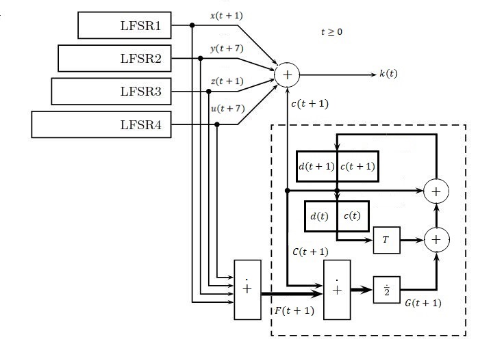
Figure 1. E0 Bluetooth Stream Cipher

The four LFSRs are respectively defined by the following primitive polynomials with coefficients in ${\mathbb{K}}$

$$\begin{array}[]{rcl}p_{1}&=&x^{25}+x^{17}+x^{13}+x^{5}+1,\\ p_{2}&=&x^{31}+x^{19}+x^{15}+x^{7}+1,\\ p_{3}&=&x^{33}+x^{29}+x^{9}+x^{5}+1,\\ p_{4}&=&x^{39}+x^{35}+x^{11}+x^{3}+1.\\ \end{array}$$

For all clocks $t\geq 0$, the state of the FSM consists of $4$ bits which are stored in a pair of 2-bit delay elements, say

$$(d(t),c(t)),(d(t+1),c(t+1))\in{\mathbb{K}}^{2}.$$

It is useful to define the corresponding integer numbers

$$\begin{gathered}C(t)=d(t)2\mathop{\dot{+}}c(t),\hskip 18.0pt\\ C(t+1)=d(t+1)2\mathop{\dot{+}}c(t+1).\end{gathered}$$

At any clock, the lower delay element stores the previous value of the upper element, that is, $(d(t+1),c(t+1))$ stores in $(d(t),c(t))$. Then, the new 2-bit $(d(t+2),c(t+2))$ for the upper delay element of the combiner is computed by putting

$$(d(t+2),c(t+2))=(g_{1}(t+1),g_{0}(t+1))+(d(t+1),c(t+1))+T(d(t),c(t))$$

where $T:{\mathbb{K}}^{2}\rightarrow{\mathbb{K}}^{2}$ is the linear bijection

$$(d(t),c(t))\mapsto(c(t),d(t)+c(t))$$

and the 2-bit $(g_{1}(t+1),g_{0}(t+1))\in{\mathbb{K}}^{2}$ is defined as follows. Consider the sum

$$F(t)=x(t)\mathop{\dot{+}}y(t+6)\mathop{\dot{+}}z(t)\mathop{\dot{+}}u(t+6)\in{\mathbb{Z}}$$

and define the integer

$$G(t+1)=\left\lfloor\frac{F(t+1)\mathop{\dot{+}}C(t+1)}{2}\right\rfloor.$$

Since $0\leq G(t+2)\leq 3$, we define the 2-bit element $(g_{1}(t+1),g_{0}(t+1))\in{\mathbb{K}}^{2}$ as the binary representation of $G(t+1)$, namely

$$G(t+1)=g_{1}(t+1)2\mathop{\dot{+}}g_{0}(t+1).$$

Finally, for all $t\geq 0$ the keystream bits of the cipher E0 are computed as the sum

$$k(t)=x(t+1)+y(t+7)+z(t+1)+u(t+7)+c(t+1)\in{\mathbb{K}}.$$

5. E0 is a difference stream cipher

We show now that we can obtain E0 as a difference stream cipher, that is, we can translate it into a system of difference equations. The four independent LFSRs correspond immediately to the following subsystem of linear difference equations

(4) $$\left\{\begin{array}[]{rcl}x(25)&=&x(0)+x(5)+x(13)+x(17),\\ y(31)&=&y(0)+y(7)+y(15)+y(19),\\ z(33)&=&z(0)+z(5)+z(9)+z(29),\\ u(39)&=&u(0)+u(3)+u(11)+u(35),\\ \end{array}\right.$$

Let us consider now the FSM combiner. Since $0\leq F(t)\leq 4$, the binary representation of $F(t)$ consists of a 3-bit element $(f_{2}(t),f_{1}(t),f_{0}(t))\in{\mathbb{K}}^{3}$, that is

$$F(t)=f_{2}(t)2^{2}\mathop{\dot{+}}f_{1}(t)2\mathop{\dot{+}}f_{0}(t).$$

Clearly, we can view $F(t)=x(t)\mathop{\dot{+}}y(t+6)\mathop{\dot{+}}z(t)\mathop{\dot{+}}u(t+6)$ as a function ${\mathbb{K}}^{4}\to{\mathbb{Z}}$ with variable set $\{x(t),y(t+6),z(t),u(t+6)\}$ and therefore $f_{0}(t),f_{1}(t),f_{2}(t)$ as Boolean functions ${\mathbb{K}}^{4}\to{\mathbb{K}}$ with the same variable set. By converting the latter functions into their Algebraic Normal Form (briefly ANF), that is, as elements of the polynomial algebra ${\mathbb{K}}[x(t),y(t+6),z(t),u(t+6)]$ modulo the identities

$$\begin{gathered}x(t)^{2}+x(t)=y(t+6)^{2}+y(t+6)=z(t)^{2}+z(t)=u(t+6)^{2}+u(t+6)=0\end{gathered}$$

we obtain that

$$\begin{array}[]{rcl}f_{0}(t)&=&x(t)+y(t+6)+z(t)+u(t+6),\\ f_{1}(t)&=&x(t)y(t+6)+x(t)z(t)+x(t)u(t+6)+y(t+6)z(t)\\ &&+\,y(t+6)u(t+6)+z(t)u(t+6),\\ f_{2}(t)&=&x(t)y(t+6)z(t)u(t+6).\end{array}$$

Standard methods to obtain the ANF involves Support and Minterm Representation of Boolean functions and we refer to the book [32] for all details about them.

We consider now the following sum of integers

$$F(t)\mathop{\dot{+}}C(t)=f_{2}(t)2^{2}\mathop{\dot{+}}f_{1}(t)2\mathop{\dot{+}}f_{0}(t)\mathop{\dot{+}}d(t)2\mathop{\dot{+}}c(t)$$

whose binary representation, as a result of carries, is

$$\begin{gathered}F(t)\mathop{\dot{+}}C(t)=(f_{2}(t)+f_{1}(t)d(t)+f_{0}(t)c(t)d(t)+f_{1}(t)f_{0}(t)c(t))2^{2}\\ \mathop{\dot{+}}\,(f_{0}(t)c(t)+f_{1}(t)+d(t))2\mathop{\dot{+}}(f_{0}(t)+c(t)).\end{gathered}$$

By dividing by 2, we obtain that

$$\begin{gathered}\frac{F(t)\mathop{\dot{+}}C(t)}{2}=(f_{2}(t)+f_{1}(t)d(t)+f_{0}(t)c(t)d(t)+f_{1}(t)f_{0}(t)c(t))2\\ \mathop{\dot{+}}\,(f_{0}(t)c(t)+f_{1}(t)+d(t))\mathop{\dot{+}}(f_{0}(t)+c(t))2^{-1}.\end{gathered}$$

and therefore it holds that

$$\begin{gathered}\left\lfloor\frac{F(t)\mathop{\dot{+}}C(t)}{2}\right\rfloor=(f_{2}(t)+f_{1}(t)d(t)+f_{0}(t)c(t)d(t)+f_{1}(t)f_{0}(t)c(t))2\\ \mathop{\dot{+}}\,(f_{0}(t)c(t)+f_{1}(t)+d(t)).\end{gathered}$$

Since, by definition, we have that

$$G(t+1)=g_{1}(t+1)2\mathop{\dot{+}}g_{0}(t+1)=\left\lfloor\frac{F(t+1)\mathop{\dot{+}}C(t+1)}{2}\right\rfloor$$

we conclude that

$$\begin{array}[]{rcl}g_{1}(t+1)&=&f_{2}(t+1)+f_{1}(t+1)d(t+1)+f_{0}(t+1)c(t+1)d(t+1)\\ &&+\,f_{1}(t+1)f_{0}(t+1)c(t+1),\\ g_{0}(t+1)&=&f_{0}(t+1)c(t+1)+f_{1}(t+1)+d(t+1).\\ \end{array}$$

Finally, by using the definition

$$(d(t+2),c(t+2))=(g_{1}(t+1),g_{0}(t+1))+(d(t+1),c(t+1))+(c(t),d(t)+c(t))$$

we obtain that

$$\begin{array}[]{rcl}d(t+2)&=&f_{2}(t+1)+f_{1}(t+1)d(t+1)+f_{0}(t+1)c(t+1)d(t+1)\\ &&+\,f_{1}(t+1)f_{0}(t+1)c(t+1)+d(t+1)+c(t),\\ c(t+2)&=&f_{0}(t+1)c(t+1)+f_{1}(t+1)+d(t+1)+c(t+1)+d(t)+c(t).\\ \end{array}$$

Define now the variable set

$$\begin{gathered}{\bar{X}}=\{x(0),\ldots,x(24),y(0),\ldots,x(30),z(0),\ldots,z(32),\\ u(0),\ldots,u(38),c(0),c(1),d(0),d(1)\}\end{gathered}$$

and the corresponding polynomial algebra ${\bar{R}}={\mathbb{K}}[{\bar{X}}]$. By the above calculations, we have that E0 is a difference stream cipher whose evolution of the internal state $v(t)\in{\mathbb{K}}^{132}$ ($t\geq 0$) is described by the following system of explicit difference equations

(5) $$\left\{\begin{array}[]{rcl}x(25)&=&x(0)+x(5)+x(13)+x(17),\\ y(31)&=&y(0)+y(7)+y(15)+y(19),\\ z(33)&=&z(0)+z(5)+z(9)+z(29),\\ u(39)&=&u(0)+u(3)+u(11)+u(35),\\ c(2)&=&g^{\prime}_{0},\\ d(2)&=&g^{\prime}_{1}\\ \end{array}\right.$$

where the non-linear polynomials $g^{\prime}_{0},g^{\prime}_{1}\in{\bar{R}}$ are defined as

$$\begin{array}[]{rcl}g^{\prime}_{0}&=&x(1)c(1)+y(7)c(1)+z(1)c(1)+u(7)c(1)+x(1)y(7)+x(1)z(1)\\ &&+\,x(1)u(7)+y(7)z(1)+y(7)u(7)+z(1)u(7)+c(1)+d(1)+c(0)+d(0),\\ g^{\prime}_{1}&=&x(1)y(7)z(1)u(7)+x(1)y(7)d(1)+x(1)z(1)d(1)+x(1)u(7)d(1)\\ &&+\,y(7)z(1)d(1)+y(7)u(7)d(1)+z(1)u(7)d(1)+x(1)c(1)d(1)\\ &&+\,y(7)c(1)d(1)+z(1)c(1)d(1)+u(7)c(1)d(1)+x(1)y(7)z(1)c(1)\\ &&+\,x(1)y(7)u(7)c(1)+x(1)z(1)u(7)c(1)+y(7)z(1)u(7)c(1)+d(1)+c(0).\\ \end{array}$$

Finally, the keystream polynomial $f\in{\bar{R}}$ of E0 is defined as

$$f=x(1)+y(7)+z(1)+u(7)+c(1).$$

In other words, for each clock $t\geq 0$ a keystream of E0 is obtained by evaluating the polynomial $f$ over the $t$-state $v(t)\in{\mathbb{K}}^{132}$ of a ${\mathbb{K}}$-solution of (5).

Note that Bluetooth specifications [6] require that the keystream outputs after a reinitialization at clock $T=200$. Finally, remark that our description of E0 matches with the sample data contained in Appendix IV of those specifications once all initial states of the LFSRs are reversed and one considers the initial state of the FSM as $(c(0),d(0),c(1),d(1))$. Indeed, the initial states of the non-linear equations of (5) are $(c(0),c(1))$ and $(d(0),d(1))$.

6. An algebraic attack to E0

As a result of Theorem 3.4 and Definition 3.5, we have that the explicit difference system (5) of E0 is invertible with inverse system

$$\left\{\begin{array}[]{rcl}x(25)&=&x(20)+x(12)+x(8)+x(0),\\ y(31)&=&y(24)+y(16)+y(12)+y(0),\\ z(33)&=&z(28)+z(24)+z(4)+z(0),\\ u(39)&=&u(36)+u(28)+u(4)+u(0),\\ c(2)&=&h_{0},\\ d(2)&=&h_{1}\\ \end{array}\right.$$

where the polynomials $h_{0},h_{1}\in{\bar{R}}$ are defined as

$$\begin{array}[]{rcl}h_{0}&=&x(24)y(24)z(32)u(32)+x(24)y(24)z(32)c(1)+x(24)y(24)u(32)c(1)\\ &&+\,x(24)z(32)u(32)c(1)+y(24)z(32)u(32)c(1)+x(24)y(24)d(1)\\ &&+\,x(24)z(32)d(1)+y(24)z(32)d(1)+x(24)u(32)d(1)+y(24)u(32)d(1)\\ &&+\,z(32)u(32)d(1)+x(24)c(1)d(1)+y(24)c(1)d(1)+z(32)c(1)d(1)\\ &&+u(32)c(1)d(1)+d(1)+d(0),\\ h_{1}&=&x(24)y(24)z(32)u(32)+x(24)y(24)z(32)c(1)+x(24)y(24)u(32)c(1)\\ &&+\,x(24)z(32)u(32)c(1)+y(24)z(32)u(32)c(1)+x(24)y(24)d(1)\\ &&+\,x(24)z(32)d(1)+y(24)z(32)d(1)+x(24)u(32)d(1)+y(24)u(32)d(1)\\ &&+\,z(32)u(32)d(1)+x(24)c(1)d(1)+y(24)c(1)d(1)+z(32)c(1)d(1)\\ &&+\,u(32)c(1)d(1)+x(24)y(24)+x(24)z(32)+y(24)z(32)+x(24)u(32)\\ &&+\,y(24)u(32)+z(32)u(32)+x(24)c(1)+y(24)c(1)+z(32)c(1)\\ &&+\,u(32)c(1)+c(1)+c(0)+d(0).\\ \end{array}$$

We recall that this inverse system is easily obtained by computing a suitable Gröbner basis. The invertibility of the system (5) allows us to attack equivalently any internal state. A convenient choice consists hence in attacking the state corresponding to the clock where the keystream starts to output.

With the notations of the Section 3, in our experiments we choose to compute $V_{\mathbb{K}}(I_{B}+J_{B})$ for a clock bound $B$ in the range $57\leq B\leq 69$, that is, we use for the attack the knowledge of a number $K$ of keystream bits in the range $51\leq K\leq 63$. To reduce the number of tests, we consider $K$ odd.

In this range we have found very few ${\mathbb{K}}$-solutions at each instance, in a suitably large test set, of a guess-and-determine strategy for solving $V_{\mathbb{K}}(I_{B}+J_{B})$. This strategy is based on the exhaustive evaluations of 83 variables and in the next section we explain how 14 of such variables have been chosen to speed-up the computations. The considered test set consists of $2^{17}$ evaluations for $2^{3}$ different keys.

For each guess of the 83 variables, we are able to determine the number of ${\mathbb{K}}$-solutions of the corresponding polynomial system as the ${\mathbb{K}}$-dimension of the quotient algebra modulo the ideal generated by the system and the field equations (see Section 2). Such dimension is easily obtained as a by-product of the DegRevLex-Gröbner basis that is computed at each evaluation.

These ${\mathbb{K}}$-solutions for wrong guesses of the 83 variables corresponds to spurious keys which can be detected by using some additional very small number of values of the keystream. Indeed, for $K=63$ the number of spurious keys for each guess is on the average close to zero. Note that a good trade-off consists in using a value of $K$ that lies approximately in the middle of the range $51\leq K\leq 63$ because the cost of solving grows significantly with $K$ but the cost of computing and comparing a few extra keystream bits is indeed very small.

Since the explicit difference system of E0 contains the combiner equations which are of degree 2 and 4, the approach we use to define the polynomial system to solve is the partial elimination described in Proposition 3.17 and Proposition 3.18. Namely, we perform elimination by the linear difference equations, that is, the LFSRs of the system $(\ref{e0sys})$. Once we fix a clock bound $B$, the corresponding polynomial system is defined over the following variable set

$$\begin{gathered}\{x(0),\ldots,x(24),y(0),\ldots,y(30),z(0),\ldots,z(32),\\ u(0),\ldots,u(38),c(0),\ldots,c(B),d(0),\ldots,d(B)\}.\end{gathered}$$

In our guess-and-determine strategy, a subset of 83 such variables are evaluated over the finite field ${\mathbb{K}}={\mathrm{GF}}(2)$ in an exhaustive way, leading to Gröbner bases computations that take few tens of milliseconds on the average.

We observe that other partial eliminations could be considered, including total elimination of all variables except for the initial ones that are

$$\begin{gathered}\{x(0),\ldots,x(24),y(0),\ldots,y(30),z(0),\ldots,z(32),\\ u(0),\ldots,u(38),c(0),c(1),d(0),d(1)\}.\end{gathered}$$

Indeed, we have experimented that all these variants increase the degree of the eliminated polynomials in a way that either makes them impossible to be computed or leads to polynomial systems which are more difficult to solve.

7. Fourteen useful variables

The set of the 83 evaluated variables that we have used to attack E0 by means of a guess-and-determine strategy applied to its difference stream cipher structure is the following one

$$\begin{gathered}\{x(0),\ldots,x(24),y(0),\ldots,y(26),y(29),z(0),\ldots,z(10),z(29),\ldots,z(32),\\ u(0),\ldots,u(9),u(35),u(36),u(37),c(0),d(0)\}.\end{gathered}$$

Fourteen of the above variables have been single out by means of the arguments in this section. The remaining 69 variables have been obtained by an experimental optimization.

The monomial ordering that we use for computing Gröbner bases and normal forms during the attack to E0 is defined as the DegRevLex-ordering over the following variable set

$$\begin{gathered}\{x(0),y(0),z(0),u(0),x(1),y(1),z(1),u(1),\ldots\}\\ \cup\,\{c(0),c(1),\ldots\}\cup\{d(0),d(1),\ldots\}\end{gathered}$$

induced by putting

$$\begin{gathered}x(0)\prec y(0)\prec z(0)\prec u(0)\prec x(1)\prec y(1)\prec z(1)\prec u(1)\prec\ldots\\ \prec c(0)\prec c(1)\prec\ldots\prec d(0)\prec d(1)\prec\ldots\end{gathered}$$

We consider the following polynomials which belong to the difference ideal $I$ corresponding to the explicit difference system $(\ref{e0sys})$

$$\begin{array}[]{rcl}C_{0}&=&c(2)+x(1)c(1)+y(7)c(1)+z(1)c(1)+u(7)c(1)+x(1)y(7)+x(1)z(1)\\ &&+\,x(1)u(7)+y(7)z(1)+y(7)u(7)+z(1)u(7)+c(1)+d(1)+c(0)+d(0),\\ C_{1}&=&c(3)+x(2)c(2)+y(8)c(2)+z(2)c(2)+u(8)c(2)+x(2)y(8)+x(2)z(2)\\ &&+\,x(2)u(8)+y(8)z(2)+y(8)u(8)+z(2)u(8)+c(2)+d(2)+c(1)+d(1),\\ D_{0}&=&d(2)+x(1)y(7)z(1)u(7)+x(1)y(7)d(1)+x(1)z(1)d(1)+x(1)u(7)d(1)\\ &&+\,y(7)z(1)d(1)+y(7)u(7)d(1)+z(1)u(7)d(1)+x(1)c(1)d(1)\\ &&+\,y(7)c(1)d(1)+z(1)c(1)d(1)+u(7)c(1)d(1)+x(1)y(7)z(1)c(1)\\ &&+\,x(1)y(7)u(7)c(1)+x(1)z(1)u(7)c(1)+y(7)z(1)u(7)c(1)+d(1)+c(0).\\ \end{array}$$

The above polynomials clearly arise from the combiner equations. Note that these polynomials are in normal form with respect to the linear polynomials in $I$ corresponding to the LFRSs. We also consider the following polynomials corresponding to the first 3 keystream bits, say $b_{0},b_{1},b_{2}\in{\mathbb{K}}$, of E0

$$\begin{array}[]{rcl}B_{0}&=&x(1)+y(7)+z(1)+u(7)+c(1)+b_{0},\\ B_{1}&=&x(2)+y(8)+z(2)+u(8)+c(2)+b_{1},\\ B_{2}&=&x(3)+y(9)+z(3)+u(9)+c(3)+b_{2}.\end{array}$$

These polynomials belong to the ideal $J$ that imposes to the ${\mathbb{K}}$-solutions of $I$ to be compatible with a given keystream (see Section 3). Note that $B_{0},B_{1},B_{2}$ are also in normal form with respect to the LFSRs. Before computing the ${\mathbb{K}}$-solutions of $I+J$ by means of a Gröbner basis, we can perform the normal form of $C_{0},C_{1},D_{0}$ modulo $B_{0},B_{1},B_{2}$ in order to eliminate the variables $c(1),c(2),c(3)$. These normal forms are the polynomials

$$\begin{array}[]{rcl}G_{1}&=&d(1)+A_{1},\\ G_{2}&=&d(1)+d(2)+A_{2},\\ G_{3}&=&A_{3}d(1)+d(2)+A_{4}\end{array}$$

where

$$\begin{array}[]{rcl}A_{1}&=&u(7)x(1)+u(7)y(7)+u(7)z(1)+x(1)y(7)+x(1)z(1)+y(7)z(1)\\ &&+\,b_{0}(x(1)+y(7)+z(1)+u(7))+c(0)+d(0)+x(2)+y(8)+z(2)\\ &&+\,u(8)+b_{0}+b_{1},\\ A_{2}&=&u(8)x(2)+u(8)y(8)+u(8)z(2)+x(2)y(8)+x(2)z(2)+y(8)z(2)\\ &&+\,b_{1}(x(2)+y(8)+z(2)+u(8))+x(1)+x(3)+y(7)+y(9)+z(1)\\ &&+\,z(3)+u(7)+u(9)+b_{0}+b_{1}+b_{2},\\ A_{3}&=&u(7)x(1)+u(7)y(7)+u(7)z(1)+x(1)y(7)+x(1)z(1)+y(7)z(1)\\ &&+\,(b_{0}+1)(x(1)+y(7)+z(1)+u(7))+1,\\ A_{4}&=&u(7)x(1)y(7)z(1)+(b_{0}+1)(u(7)x(1)y(7)+u(7)x(1)z(1)\\ &&+\,u(7)y(7)z(1)+x(1)y(7)z(1))+c(0).\\ \end{array}$$

It is clear that the linear equations $G_{1}=G_{2}=G_{3}=0$ in the variables $d(1),d(2)$ are inconsistent if and only if

$$G=(A_{1}+1)A_{3}+A_{2}+A_{4}\neq 0.$$

Note now that the set of ${\mathbb{K}}$-solutions of the equation $G=0$ is a preimage of the Boolean function ${\mathbb{K}}^{14}\to{\mathbb{K}}$ corresponding to the polynomial $G$ in the 14 variables

$$\begin{gathered}\{x_{1},x_{2},x_{3},y_{7},y_{8},y_{9},z_{1},z_{2},z_{3},u_{7},u_{8},u_{9},c_{0},d_{0}\}.\end{gathered}$$

By computing the ${\mathbb{K}}$-dimension of the quotient algebra

$${\mathbb{K}}[x_{1},\ldots,d_{0}]/\langle G,x_{1}^{2}+x_{1},\ldots,d_{0}^{2}+d_{0}\rangle$$

we have that the number ${\mathbb{K}}$-solutions of $G=0$ is exactly $2^{13}$, for all bits $b_{0},b_{1},b_{3}\in{\mathbb{K}}$. In other words, the Boolean function corresponding to $G$ is a balanced one, that is, its two preimages have the same number of elements. Since $G_{1},G_{2},G_{3}$ are linear polynomials, this implies that the computation of the Gröbner bases of the guess-and-determine strategy is very fast for half of the evaluations of the considered 14 variables. We can possibly precompute the ${\mathbb{K}}$-solutions of the equation $G=0$ once given the first 3 keystream bits $b_{0},b_{1},b_{2}$ in order to avoid useless Gröbner bases computations. In fact, in the experiments of the next section we perform Gröbner bases for all the evaluations of the 14 variables because they are extremely fast in the case that $G\neq 0$ and one needs the evaluations of $69$ additional variables to obtain fast computations also in the case $G=0$.

Remark finally that in our attack to E0, before performing Gröbner bases computations, we always eliminate also the variables $c(t+1)$ ($t\geq 0$) by means of the polynomials

$$\sigma^{t}(f)+b(t)=x(t+1)+y(t+7)+z(t+1)+u(t+7)+c(t+1)+b(t)$$

where $b(t)$ denotes the keystream bit at clock $t$.

8. Experimental results

In this section we report the results of our testing activity. Firstly, we code an algebraic attack to the difference stream cipher E0 using Gröbner bases, SAT solvers and Binary Decision Diagrams. Secondly, we run it on a couple of servers where the second one is used only to allow parallel computations with large memory consumption for BDDs. The servers have the following hardware configurations:

• Intel(R) Core(TM) i9-10900 CPU@2.80GHz, 10 Cores, 20 Threads and 64 Gb of RAM — server A, for short;

• 2 x Intel(R) Xeon(R) Gold 6258R CPU@2.7GHz, 56 Cores, 112 Threads and 768 Gb of RAM — server B, for short.

On both these machines we install a Debian-based Linux distribution as operating system.

As described in the previous sections, for both Gröbner bases and SAT solvers we make use of a guess-and-determine strategy based on the evaluation of 83 variables and the knowledge of a small number $K$ of keystream bits in the range $51\leq K\leq 63$. Note that Bluetooth specifications require a reinitialization of the initial state of the explicit difference system $(\ref{e0sys})$ by means of the last 128 keystream bits obtained in the first 200 clocks. Because our algebraic attack can be performed using less than 128 keystream bits, a full attack to E0 is achieved by simply running our code twice.

To compare Gröbner bases with SAT solvers, we execute $2^{20}$ different tests on the server A. More precisely, we consider $2^{17}$ random guesses of the 83 variables and we use $2^{3}$ random keys. For each number $K$ of keystream bits, we gather average, min and max computing times for performing DegRevLex-Gröbner bases and SAT solving and we report these data in Table 1. The timings are expressed in milliseconds that are denoted as “ms”. The chosen Gröbner bases implementation for our testing activity is slimgb of the computer algebra system Singular [9] and the considered SAT solver is cryptominisat [29]. Note that SAT solving is applied to the the same polynomial systems where Gröbner bases are computed once these systems are converted in the Conjunctive Normal Form (briefly CNF). Note that the ANF-to-CNF conversion time is essentially negligible since we apply this transform only once and for each evaluation of the 83 variables we just add the corresponding linear equations to the CNF.

Table 1. GB vs SAT

$K$	GB avg	GB min/max	SAT avg	SAT min/max
51	31ms	1/411ms	196ms	105/1007ms
53	34ms	2/480ms	220ms	121/876ms
55	41ms	2/522ms	230ms	134/638ms
57	52ms	3/620ms	245ms	143/645ms
59	64ms	3/799ms	283ms	161/777ms
61	79ms	3/1115ms	300ms	174/732ms
63	96ms	4/1287ms	326ms	191/862ms

According to Section 7, all minimum computing times are actually obtained for guesses of the 14 special variables such that $G\neq 0$.

Table 2. GB data

$K$	deg(GB)$=$0	deg(GB)$=$1	deg(GB)$=$2	deg$=$1 avg sol	deg$=$2 avg sol
51	83.781%	15.243%	0.975%	1.442	3.154
53	94.023%	5.971%	0.005%	1.047	3
55	98.438%	1.561%	0.0001%	1.011	3
57	99.613%	0.386%	0%	1.004
59	99.901%	0.098%	0%	1
61	99.976%	0.023%	0%	1
63	99.993%	0.006%	0%	1

Table 2 presents, for different values of $K$, the number of Gröbner bases of a certain degree and the average number of (spurious) solutions we compute by means of such bases. We express the number of Gröbner bases of some degree as a percentage of the total number of Gröbner bases in our test set which is $2^{20}$ for any $K$. The degree of a Gröbner basis is the highest degree of its elements up to field equations. A Gröbner basis of degree 0 corresponds to an inconsistent polynomial system, that is, we have no spurious solutions. Gröbner bases of degree strictly greater than 2 were not found in our tests.

Data gathered show that the average number of spurious solutions for each Gröbner basis drops down very quickly as the number $K$ of keystream bits slightly increases. If we set $K\geq 59$, more than $99.9\%$ of the Gröbner bases provide no spurious solution. The remaining $0.1\%$ consists of Gröbner bases of degree 1 with a single solution. Such a solution can be read immediately from the basis and detected as a spurious one by using few additional keystream bits. In fact, for $K=63$ the probability to have spurious solutions is close to zero.

In order to validate the timings collected using Gröbner bases and SAT solvers, we also code a BDD-based algebraic attack to E0 and compare new results with those presented in Table 1 and in the literature [27, 28]. Indeed, BDDs have been generally considered the standard in E0 cryptanalysis. We install BuDDy library package 2.4 [19] on our machines and following the approach described in Section 3 of [27], we generate a number $K$ of BDDs (consisting of unknown key variables) each of which is associated with a Boolean equation. This set of $K$ equations corresponds to the number $K$ of given keystream bits. This means that sometimes these equations are equal to $0$, sometimes to $1$. In the former case, we take the complement of the Boolean equation, whereas in the latter we do not. Now, we have several Boolean equations in unknown key variables equate to $1$ and we have to find a common solution for these equations. Such a solution can be found by ANDing our set of BDDs. Notice that AND operations are usually extremely expensive both in time and memory, therefore the ordering to perform ANDing is of fundamental importance. Among the various approaches described in [27] such as sequential ANDing, ANDing with fixed interval, random ANDing, RSAND and so on, we adopt RSAND because it takes the overall used memory under control, reducing (recursively) the number of BDDs by half until it gets the final BDD.

Now, we are able to conduct an extensive testing to gauge the performance of our BDD-based attack. We initially consider the same set of 83 variables previously used with Gröbner bases and SAT solvers. More precisely, we set $57\leq K\leq 63$, collect several random guesses of $83$ variables, use $2^{3}$ random keys and try to recover the remaining $49$ key bits. Recall that the key for us is the 132-bit internal state of E0 at the clock where the keystream starts to output.

Despite using RSAND, experimental activities show that none of these tests ended due to lack of memory of our servers. Indeed, the running code requires more than 768 Gb of RAM which is the maximum amount of memory available on our server B. Therefore, we reduce the number of unknown key bits to be recovered from $49$ to $39$ and provide some random evaluation of $93$ variables. Notice that the configuration with $39$ bits was recovered in 5 seconds on a regular personal computer by the authors of [27]. On server A, using a single-thread configuration and a few Mb of memory, we are able to recover $39$ unknown key bits in about 0.15 seconds. Interestingly, the set of variables which provide better results is not the same found with Gröbner bases and SAT solvers but it is a chunk of consecutive bits which includes all $39$ variables of the fourth LFSR, namely $u(0),\ldots,u(38)$. If we increase the number of variables to be solved from $39$ to $40,41,42$ and so on, our testing activities suggest to include last variables of the third LFSR, that is, $z(32),z(31),z(30),\dots$. In particular, we have experimentally verified that a different chunk of variables, as well as several variations (consecutive and not), yields worse timings.

We then measure the performance of the better chunk which is identified as

$$u(0),\ldots,u(38),z(32),z(31),z(30),\ldots$$

and starting from $39$ variables we increase this set by one variable at each time. Table 3 shows the results of the experimental activity with BuDDy library 2.4 on server A which is slightly faster than server B. The timings are given in seconds that will be denoted as “s”.

Table 3. BDD with BuDDy 2.4

key bits	$K$	exec time	mem used	# of threads
39	40	0.15s	60Mb	1
40	41	1.07s	240Mb	1
41	42	4.75s	725Mb	1
42	43	19.3s	3Gb	1
43	44	94.5s	13Gb	1
44	45	–	out of mem	1

Because elapsed time and memory used grow exponentially, and BuDDy library does not provide the possibility to run the code on all threads of our servers, we install Sylvan [31], a decision diagram package which support multi-core architectures. The testing activities suggest that our code is slower on Sylvan and faster on BuDDy 2.4 when executed in single thread mode. Notice that multiple factors can cause getting speed results slower than the speed to which you are expected but this gap is easily bridged by increasing the number of threads used. Exploiting the power of the modern multi-core architectures, the advantage of Sylvan becomes more and more evident as the number of unknown key bits to recover increases.

Again, we conducted an extensive testing to gauge the performance of our BDD-attack. We set $K=41,43,45$, collect $2^{9}$ random guesses of $91,89,87$ variables, use $2^{3}$ random keys and we try to recover several bits of the key, collecting average execution time and memory used. Table 4 summarizes the results of our testing activities with Sylvan on all 112 threads of server B. Notice that, due to time consumption, last four rows of this table do not refer to $2^{12}$ different tests — $2^{9}$ random guesses and $2^{3}$ random keys — but to a single execution with a random key.

Table 4. BDD with Sylvan

key bits	$K$	exec time	mem used	# of threads
39	41	1.19s	1.47Gb	112
40	41	1.55s	1.51Gb	112
41	41	1.95s	1.60Gb	112
39	43	1.34s	1.60Gb	112
40	43	2.03s	1.76Gb	112
41	43	4.71s	3.46Gb	112
39	45	3.58s	3.44Gb	112
40	45	5.23s	3.86Gb	112
41	45	14.65s	7.41Gb	112
43	45	68.29s	30Gb	112
44	45	128.37s	36Gb	112
45	46	517.42s	233Gb	112
46	47	—	out of mem	112

Our experimental results suggest that BDD-based algebraic attacks to E0 are not up to those obtained by using Gröbner bases or SAT solvers. In addition to the huge difference in computing times, note finally that all our Gröbner bases computations run in less than 0.5 Gb of memory for $K=63$.

9. Conclusions

This paper shows that the notion and theory of difference stream ciphers introduced in [18] can be usefully applied to the algebraic cryptanalysis of realworld ciphers as E0 that is used in the Bluetooth protocol. In particular, the invertibility property of the explicit difference system defining the evolution of the state of E0 allows to attack any internal state instead of the initial one, reducing computations in a significant way. Moreover, the variables elimination obtained by the linear difference equations corresponding to the LFSRs of E0 contributes to improve the performance of an algebraic attack. Finally, the difference stream cipher structure of the Bluetooth encryption reveals that there are 14 special variables which when evaluated, lead to linear equations among other variables. Such special variables are useful then to speed-up a guess-and-determine strategy for solving the polynomial system corresponding to the algebraic attack. Our attack is based on the exhaustive evaluation of 83 state variables, including the 14 useful ones, and the knowledge of about 60 keystream bits. We show that a low number of spurious keys are compatible with such short keystream which is a possible flaw of the cipher. The average solving time by means of a Gröbner basis of the polynomial system corresponding to each evaluation is about 60 milliseconds. The sequential running time is hence about $2^{79}$ seconds by an ordinary CPU which improves any previous attempt to attack E0 using a short keystream. The complexity $2^{83}$ also improves the one obtained by BDD-based cryptanalysis which is generally estimated as $2^{86}$ (see, for instance, [20, 27]). In fact, Gröbner bases are compared in this paper with other solvers confirming their feasibility in practical algebraic cryptanalysis already shown in [18]. We finally observe that the parallelization of the brute force on the 83 variables can be easily used to scale down further the runtime.

10. Acknowledgements

We would like to thank the anonymous referees for the careful reading of the manuscript. We have sincerely appreciated all valuable comments and suggestions as they have significantly improved the readability of the paper.

References

- [1] Armknecht, F.; Ars, G., Algebraic attacks on stream ciphers with Gröbner bases. Gröbner bases, Coding and Cryptography. Springer, Berlin, Heidelberg, 2009, 329–348.
- [2] Armknecht, F.; Krause, M., Algebraic attacks on combiners with memory. Advances in cryptology - CRYPTO 2003, Lect. Notes Comput. Sci., 2729, Springer, 2003, 162–175.
- [3] Ars, G.; Faugère, J.-C., An Algebraic Cryptanalysis of Nonlinear Filter Generators. Technical report, INRIA, 2003, 1–21
- [4] Bard, G.V., Algebraic cryptanalysis. Springer, Dordrecht, 2009.
- [5] Bettale, L., Faugère, J.-C., Perret, L., Hybrid approach for solving multivariate systems over finite fields. J. Math. Cryptol., 3, (2009), 177–197.
-
[6]
Bluetooth Core Specification, revision v5.2, 2019. Available from
https://www.bluetooth.com/specifications/bluetooth-core-specification. - [7] Courtois, N.T.; Bard, G.V., Algebraic Cryptanalysis of the Data Encryption Standard. Cryptography and Coding 2007, Lect. Notes Comput. Sci., 4887, Springer, 2007, 152–169.
- [8] Courtois N.T; Meier W., Algebraic attacks on stream ciphers with linear feedback. Advances in Cryptology - EUROCRYPT 2003, Lect. Notes Comput. Sci., 2656, Springer, 2003, 345–359.
-
[9]
Decker, W.; Greuel, G.-M.; Pfister, G.; Schönemann, H.:
Singular 4-2-1 — A computer algebra system for polynomial
computations (2021). Available from
http://www.singular.uni-kl.de. - [10] Eibach, T.; Pilz, E.; Völkel, G., Attacking Bivium Using SAT Solvers. Theory and Applications of Satisfiability Testing - SAT 2008, Lect. Notes Comput. Sci., 4996, Springer, 2008, 63–76.
- [11] Faugère, J.-C.; Gianni, P.; Lazard, D.; Mora, T., Efficient computation of zero-dimensional Gröbner bases by change of ordering. J. Symbolic Comput., 16 (1993), 329–344.
- [12] Fluhrer S.R.; Lucks, S., Analysis of the E0 encryption system. 8th Workshop on Selected Areas in Cryptography, Lect. Notes Comp. Sci., 2259, Springer, 2001, 38–48.
- [13] Gerdt, V.; La Scala, R., Noetherian quotients of the algebra of partial difference polynomials and Gröbner bases of symmetric ideals. J. Algebra, 423 (2015), 1233–1261.
- [14] Ghorpade, S.R., A note on Nullstellensatz over finite fields. Contributions in Algebra and Algebraic Geometry, Contemporary Mathematics, 738, Amer. Math. Soc., Providence, RI, 2019, 23 – 32.
- [15] Golić, J.Dj.; Bagini, V; Morgari, G., Linear Cryptanalysis of Bluetooth Stream Cipher. EUROCRYPT 2002, Lect. Notes Comput. Sci., 2332, Springer, 2002, 238–255,
- [16] Greuel, G.-M.; Pfister, G., A Singular introduction to commutative algebra. Second, extended edition. With contributions by O. Bachmann, C. Lossen and H. Schönemann. Springer, Berlin, 2008.
- [17] La Scala, R., Gröbner bases and gradings for partial difference ideals. Math. Comp., 84 (2015), 959–985.
- [18] La Scala, R.; Tiwari, S.K., Stream/block ciphers, difference equations and algebraic attacks. J. Symbolic Comput. 109, (2022), 177–198.
-
[19]
Lind-Nielsen, J., BuDDy: A binary decision diagram package, 1999.
Available from
https://sourceforge.net/projects/buddy. - [20] Klein, A., Stream ciphers. Springer, London, 2013.
- [21] Krause, M., BDD-Based Cryptanalysis of Keystream Generators. Advances in Cryptology - EUROCRYPT 2002. Lect. Notes Comput. Sci., 2332, Springer, 2002, 1–16.
- [22] Krause, M.; Stegemann, D., Reducing the space complexity of BDD-based attacks on keystream generators. 13th Conference on Fast Software Encryption, Lect. Notes Comput. Sci., 4047, Springer, 2006, 163–178.
- [23] Kreuzer, M.; Robbiano, L., Computational commutative algebra 1. Springer-Verlag, Berlin, 2000.
- [24] Lu, Y.; Meier, W.; Vaudenay, S., The Conditional Correlation Attack: A Practical Attack on Bluetooth Encryption. CRYPTO 2005, Lect. Notes Comp. Sci., 3621. Springer, 2005, 97–117.
- [25] Mascia, C.; Piccione, E.; Sala, M., An algebraic attack on stream ciphers with application to nonlinear filter generators and WG-PRNG. arXiv:2112.12268, 2021.
- [26] Massacci, F.; Marraro, L., Logical cryptanalysis as a SAT-problem: Encoding and analysis of the U.S. Data Encryption Standard. J. Automat. Reason., 24, (2000), 165–203.
- [27] Sahu, H.K.; Gupta, I.; Pillai, N.R.; Sharma, R.K., BDD-based cryptanalysis of stream cipher: a practical approach. IET Inf. Secur., 2017, 159 – 167.
- [28] Shaked, Y.; Wool, A., Cryptanalysis of the Bluetooth E0 cipher using OBDDs. 9th Conference on Information Security, Lect. Notes Comput. Sci., 4176, Springer, 2006, 187–202.
-
[29]
Soos, M., CryptoMiniSat 5. An advanced SAT solver, 2021. Available from
https://www.msoos.org/cryptominisat5. - [30] Van Den Essen, A., Polynomial Automorphisms and the Jacobian Conjecture. Progress in Mathematics, 190. Birkäuser Verlag, 2000.
-
[31]
van Dijk, T.; van de Pol, J., Sylvan: multi-core framework for decision
diagrams. Int. J. Softw. Tools Technol. Transfer, 19, (2017), 675–696. Library available from
https://github.com/trolando/sylvan. - [32] Wu, C.-K.; Feng, D., Boolean functions and their applications in cryptography, Advances in Computer Science and Technology. Springer, Berlin, 2016.