Relaxation to steady states of a binary liquid mixture around an optically heated colloid

Abstract

We study the relaxation dynamics of a binary liquid mixture near a light-absorbing Janus particle after switching on and off illumination using experiments and theoretical models. The dynamics is controlled by the temperature gradient formed around the heated particle. Our results show that the relaxation is asymmetric: the approach to a nonequilibrium steady state is much slower than the return to thermal equilibrium. Approaching a nonequilibrium steady state after a sudden temperature change is a two-step process that overshoots the response of spatial variance of the concentration field. The initial growth of concentration fluctuations after switching on illumination follows a power law in agreement with the hydrodynamic and purely diffusive model. The energy out-flow from the system after switching off illumination is well described by a stretched exponential function of time with characteristic time proportional to the ratio of the energy stored in the steady state to the total energy flux in this state.

I Introduction

Relaxation processes are fundamental phenomena in soft and condensed matter physics. The most research attention has been paid to relaxation processes close to equilibrium, which are now well understood Onsager_1931a ; Onsager_1931b ; kubo1957statistical ; dattagupta2012relaxation ; metzler1999anomalous ; shiraishi2019information . This is not the case for relaxation near nonequilibrium steady states, although various aspects of transient nonequilibrium dynamics have been addressed in recent studies PhysRevLett.125.110602 ; PhysRevLett.107.010601 ; Gomes_2017 ; PhysRevE.99.032132 ; PhysRevLett.103.040601 ; PhysRevE.79.060104 ; Gieseler_2015 ; PhysRevX.10.011066 ; PhysRevLett.120.180604 . One of the basic questions here is what determines the timescales for a given system to reach a nonequilibrium steady state and to relax back to equilibrium. This problem is of particular relevance for light-absorbing particles that heat up under laser illumination of an appropriate wavelength baffou2013thermo . In response to an emerging temperature gradient, the surrounding medium restructures giving rise to a variety of curious phenomena, which can be of great practical use. For example, irradiated gold nanoparticles enhance locally a lipid membrane permeability Rossi:2017 , which is used in various photothermal therapies, hot nanoparticles can trigger cell fusion Oddershede:2018 , optically heated colloids may self-propel Volpe-et:2011 ; Buttinioni-et:2012 ; PhysRevLett.116.138301 ; 10.3389/fphy.2020.570842 ; vutukuri2020light ; auschra2021thermotaxis or, if trapped by a laser beam, they become microscopic engines girot2016motion ; Volpe-et:2018 ; schmidt2021non . Switching on and off illumination is the way to steer these processes, which is of particular relevance when the fluid medium surrounding the particle phase-separates in response to a temperature variation onuki2002phase . Then, it is of immediate interest to know how quickly the medium near the particle changes its structure after switching on illumination, compared with the speed of return to the equilibrium state after switching it off and how this can be controlled. Understanding relaxations of binary liquid mixtures in presence of temperature gradients is also of greatest relevance for applications, such as in optical fluid pumps doi:10.1063/5.0015247 , phase separation in microfluidic cavities PhysRevFluids.6.024001 , and phoretic motion of colloids in liquid mixtures PhysRevResearch.2.033177 .

Here, we address these issues in a system, which over the last decade has become a paradigm for studying various aspects of active matter, i.e., a Janus silica particle half-coated by gold and suspended in a binary liquid mixture RevModPhys.88.045006 . Initially, the binary solvent at its critical composition is prepared in the mixed state at temperature $T_{0}=28^{\circ}$C below its lower critical point $T_{c}$. After applying green laser illumination onto the sample- see Fig.1(a), the temperature non-isotropically increases around the particle surface. This is due to the absorption peak of gold around $\lambda=532$ nm and the poor absorption of silica and of the surrounding fluid at that wavelength. With sufficient laser intensity, the induced temperature quench exceeds locally $T_{c}$. This results in local demixing of a binary solvent around the colloid, which is responsible for its active motion PhysRevE.97.042603 ; C8SM01258J ; PhysRevLett.115.188304 ; gomez2017tuning ; C9SM00509A .

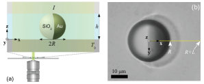
Figure 1: (a) Schematic representation of the side-view ($x$-$z$ plane) of the sample cell composed of two glass plates at separation $h\approx 2R$, where $R$ is the particle radius, which is suspended in a PnP-water mixture at its critical composition below $T_{c}$. At such confinement the particle is immobilized. Green laser illumination of intensity $I$ is applied onto the sample in the $z$-direction from above. (b) Sketch of the main particle axis along which the spatial variance of the order parameters is computed up to distance $L$ from the particle surface. The dark area on the right side of the colloid corresponds to the golden cap.

In the nonequilibrium steady state one observes a stable droplet covering the Janus particle asymmetrically; the droplet is much more pronounced near the hot golden cap (see Fig.1(b)). Our experimental data and results of numerical calculations within two theoretical models reveal that the reorganization of the concentration field around the Janus colloid until the steady state is reached is remarkably slow, whereas returning to the initial homogeneous distribution after switching off illumination is relatively fast. This asymmetry has not been noticed so far. The relaxation to a steady state and back to equilibrium in our system has curious features due to the presence of a temperature gradient. Among them is the power law of the early relaxation after switching on illumination (ON process). The power-law exponent $\approx 2$, as predicted from both purely diffusive and hydrodynamic models, is in excellent agreement with the experiment. This agreement supports the existence of a generic mechanism of the initial process connected to the formation of surface layers D0SM00964D . On the other hand, the relaxation to equilibrium after switching off the illumination (OFF process) is stretched exponential with a characteristic time decreasing as the illumination power increases, which we attribute to the temperature gradient previously formed by the laser-induced heating of the particle’s golden cap.

II Experimental results

In our experiments, we use a binary liquid mixture of propylene glycol n-propyl ether (PnP) and water, the lower critical point (LCP) of which is $T_{c}=31.9^{\circ}$C at its critical composition (0.4 PnP mass fraction) Bauduin2004 . In order to characterize the relaxation of such a binary liquid around the heated colloid, we study the time evolution of the image intensity profile $-\frac{1}{2}<\phi<\frac{1}{2}$ measured along the main particle axis, where $\phi$ is related to the concentration profile D0SM00964D . The value $\phi=0$ corresponds to the fully mixed fluid, whereas $\phi<0$ and $\phi>0$ represent locally water-rich and PnP-rich regions, respectively. Spatio-temporal variations of $\phi$ originate from the difference between the refractive index of water and PnP within the temperature range of the experiments ($30\pm 5^{\circ}$C), $n=1.331\pm 0.001$ and $n=1.410\pm 0.002$, respectively. In the mixed phase at $T_{0}<T_{c}$ and without laser illumination, the refractive index of the binary liquid in thermal equilibrium is homogeneous, thereby leading to a uniform light intensity pattern recorded by the camera around the Janus colloid. On the other hand, if the power of the incident laser is sufficiently high such that the golden cap reaches the temperature $T>T_{c}$, spatial variations of the refractive index due to the local phase separation of the fluid give rise to deviations of the light intensity recorded by the camera from the uniform intensity under thermal equilibrium conditions, which allows us to implement shadowgraph visualization ASSENHEIMER1994373 ; Mauger .

At a given time $t$, we compute the spatial variance of $\phi$ along $R<r<R+L$, defined as

$$\langle\Delta\phi(t)^{2}\rangle=\frac{1}{L}\int_{R}^{R+L}dr\,\left[\phi(r,t)-\langle\phi(t)\rangle\right]^{2},$$ (1)

where

$$\langle\phi(t)\rangle=\frac{1}{L}\int_{R}^{R+L}dr\,\phi(r,t),$$ (2)

is the spatial average of the order parameter $\phi(r,t)$ at time $t$ along the main particle axis, as shown in Fig.1(b). For all the calculations presented in the following, $L=25\,\mu$m, which is approximately two times the particle radius. Note that when the concentration profile has reached a steady state, $\langle\Delta\phi(t)^{2}\rangle$ remains constant over time, whereas a time dependence of $\langle\Delta\phi(t)^{2}\rangle$ reveals the transient behavior of the concentration field of the fluid during ON and OFF processes. On the other hand, the minimum value of $\langle\Delta\phi(t)^{2}\rangle$ is set by the intensity fluctuations on the colormap for a fully mixed binary liquid mixture, whose standard deviation is $\delta\phi_{0}\approx 0.03$.

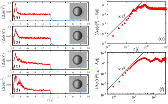
Figure 2: Time evolution of the spatial variance of the order parameter $\phi(r,t)$, computed along the main particle axis $R<r<R+L$ (with $L=25\,\mu$m), for different values of the temperature increase $\Delta T$ induced by optical heating. Panels (a), (b), (c) and (d) correspond to $\Delta T=7.8,9.1,10.4$ and $11.7^{\circ}$C, respectively. At time $t=-10$ s the laser illumination is switched on, thus leading the formation a nonequilibrium steady concentration field around the particle, while at $t=0$ it is switched off. Insets: images of the steady state at $t=-1$ s. Figures 2(e) and 2(f) show the initial growth of the spatial variance from the experiment ($\Delta T=7.8{{}^{\circ}}$C) and from the numerical simulations ($h=4$) of the hydrodynamic model, respectively. $\delta\phi_{0}^{2}=0.001$ and $\delta\varphi_{0}^{2}=0.00303$

Figure 2 shows the time evolution of $\langle\Delta\phi(t)^{2}\rangle$ for different values of the temperature increase $\Delta T=T-T_{0}=7.8,9.1,10.4,11.7^{\circ}$C of the golden cap of a Janus particle (radius $R=12\,\mu$m, strongly hydrophilic cap and weakly hydrophilic silica hemisphere) above the bath temperature $T_{0}=28^{\circ}\mathrm{C}<T_{c}$ and $T>T_{c}$ the temperature of the golden cap under green illumination. At time $t=-10$ s, the illumination is switched on, which leads to the transient coarsening process investigated in our previous paper D0SM00964D . Due to the heating of the particle, the concentration profile changes with respect to the initial uniform concentration in thermal equilibrium at temperature $T_{0}$, for which $\langle\phi(t)\rangle=0$ and $\langle\Delta\phi(t)^{2}\rangle=\delta\phi_{0}^{2}=0.001$. During the first $\sim 200$ ms, we observe a monotonic increase in the spatial variance, which can be described by a power law $\langle\Delta\phi(t)^{2}\rangle-\delta\phi_{0}^{2}\simeq t^{2}$ as shown in Fig.2(e). This initial growth can be attributed to the dynamics of the traveling composition layers D0SM00964D . Later the nonlinear growth of a water-rich droplet around the cap dominates, leading to a complex non-monotonic time dependence of $\langle\Delta\phi(t)^{2}\rangle$, with a maximum followed by a subsequent decay until it saturates to a mean constant value corresponding to the final nonequilibrium steady concentration field. It is worth noting that this behavior of the spatial variance of $\phi$ is similar to the initial overshoot in response to an external field found in diverse soft materials, such as actin networks levin2020kinetics , colloidal suspensions zia2013stress ; sentjabrskaja2014transient , polymer melts tseng2021constitutive , or a yield-stress fluids benzi2021stress . In our system, the maximum in $\langle\Delta\phi(t)^{2}\rangle$ results from local phase separation around the warmer part of the colloid after switching on illumination, which proceeds via a two-step process under a step-like temperature variation across the critical temperature- This mechanism shares some similarities with the origin of the overshoot in the nonlinear response of entangled polymer solutions ravindranath2008universal , where the stress overshoot is also a consequence of a two-step process under a step-like shear rate. In that case, there is an initial elastic energy storage mechanism (similar to the transient layering in our system) followed by a sudden dissipative energy release after the stress peak (in our system, the droplet formation). Significant fluctuations around the mean steady state value of $\langle\Delta\phi(t)^{2}\rangle$ occur due to the strong concentration fluctuations taking place inside the water-rich droplet, as will be discussed later. The duration of the transient state until the concentration field relaxes to the nonequilibrium steady state strongly depends on the value of the $\Delta T$. Interestingly, a further increase in $\Delta T$ gives rise to a qualitatively different behavior of the time evolution of $\langle\Delta\phi(t)^{2}\rangle$, in which the transient exhibits a very slow relaxation to the nonequilibrium steady state with strong concentration fluctuations and more than a single maximum - see Fig.2(c) and (d). This is correlated with the final shape of the water-rich droplet formed in the nonequilibrium steady state. In the case shown in Fig.2(a) and (b), the droplet covers partially the colloid surface (see the insets). However, for $\Delta T>9.1^{\circ}$C, the temperature is sufficiently high to form a droplet that completely surrounds the colloidal particle.

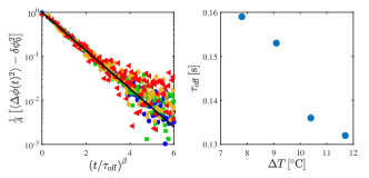
Figure 3: (a) Dependence on the rescaled time $(t/\tau_{\mathrm{off}})^{\beta}$ with $\beta=0.62$ of the difference between the spatial variance of $\phi(r,t)$ and the offset value $\delta\phi_{0}^{2}$, normalized by the amplitude $A$, after switching off the green illumination at time $t=0$ s, for different values of $\Delta T$ (symbols). The symbols correspond to: $\Delta T$ = 7.8^∘ C (blue circles), 9.1^∘ C (green squares), 10.4^∘ C (orange diamonds) and 11.7^∘ C (red triangles). The solid line represents Eq.(3). (b) Relaxation time $\tau_{\mathrm{off}}$ of nonequilibrium concentration profile after switching off the laser for different values of the temperature difference $\Delta T$.

The relaxation from the nonequilibrium steady concentration field under green illumination to a thermal-equilibrium state at temperature $T_{0}=28^{\circ}$C is achieved by switching off the laser at time $t=0$, as shown in Fig. 2. In this case, the time evolution of $\langle\Delta\phi(t)^{2}\rangle$ is monotonically decreasing in time for all values of $\Delta T$. In the long time limit, the spatial variance of the order parameter $\phi(r,t)$ reaches the constant value $\langle\Delta\phi(t)^{2}\rangle=\delta\phi_{0}^{2}=0.001$, thus revealing the full relaxation of the fluid to thermal equilibrium, where the concentration profile is uniform. As shown in Fig.3(a), the relaxation is well described by the stretched exponential

$$\langle\Delta\phi(t)^{2}\rangle=\delta\phi_{0}^{2}+A\exp\left[-\left(\frac{t}{\tau_{\mathrm{off}}}\right)^{\beta}\right],$$ (3)

with $\beta=0.62$ for all values of $\Delta T$, regardless of the shape of the nonequilibrium stationary droplet. As shown in Fig.3(b), the resulting values of the relaxation time $\tau_{\mathrm{off}}$ decrease upon increasing the temperature difference $\Delta T$. The stretch exponential, called in physics Kohlrausch–Williams–Watts (KWW) function wu2016heterogeneous ; lukichev2019physical , is known to describe relaxations if, e.g., each constituent particles relaxing exponentially through a single energy barrier, but there are different barrier heights for different particles such as in glassy systems xia2001microscopic ; welch2013dynamics , buckled colloidal monolayers han2008geometric , cytoskeletal networks lieleg2011slow , or the luminiscence decay of colloidal quantum dots bodunov2017origin . In our system, such a distribution of different barrier heights for the relaxation of the concentration field is produced by the spatial heterogeneity created by initial temperature gradient.

III Theoretical description

Our theoretical description of the relaxation process is based on the fluid particle dynamics method PhysRevLett.85.1338 . In this approach, the Janus particle is described by the shape function $\mathcal{S}(\mathbf{r},\mathbf{x})=\frac{1}{2}\left[1+\tanh\left(\frac{R-|\mathbf{r}-\mathbf{x}|}{d_{\mathcal{S}}}\right)\right],$ and the particle orientation function $\mathcal{O}(\mathbf{r},\mathbf{x},\mathbf{n})=\frac{1}{2}\left[1+\tanh\left(\frac{1}{d_{\mathcal{O}}}\mathbf{n}\cdot\frac{\mathbf{r}-\mathbf{x}}{|\mathbf{r}-\mathbf{x}|}\right)\right],$ where $\mathbf{r}$ is the coordinate of the lattice space and $\mathbf{x}$ is the position of the center of the particle. $d_{\mathcal{S}}$ represents the width of the smooth interface such that, in the limit of $d_{\mathcal{S}}\rightarrow 0$, $\mathcal{S}$ is unity and zero in the interior and exterior of the particle, respectively. $\mathbf{n}$ is the unit vector along the particle orientation, and $d_{\mathcal{O}}$ is a sharpness parameter of the particle orientation. Roughly, one has $\mathcal{O}=1$ on the capped side ($\mathbf{n}\cdot(\mathbf{r}-\mathbf{x})/|\mathbf{r}-\mathbf{x}|>d_{\mathcal{O}}$). Otherwise, one has $\mathcal{O}=0$. We consider a binary liquid mixture with an upper critical temperature of demixing (UCP), therefore heating by illumination in the experiment corresponds to cooling in our model. In our modeling, we focus on universal features of the system near the UCP, which are the same as for the LCP, in order to be able to compare with the experiment. If one would like to model the LCP beyond the universal features, one would have to take into account specific interactions, e.g., hydrogen bonding, that give rise to mixing in low temperatures. The mixture is characterized by the concentration field $\varphi(\mathbf{r})$, and the temperature field $T(\mathbf{r})$. The local energy density of the binary mixture $e(\varphi,\mathbf{x},\mathbf{n},T)$ is a sum of the kinetic energy $e_{T}(T)=\frac{3}{2}k_{\mathrm{B}}T$ and the interaction energy $e_{\varphi}(\varphi,\mathbf{x},\mathbf{n})=(1-\mathcal{S})\left[-\frac{\epsilon}{2}\varphi^{2}+\frac{C}{2}(\nabla\varphi)^{2}\right]+\frac{\chi_{\mathrm{p}}}{2}(\varphi-\varphi_{\mathrm{p}})^{2}\mathcal{S}+\left[W_{\mathrm{u}}+(W_{\mathrm{c}}-W_{\mathrm{u}})\mathcal{O}\right]\varphi|d_{\mathcal{S}}\nabla\mathcal{S}|$. $k_{\mathrm{B}}(=1)$ is the Boltzmann constant and $\epsilon(>0)$ is the interaction parameter. $W_{\mathrm{c}}$ and $W_{\mathrm{u}}$ represent the symmetry breaking surface fields. The second term in $e_{\varphi}$ is introduced to avoid solvent invasion into the particle. $\chi_{\mathrm{p}}$ and $\varphi_{\mathrm{p}}$ are its control parameters. Since $\varphi$ is conserved locally, its time development is given by the conservation law:

$$\frac{\partial\varphi}{\partial t} = -\nabla\cdot(\varphi\mathbf{v})-\nabla\cdot\left(-L_{\varphi}\frac{\mu}{T}\right)+\zeta(\mathbf{r},t),$$ (4)

$$\frac{\partial e}{\partial t} = -\nabla\cdot(e\mathbf{v})-\nabla\cdot\left(L_{T}\nabla\frac{1}{T}\right)-h\mathcal{O}|d_{\mathcal{S}}\nabla\mathcal{S}|,$$ (5)

where $L_{\varphi}$ and $L_{T}$ are positive kinetic coefficients. The Gaussian white noise $\zeta$ obeys the relation $\langle\zeta(\vec{r},t)\leavevmode\nobreak\ \zeta(\vec{r}^{\prime},t^{\prime})\rangle=-2\zeta_{0}\nabla^{2}\delta(\vec{r}-\vec{r}^{\prime})\delta(t-t^{\prime})$; $\zeta_{0}$ is the strength of the noise. We ignore the off-diagonal terms. $h$ represents the cooling power, and the temperature field is calculated from $e(\varphi,\mathbf{x},\mathbf{n},T)$. Because the system is nonisothermal, the chemical potential is calculated from the entropy density $s$ as $\mu=-T\left(\frac{\partial s}{\partial\varphi}\right)_{e}$. Expressions for $s$ and $\mu$ are given in Appendix A. In mean field, $\mu$ gives the critical point at $\varphi_{\mathrm{c}}=0$ and $T_{\mathrm{c}}=\epsilon/(ak_{\mathrm{B}})$. When $T<T_{\mathrm{c}}$, the UCP symmetric mixture is phase-separated. The velocity $\mathbf{v}(\mathbf{r})$ of the hydrodynamic flow obeys the following hydrodynamic equation:

$$C\nabla\cdot(\nabla\varphi:\nabla\varphi)-\frac{\mathcal{S}}{\Omega}\frac{\partial e}{\partial\mathrm{x}}-\frac{1}{2}\nabla\times\left\{\frac{\mathcal{S}}{\Omega}\mathbf{n}\times\left(\frac{\partial e}{\partial\mathbf{n}}\right)\right\}-\nabla p$$

$$+\nabla\left[\{\eta+(\eta_{\mathrm{c}}-\eta)\mathcal{S}\}\{\nabla:\mathbf{v}+(\nabla:\mathbf{v})^{T}\right]+\mathbf{F_{x}}=0.$$ (6)

The first term is the mechanical stress stemming from the concentration inhomogeneity, i.e., the interface tension. The second and third terms are due to the particle translation and rotation. $p$ is the pressure obtained by the incompressible condition $\nabla\cdot\mathbf{v}=0$. Within the FPD method, the fifth term is due to the viscous stress, in which $\eta$ and $\eta_{\mathrm{c}}$ are the viscosity of the solvent and the inside of the particle, respectively. The last term $\mathbf{F_{x}}=K(\mathbf{x}-\mathbf{x}_{0})\frac{\mathcal{S}}{\Omega}$ is introduced in order to fix the particle at its initial position $\mathbf{x}_{0}$ by imposing a harmonic potential with spring constant $K$. By neglecting the convection terms in Eqs.(4) and (5) the model reduces to the nonisothermal purely diffusive model of type B.

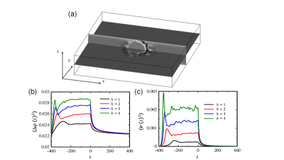
Figure 4: Numerical results of the hydrodynamic model: (a) Snapshot of the concentration field around the Janus particle at time $t=-400$. The capped surface (oriented toward the $x$ axis) is cooled with the power $h=4$; (b) Time evolution of the spatial variance $\langle\Delta\varphi(t)^{2}\rangle$ of the concentration field averaged over the whole sample for $h=4$; (c) Time evolution of the fluctuations $\langle v^{2}\rangle$ of the velocity field averaged over the whole sample for several values of the cooling power $h$.

IV Numerical results

We solve the evolution equations numerically (for details of numerical simulation see Appendix B). For the initial configuration we assume $\varphi(r,t)=0$ throughout, $T=1.1T_{\mathrm{c}}$ everywhere and no flow. At $t=-400$ we perform a temperature quench at the capped surface of the particle by switching on the cooling power $h$. At $t=0$ the cooling power is switched off and the time evolution is registered up to $t=400$. The snapshot of the concentration field $\varphi(r,t)$ at $t=0$ and $h=4$ is shown in Fig.4(a). The binary solvent is phase separated around the colloid forming an asymmetric droplet within which the concentration field strongly fluctuates. Fig.4(b) shows how the spatial variance $\langle\Delta\varphi(t)^{2}\rangle$ of the concentration field averaged over the whole sample changes in the whole period of time for various temperature quenches. Velocity fluctuations are shown in Fig.$\ref{Fig:Hprofiles}(c)$.

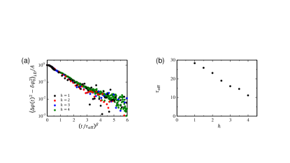
Figure 5: Numerical results of the hydrodynamic model: (a) Fitting numerical results for normalized spatial variance $\langle\Delta\varphi(r,t)(t)^{2}\rangle_{1D}$ of the concentration field calculated along the main particle axis during the OFF process to the stretched exponential decay given by Eq.(3) (dashed line) with $\beta=0.62$, for different values of $h$ (symbols). $\delta\varphi_{0}=0.00303$. (b) Relaxation time $\tau_{\mathrm{off}}$ of nonequilibrium concentration profile after switching off cooling for different values of the cooling power $h$.

During the ON process $\langle\Delta\varphi(t)^{2}\rangle$ resulting from the hydrodynamic model exhibits a noisy nonmonotonic behavior which is very similar to the behavior of $\langle\Delta\phi(t)^{2}\rangle$ observed in experiment. On the contrary, purely diffusive model B gives a smooth and monotonic evolution towards the steady state (see Fig.7(a) in Appendix C). It is well established that thermal fluctuations in liquids in the presence of stationary temperature gradients are anomalously large and very long-ranged de2006hydrodynamic . They occur as a result of a coupling between temperature and velocity fluctuations. In liquid mixtures a stationary temperature gradient induces stationary concentration gradient via the Soret effect. Fluctuating hydrodynamics for a binary fluid mixtures bounded between two parallel plates with different temperatures predicts that nonequilibrium fluctuations of concentration, temperature, as well as velocity will be present at a stationary state of a mixture croccolo2016non . However, because in liquid mixtures the ratio between thermal diffusivity and the mass diffusion coefficient (Lewis number) and the ratio between the kinematic viscosity and the mass diffusion coefficient (Schmidt number) are commonly larger than unity, nonequilibrium fluctuations in concentration will be dominant. Here we study nonequilibrium fluctuations not only at a stationary state, but also when approaching it. In the initial stage, the hydrodynamic flow is weak so that both hydrodynamic and purely diffusive models give a similar growth of concentration fluctuations: $\langle\Delta\varphi(r,t)(t)^{2}\rangle_{1D}$ calculated along the main particle axis $R<r<R+L$ with $L=100$ in the $x$–$y$ plane passing through the particle can be described by the power law $\sim t^{2}$ (see Figs.2(f) and 7(b) in Appendix C), in a perfect agreement with the experimental data. We stress that this initial behavior cannot be described by linearized equations. In the late stage, on the other hand, the concentration fluctuations are caused by coupling between the concentration and velocity fields, because the Lewis number is large in our simulations. From Figs.4(b) and (c), we can see that for our choice of parameters the velocity fluctuations are comparable with the concentration fluctuations. Other predictions of fluctuating hydrodynamics indicate that the intensity of nonequilibrium fluctuations is proportional to $\left(\nabla T\right)$ and that for small wave numbers $q$ the intensity of the nonequilibrium concentration fluctuations diverges as $q^{-4}$, which is much stronger than the divergence of critical concentration fluctuations as $q^{-2}$ near a consolute point croccolo2016non . Comparing our experimental data shown in Figs.2(a) and (d) and the theoretical curves for $h=1$ and $h=4$ in Figs.4(b) and (c) we can conjecture that indeed, thermal fluctuations are stronger for larger temperature gradients. Due to technical difficulties, we have not analyzed the $q$-dependence of our results.

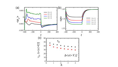
Figure 6: Evolution of (a) the concentration field contribution $\langle e_{\varphi}\rangle$ to the energy and of (b) the total energy $\langle e\rangle$ of the system for different values of the cooling power $h$. $\langle e\rangle$ and $\langle e_{\varphi}\rangle$ are the spatial averages of $e$ and $e_{\varphi}$.(c) Initial decay time $\tau_{0}$ of the total energy $\langle e\rangle$ after switching off the laser and the ratio $\Delta\langle e(t=0)\rangle V/J$ between the energy stored in the steady state and the total energy flux at this state for different values of $h$. $V$ is the system volume.

In the simulations, we also observe that returning to equilibrium is much faster than approaching the steady state. Remarkably, during the OFF process the time dependence of $\langle\varphi(r,t)(t)^{2}\rangle_{1D}$ is well described by Eq.(3) with the same exponent $\beta=0.62$ as in the experiment, as shown in Fig.5. The characteristic time of the stretched exponential decay decreases with the cooling power. This trend is also similar to the one observed in the experiment. With increasing values of $h$ or $\Delta T$, a larger temperature gradient builds up around the colloid, which speeds up relaxation to the equilibrium. Next, we compute the energy of the system, which is practically not accessible from experiment. As can be inferred from Fig.6(a) and (b), $\langle e\rangle$ is dominated by the kinetic contribution $\langle e_{T}\rangle$ and hence it decreases after the cooling is switched on and increases upon switching off the cooling power. Restructuring of the concentration field in response to the temperature changes is much slower in both ON and OFF processes, as mirrored in the evolution of $\langle e_{\varphi}\rangle$. Achieving the nonequilibrium stationary value of $\langle e_{\varphi}\rangle$ takes longer because the initial concentration field is uniformly distributed whereas returning to equilibrium starts from a concentrated distribution and therefore is faster (see movies in SM). Finally, relaxation of the energy to equilibrium is well described by Eq.(3) with the exponent $\beta=0.62$ and the characteristic decay time $\tau_{\textrm{off}}$ which decreases with $h$ as can be seen in Fig.6(c). Decay of $\langle\varphi(r,t)(t)^{2}\rangle_{1D}$ and $\langle e_{T}\rangle$ in the purely diffusive model B is better described by a sum of the exponential end stretched exponential functions of time - see Appendix C. We find that $\tau_{\textrm{off}}$ is almost the same as the initial decay time $\tau_{0}$ obtained from the change rate of the energy at $t=0$. Interestingly, both characteristic times are proportional to the ratio $\mathcal{T}$ between the energy stored in the nonequilibrium steady state and the total energy flux in this state $\mathcal{T}=\Delta\langle e(t=0)\rangle V/J$- see Fig.6(c). The same holds for the initial decay time $\tau_{0}$ obtained in model B, as can be seen in Fig.8(d) in Appendix C. Similar observation was made for the energy out-flow from the Lennard-Jones system - but only for initial times after the shutdown of energy flux into the system PhysRevE.99.042118 .

V Summary

In summary, we have investigated the relaxation process of the concentration field of a binary mixture around a Janus colloid heated by laser illumination through the critical temperature of the fluid. Our results show a pronounced asymmetry in the approach to a nonequilibrium state under a temperature gradient around the colloid with respect to the relaxation of the fluid back to equilibrium at constant temperature. While in the former the dynamics is dominated by transient composition layers until the final noisy steady state is reached, the latter is faster and follows a stretched-exponential decay consistent with the characteristic timescale of energy outflow after the shutdown of the energy input. In particular, we show that such relaxation timescale is directly related to the energy stored in the nonequilibrium steady state and the total energy flux. Further experimental and theoretical efforts could help to address the connection between these two quantities with the relaxation from nonequilibrium states in other systems.

VI Acknowledgments

A. M. thanks Sutapa Roy for discussions on the purely diffusive model. T.A. is financially supported by KAKENHI (Grant No.21K03486), and CREST, JST (JPMJCR2095). J. R. G.-S. was supported by UNAM-PAPIIT IA103320

Appendix A Entropy density and chemical potential of the hydrodynamic model

Close to the critical point the entropy density can be written as

$$s(\varphi,\mathbf{x},T)=-k_{\mathrm{B}}(1-\mathcal{S})\left(\frac{a}{2}\varphi^{2}+\frac{b}{4}\varphi^{4}\right)+k_{\mathrm{B}}\left[\ln\left(\frac{v}{\lambda_{T}^{3}}\right)+1\right],$$ (7)

where $a$ and $b$ are positive constants, $\lambda_{T}(\propto T^{-1/2}$) is the thermal de Broglie length, and $v$ is the molecular volume, thus

$$\mu = (1-\mathcal{S})\left[(k_{\mathrm{B}}Ta-\epsilon)\varphi+k_{\mathrm{B}}Tb\varphi^{3}\right]-C\nabla\cdot\left[(1-\mathcal{S})\nabla\varphi\right]$$ (8)

$$+[W_{\mathrm{u}}+(W_{\mathrm{c}}-W_{\mathrm{u}})\mathcal{O}]|d_{\mathcal{S}}\nabla\mathcal{S}|+\chi_{\mathrm{p}}(\varphi-\varphi_{\mathrm{p}})\mathcal{S}.$$

Appendix B Parameters of the numerical simulations

The simulation box has size $240\times 240\times 52$ in units of the lattice spacing $\Delta=1$. The walls are placed at $z=1$ and $z=52$. The non-slip boundary conditions for the hydrodynamic flow are imposed at the walls, i.e., $\mathbf{v}(z=1)=\mathbf{v}(z=52)=0$. The temperatures at the walls are kept above the critical temperature $T(z=1)=T(z=52)=1.1T_{\mathrm{c}}$. The concentration flux $-L_{\varphi}\nabla(\mu/T)$ is imposed to vanish at the walls. The periodic boundary conditions are applied to the $x$ and $y$ directions. The time increment is $\Delta t=0.001$. We take the particle radius $R=20$ and set $d_{\mathcal{S}}=1$ and $d_{\mathcal{O}}=0.033$. The capped surface is strongly hydrophilic with $W_{\mathrm{c}}=-2.0$, while the uncapped surface is weakly hydrophilic with $W_{\mathrm{u}}=-0.2$. In Eq. (8) we set $\epsilon=1$, $C=4$, $\chi_{\mathrm{p}}=5$, $\varphi_{\mathrm{p}}=0$, $a=1$ and $b=1$. In equations for time evolution (Eqs. (4) and (5)), we employ $L_{\varphi}=(1-\mathcal{S})$, $L_{T}=10(1+2\mathcal{S})$, and $\zeta_{0}=10^{-4}$. In the hydrodynamic equation (6), we set $\eta=0.5$, $\eta_{\mathrm{c}}=25$ and $K=100$.

Calculation of stationary state fluxes The inlet and outlet fluxes are calculated as

$$J_{\mathrm{in}} = \int\mathrm{d}\mathbf{r}h\mathcal{O}|d_{\mathcal{S}}\nabla\mathcal{S}|,$$ (9)

$$J_{\mathrm{out}} = \int\mathrm{d}\mathbf{A}\cdot L_{T}\nabla\frac{1}{T},$$ (10)

where $\int\mathrm{d}\mathbf{A}$ represents the integral over the two walls.

Appendix C Results from the purely diffusive model B

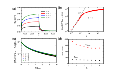
Figure 7: Numerical results from the purely diffusive model B. (a) Time evolution for the spatial variance $\langle\Delta\varphi(t)^{2}\rangle$ of the concentration field averaged over the whole system for different values of the cooling power $h$; (b) The initial growth of $\langle\Delta\varphi(t)^{2}\rangle_{1D}$ of the concentration field calculated along the main particle axis after switching on cooling at $t=-5000$. $\delta\varphi_{0}^{2}=0.00303$; (c) Normalized $\langle\Delta\varphi(t)^{2}\rangle_{1D}$ after switching off cooling at time $t=0$ for different values of $h$. The horizontal axis is scaled with the characteristic decay time of the fast mode (see Eq. (11)). (d) The $h$ dependence of two times $\tau_{\textrm{fast}}$ and $\tau_{\textrm{slow}}$ characterizing the decay of $\langle\Delta\varphi(t)^{2}\rangle_{1D}$ after switching off cooling obtained from fitting to the function $f(t)$ given by Eq. (11) with $\beta\approx 0.62$.

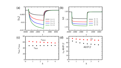
Figure 8: Numerical results for time evolution of (a) the contribution $\langle e_{\varphi}\rangle$ to the total energy density due to the concentration field and of (b) the total energy density $\langle e\rangle$ of the system calculated within the purely diffusive model B for different values of the cooling power $h$. $\langle e\rangle$ and $\langle e_{\varphi}\rangle$ are the spatial averages of $e$ and $e_{\varphi}$, where $V$ is the system volume. (c) The $h$ dependence of two times $\tau_{\textrm{fast}}$ and $\tau_{\textrm{slow}}$ characterizing the decay of $\langle e\rangle$ after switching off cooling obtained from fitting to the function $f(t)$ given by Eq. (11). (d) Initial decay time $\tau_{0}$ of $\langle e\rangle$ after switching off the laser and the ratio $\Delta\langle e(t=0)\rangle V/J$ between the energy stored in the steady state and the total energy flux at this state for different values of $h$.

The cooling power is applied at $t=-5000$ and removed at $t=0$. The spatial variance $\langle\Delta\varphi(t)^{2}\rangle$ of the concentration field averaged over the whole system increases monotonically until the cooling is switched off (Fig. 7(a)). After a rapid initial growth, which is due to concentration waves traveling from the surface, $\langle\Delta\varphi(t)^{2}\rangle$ approaches the steady state value logarithmically. The initial growth of the concentration field $\langle\Delta\varphi(t)^{2}\rangle_{1D}$ calculated along the main particle axis follows well the power law $\approx t^{2}$, in agreement with experimental and hydrodynamic model results (Fig. 7(b)).

The decay of $\langle\Delta\varphi(t)^{2}\rangle_{1D}$ after the removal of $h$ is fitted well by the function

$$f(t)=a_{1}\exp(-t/\tau_{\textrm{fast}})+a_{2}\exp(-(t/\tau_{\textrm{slow}})^{\beta})+c$$ (11)

with experimental value $\beta\approx 0.62$. Characteristic time $\tau_{\textrm{fast}}$ of fast exponential decay dominating at very short times is almost independent of the cooling power. Time $\tau_{\textrm{slow}}$ characterizing the stretched exponential decay decreases with increasing cooling power. If we treat $\beta$ in Eq. (11) as a fitting parameter, both characteristic times change only slightly. The fitted values of $\beta$ varies from $\approx 0.72$ for $h=0.5$ to $\approx 0.62$ for $h=4$.

Results for the total energy density $\langle e\rangle$ averaged over the system and the contribution to it from the concentration field $\langle e_{\varphi}\rangle$ are shown in Fig. 8. After switching off cooling $e$ is also well described by Eq. (11) with the stretched exponent $\beta\approx$ 0.58.

References

- (1) L. Onsager, “Reciprocal relations in irreversible processes. i.”, Phys. Rev. 37, 405 (1931).
- (2) L. Onsager, “Reciprocal relations in irreversible processes. ii.”, Phys. Rev. 38, 2265 (1931).
- (3) R. Kubo, M. Yokota, and S. Nakajima, “Statistical-mechanical theory of irreversible processes. ii. response to thermal disturbance”, J. Phys. Soc 12, 1203 (1957).
- (4) S. Dattagupta, Relaxation phenomena in condensed matter physics, Elsevier (2012).
- (5) R. Metzler, E. Barkai, and J. Klafter, “Anomalous diffusion and relaxation close to thermal equilibrium: A fractional fokker-planck equation approach”, Phys. Rev. Lett. 82, 3563 (1999).
- (6) N. Shiraishi and K. Saito, “Information-theoretical bound of the irreversibility in thermal relaxation processes”, Phys. Rev. Lett. 123, 110603 (2019).
- (7) A. Lapolla and A. Godec, “Faster uphill relaxation in thermodynamically equidistant temperature quenches”, Phys. Rev. Lett. 125, 110602 (2020).
- (8) C. Maes, K. Netočný, and B. Wynants, “Monotonic return to steady nonequilibrium”, Phys. Rev. Lett. 107, 010601 (2011).
- (9) L. V. F. Gomes and A. B. Kolomeisky, “Dynamics of relaxation to a stationary state for interacting molecular motors”, J. Phys. A 51, 015601 (2017).
- (10) A. Dhar, A. Kundu, S. N. Majumdar, S. Sabhapandit, and G. Schehr, “Run-and-tumble particle in one-dimensional confining potentials: Steady-state, relaxation, and first-passage properties”, Phys. Rev. E 99, 032132 (2019).
- (11) J. R. Gomez-Solano, A. Petrosyan, S. Ciliberto, R. Chetrite, and K. Gawędzki, “Experimental verification of a modified fluctuation-dissipation relation for a micron-sized particle in a nonequilibrium steady state”, Phys. Rev. Lett. 103, 040601 (2009).
- (12) V. Blickle, J. Mehl, and C. Bechinger, “Relaxation of a colloidal particle into a nonequilibrium steady state”, Phys. Rev. E 79, 060104 (2009).
- (13) J. Gieseler, L. Novotny, C. Moritz, and C. Dellago, “Non-equilibrium steady state of a driven levitated particle with feedback cooling”, New J. Phys. 17, 045011 (2015).
- (14) J. A. Owen, T. R. Gingrich, and J. M. Horowitz, “Universal thermodynamic bounds on nonequilibrium response with biochemical applications”, Phys. Rev. X 10, 011066 (2020).
- (15) U. Basu, L. Helden, and M. Krüger, “Extrapolation to nonequilibrium from coarse-grained response theory”, Phys. Rev. Lett. 120, 180604 (2018).
- (16) G. Baffou and R. Quidant, “Thermo-plasmonics: using metallic nanostructures as nano-sources of heat”, Laser Photon. Rev. 7, 171 (2013).
- (17) A. Torchi, F. Simonelli, R. Ferrando, and G. Rossi, “Enhancement of lipid membrane permeability induced by irradiated gold nanoparticles”, ACS Nano 11, 12553 (2017).
- (18) A. Bahadori, G. Moreno-Pescador, L. B. Oddershede, and P. M. Bendix, “Remotely controlled fusion of selected vesicles and living cells: a key issue review”, Rep. Prog. Phys. 81, 032602 (2018).
- (19) G. Volpe, I. Buttinoni, D. Vogt, H.-J. Kümmerer, and C. Bechinger, “Microswimmers in patterned environments”, Soft Matter 7, 8810 (2011).
- (20) I. Buttinoni, G. Volpe, F. Kümmel, G. Volpe, and C. Bechinger, “Active brownian motion tunable by light”, J. Phys.: Condens. Matter 24, 284129 (2012).
- (21) J. R. Gomez-Solano, A. Blokhuis, and C. Bechinger, “Dynamics of self-propelled janus particles in viscoelastic fluids”, Phys. Rev. Lett. 116, 138301 (2016).
- (22) S. Kumar, A. Kumar, M. Gunaseelan, R. Vaippully, D. Chakraborty, J. Senthilselvan, and B. Roy, “Trapped in out-of-equilibrium stationary state: Hot brownian motion in optically trapped upconverting nanoparticles”, Front. Phys. 8, 429 (2020).
- (23) H. R. Vutukuri, M. Lisicki, E. Lauga, and J. Vermant, “Light-switchable propulsion of active particles with reversible interactions”, Nat. Commun. 11, 1 (2020).
- (24) S. Auschra, A. Bregulla, K. Kroy, and F. Cichos, “Thermotaxis of janus particles”, Eur. Phys. J. E 44, 90 (2021).
- (25) A. Girot, N. Danné, A. Würger, T. Bickel, F. Ren, J. Loudet, and B. Pouligny, “Motion of optically heated spheres at the water–air interface”, Langmuir 32, 2687 (2016).
- (26) F. Schmidt, A. Magazzù, A. Callegari, L. Biancofiore, F. Cichos, and G. Volpe, “Microscopic engine powered by critical demixing”, Phys. Rev. Lett. 120, 068004 (2018).
- (27) F. Schmidt, H. Šípová-Jungová, M. Käll, A. Würger, and G. Volpe, “Non-equilibrium properties of an active nanoparticle in a harmonic potential”, Nat. Commun. 12, 1 (2021).
- (28) A. Onuki, Phase transition dynamics, Cambridge University Press (2002).
- (29) M. Shono, S. Takatori, J. M. Carnerero, and K. Yoshikawa, “Switching between positive and negative movement near an air/water interface through lateral laser illumination”, Appl. Phys. Lett. 117, 073701 (2020).
- (30) M. Pascual, A. Poquet, A. Vilquin, and M.-C. Jullien, “Phase separation of an ionic liquid mixture assisted by a temperature gradient”, Phys. Rev. Fluids 6, 024001 (2021).
- (31) T. Zinn, L. Sharpnack, and T. Narayanan, “Phoretic dynamics of colloids in a phase separating critical liquid mixture”, Phys. Rev. Research 2, 033177 (2020).
- (32) C. Bechinger, R. Di Leonardo, H. Löwen, C. Reichhardt, G. Volpe, and G. Volpe, “Active particles in complex and crowded environments”, Rev. Mod. Phys. 88, 045006 (2016).
- (33) S. Roy, S. Dietrich, and A. Maciołek, “Solvent coarsening around colloids driven by temperature gradients”, Phys. Rev. E 97, 042603 (2018).
- (34) S. Roy and A. Maciołek, “Phase separation around a heated colloid in bulk and under confinement”, Soft Matter 14, 9326 (2018).
- (35) A. Würger, “Self-diffusiophoresis of janus particles in near-critical mixtures”, Phys. Rev. Lett. 115, 188304 (2015).
- (36) J. R. Gomez-Solano, S. Samin, C. Lozano, P. Ruedas-Batuecas, R. van Roij, and C. Bechinger, “Tuning the motility and directionality of self-propelled colloids”, Sci. Rep. 7, 1 (2017).
- (37) T. Araki and A. Maciołek, “Illumination-induced motion of a janus nanoparticle in binary solvents”, Soft Matter 15, 5243 (2019).
- (38) J. R. Gomez-Solano, S. Roy, T. Araki, S. Dietrich, and A. Maciołek, “Transient coarsening and the motility of optically heated janus colloids in a binary liquid mixture”, Soft Matter 16, 8359 (2020).
- (39) P. Bauduin, L. Wattebled, S. Schrödle, D. Touraud, and W. Kunz, “Temperature dependence of industrial propylene glycol alkyl ether/water mixtures”, J. Mol. Liq. 115, 23 (2004).
- (40) M. Assenheimer, B. Khaykovich, and V. Steinberg, “Phase separation of a critical binary mixture subjected to a temperature gradient”, Phys. A: Stat. Mech. Appl. 208, 373 (1994).
- (41) C. Mauger, L. Méès, M. Michard, A. Azouzi, and S. Valette, “Shadowgraph, schlieren and interferometry in a 2d cavitating channel flow”, Exp. in Fluids 53, 1895 (2012).
- (42) M. Levin, R. Sorkin, D. Pine, R. Granek, A. Bernheim-Groswasser, and Y. Roichman, “Kinetics of actin networks formation measured by time resolved particle-tracking microrheology”, Soft Matter 16, 7869 (2020).
- (43) R. N. Zia and J. F. Brady, “Stress development, relaxation, and memory in colloidal dispersions: Transient nonlinear microrheology”, J. Rheol. 57, 457 (2013).
- (44) T. Sentjabrskaja, M. Hermes, W. Poon, C. Estrada, R. Castaneda-Priego, S. Egelhaaf, and M. Laurati, “Transient dynamics during stress overshoots in binary colloidal glasses”, Soft Matter 10, 6546 (2014).
- (45) H.-C. Tseng, “A constitutive analysis of stress overshoot for polymer melts under startup shear flow”, Phys. Fluids 33, 051706 (2021).
- (46) R. Benzi, T. Divoux, C. Barentin, S. Manneville, M. Sbragaglia, and F. Toschi, “Stress overshoots in simple yield stress fluids”, Phys. Rev. Lett. 127, 148003 (2021).
- (47) S. Ravindranath and S.-Q. Wang, “Universal scaling characteristics of stress overshoot in startup shear of entangled polymer solutions”, J. Rheol. 52, 681 (2008).
- (48) J. H. Wu and Q. Jia, “The heterogeneous energy landscape expression of kww relaxation”, Sci. Rep 6, 1 (2016).
- (49) A. Lukichev, “Physical meaning of the stretched exponential kohlrausch function”, Phys. Lett. A 383, 2983 (2019).
- (50) X. Xia and P. G. Wolynes, “Microscopic theory of heterogeneity and nonexponential relaxations in supercooled liquids”, Phys. Rev. Lett. 86, 5526 (2001).
- (51) R. C. Welch, J. R. Smith, M. Potuzak, X. Guo, B. F. Bowden, T. Kiczenski, D. C. Allan, E. A. King, A. J. Ellison, and J. C. Mauro, “Dynamics of glass relaxation at room temperature”, Phys. Rev. Lett. 110, 265901 (2013).
- (52) Y. Han, Y. Shokef, A. M. Alsayed, P. Yunker, T. C. Lubensky, and A. G. Yodh, “Geometric frustration in buckled colloidal monolayers”, Nature 456, 898 (2008).
- (53) O. Lieleg, J. Kayser, G. Brambilla, L. Cipelletti, and A. R. Bausch, “Slow dynamics and internal stress relaxation in bundled cytoskeletal networks”, Nat. Mater. 10, 236 (2011).
- (54) E. Bodunov, Y. A. Antonov, and A. L. Simões Gamboa, “On the origin of stretched exponential (kohlrausch) relaxation kinetics in the room temperature luminescence decay of colloidal quantum dots”, J. Chem. Phys. 146, 114102 (2017).
- (55) H. Tanaka and T. Araki, “Simulation method of colloidal suspensions with hydrodynamic interactions: Fluid particle dynamics”, Phys. Rev. Lett. 85, 1338 (2000).
- (56) J. M. O. De Zárate and J. V. Sengers, Hydrodynamic fluctuations in fluids and fluid mixtures, Elsevier (2006).
- (57) F. Croccolo, J. O. de Zárate, and J. Sengers, “Non-local fluctuation phenomena in liquids”, Eur. Phys. J. E 39, 1 (2016).
- (58) R. Holyst, A. Maciołek, Y. Zhang, M. Litniewski, P. Knychała, M. Kasprzak, and M. Banaszak, “Flux and storage of energy in nonequilibrium stationary states”, Phys. Rev. E 99, 042118 (2019).