Efficient Quantum Feature Extraction for CNN-based Learning

Abstract

Recent work has begun to explore the potential of parametrized quantum circuits (PQCs) as general function approximators. In this work, we propose a quantum-classical deep network structure to enhance classical CNN model discriminability. The convolutional layer uses linear filters to scan the input data. Moreover, we build PQC, which is a more potent function approximator, with more complex structures to capture the features within the receptive field. The feature maps are obtained by sliding the PQCs over the input in a similar way as CNN. We also give a training algorithm for the proposed model. The hybrid models used in our design are validated by numerical simulation. We demonstrate the reasonable classification performances on MNIST and we compare the performances with models in different settings. The results disclose that the model with ansatz in high expressibility achieves lower cost and higher accuracy.

I Introduction

Quantum Computers use the principles of quantum mechanics for computing, which are considered more powerful than classical computers in some computing problems. In view of the rapid progresses in quantum computing hardware arute2019quantum , we are entering into so called NISQ era preskill2018quantum . Noisy intermediate scale quantum (NISQ) devices will be the only quantum devices that can be reached in near-term, where we can only use a limited number of qubits with little error correction. Thus, developing a useful computational algorithm using the NISQ devices is the urgent task at present.

Quantum machine learning (QML) biamonte2017quantum is gaining attention in the hope of speeding up machine learning tasks with quantum computers. Combing quantum computing and machine learning, QML attempts to utilize the power of quantum computers to achieve computational speedups or better performance for some machine learning tasks. Many quantum machine learning algorithms, such as qSVM rebentrost2014quantum , qPCA lloyd2014quantum and quantum Boltzmann machine amin2018quantum , have been developed. Recently, several NISQ algorithms, such as quantum transfer learning mari2020transfer and quantum kernel methods havlivcek2019supervised ; schuld2019quantum , have been proposed. On the other hand, parameterized quantum circuits benedetti2019parameterized provide an another path for QML toward quantum advantages in NISQ era. Compared to conventional quantum algorithms, such as Shor’s algorithm shor1999polynomial , Grover’s algorithm grover1997quantum , HHL algorithm harrow2009quantum , PQC based quantum-classical hybrid algorithms are inherently robust to noise and could benefit from quantum advantages, by taking advantage of both the high dimensional Hilbert space of a quantum system and the classical optimization scheme. Several popular related algorithms have been proposed, including variational quantum eigensolvers (VQE) peruzzo2014variational ; wecker2015progress ; mcclean2016theory and quantum approximate optimization algorithm (QAOA) farhi2014quantum ; hadfield2019quantum .

In addition, quantum neural networks (QNNs) schuld2014quest ; farhi2018classification ; lloyd2020quantum based on parameterized quantum circuits have been proposed. Some of QNN models utilized the thoughts of Convolutional Neural Network (CNN), which is a popular machine learning model on the classical computer. Cong et al. cong2019quantum designed a quantum circuit model with a similar hierarchy to classical CNNs, which dealt with quantum data and could be used to recognize phases of quantum states and to devise a quantum error correction scheme. The convolutional and pooling layers were approximated by quantum gates with adjustable parameters. Ref. henderson2020quanvolutional proposed a new quanvolutional (short for quantum convolutional) filter, in which a random quantum circuit was deployed to transform input data locally. Quanvolutional filters were embedded into classical CNNs, forming a quantum-classical hybrid structure. In addition, a more complex QCNN design was presented in recent works Kerenidis2020Quantum ; li2020quantum ; zheng2021speeding , where delicate quantum circuits were employed to accomplish quantum inner product computations and approximate nonlinear mappings of activation functions.

In this work, we propose a type of hybrid quantum-classical neural network based on PQCs for in analogy with the CNN. As a popular scheme in machine learning field, CNN replaces the fully connected layer with a convolutional layer. The convolutional layer only connects each neuron of the output to a small region of the input which is referred to as a feature map, thus greatly reducing the number of parameters. However, the filter in classical CNN model is a generalized linear model (GLM). It is difficult for linear filters to extract the concepts are generally highly nonlinear function of the data patch. In Network-in-Network (NiN) lin2013network , the linear filter replaced with a multilayer perceptron which is a general function approximator. As a “micro network”, multilayer perceptron can improve the abstraction ability of the model. In the field of QML, PQCs are considered as the “quantum network” structures. Recent works schuld2021effect ; goto2021universal ; liu2021hybrid shown that there exist PQCs which are universal function approximators with a proper data encoding strategy. Combining these ideas, we replace the linear filter with a PQC. The resulting structure is called the quantum feature extraction layer.

The key idea of our hybrid neural network is to implement the feature map in the convolutional layer with quantum parameterized circuits, and correspondingly, the output of this feature map is a correlational measurement on the output quantum state of the parameterized circuits. Different from Ref. henderson2020quanvolutional , which uses parameters fixed circuits, we can iteratively update the parameters of circuits to get better performance. We also give the training algorithm of this hybrid quantum-classical neural network which are similar to backpropagation (BP) algorithm, meaning that our model is trained as a whole. Hence it can be trained efficiently with NISQ devices. Therefore, our scheme could utilize all the features of classical CNN, and is able to utilize the power of current NISQ processors. Notice that the methods of data encoding and decoding are different from henderson2020quanvolutional .

This paper is organized as follows. Section II is the preliminary, in which we first review the classical convolution neural network and the framework of PQCs. Then, the proposed quantum-classical hybrid model is described in detail in Section III. In Section IV, we present numerical simulation where we apply the hybrid model to image recognition and analyze the result. Conclusion and discussion are given in Section V.

II Preliminaries

II.1 Supervised learning: construct a classifier

In a supervised classification task, we are given a training set $T$ and a test set $S$ on a label set $C$. Assuming there exists a map $m:T\cup S\rightarrow C$ unknown to the algorithm. Our task is to construct a model to infer an approximate map on the test set $\tilde{m}:S\rightarrow C$ only receiving the labels of the training set such that the difference between $m(s)$ and $\tilde{m}(s)$ is small on the test set $s\in S$. For such a learning task to be meaningful it is assumed that there is a correlation between the labels given for training set and the true map. A popular approach to this problem is to use neural networks(NNs), where the training data goes through the linear layer and the activation function repeatedly to map the true label. After constructing a NNs model that is accurate enough, we can perform the prediction of test set.

II.2 Convolution neural network(CNN)

CNN dates back decades lecun1989backpropagation ; lecun1998gradient which is a specialized kind of neural network for processing data that has a known grid-like topology. Deep CNNs have recently shown an explosive popularity partially due to its success in image classification krizhevsky2012imagenet . It also has been successfully applied to other fields, such as objection detection redmon2016you , semantic segmentation long2015fully and pedestrian detection zhang2016faster , even for natural language processing(NLP) vaswani2017attention .

Though there are several architectures of CNN models such as LeNet lecun1998gradient , AlexNet krizhevsky2012imagenet , GoogLeNet szegedy2015going , VGG simonyan2014very , ResNet he2016deep and DenseNet huang2017densely , they use three main types of layers to build CNN models: convolutional layer, pooling layer and fully-connected layer. Broadly, a CNN model can be divided into two parts: feature extraction module and classifier module. The former includes convolutional layer and pooling layer while the classifier module consists of fully-connected layers.

Formally, a convolutional layer is expressed as an operation $f_{1}$:

$$f_{1}(\textbf{X})=g(\textbf{W}_{1}*\textbf{X}+\textbf{B}_{1}),$$ (1)

where $\textbf{W}_{1}$ and $\textbf{B}_{1}$ represent the filters weights and biases respectively, and ‘$*$’ denotes the convolution operation. Concretely, $\textbf{W}_{1}$ corresponds to $n_{c}$ filters of support $f\times f\times c$, where $c$ is the number of channels in the input X, $f$ is the spatial size of a filter. Intuitively, $\textbf{W}_{1}$ applies $n_{c}$ convolutions on the input, and each convolution has a kernel size $f\times f\times c$. The output is composed of $n_{c}$ feature maps. $\textbf{B}_{1}$ is a $n_{c}$-dimensional vector, whose each element is associated with a filter. $g(\cdot)$ is an activation function which element-wisely apply a nonlinear transformation ,such as ReLU or Tanh, on the filter responses.

A pooling layer is generally added after the convolutional layer. Its function is to progressively reduce the spatial size of the representation to reduce the amount of parameters and computation in the network. Two commonly used pooling operations are max pooling and average pooling. The former calculates the maximum value for each patch of the feature map while the latter calculates the average value for each patch on the feature map. And the units in a fully-connected layer have full connections to all activations in the previous layer, as seen in regular neural networks.The activations are computed with a matrix multiplication followed by a bias offset, as shown in the operation $f_{2}$:

$$f_{2}(\textbf{x})=h(\textbf{W}_{2}\textbf{x}+\textbf{B}_{2}),$$ (2)

where x, $\textbf{W}_{2}$, $\textbf{B}_{2}$ are a input vector, a weight matrix and a bias vector, respectively. $h(\cdot)$ is an activation function like $g(\cdot)$ mentioned.

II.3 General framework of PQCs

Parametrized quantum circuits, also known as “variational circuits”, are a kind of quantum circuits that have trainable parameters subject to iterative optimizations. Previous results show that such circuits are robust against quantum noise inherently and therefore suitable for the NISQ devices. Recently, there have been many developments in PQCs-based algorithms which combine both quantum and classical computers to accomplish a particular task. In addition to VQE and QAOA, the PQCs framework has been extended for applications in generative modeling dallaire2018quantum , quantum data compression romero2017quantum , quantum circuit compiling sharma2020noise and so on.

Algorithms involving PQCs usually work in the following way. First, prepare a initial state $|\varphi_{0}\rangle$ by encoding input into the quantum device. Second, we need to choose an appropriate ansatz, that is, designing the circuit structure of a PQC $U(\bm{\theta})$, and apply $U(\bm{\theta})$ to $|\varphi_{0}\rangle$, where $\bm{\theta}$ is parameters of the circuit. Then measure the circuit repeatedly on a specific observable $\hat{O}$ to estimate an expectation value $\langle\hat{O}(\bm{\theta})\rangle$. Based on the $\langle\hat{O}(\bm{\theta})\rangle$ which is fed into a classical optimizer, we compute a cost function $L(\langle\hat{O}(\bm{\theta})\rangle)$ to be minimized by updating $\bm{\theta}$.

Several factors are of central importance in the PQC algorithms. First, it is necessary to find a suitable $\hat{O}$ for the given problem. That is, we require the minimum of $L(\langle\hat{O}(\bm{\theta})\rangle)$ to correspond to the solution of the task. How easily $\hat{O}$ can be measured on a quantum computer and the locality of $\hat{O}$(i.e. the number of qubits it acts non-trivially on) are also relevant.

Another aspect that determines the success of a PQC algorithm is the choice in ansatz for $U(\bm{\theta})$. While discrete parameterizations are possible, $\bm{\theta}$ usually are continuous parameters, such as gate rotation angles, in a PQC. In general, a PQC is of form

$$U(\bm{\theta})=\prod_{j=1}^{N}U_{j}(\theta_{j})W_{j},$$ (3)

where $\bm{\theta}=(\theta_{1},\dots,\theta_{N})$ are parameters, and $\{W_{j}\}_{j=1}^{N}$ is a set of unitaries without parameters while $U_{j}=e^{-i\theta_{j}V_{j}}$ is a rotation gate of angle $\theta_{j}$ generated by a Hermitian operator $V_{j}$ such that $V_{j}^{2}=I$. The rotation angles $\{\theta_{j}\}$ are typically considered to be independent.

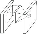
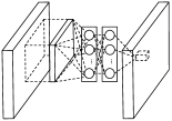
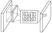
(a) convolutional layer	(b) Mlpconv layer	(c) Quanvolutional layer	(d) QFE layer

Figure 1: Comparison of convolutional layer, mlpconv layer, quanvolutional layer and QFE layer. The convolutional layer includes a linear filter. The mlpconv layer includes a multilayer perceptron. The quanvolutional layer includes a random quantum circuit without trainable parameters. The QFE layer includes a “micro quantum network”(we choose PQC in this paper).

III Convolutional Network with Quantum Feature Extraction Layers

In this section, we will first describe the quantum-classical hybrid model with quantum feature extraction layers and give a training algorithm. Then the possible experimental setup for its realization is discussed.

III.1 Quantum Feature Extraction Layers

A quantum feature extraction(QFE) layer is a transformational layer using learnable parameteried quantum circuits. It is similar to a convolutional layer in classical CNNs. Combining pooling layers, fully-connected layer even with convolutional layer, we can construct a hybrid quantum-classical neural network.

Suppose a QFE layer learns a mapping $F$, which conceptually consists of three parts, namely encoding, variational evolution, decoding.

1. Encoding. This operation encodes patches from the input data $\bm{x}$(or the output of previous layer) into a quantum circuit by applying $U_{en}(\bm{x})$ to the initialized states $|0\rangle^{n}$. Hereafter, we abbreviate $|0\rangle^{n}$ as $|0\rangle$ if there is no confusion. Note that the output state $|\bm{x}\rangle$ are characterized by input $x$.

2. Variational evolution. In this part, we apply a parameterized unitary circuit $U_{var}(\bm{\theta})$ to the quantum state $|x\rangle$. $U_{var}(\bm{\theta})$ maps the quantum state $|\bm{x}\rangle$ onto another quantum state $|\bm{x};\bm{\theta}\rangle$ using a serial of quantum gates. This operation can introduce quantum properties such as superposition, entanglement and quantum parallelism.

3. Decoding. This operation include two parts: measurement and classical post-processing. Firstly, at the end of the circuit, measurements are performed on an observable $\hat{H}$ to get an expectation value. Then after the classical post-processing, we get a output of one step in QFE layer. Analogously to a classical convolution layer, each output is mapped to a different channel of a single pixel value.

The structure of a QFE layer is compared with convolutional , quanvolutional and mlpconv layer in Fig. 1. Next we detail our definition of each operation.

III.1.1 Encoding

There are two popular strategy to encode classical data into quantum circuit, including the basis encoding and the amplitude encoding. The basis encoding method treats two basic states of a qubit, $|0\rangle$ and $|1\rangle$, as binary values of a classical bit, 0 and 1. While the amplitude encoding method uses the probability amplitudes of a quantum state to store classical data. As described below, to update the parameters effectively, we need to calculate the partial derivative of input. However, the two methods mentioned above are difficult to achieve it. To satisfy the condition, we treat a single input value as the angle of a parametrized rotation gate. Combining with parameter-shift rulemitarai2018quantum , we can calculate the analytical gradients of input on quantum circuits. Formally, the encoding part is expressed as an operation $F_{1}$:

$$F_{1}(\bm{x})=U_{en}(\bm{x})|0\rangle=|\bm{x}\rangle.$$ (4)

Here $\bm{x}=(x_{1},x_{2},\dots,x_{n})^{\bm{T}}$ is the input patch of QFE layer where $n$ is the dimension of $\bm{x}$(usually in a $3\times 3$ or $5\times 5$ size) and represents the size of the quantum circuit. $U_{en}(\bm{x})$ is a unitary to embed $\bm{x}$ into a quantum circuit. For example, as we used in the experiments, $U_{en}(\bm{x})$ can expressed as:

$$U_{en}(\bm{x})=\bigotimes_{i=1}^{n}R_{y}(x_{i}).$$ (5)

III.1.2 Variational evolution

The first part encodes the each of input patch $\bm{x}$ as a quantum state $|\bm{x}\rangle$. In the second part, applying a unitary $U_{var}(\bm{\theta})$, we map the state $|\bm{x}\rangle$ into another state $|\bm{x};\bm{\theta}\rangle$. Utilizing the power of quantum mechanics, such as superposition and entanglement, we hope that it can improve the usefulness of features. The operation of the second part is:

$$F_{2}(\bm{x})=U_{var}(\bm{\theta})|\bm{x}\rangle=|\bm{x};\bm{\theta}\rangle,$$ (6)

where $U(\bm{\theta})$ is an ansatz characterized by the parameters $\theta$ and $\theta$ is a vector whose dimension depends on the type of ansatz. It is important to find an expressive ansatz that can achieve a big range of quantum states. More generally, it is possible to repeat $U_{var}(\bm{\theta})$ to reach more quantum states. But this can increase the complexity of the model, and thus demands more training time.

In order to implement the ansatz in a real quantum device, we select $\{H,R_{X},R_{Y},R_{Z},CNOT\}$ to compose the ansatz In this case, motivated by the universality of QAOA lloyd2018quantum ; morales2020universality , we use a QAOA-heuristic circuit as an ansatz. The circuit is as shown in Fig. 2.

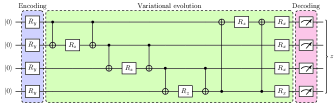
Figure 2: The QAOA-heuristic circuit.

III.1.3 Decoding

To access the information of the quantum states, we need to “decode” the quantum state $|\bm{x};\bm{\theta}\rangle$ into classical data, which consists of measurement and classical post-processing. At the measurement part, we measure a expectation value of a observable $\hat{H}$. Then, in classical post-processing part, we transform this expectation value to get the output by adding a bias $b$. The output is expressed as:

$$F_{3}(\bm{x})=\sigma(Tr(|\bm{x};\bm{\theta}\rangle\langle\bm{x};\bm{\theta}|\hat{H})+b),$$ (7)

where $|\bm{x};\bm{\theta}\rangle$ is the output state from the variational evolution part and $b$ is the bias. $\hat{H}$ is an observable composed of $\{\hat{H_{k}}\}_{k=1}^{l}$ where $H_{k}$ is a fixed Hamiltonian. $Tr(\cdot)$ is the trace operator. $\sigma(\cdot)$ is the activation function. Its function is to manipulate the outputs into a range of $[0,2\pi]$

III.2 Backward pass of QFE layer

In classical NNs, gradient descent based optimization algorithms are usually applied to update the parameters. A powerful routine in training is the backpropagation algorithm, which combines the chain rule for derivatives and stored values from intermediate layers to efficiently compute gradients. However, this strategy can not generalized straightforwardly to the QFE layer, because intermediate values from a quantum circuit can only be accessed via measurements, which will cause the collapse of quantum states. Using the parameter-shift rule and the chain rule, we proposed a training algorithm to compute the gradients of QFE Layer which can be embedded in the standard backpropagation. Hence we can train the hybrid model as a whole.

Suppose a QFE layer with parameters $\bm{\theta}$, $b$, whose input is $Z$ and output is $A$. The size of $Z$ is $m\times m$. The size of kernel is $f\times f$ and the stride is $s$, therefore, the size of $A$ is $(\lfloor\frac{m-f}{s}\rfloor+1)\times(\lfloor\frac{m-f}{s}\rfloor+1)$. Let $n=\lfloor\frac{m-f}{s}\rfloor+1$ to make the procedure clearer. Then, $Z$ and $A$ can be expressed as:

$$Z=\begin{pmatrix}z_{11}&z_{12}&\cdots&z_{1m}\\ z_{21}&z_{22}&\cdots&z_{2m}\\ \vdots&\vdots&\ddots&\vdots\\ z_{m1}&z_{m2}&\cdots&z_{mm}\end{pmatrix},$$ (8)

$$A=\begin{pmatrix}a_{11}&a_{12}&\cdots&a_{1n}\\ a_{21}&a_{22}&\cdots&a_{2n}\\ \vdots&\vdots&\ddots&\vdots\\ a_{n1}&a_{n2}&\cdots&a_{nn}\end{pmatrix}.$$ (9)

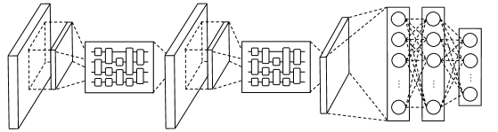
(a) The model that includes the stacking of two QFE layers and a classical “classifier”.

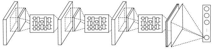
(b) The model that includes the stacking of three QFE layers and a global average layer.

Figure 3: The overall structures of evaluated models.

$L$ denotes the loss function. Firstly, consider the condition $s=1$ which is be commonly used. Assuming that the partial derivative $\frac{\partial L}{\partial A}$ was known. $\frac{\partial a_{ij}}{\partial z_{uv}}$ and $\frac{\partial a_{ij}}{\partial\theta_{k}}$ where $i,j=1,\cdots,n$, $u,v=1,\cdots,m$ and $k=1,\cdots,l$ can be calculated by parameter-shift rule. To implement the backpropagation of the QFE layer, we need to get $\frac{\partial L}{\partial\bm{\theta}}$, $\frac{\partial L}{\partial b}$ and $\frac{\partial L}{\partial Z}$. For convenience, we flatten $\frac{\partial L}{\partial Z}$ and $\frac{\partial L}{\partial A}$ row by row as follow:

$$\frac{\partial L}{\partial A}=\begin{pmatrix}\frac{\partial L}{\partial a_{11}}&\cdots&\frac{\partial L}{\partial a_{1n}}\\ \frac{\partial L}{\partial a_{21}}&\cdots&\frac{\partial L}{\partial a_{2n}}\\ \vdots&\ddots&\vdots\\ \frac{\partial L}{\partial a_{n1}}&\cdots&\frac{\partial L}{\partial a_{nn}}\\ \end{pmatrix}\rightarrow\frac{\partial L}{\partial\overline{A}}=\begin{pmatrix}\frac{\partial L}{\partial\overline{a}_{1}}\\ \frac{\partial L}{\partial\overline{a}_{2}}\\ \vdots\\ \frac{\partial L}{\partial\overline{a}_{n\times n}}\end{pmatrix}.$$ (10)

For $\frac{\partial L}{\partial b}$, by the chain rule, we have

$$\frac{\partial L}{\partial b}=\sum_{i,j}\frac{\partial a_{i,j}}{\partial b}\frac{\partial L}{\partial a_{i,j}}=\sum_{i,j}\frac{\partial L}{\partial a_{i,j}}=\sum\frac{\partial L}{\partial A}.$$ (11)

For $\frac{\partial L}{\partial\bm{\theta}}$, by the chain rule, we have

$$\frac{\partial L}{\partial\theta_{k}} = \sum_{i=1}^{m}\sum_{j=1}^{m}\frac{\partial a_{ij}}{\partial\theta_{k}}\frac{\partial L}{\partial a_{ij}}=\sum_{i=1}^{m\times m}\frac{\partial\overline{a}_{i}}{\partial\theta_{k}}\frac{\partial L}{\partial\overline{a}_{i}}$$

$$= \begin{pmatrix}\frac{\partial\overline{a}_{1}}{\partial\theta_{k}}&\frac{\partial\overline{a}_{2}}{\partial\theta_{k}}&\cdots&\frac{\partial\overline{a}_{m\times m}}{\partial\theta_{k}}\end{pmatrix}\begin{pmatrix}\frac{\partial L}{\partial\overline{a}_{1}}\\ \frac{\partial L}{\partial\overline{a}_{2}}\\ \vdots\\ \frac{\partial L}{\partial\overline{a}_{m\times m}}\end{pmatrix}=\frac{\partial\overline{A}}{\partial\theta_{k}}^{T}\frac{\partial L}{\partial\overline{A}}.$$

Thus,

$$\frac{\partial L}{\partial\bm{\theta}}=\begin{pmatrix}\frac{\partial L}{\partial\theta_{1}}\\ \frac{\partial L}{\partial\theta_{2}}\\ \vdots\\ \frac{\partial L}{\partial\theta_{l}}\end{pmatrix}=\frac{\partial\overline{A}}{\partial\bm{\theta}}^{T}\frac{\partial L}{\partial\overline{A}},$$ (13)

where $\frac{\partial\overline{A}}{\partial\bm{\theta}}^{T}=\begin{pmatrix}\frac{\partial\overline{a}_{1}}{\partial\theta_{1}}&\frac{\partial\overline{a}_{2}}{\partial\theta_{1}}&\cdots&\frac{\partial\overline{a}_{m\times m}}{\partial\theta_{1}}\\ \frac{\partial\overline{a}_{1}}{\partial\theta_{2}}&\frac{\partial\overline{a}_{2}}{\partial\theta_{1}}&\cdots&\frac{\partial\overline{a}_{m\times m}}{\partial\theta_{2}}\\ \vdots&\vdots&\ddots&\vdots\\ \frac{\partial\overline{a}_{1}}{\partial\theta_{l}}&\frac{\partial\overline{a}_{l}}{\partial\theta_{1}}&\cdots&\frac{\partial\overline{a}_{m\times m}}{\partial\theta_{l}}\\ \end{pmatrix}$.

To compute the $\frac{\partial L}{\partial Z}$, we define $\frac{\partial A}{\partial Z}$ as

$$\frac{\partial A}{\partial Z}=\left(\begin{array}[]{cccc}\frac{\partial A}{\partial z_{11}}&\frac{\partial A}{\partial z_{12}}&\cdots&\frac{\partial A}{\partial z_{1m}}\\ \frac{\partial A}{\partial z_{21}}&\frac{\partial A}{\partial z_{22}}&\cdots&\frac{\partial A}{\partial z_{2m}}\\ \vdots&\vdots&\ddots&\vdots\\ \frac{\partial A}{\partial z_{m1}}&\frac{\partial A}{\partial z_{m2}}&\cdots&\frac{\partial A}{\partial z_{mm}}\\ \end{array}\right),$$ (18)

where $\frac{\partial A}{\partial z_{ij}}=\begin{pmatrix}\frac{\partial a_{11}}{\partial z_{ij}}&\frac{\partial a_{12}}{\partial z_{ij}}&\cdots&\frac{\partial a_{1n}}{\partial z_{ij}}\\ \frac{\partial a_{21}}{\partial z_{ij}}&\frac{\partial a_{22}}{\partial z_{ij}}&\cdots&\frac{\partial a_{2n}}{\partial z_{ij}}\\ \vdots&\vdots&\ddots&\vdots\\ \frac{\partial a_{n1}}{\partial z_{ij}}&\frac{\partial a_{n2}}{\partial z_{ij}}&\cdots&\frac{\partial a_{nn}}{\partial z_{ij}}\\ \end{pmatrix}$.

Then, the $\frac{\partial L}{\partial Z}$ can be expressed as

$$\frac{\partial L}{\partial Z}=\frac{\partial A}{\partial Z}*\frac{\partial L}{\partial A},$$ (19)

where ‘$*$’ denotes the convolution operation with the stride $n$.

IV Experiments

In this section, we measure the performance of our hybrid models on MNIST lecun1998gradient dataset by numerical simulations. All of the experiments are performed with Yao luo2020yao package in Julia language.

IV.1 Dataset

The MNIST dataset is composed of 10 classes of hand written digits 0-9. There are 60,000 training images and 10,000 testing images. Each image is a gray image of size $28\times 28$. To save the training time, we cut the images into $22\times 22$ without information loss, as the original images are $20\times 20$. For training and testing procedure, we use 6000 and 600 samples of all categories evenly for training set and test set, respectively. The labels use one-hot encoding.

IV.2 Effectiveness of proposed method

Architecture selection: Here, to verify the feasibility of the scheme, we evaluated models of following architectures. The models all consist of stacked QFE layers instead of linear convolutional layers.

1. QFE layers with fully-connected layers. A model, which is similar to the classical CNN, replaces the linear convolutional layers with QFE layers. The structure is as followed: QFE1 - POOL1 - QFE2 - POOL2 - FC1 - FC2 - FC3. As shown in the Fig. 3(a) In this model, the fully-connected layers work as a “classifier”. We regard this model as model 1.

2. QFE layers with global average pooling. A model uses global average pooling (GAP) instead of fully-connected layers at the top of the network, with following structure: QFE1 - POOL1- QFE2 - QFE3 - GAP. As shown in Fig. 3(b). In this case, GAP introduced as a regularizer in Ref. lin2013network is used to remove the “classical factors” of the network. We regard this model as model 2.

Each QFE layer uses “quantum filters” of size $3\times 3$. Max pooling is used in the pooling layers which downsamples the size of input by a factor of 2.

Training strategy: For fair comparison, we adopt the same dataset for training. To save training time, we also explore a step-by-step training procedure. First, we train the network from scratch with a relatively small dataset. Then when the training is saturated, we add more training data for fine-tuning and repeat this step. With this strategy, the training converges earlier and faster than training with the larger dataset from the beginning. For initialization, the weights of QFE layers are initialized by drawing randomly from a uniform distribution with a range of $[-\pi,\pi]$, while the weights of fully-connected layers are initialized by a Gaussian distribution with zero mean and standard deviation 0.001. The models are trained using Adam optimization algorithm with mini-batches of size 50. The initial learning rate is 0.01 and is adjusted manually during training.

IV.3 Investigation of different settings

To investigate the property of the model, we design a set of controlling experiments with different settings of two variables - the type of the ansatz and the number of layers of ansatz, based on the structure of model 2 (i.e. QFE1 - POOL1- QFE2 - QFE3 - GAP).

IV.3.1 Type of ansatz

Recent work by Sim etc.sim2019expressibility studies expressibility the entangling capability of quantum circuits, showing these descriptors are related to the performance of PQCs-based algorithms. Here, we compare the model performance with different ansaetze. Specifically, we choose circuit 1, 2, 9, 14 and 15 in sim2019expressibility besides the QAOA-heuristic circuit.

IV.3.2 Number of layers

In general, the performance would improve if we increase the number of layers of ansatz at the cost of running time. Here, we examine the model sensitivity to different number of layers. In previous experiments, we set the number of layers of ansatz $L=3$ for each ”quantum” filter. To be consistent with previous experiments, we keep the kinds of ansaetze but change the number of layers from 1 to 5. All the other settings remain the same with model 2.

Totally, we examine 30 models for the same training data with 2560 samples for 9 epochs. The experimental setup is shown in the Table I.

Table 1: Experimental setup to investigate different settings

Epoch	Learning rate	batch size
1	0.01	32
2 - 3	0.005	32
4 - 6	0.001	32
7 - 9	0.0005	16

IV.4 Results

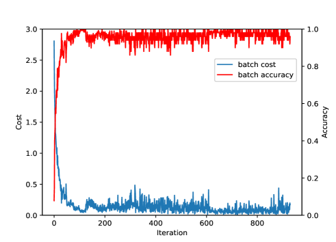
Figure 4: Training cost and accuracy for the model that includes QFE layers with fully-connected layers.

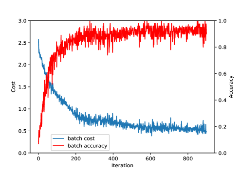
Figure 5: Training cost and accuracy for the model that includes QFE layers with GAP.

We first report results on classification to demonstrate that our method works with fully-connected layers or not. Then we compare the performance between different settings.

Classification. training performances between model 1 and model 2 are shown in Fig. 4 and Fig. 5. For test set error rates, model1 and model2 achieve 3.1% and 6.8% respectively. It is reasonable for the toy models. However, removing classical fully-connected layers, there is a small performance drop of 2 - 3%.

Compare using different settings. To further compare our approach with different settings mentioned above, we train the models with the same dataset and the results are shown in Fig.6. Note that these results are obtained using different ansaetze with different layers. We can observe that the model converges lower cost and achieves higher accuracy with deeper layers in ansatz. However, we note that “saturation” phenomenon exists, which means adding addition layers to PQC, the performance of the model does not always continue to improve. This phenomenon appears more and less in all of the ansaetze. Take circuit 9 as an example, the model with 2-layer PQC converges on a lower value and a higher accuracy than that with 1-layer PQC, while the curves of cost and accuracy are almost the same respectively, when the models equip with circuit 9 in 4 layers and 5 layers. The “saturation” phenomenon may relate with expressibility saturationsim2019expressibility or barren plateausmcclean2018barren . To understand how expressibility correlates with the model performance further, future research is needed.

This section aims to demonstrate a proof of concept for the proposed method on a real-world dataset. Because the training is time-consuming, we construct our architectures based on the small model which has only two or three layers. Note that model 2 which has no classical fully-connected layers achieves 6.8% test set error. This shows the the effectiveness of QFC layers and their training algorithm.

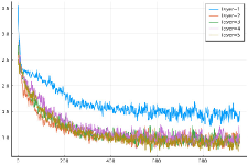
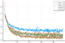
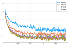
(a) costs of circuit 1	(c) costs of circuit 2	(e) costs of circuit 9
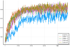
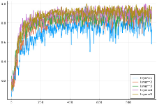
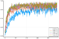
(b) accuracies of circuit 1	(d) accuracies of circuit 2	(f) accuracies of circuit 9
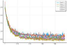
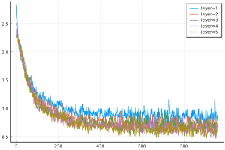
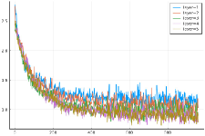
(g) costs of circuit 14	(i) costs of circuit 15	(k) costs of QAOA-like circuit
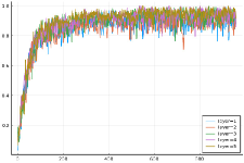
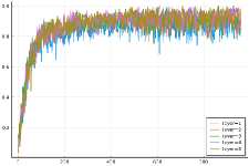
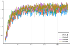
(h) accuracies of circuit 14	(j) accuracies of circuit 15	(l) accuracies of QAOA-like circuit

Figure 6: The performances (cost and accuracy) of models with different settings

V Conclusions

This paper proposed a hybrid quantum-classical network with deep architectures. The new structure consists of QFE layers which use PQCs to “convolve” the input. QFE layers generalize convolution to the high dimensional hilbert space and model the local patches better. It has been shown that our hybrid models can achieve competitive performances based on simple architectures. Besides, we compare the performances of models with different ansaetze in different depths, showing that the model with ansatz in high expressibility performs better. In practice, the network architecture and the initialization method have a significant impact on performance. However, there is a no effective method to avoid the barren plateaus yet. On the other hand, since the modern classical network are so deep and our method provides many possibilities via PQCs, we cannot perform exhaustive tests to find the best sequence of QFE layers and the best combination of circuit ansaetze. Due to the large number of choices of PQCs, we cannot perform a brute force search for all the possibilities, while this opens a new space for the construction of hybrid quantum-classical networks. We expect the introduction of QFE layers in more architectures and extensive hyperparameter searches can improve the performance.

Besides, it is noted that quantum neural tangent kernel (QNTK) theorynakaji2021quantum ; shirai2021quantum ; liu2021representation is developed recently, which can be applied to QNNs. It will be interesting to analyze the model with QFE layers based on the QNTK theory. This open question is left for future research.

- (1) F. Arute, K. Arya, R. Babbush, D. Bacon, J. C. Bardin, R. Barends, R. Biswas, S. Boixo, F. G. S. L. Brandao, D. A. Buell et al., Quantum supremacy using a programmable superconducting processor, Nature (London) 574, 505 (2019).
- (2) J. Preskill, Quantum computing in the NISQ era and beyond, Quantum 2, 79 (2018).
- (3) J. Biamonte, P. Wittek, N. Pancotti, P. Rebentrost, N. Wiebe, and S. Lloyd, Quantum machine learning, Nature (London) 549, 195 (2017).
- (4) P. Rebentrost, M. Mohseni, and S. Lloyd, Quantum Support Vector Machine for Big Data Classification, Phys. Rev. Lett. 113, 130503 (2014).
- (5) S. Lloyd, M. Mohseni, and P. Rebentrost, Quantum principal component analysis, Nat. Phys. 10, 631 (2014).
- (6) M. H. Amin, E. Andriyash, J. Rolfe, B. Kulchytskyy, and R. Melko, Quantum Boltzmann Machine, Phys. Rev. X 8, 021050 (2018).
- (7) A. Mari, T. R. Bromley, J. Izaac, M. Schuld, and N. Killoran, Transfer learning in hybrid classical-quantum neural networks, Quantum 4, 340 (2020).
- (8) V. Havlíček, A. D. Córcoles, K. Temme, A. W. Harrow, A. Kandala, J. M. Chow, and J. M. Gambetta, Supervised learning with quantum-enhanced feature spaces, Nature (London) 567, 209 (2019).
- (9) M. Schuld and N. Killoran, Quantum Machine Learning in Feature Hilbert Spaces, Phys. Rev. Lett. 122, 040504 (2019).
- (10) M. Benedetti, E. Lloyd, S. Sack, and M. Fiorentini, Parameterized quantum circuits as machine learning models, Quantum Sci. Technol. 4, 043001 (2019).
- (11) P. W. Shor, Polynomial-time algorithms for prime factorization and discrete logarithms on a quantum computer, SIAM Rev. 41, 303 (1999).
- (12) L. K. Grover, Quantum Mechanics Helps in Searching for a Needle in a Haystack, Phys. Rev. Lett. 79, 325 (1997).
- (13) A. W. Harrow, A. Hassidim, and S. Lloyd, Quantum Algorithm for Linear Systems of Equations, Phys. Rev. Lett. 103, 150502 (2009).
- (14) A. Peruzzo, J. McClean, P. Shadbolt, M.-H. Yung, X.-Q. Zhou, P. J. Love, A. Aspuru-Guzik, and J. L. O’Brien, A variational eigenvalue solver on a photonic quantum processor, Nat. Commun. 5, 4213 (2014).
- (15) D. Wecker, M. B. Hastings, and M. Troyer, Progress towards practical quantum variational algorithms, Phys. Rev. A 92, 042303 (2015).
- (16) J. R. McClean, J. Romero, R. Babbush, and A. Aspuru-Guzik, The theory of variational hybrid quantum-classical algorithms, New J. Phys. 18, 023023 (2016).
- (17) E. Farhi, J. Goldstone, and S. Gutmann, A quantum approximate optimization algorithm, arXiv:1411.4028.
- (18) S. Hadfield, Z. Wang, B. O’Gorman, E. G. Rieffel, D. Venturelli, and R. Biswas, From the quantum approximate optimization algorithm to a quantum alternating operator ansatz, Algorithms 12, 34 (2019).
- (19) M. Schuld, I. Sinayskiy, and F. Petruccione, The quest for a quantum neural network, Quantum Inf. Process. 13, 2567 (2014).
- (20) E. Farhi and H. Neven, Classification with quantum neural networks on near term processors, arXiv:1802.06002.
- (21) S. Lloyd, M. Schuld, A. Ijaz, J. Izaac, and N. Killoran, Quantum embeddings for machine learning, arXiv:2001.03622.
- (22) I. Cong, S. Choi, and M. D. Lukin, Quantum convolutional neural networks, Nat. Phys. 15, 1273 (2019).
- (23) M. Henderson, S. Shakya, S. Pradhan, and T. Cook, Quanvolutional neural networks: powering image recognition with quantum circuits, Quantum Machine Intelligence 2, 1 (2020).
- (24) I. Kerenidis, J. Landman, and A. Prakash, Quantum algorithms for deep convolutional neural networks, In Proceedings of the International Conference on Learning Representations (ICLR, Addis Ababa, Ethiopia, 2020).
- (25) Y.-C. Li, R.-G. Zhou, R.-Q. Xu, J. Luo, and W.-W. Hu, A quantum deep convolutional neural network for image recognition, Quantum Sci. Technol. 5, 044003 (2020).
- (26) H. Zheng, Z. Li, J. Liu, S. Strelchuk, and R. Kondor, Speeding up learning quantum states through group equivariant convolutional quantum ans ” a tze, arXiv:2112.07611.
- (27) M. Lin, Q. Chen, and S. Yan, Network in network, In Proceedings of the International Conference on Learning Representations (ICLR, Banff, AB, Canada, 2014).
- (28) M. Schuld, R. Sweke, and J. J. Meyer, Effect of data encoding on the expressive power of variational quantum machine learning models, Phys. Rev. A 103, 032430 (2021).
- (29) T. Goto, Q. H. Tran, and K. Nakajima, Universal Approximation Property of Quantum Machine Learning Models in Quantum-Enhanced Feature Spaces, Phys. Rev. Lett. 127, 090506 (2021).
- (30) J. Liu, K. H. Lim, K. L. Wood, W. Huang, C. Guo, and H.-L. Huang, Hybrid quantum-classical convolutional neural networks, Sci. China Phys. Mech. Astron. 64, 290311 (2021).
- (31) Y. LeCun, B. Boser, J. S. Denker, D. Henderson, R. E. Howard, W. Hubbard, and L. D. Jackel, Backpropagation applied to handwritten zip code recognition, Neural Comput. 1, 541 (1989).
- (32) Y. LeCun, L. Bottou, Y. Bengio, and P. Haffner, Gradient-based learning applied to document recognition, Proc. IEEE 86, 2278 (1998).
- (33) A. Krizhevsky, I. Sutskever, and G. E. Hinton, Imagenet classification with deep convolutional neural networks, In Advances in Neural Information Processing Systems (NeurIPS, Lake Tahoe, NV, USA, 2012), pp. 1097-1105.
- (34) J. Redmon, S. Divvala, R. Girshick, and A. Farhadi, You only look once: Unified, real-time object detection, In Proceedings of the IEEE Conference on Computer Vision and Pattern Recognition (CVPR, Las Vegas, NV, USA, 2016), pp. 779-788.
- (35) J. Long, E. Shelhamer, and T. Darrell, Fully convolutional networks for semantic segmentation, In Proceedings of the IEEE Conference on Computer Vision and Pattern Recognition (CVPR, Boston, MA, USA, 2015), pp. 3431-3440.
- (36) L. Zhang, L. Lin, X. Liang, and K. He, Is faster R-CNN doing well for pedestrian detection?, In European Conference on Computer Vision (ECCV, Amsterdam, The Netherlands, 2016), pp. 443-457.
- (37) A. Vaswani, N. Shazeer, N. Parmar, J. Uszkoreit, L. Jones, A. N. Gomez, Ł. Kaiser, and I. Polosukhin, Attention is all you need, In Advances in Neural Information Processing Systems (NeurIPS, Long Beach, CA, USA, 2017), pp. 5998-6008.
- (38) C. Szegedy, W. Liu, Y. Jia, P. Sermanet, S. Reed, D. Anguelov, D. Erhan, V. Vanhoucke, and A. Rabinovich, Going deeper with convolutions, In Proceedings of the IEEE Conference on Computer Vision and Pattern Recognition (CVPR, Boston, MA, USA, 2015), pp. 1-9.
- (39) K. Simonyan and A. Zisserman, Very deep convolutional networks for large-scale image recognition, In Proceedings of the International Conference on Learning Representations (ICLR, San Diego, CA, USA, 2015).
- (40) K. He, X. Zhang, S. Ren, and J. Sun, Deep residual learning for image recognition, In Proceedings of the IEEE Conference on Computer Vision and Pattern Recognition (CVPR, Las Vegas, NV, USA, 2016), pp. 770-778.
- (41) G. Huang, Z. Liu, L. V. D. Maaten, and K. Q. Weinberger, Densely connected convolutional networks, In Proceedings of the IEEE Conference on Computer Vision and Pattern Recognition (CVPR, Honolulu, HI, USA, 2017), pp. 2261-2269.
- (42) P.-L. Dallaire-Demers and N. Killoran, Quantum generative adversarial networks, Phys. Rev. A 98, 012324 (2018).
- (43) J. Romero, J. P. Olson, and A. Aspuru-Guzik, Quantum autoencoders for efficient compression of quantum data, Quantum Sci. Technol. 2, 045001 (2017).
- (44) K. Sharma, S. Khatri, M. Cerezo, and P. J. Coles, Noise resilience of variational quantum compiling, New J. Phys. 22, 043006 (2020).
- (45) K. Mitarai, M. Negoro, M. Kitagawa, and K. Fujii, Quantum circuit learning, Phys. Rev. A 98, 032309 (2018).
- (46) S. Lloyd, Quantum approximate optimization is computationally universal, arXiv:1812.11075.
- (47) M. E. S. Morales, J. D. Biamonte, and Z. Zimborás, On the universality of the quantum approximate optimization algorithm, Quantum Inf. Process. 19, 291 (2020).
- (48) X.-Z. Luo, J.-G. Liu, P. Zhang, and L. Wang, Yao. jl: Extensible, efficient framework for quantum algorithm design, Quantum 4, 341 (2020).
- (49) S. Sim, P. D. Johnson, and A. Aspuru-Guzik, Expressibility and entangling capability of parameterized quantum circuits for hybrid quantum-classical algorithms, Adv. Quantum Technol. 2, 1900070 (2019).
- (50) J. R. McClean, S. Boixo, V. N. Smelyanskiy, R. Babbush, and H. Neven, Barren plateaus in quantum neural network training landscapes, Nat. Commun. 9, 4812 (2018).
- (51) K. Nakaji, H. Tezuka, and N. Yamamoto, Quantum-enhanced neural networks in the neural tangent kernel framework, arXiv:2109.03786.
- (52) N. Shirai, K. Kubo, K. Mitarai, and K. Fujii, Quantum tangent kernel, arXiv:2111.02951.
- (53) J. Liu, F. Tacchino, J. R. Glick, L. Jiang, and A. Mezzacapo, Representation learning via quantum neural tangent kernels, arXiv:2111.04225.