Propagation and attenuation of pulses driven by low velocity normal impacts in granular media

Abstract

We carry out experiments of low velocity normal impacts into granular materials that fill an approximately cylindrical 42 litre tub. Motions in the granular medium are tracked with an array of 7 embedded accelerometers. Longitudinal pulses excited by the impact attenuate and their shapes broaden and become smoother as a function of travel distance from the site of impact. Pulse propagation is not spherically symmetric about the site of impact. Peak amplitudes are about twice as large for the pulse propagating downward than at 45 degrees from vertical. An advection-diffusion model is used to estimate the dependence of pulse properties as a function of travel distance from the site of impact. The power law forms for pulse peak pressure, velocity and seismic energy depend on distance from impact to a power of -2.5 and this rapid decay is approximately consistent with our experimental measurements. Our experiments support a seismic jolt model, giving rapid attenuation of impact generated seismic energy into rubble asteroids, rather than a reverberation model, where seismic energy slowly decays. We apply our diffusive model to estimate physical properties of the seismic pulse that will be excited by the forthcoming DART mission impact onto the secondary, Dimorphos, of the asteroid binary (65803) Didymos system. We estimate that the pulse peak acceleration will exceed the surface gravity as it travels through the asteroid.

1 Introduction

Apollo-class Near-Earth Asteroid binary (65803) Didymos is the target of the international collaboration known as AIDA (abbreviation for Asteroid Impact & Deflection Assessment) that supports the development and data interpretation of the NASA’s Double Asteroid Redirection Test (DART) mission (Cheng et al., 2018; Rivkin et al., 2021) and the European Space Agency’s Hera mission (Michel et al., 2022). Goals of these missions to the potentially hazardous binary asteroid Didymos include measuring the momentum transfer efficiency and resulting deflection from a hyper-velocity asteroid impact. DART will be the first high-speed impact experiment on an asteroid at a scale relevant for planetary defense. Imaging during the impact will be carried out by the accompanying 6U CubeSat named the Light Italian CubeSat for Imaging of Asteroids (also known as LICIACube; Dotto et al. 2021).

A high velocity impact compresses the target material to high pressures, launching a shock wave which causes vaporization, melting, fragmentation, plastic deformation, and formation of a crater (Melosh, 1989). The expanding shock wave propagates outward from the impact site and attenuates as it propagates. When the velocity of the shock drops below a certain threshold, it continues to propagate as an elastic wave (Holsapple, 1993). Most Near Earth Asteroids (NEAs) are expected to be comprised of rubble (Walsh, 2018) which complicates predicting the strength and attenuation rate of impact induced seismic energy (McGarr et al., 1969).

There are two views on how impact generated seismic energy propagates within rubble asteroids (Cintala et al., 1978; Cheng et al., 2002; Richardson et al., 2004; Thomas and Robinson, 2005; Yamada et al., 2016). The rapidly attenuated seismic pulse or ‘jolt’ model (Nolan et al., 1992; Greenberg et al., 1994, 1996; Nolan et al., 2001; Thomas and Robinson, 2005) is consistent with strong attenuation in dry laboratory granular materials at kHz frequencies (Hostler and Brennen, 2005; O’Donovan et al., 2016). However, the jolt model qualitatively differs from the slowly attenuating seismic reverberation model (Cintala et al., 1978; Cheng et al., 2002; Richardson et al., 2004, 2005; Yamada et al., 2016), that is supported by measurements of slow seismic attenuation rates in lunar regolith (Dainty et al., 1974; Toksöz et al., 1974; Nakamura, 1976). While both impact-induced seismic jolt and reverberation can cause crater erasure, crater rim degradation and resurfacing (Veverka et al., 2001; Nolan et al., 2001; Richardson et al., 2004, 2005; Thomas and Robinson, 2005; Asphaug, 2008; Yamada et al., 2016), size segregation induced by the Brazil-nut effect could depend on sustained vibrations or reverberation (e.g., Miyamoto et al. 2007; Tancredi et al. 2012; Matsumura et al. 2014; Tancredi et al. 2015; Perera et al. 2016; Maurel et al. 2017; Chujo et al. 2018), though a single seismic pressure pulse can also leave boulders on the surface (Wright et al., 2020) via ballistic sorting (Shinbrot et al., 2017).

Pulse propagation in granular media is nonlinear, sensitive to pulse duration and amplitude, ambient or hydrostatic pressure and the nature of contacts in the granular medium (e.g., Goddard 1990; Liu and Nagel 1992; Jia et al. 1999; Johnson et al. 2000; Hostler and Brennen 2005; Bi et al. 2011; Gómez et al. 2012). At low pulse amplitude, the pulse propagation speed along the fastest travel path along one chain of contacts can differ from the propagation speed of a pulse peak (Liu and Nagel, 1992; Owens and Daniels, 2011). In some regimes, a pulse can propagate as if it were a coherent elastic wave or sound wave (Geng et al., 2003; Somfai et al., 2005; van den Wildenberg et al., 2013; Santibanez et al., 2016), while in other regimes, diffusive, dispersive and anisotropic behavior is predicted or observed (Da Silva and Rajchenbach, 2000; Otto et al., 2003; Jia, 2004; Luding, 2005; Hostler and Brennen, 2005). Hertzian (or Hertz-Mindlin) contact theory underlies estimates for the nature of sound propagation in granular media (e.g., Gómez et al. 2012; van den Wildenberg et al. 2013) and development of a continuum model, denoted an effective medium theory (e.g., Goddard 1990; Johnson et al. 2000). In granular systems, broadening and attenuation of seismic or acoustic pulses may be intrinsically related (Jia, 2004; Langlois and Jia, 2015; O’Donovan et al., 2016; Zhai et al., 2020).

The difficulty of predicting impact induced seismicity in granular systems has motivated experiments that measure the response of granular materials to impacts. McGarr et al. (1969) conducted impact experiments on epoxy-bonded sand and on unconsolidated or loose sand at impact velocities of 0.8 to 7 km/s. They measured accelerations using accelerometers placed on the substrate or target surface. The signals from the bonded sand experiment were sinusoidal, showing many periods of oscillation, however, the accelerations in the unconsolidated sand resembled a single period of a sine wave (see their Figure 3). Yasui et al. (2015) carried out a series of intermediate impact velocity experiments, with impact velocity approximately 100 m/s into spherical glass beads with diameter 180–250 $\mu$m. Matsue et al. (2020) extended this work with impact experiments into quartz sand at higher velocities ranging from 200 m/s to 7 km/s. The accelerometer signals from these two sets of experiments resembled those seen by McGarr et al. (1969) in unconsolidated sand, confirming that a single seismic pulse tends to be excited in a granular substrate by an impact. Yasui et al. (2015) and Matsue et al. (2020) showed that the strength of the peak acceleration $g_{max}$ in the impact generated seismic signal decayed as a function of distance $r$ from impact site with a power law function $g_{max}\propto r^{\gamma}$ with exponent $\gamma=-2.21\pm 0.12$ (Yasui et al., 2015) and $-3.12\pm 0.10$ (Matsue et al., 2020).

In this paper, using an array of 7 accelerometers, we examine how impact excited pulses travel in granular media. Our impacts are low velocity (a few m/s) normal impacts of small spherical projectiles into 41.6 litres of sand or millet contained in an approximately cylindrical tub. Our experiments are at lower velocity than those of Yasui et al. (2015) and Matsue et al. (2020) and we go beyond theses studies by comparing the impact generated seismic pulses in different granular substrates. We use our accelerometer array to study variations in the signal shapes as a function of depth and distance from impact. Our experiments are described in Section 2. In Section 3 we examine the peak values and durations of pulses and how the pulses propagate through the granular medium. Motivated by the rapid attenuation and smoothing and broadening of the pulse shapes, in Section 4 we use a diffusive attenuation model to study the dependence of pulse duration, peak amplitude and other quantities on distance from impact site. The DART impact gives unprecedented opportunity to probe how a seismic wave generated by a hypervelocity impact is transmitted through asteroid granular material and affects the surface. In Section 5 we discuss implications of our experiments and model for the forthcoming DART mission impact. A summary and discussion follow in Section 6.

Table 1: Accelerometer placement coordinates $(R,\theta,z)$

	A	B	C	D	E	F	G
L5	(5,0,-5)	(8,0,-5)	(11,0,-5)	(14,0,-5)	(17,0,-5)	(20,0,-5)	(23,0,-5)
L10 ​​	(2,0,-10)	(5,0,-10)	(8,0,-10)	(11,0,-10)	(14,0,-10)	(17,0,-10)	(20,0,-10)
L15 ​​	(2,0,-15)	(5,0,-15)	(8,0,-15)	(11,0,-15)	(14,0,-15)	(17,0,-15)	(20,0,-15)
R5	(5.5,-60,-4)	(5.5,-40, -7)	(5.5,-20, -10)	(5.5,0,-13)	(5.5,20,-16)	(5.5,40,-19)	(5.5,60,-22)
R10 ​​	(10.5,-45,-4)	(10.5,-30, -7)	(10.5,-15, -10)	(10.5,0,-13)	(10.5,15,-16)	(10.5,30,-19)	(10.5,45,-22)
R15 ​​	(15.5,-45,-4)	(15.5,-30, -7)	(15.5,-15, -10)	(15.5,0,-13)	(15.5,15,-16)	(15.5,30,-19)	(15.5,45,-22)

Notes: Each row gives a set or template of accelerometer coordinates. These are cylindrical coordinates $(R,\theta$,z), for each accelerometer with $R,z$ in cm and $\theta$ in degrees. The impact point is near the origin and on the surface. The column heads refer to the oscilloscope channels and the eighth or H oscilloscope channel is used to trigger data recording with the IR break-beam sensor. The coordinate locations refer to the position of the accelerometer ADXL335 integrated circuit. The angles are crudely estimated and should not affect the measurements because of the cylindrical symmetry of our experiment.

Figure 1: A side view illustration of the experiment, including the washtub, granular material, spherical impactor and accelerometer array. The unit vectors $\hat{\bf R},\hat{\bf z}$ are cylindrical coordinate directions with respect to the impact point.

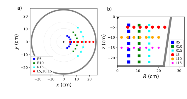
Figure 2: Illustration of the accelerometer placements. a) A top down view of the accelerometer positions. The thick grey circle shows the outline of the rim of the tub. Each coordinate template consists of 7 accelerometer positions and is shown with a different color and size marker. The coordinate templates are listed in Table 1. The point of impact is shown with a black dot at the origin. b) Similar to a) except showing a side view and plotting cylindrical radius $R$ vs $z$. The thick grey line shows the outline of the tub. The substrate surface is at $z=0$.

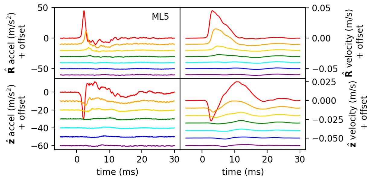
Figure 3: Accelerations measured in a 7 channel accelerometer array as a function of time following an impact for experiment ML5 into millet. The accelerometers are at the same depth and in a line with increasing distance from the impact site (the L5 coordinate template in Table 1). The top panels show the radial $\hat{\bf R}$ (cylindrical radius) components of acceleration and velocity and the bottom two panels show the vertical, $\hat{\bf z}$, components. The left two panels show acceleration and the right two panels show velocities. Signals from 7 accelerometers are plotted in each panel with a vertical offset between channels that is 10 m/s² for accelerations and 0.01 m/s for velocities. In all panels the plots are shown in order of distance from the impact site with the topmost signal from the accelerometer nearest the impact site. Each accelerometer is shown with a different color line.

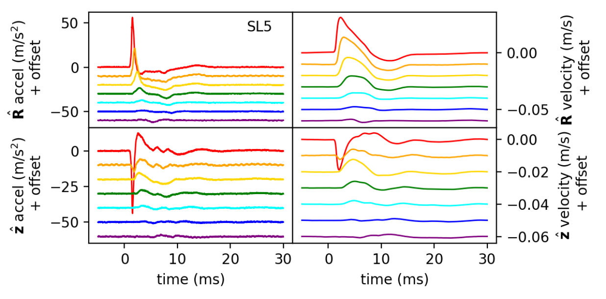
Figure 4: Similar to Figure 3 except showing the SL5 experiment with the same coordinate template but into fine sand. The pulse is narrower in this experiment than the similar ML5 experiment into millet.

2 Experimental Methods

Our granular substrate is held in a large 41.6 litre (11 gallon) washtub that is 25 cm deep and 52 cm in diameter at the top. The tub base is a circle with a diameter of 45 cm. The tub is filled with millet or sand. For an illustration of our experimental setup see Figure 1.

2.1 The array of accelerometers

We measure the impulse caused by an impact using an array of 7 accelerometers that are embedded within the granular substrate. The accelerometers are 5V-ready analog break-out boards by Adafruit which house the $\pm 3g$ triple-axis accelerometer ADXL335 Analog devices integrated circuit. The dimensions of the accelerometer printed circuit boards (PCBs) are 19 mm $\times$ 19 mm $\times$ 3 mm. The ADXL335 specifications describe its $z$ axis as that parallel to the narrowest dimension of the integrated circuit (and perpendicular to the PCB) and $x,y$ axes in the direction parallel to its two longer dimensions (and in the plane of the PCB). We removed three on-board filter capacitors from the PCB to increase the output bandwidth upper limit from 50 Hz to 1600 Hz on $x$- and $y$-axes and to 550 Hz on the $z$-axis. We only use the $x$ and $y$ axis accelerometer signals because they have a higher bandwidth upper limit. The bandpass upper limits are frequencies at which the signal amplitude is reduced by 3 dB (the amplitude drops by a factor of 0.5) and approximately equal to the cutoff frequency of a low pass filter. The 1600 Hz bandwidth upper limit correspond to a half period of 0.3 ms which is shorter than the width of the acceleration pulses seen in our experiments. So that the accelerometers are free to move within the media, we used fine and flexible 36 AWG gauge wire to power the accelerometers and connect their signal outputs.

Each accelerometer was individually calibrated in each axis by placing it on a level surface, taking a measurement, rotating it by $180^{\circ}$ around a horizontal axis and then repeating the measurement. The difference between the two measured voltages are equivalent to 2 $g$, giving a calibration factor from volts to m/s². The calibration factors are within $\pm$ 0.002 V per m/s² of the mean value of all 7 accelerometers (that is $0.032\ V$ per m/s²). We also recorded the DC voltage of each axis when aligned horizontally. These were used to check the accelerometer orientations.

The output signals of the $x$ and $y$-axis outputs of the accelerometers were recorded with 8-channel digital oscilloscopes (Picoscope model 4824A) with a sampling rate of 100 kHz. We use a range for the oscilloscope channels of $\pm 5V$ for each accelerometer giving 0.07 m/s² of precision in the acceleration measurements.

2.2 Triggering

The impactors are solid spherical objects like a rubber ball or glass marble, that are released from a height of $h_{drop}\sim 1$ m above the substrate surface. A small iron washer is glued to the ball. The ball is held in place with a solenoid that releases the ball when the solenoid is disconnected from DC power. As the ball falls, it passes between the transmitter and receiver of an IR break-beam sensor pair and this triggers recording of the accelerometer signals. Rubber and glass are not perfectly opaque to infrared light and the projectiles surfaces can reflect light. To improve the accuracy of the trigger timing, we painted the projectile surfaces matte black with common oil paint. The two oscilloscopes are triggered to record 14 channels of accelerometer data at the same time. One oscilloscope is used to record the $x$-axis accelerometer outputs and the other is used to record the $y$-axis outputs. In each oscilloscope channels 1 to 7 (also denoted channels A through G) are used to record accelerometer data and the 8-th, or H-th, channel is used to trigger the recordings.

2.3 Accelerometer placement

Prior to each impact experiment we rake the substrate a few times, with a rake that has prongs that are about 10 cm long and are equally spaced by a cm. The rake is also used to level the surface. After raking, the accelerometers are embedded in the medium. We orient the accelerometers so that their $+x$ axes point away from the impact site and their $+y$ axes point vertically up. To ensure that the accelerometers are correctly spaced, at the desired depth, and correctly oriented, we individually placed each accelerometer in the medium. For the shallow depths (less than 5 cm), we used a pair of long tweezers. For the deeper locations we used a PVC tube with filed slots to hold the accelerometer board while we slowly pushed it into the granular medium. The DC voltage levels of each accelerometer were monitored in both axes during placement to ensure that their orientations are approximately consistent with the desired orientation. We compared the DC voltage levels of the accelerometer signals prior to impact to the calibration values and find that the accelerometers, once embedded, are typically within $10^{\circ}$ of the desired orientation.

We adopt a coordinate system with origin at the impact site. In Cartesian coordinates $(x,y,z)$ the vertical and $z$ coordinate is negative below the horizontal substrate surface. It is convenient to use a cylindrical coordinate system $(R,\theta,z)$ to describe accelerometer positions. Radius $R$ is the radial distance to the vertical line going through the impact point. The $z$ coordinate gives height from the initially flat granular surface. Directions for motions are described in terms of a radial unit vector in cylindrical coordinates $\hat{\bf R}=\frac{1}{R}(x,y,0)$, where on the right we write the vector in Cartesian coordinates, and a vertical unit vector $\hat{\bf z}=(0,0,1)$ (in either cylindrical coordinates or Cartesian coordinates). Since our accelerometers are below the surface we describe their vertical position in terms of a depth which is $-z$. Acceleration in the $+x$-axis direction with respect to the accelerometer chip gives measurements of acceleration in the radial $+\hat{\bf R}$ direction. Acceleration in the $+y$-axis direction with respect to the accelerometer chip gives measurements of acceleration in the vertical cylindrical coordinate or $+\hat{\bf z}$ direction. It is also convenient to use a spherical coordinate system to describe subsurface motions. The radius from the impact site $r=\sqrt{x^{2}+y^{2}+z^{2}}=\sqrt{R^{2}+z^{2}}$. The radial direction from the impact site is unit vector $\hat{\bf r}=\frac{1}{r}(x,y,z)$, where on the right we have the vector in Cartesian coordinates.

The 7 accelerometers were placed in the granular medium in sets of locations which we refer to as coordinate templates. The cylindrical coordinates of each accelerometer are listed in Table 1 for each coordinate template. Templates denoted with letter $L$ have accelerometers placed in a line, at different radii and all at the same depth. Templates denoted with letter $R$ have accelerometers all at the same cylindrical radius, but at different depths and polar angles.

Table 2: Properties of Spherical Projectiles

		Rubber	Glass
		Ball	Marble
Radius	$R_{p}$ (cm)	1.83	1.41
Mass	$m_{p}$ (g)	27.3	30.9
Density	$\rho_{p}$ (g cm-3)	1.06	2.63
Young’s modulus	$E_{p}$ (GPa)	$\sim\!$ 0.01	$\sim$ 50
Sound prop. velocity	$c_{p}$ (m/s)	$\sim\!$ 100	$\sim$ 4400
Sound prop. time	$t_{D,prop}$ (ms)	$\sim\!$ 0.7	$\sim$ 0.012

Notes: We measured the mass and radius of each projectile. The sound velocity is an estimate for that within the projectile and the sound propagation time is the time for a sound wave to traverse the object’s diameter twice.

2.4 Properties of granular media and impactors

Spherical impactor masses $m_{p}$ and radii $R_{p}$ are listed in Table 2. Impactors (which we also call projectiles) were chosen so that their density $\rho_{p}$ approximately matches that of the granular substrate. For the experiments in sand we used a green glass marble and for the experiments into millet we used a colorful rubber ball. This reduces sensitivity to the substrate to projectile density ratio that is present in crater scaling laws (Holsapple, 1993). For the projectiles we list rough estimates for their Young’s modulus $E_{p}$, sound propagation speed $c_{p}\approx\sqrt{E_{p}/\rho_{p}}$, and time for a sound wave to propagate back and forth across the projectile $t_{D,prop}=4R_{p}/c_{p}$.

The properties of the granular media are listed in Table 3. Millet has the advantage that it is low density and this facilitates placing accelerometers deep within the medium. Sand has the advantage that its grain properties are similar to rocky materials that might be present on planetary surfaces. The millet is white proso millet marketed as birdseed. The sand is the fine light playground sand described by Wright et al. (2022), and was passed through a sieve to remove particles greater than 0.5 mm in width. Both substrates are inexpensive. The procedures for measuring bulk density $\rho_{s}$, grain density $\rho_{g}$, porosity $\phi$, angle of repose $\theta_{r}$ and static friction coefficient $\mu_{s}$, are described by Wright et al. (2022). We adopt the Young’s modulus $E_{g}\approx 100$ MPa for millet grain material measured by Yang et al. (2015) using a Hertzian contact model. Sound speeds within the grains are estimated with $c_{g}\approx\sqrt{E_{g}/\rho_{g}}$. For sand grains we use the Young’s modulus of $E_{g}\sim 10$ GPa which gives a seismic p-wave velocity of about $c_{g}\sim 2$ km/s, similar to that in soft sandstones. We list typical grain axis lengths for the millet in Table 3. The millet seed sizes are fairly similar but they are not spherical. The fine sand has a wide grain size distribution, with a FWHM in the major axis distribution about 0.4 times the mean value (see Figure 3d by Wright et al. 2022).

Table 3: Properties of Granular Media

		Millet	Sand
Grain density	$\rho_{g}\!$​ (g cm-3)	1.22	2.5
Bulk density	$\rho_{s}\!$​ (g cm-3)	0.75	1.5
Porosity	$\phi$	0.39	0.42
Angle of repose	$\theta_{r}$	24°	36°
Static friction coef.	$\mu_{s}$	0.45	0.8
Grain lengths or diam.	$d_{g}$ (mm)	$3.5\!\times\!3\!\times\!2\!\!\!$	$\sim\!0.25$
Grain elastic modulus	$E_{g}$ (GPa)	$\sim$ 0.1	$\sim$ 10
Grain sound speed	$c_{g}$ (m/s)	$\sim$ 300	$\sim$ 2000

Notes: The coefficient of static friction for the granular material is computed from its angle of repose $\mu_{s}={\rm tan}(\theta_{r})$. Our millet is white proso millet. The sand is the same as the fine light playground sand described by Wright et al. (2022). The fine sand mean major axis length is 0.32 mm and the mean middle axis length is 0.24 mm (Wright et al., 2022). The millet grain mass is about 6.5 mg and the mass of a sand grain is about 0.3 mg.

2.5 Experiments

A galvanized steel washtub was chosen as a container for the granular medium because it is approximately axi-symmetric (see the first paragraph in this section for the exact dimensions). The 11-gallon (41.6 litre) tub size was chosen to be large enough to fit 7 evenly spaced accelerometers in a radial line within it and yet be small enough that it was feasible to fill it with our substrate materials. Because the base of the tub has a small protruding lip on its rim, we placed it on about a cm deep layer of fine sand that in turn is on a board that lies on the floor of our lab. The fine sand base reduces motions in the tub’s metal base. The drop height was chosen so that the peak acceleration in the first accelerometer signal neared, but did not exceed, the $\pm 3$ g cutoff of the accelerometer integrated circuit.

For each experiment we compute the impact velocity $v_{imp}=\sqrt{2g_{\oplus}h_{\rm drop}}$ using the drop height and the projectile kinetic energy $K_{imp}=\frac{1}{2}m_{p}v_{imp}^{2}$ from the projectile’s mass $m_{p}$ and impact velocity. Here $g_{\oplus}$ is the gravitational acceleration on the Earth. For each experiment we compute dimensionless ratios used for crater scaling (Holsapple, 1993). The Froude number depends on the impact velocity, projectile radius $R_{p}$ and gravitational acceleration

$$Fr=\frac{v_{imp}}{\sqrt{g_{\oplus}R_{p}}}=\pi_{2}^{-\frac{1}{2}},$$ (1)

and is directly related to the dimensionless $\pi_{2}$ parameter adopted by Holsapple (1993). The ratio of substrate bulk density to projectile density is equal to the dimensionless $\pi_{4}$ parameter,

$$\pi_{4}=\frac{\rho_{s}}{\rho_{p}}.$$ (2)

Experiments are listed in Table 4 with accelerometer coordinate template, drop height, impact velocity and kinetic energy and the dimensionless parameters $Fr$ and$\pi_{4}$. The maximum width between the top edges of the crater rim was measured to give the crater diameter $D_{cr}$ and this too is listed in Table 4. We compute and list the dimensionless parameter

$$\pi_{R}=R_{cr}\left(\frac{\rho_{s}}{m_{p}}\right)^{\frac{1}{3}}$$ (3)

where crater radius $R_{cr}=D_{cr}/2$. Repeated experiments with the same projectile, drop height, substrate and projectile have the same crater diameter and impact velocity. This is why in Table 4 a series of coordinate templates is listed for the experiments in millet.

Experiments are labelled with first letter M if the substrate is millet and with first letter S if the substrate is sand. Experiments are also labelled by their coordinate template. For example, ML5 denotes an experiment in millet with accelerometers placed according to the L5 coordinate template. The SL5 experiment also uses the L5 coordinate template but is into sand. Pushing an accelerometer board into sand requires more force than pushing one into millet. It is easier and less damaging to the PCB boards and wiring to embed the accelerometers into millet than sand. Consequently we do experiments with more coordinate templates in millet than sand. We have checked that pulses measured in repeated experiments are similar. We estimate that there are variations of about $\pm$ 1/2 cm in radial position and depth for the accelerometers and variations of about $\pm$ 1/2 cm in the intended site of impact.

Table 4: Experiments

Date of experiments		11/27/2021
Container		41.6 litre tub
Floor		Fine sand
Substrate		Millet	Fine sand
Projectile		Rubber Ball​	Glass Marble
Accelerometer coordinates		L5,L10,L15 R5,R10,R15	L5
Experiment labels		ML5,ML10 ML15,MR5 MR10,MR15​	SL5
Drop height	$h_{\rm drop}$(cm)	101	115
Impact velocity	$v_{imp}$(m/s)	4.4	4.7
Crater diam.	$D_{cr}\!$ (cm)	11	7.5
Kinetic energy	$K_{imp}$ (J)	0.27	0.31
Froude number	$Fr\!=\!\pi_{2}^{-\frac{1}{2}}$​​	10.5	12.8
Inertial ratio	$\pi_{2}$	0.009	0.006
Density ratio	$\pi_{4}\!=\!\rho_{s}/\rho_{p}$​​	0.70	0.57
Crater ratio	$\pi_{R}$	1.7	2.0

Notes: Coordinate templates for the accelerometers are listed in Table 1. Projectile properties are listed in Table 2 and substrate properties in Table 3. Experiments are labelled with first letter an ‘M’ if they are into millet and first letter an ‘S’ if they are into sand, followed by the coordinate template name. Dates are written as Month/Day/Year. Dimensionless numbers $Fr$, $\pi_{2}$, $\pi_{4}$, and $\pi_{R}$ are defined in equations 1, 2 and 3.

3 Experimental results on pulse peaks

3.1 Accelerometers in a line and at the same depth

In Figure 3 we show signals from an experiment of an impact into millet, denoted experiment ML5, and in Figure 4 we show a similar experiment into sand, denoted SL5. The experiments have properties listed in Table 4. For these two experiments, the 7 accelerometers were placed at a depth of 5 cm and in a radial line. The accelerometer positions are described with template L5 with coordinates listed in Table 1.

In Figure 3, the top two panels show the $\hat{\bf R}$ (cylindrical radial) direction acceleration and velocity components and the bottom two panels show the $\hat{\bf z}$ (vertical) direction components. The acceleration signals have been filtered with a Savinsky-Golay filter that has a window width of 11 samples which is equivalent to a duration of $1.1\times 10^{-4}$ seconds. This duration corresponds to a frequency of 11 kHz which exceeds the upper band-pass limit (1600 Hz) of the accelerometer outputs, so this filter only removes noise. The velocity is computed by numerically integrating the acceleration signal. We compute a cumulative sum and multiply by the sampling time (the time between data samples). From each signal we subtract a constant value so that the initial velocity and acceleration, just prior to impact, are zero. In Figure 3 each accelerometer is plotted with a vertical offset so that the signals are equally spaced and offset in order of distance from the impact site. Each accelerometer is plotted with a different color line. The topmost signal, plotted in red, is the one nearest the impact site.

In Figure 3, the horizontal time axes have been shifted so that zero corresponds to our best estimate of the impact time. We estimated the time of impact by comparing high speed video with the accelerometer signals, and with both camera and oscilloscopes triggered by the IR break-beam sensor. We found that the signal starts to rise in the nearest accelerometer 1 to 2 ms after the projectile first touches the substrate surface. The impact time in each experiment, relative to one another, was estimated from the moment the acceleration starts to rise in the accelerometer nearest impact and by comparing the signals from other experiments done with accelerometers at similar locations. Unfortunately the impact site varies slightly from impact to impact. We suspect variations in the solenoid/projectile contact position and resulting variation in the time the IR-break-beam sensor is blocked are responsible for an uncertainty of about 1 ms in our estimate for the time of impact. As the data from all 7 accelerometers was taken simultaneously, the relative timing error between accelerometers from the same experiment is equal to the sampling time or $10^{-2}$ ms.

As expected, the pulses shown in Figures 3 and 4 are strongest for the accelerometer nearest the impact site in both radial and vertical acceleration velocity components. Comparison of the first three accelerometer profiles (those nearest the impact site) show that the pulses drop in amplitude, and travel away from the impact site in the radial direction. The shape of the radial component of acceleration resembles those seen in other impact experiments into granular media (McGarr et al., 1969; Yasui et al., 2015; Matsue et al., 2020).

In the accelerometer nearest the impact site plotted in red in Figure 3, the propagated pulse begins with a negative $z$ acceleration component. This accelerometer has a depth of 5 cm and a similar radius $R$ in cylindrical coordinates. If the seismic source caused by the impact lies near the surface then we expect a longitudinal or pressure wave that is traveling radially outward from the impact site (in spherical coordinates). This would give a negative $z$-component of acceleration. Because the downward pulse in the first signal is due to the depth of the accelerometer, the $z$ acceleration components should not be interpreted in terms of a Rayleigh wave. We discuss the directions of the motions in more detail in Section 3.3.

A comparison between Figure 3 and Figure 4 shows that pulses have a similar shape in sand and millet, though the pulses are narrower in the sand. We will discuss pulse duration in more detail in Section 3.9 below.

3.2 Accelerometers at the same radius and at different depths

Since we have difficulty embedding the accelerometers at larger depths in the sand (as discussed at the end of Section 3), we use experiments in millet to explore the depth dependence of pulse propagation. In Figure 5 we show the MR5 experiment, into millet, where all accelerometers are at the same cylindrical radius $R$ but at different depths. A comparison between Figure 3 (also into millet but with all accelerometers at the same depth) and Figure 5 suggests that pulse strength decays less rapidly with depth than with cylindrical radius $R$. The shallowest accelerometer that is nearest the impact site, shown in red in Figure 5, has a pulse that is similar in strength to the second one that is deeper and shown in orange. The comparison between Figure 3 and Figure 5 implies that propagation is not spherically symmetric about the impact site. More energy propagates downward than horizontally outward. Similar phenomena was seen in two-dimensional simulations of oblique impacts into granular media (Miklavcic et al., 2022). In these simulations, plastic deformation extends further laterally than vertically, causing a more rapid decay of energy in the lateral pulse compared to the vertical pulse. In Section 3.4 and using 2d maps of peak velocity and peak acceleration we see more evidence for angular dependent pulse amplitudes. Pulse peak accelerations and velocities are discussed and shown in more detail as a function of distance from the site of impact in section 4.1.

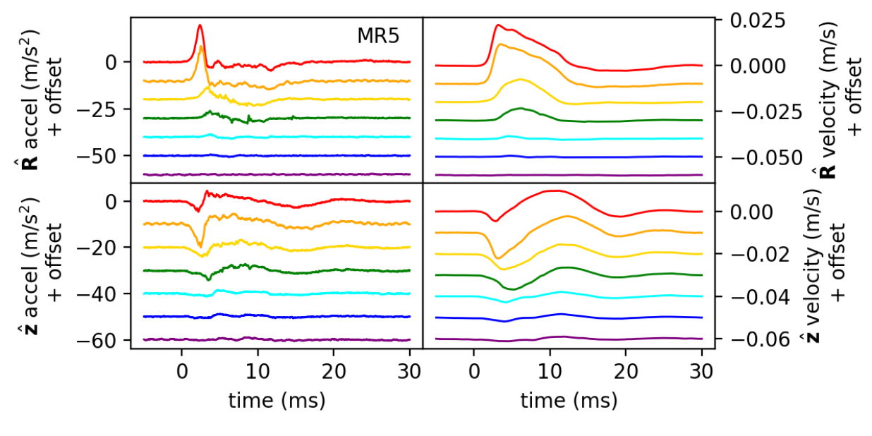
Figure 5: Similar to Figure 3 except we show the MR5 experiment data, in millet, where the accelerometers are arranged at the same cylindrical radius $R$ but at different depths.

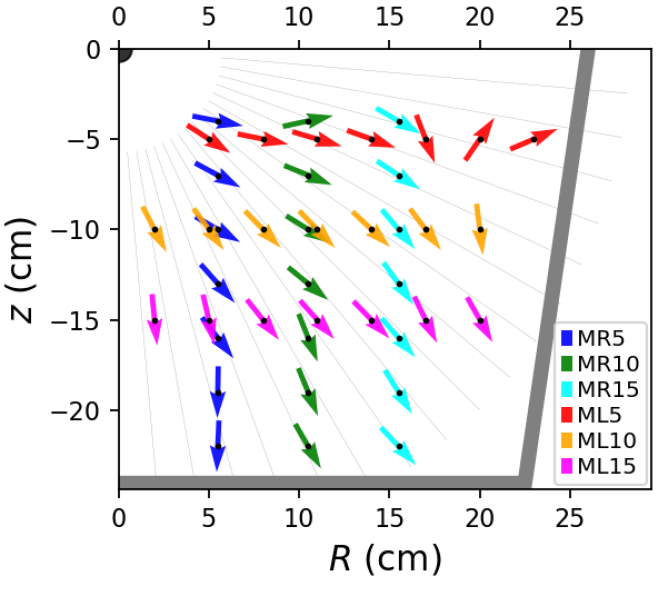
Figure 6: Ray angles are shown as colored arrows. The angles are measured from the ratio of vertical to horizontal acceleration components at the moment of peak acceleration for the ML5, ML10, ML15, MR5, MR10 and MR15 experiments in millet. Each experiment is shown with a different color arrow. Accelerometer locations are shown with black dots. Plot axes are in cylindrical coordinates, with the site of impact at the origin which is marked with a black quarter circle. The outline of the tub is shown with a thick grey line. Thin grey lines show radial rays originating from the site of impact.

3.3 Ray angles

Using the accelerometer signals and coordinates of each accelerometer, we compute the radial components of acceleration $a_{r}={\bf a}\cdot\hat{\bf r}$ and velocity $v_{r}={\bf a}\cdot\hat{\bf r}$ where unit vector $\hat{\bf r}=(R\hat{\bf R}+z\hat{\bf z})/\sqrt{R^{2}+z^{2}}$. From the radial components of acceleration, we measure the time of peak acceleration, which we denote $t_{a,prop}$ as it represents a travel or propagation time, and the value of the radial component of the acceleration at this time, $a_{r,pk}$. At the time of peak radial velocity $t_{v,prop}$ we measure the value of the peak radial velocity component $v_{r,pk}$.

In Figure 6 we show the direction of the acceleration vector $\frac{\bf a}{a}$ at the locations of each accelerometer in the millet experiments computed at the time $t_{a,prop}$. The black dots show the locations of the accelerometers and at each location a unit vector is plotted that shows the acceleration direction. The origin is the site of impact. Arrows in Figure 6 are nearly radial from the impact point. Using all the points in Figure 6, we compute the standard deviation of the acceleration angle subtracted by the angle of a ray originating from the origin and find that it is $22^{\circ}$. Discarding the 7-th and most distant accelerometer positions in each experiment, the standard deviation is $20^{\circ}$. Variations in accelerometer orientation and position and in the location of the impact can account for most of this scatter. Because the arrows in Figure 6 are nearly radial from the impact point, we infer that pulse propagation is primarily longitudinal. Large deviations are seen at large radius $R$ where the signals are weak and where reflections from the tub wall at later times could have influenced the direction of wave propagation. Since propagation rays are nearly radial, the wave propagation velocity cannot be strongly dependent upon depth. Angles computed at the time of peak velocity $t_{v,prop}$ from the velocity components are similar to those computed at peak acceleration using the acceleration components.

3.4 Peak accelerations and velocities

Because the acceleration directions imply that the pulses in our experiments are longitudinal pressure waves, we compute additional quantities using the radial ($r$) components of acceleration and velocity. In Figure 7, peak radial components of acceleration and velocity are plotted with contour plots as a function of accelerometer position. In this figure, the locations of the accelerometers are shown with black dots. The contour plots were made in python with a triangulation routine (tricontour) for irregularly sampled data. Figure 7 shows that pulse propagation is not spherically symmetric about the impact point. We estimate that peak amplitudes are about twice as large directly below the impact as at the same distance from impact but along a direction of 45^∘ from vertical.

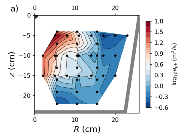
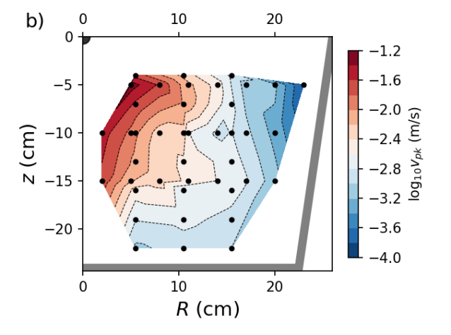
Figure 7: a) Peak pulse radial acceleration as a function of accelerometer position for the millet experiments. The thick grey line shows the outline of the tub. The black quarter circle shows the site of impact. b) Similar to a) except we plot peak radial velocity components.

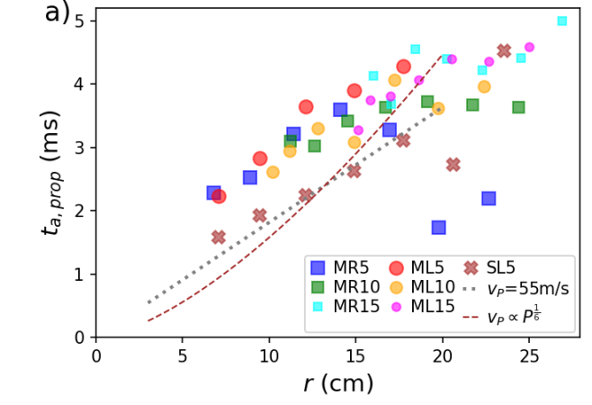
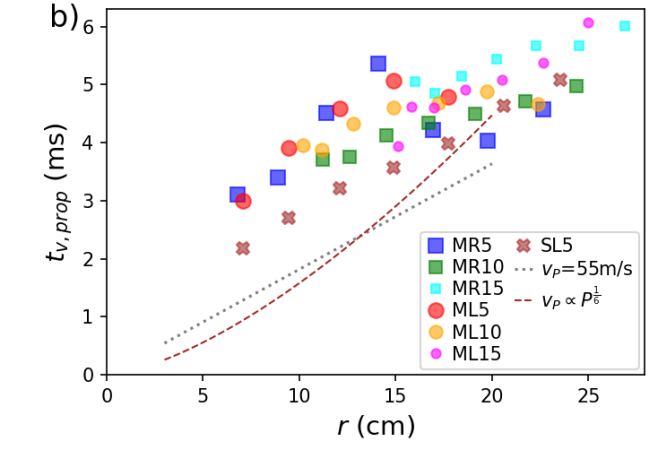
Figure 8: a) Time of peak radial acceleration $t_{a,prop}$, measured from the time of impact versus distance between impact site and accelerometer location ($r$). Each experiment comprised of 7 accelerometers is plotted with a different color marker and a point is plotted for each accelerometer in that experiment. Experiments into millet that have accelerometer positions at a single cylindrical radius $R$ are shown with square markers. Experiments into millet that have accelerometer positions at a single depth are shown with round markers. The SL5 experiment into sand is shown with brown X-shaped markers. The dotted grey line has a slope giving pulse travel speed of 55 m/s. The dashed brown line shows a model with pulse velocity sensitive to pulse amplitude. b) Similar to a) except we plot time $t_{v,prop}$ of peak radial velocity, $v_{r}$, as a function of distance from impact site.

3.5 Pulse travel speed

For the SL5 experiment into sand and the six experiments in millet (ML5, ML10, ML15, MR5, MR10, and MR15) we mark the times of the peak radial acceleration $t_{a,prop}$ in each accelerometer and plot them versus distance $r$ from the point of impact. Each experiment is plotted in Figure 8a with points that have unique color and shape. Figure 8b is similar except it shows the time of peak radial velocities, $t_{v,prop}$.

In Figure 8a and b we have also plotted a grey dotted line that corresponds to a travel velocity of $v_{P}=55$ m/s. On these plots a steeper line corresponds to a slower travel speed. The 55 m/s speed is approximately consistent with both radially and depth distributed accelerometers in millet and with the radially distributed accelerometers in fine sand. The travel speed below the surface (as measured from the MR5 experiment) is similar to that near the surface (as measured in the ML5 experiment). Surprisingly the pulse travel speed in fine sand is similar to that in millet.

A line going through the points showing millet experiments in Figure 8a, does not pass through the origin, rather it would intersect $r=0$ at about 1 ms. In Figure 8a, we plot the time of peak acceleration, not the time when the acceleration first begins to rise. The time $t=0$ is approximately the time when the projectile first touches the substrate surface. Examination of high speed video shows that the pulse is launched quite early, less than 2 ms after the projectile first touches the surface. In high speed video, motions on the surface can be seen immediately after impact with a front that moves rapidly away from the impact site before most of the ejecta curtain is launched and obscures the surface. Falling at a speed of about 5 m/s, it takes the projectile about 2 ms to drop 1 cm, a distance approximately equal to the projectile radius. The times shown in Figure 8 are those of pulse peaks, so a 1 or 2 ms delay would be consistent with the pulse peak arriving somewhat later than the rising pressure wave that is launched when the projectile first contacts the substrate surface.

Hertzian contact models predict a power-law dependence of the effective pulse travel speed $v_{P}$ on ambient or confinement pressure $P_{0}$ (Duffy and Mindlin, 1957; Liu and Nagel, 1992; Johnson et al., 2000; Somfai et al., 2005) with a scaling of $v_{P}\propto P_{0}^{\beta_{0}}$ with index $\beta_{0}\approx\frac{1}{6}$. Predictions for the index vary from 1/4 to 1/6 for models of one-dimensional (1D) chains (Herbold et al., 2009) and three-dimensional (3D) ordered (Gilles and Coste, 2003; Coste and Gilles, 2008) sphere packing. Experiments measuring a similar range in the index (Tell et al., 2020; Zhai et al., 2020). Note that $v_{P}\ll c_{g}$ where $c_{g}$ is the sound speed in the grain’s material. The travel speed of a pressure pulse may also depend on the pulse amplitude or peak pressure $P_{pk}$ with a power law scaling, $v_{P}\propto P_{pk}^{\beta_{P}}$ with index $\beta_{P}\approx 1/6$ and this is predicted theoretically and observed in experiments (Gilles and Coste, 2003; van den Wildenberg et al., 2013; Santibanez et al., 2016; Tell et al., 2020). As the pulse pressure amplitude decreases, $P_{pk}\lesssim P_{0}$, the pulse propagation speed undergoes a transition from a nonlinear and shock-like propagation regime, where the speed depends on the peak pressure, to a linear propagation regime where the propagation speed depends on the ambient or confinement pressure (van den Wildenberg et al., 2013; Santibanez et al., 2016; Tell et al., 2020). To show the possible dependence of travel speed on pressure, in Figures 8a,b we also show a dashed brown line which has pulse speed dependent on pressure in the pulse to the 1/6 power. Pulse peak pressure and pulse travel speed are estimated using equations 46 and 47 and using the model described in more detail in section 5.

There are deviations at larger distances from the impact point with pulses seen at the most distant accelerometers having shorter pulse travel times compared to those predicted by a constant speed homogeneous medium. There are also deviations at shorter distances $r<15$ cm from the impact site with longer travel times than estimated with a constant speed model.

We consider possible explanations for deviations from a linear relation between travel time and distance to the impact site.

1) Pulse travel speed could be faster with increasing depth. This would be expected if pulse travel speed is set by the strength of contacts and the contact forces depend upon hydrostatic pressure (Duffy and Mindlin, 1957; Walton, 1987; Liu and Nagel, 1992; Johnson et al., 2000). In this case we would measure a shorter travel time for distant accelerometers, compared to that predicted with a homogeneous model. Wave propagation rays would be curved. The more distant accelerometers in the ML5 and SL5 experiments would see pulses arriving from below, giving positive $z$ velocity and acceleration components.

2) The pulse travel speed depends on the pressure in the pulse itself (e.g., van den Wildenberg et al. 2013). In this case the travel speed decreases as a function of travel distance because the pulse amplitude decays as it travels. We would measure a longer travel time for more distant accelerometers, compared to that predicted with a homogeneous model. Such a model is illustrated with the brown dashed lines in Figure 8.

3) Because the pulses are broad, reflections can affect the measurement of the peak time. This primarily affects the accelerometers nearest the tub edge or bottom. If a pulse is reflected from a hard edge, a positive pressure pulse is reflected as a positive pressure pulse, but the direction of travel reverses, giving the opposite sign in acceleration and velocity and truncating the later part of the pulse. The estimated peak time of a broad pulse might be reduced by the reflected wave.

Because the time of travel decreases at larger distances, rather than increases, we infer that the mean travel speed could be faster for longer distances traveled. This is consistent with possibility 1, where the travel speed depends on depth and is faster below the surface. However, if the speeds are faster at depth, propagation rays would approach the accelerometers from below, giving a z-component in the accelerations for the most distant accelerometers and this is not seen in the MR5 or SR5 data sets and is ruled out by the acceleration directions shown in Figure 6. We discard possibility 1.

The peak pressure dependent travel speed (possibility 2) gives increasing mean travel times as a function of distance compared to a homogeneous model, where travel time is proportional to travel distance. This could be consistent with the arrival times for the accelerometers that are about 12 cm of the impact site which seem high for the MR5 and ML5 experiments, but would not be consistent with the relatively short travel times for the most distant accelerometers. Possibility 2 (pressure dependent pulse propagation velocity) could account for the relatively higher travel times at $r\sim 15$ cm but cannot account for the relatively shorter travel times at $r>15$ cm from impact site.

With a travel speed of 55 m/s it takes a wave only about 5 ms to travel from impact site on the surface horizontally to the tub edge or from impact site vertically to the tub base. Because the amplitudes drop rapidly as a function of distance from impact site, reflections would primarily affect pulse peaks seen in the accelerometers most distant from impact site. The deviations from radial acceleration directions at locations most distant from the impact site seen in Figure 6 also support this interpretation. Reflections off the tub walls (possibility 3) are the most likely explanation for the flattening of the estimated peak arrival times in the most distant accelerometers.

In summary, our pulse peak arrival times would be consistent with a pulse travel speed that is somewhat higher near the impact site than a constant velocity model due to a pressure dependence in the pulse propagation velocity. We test this possibility further by estimating the pressure in the pulses to see whether they exceed hydrostatic pressure in Section 3.6. We suspect that reflections have affected our peak time measurements for the most distant accelerometers which have the weakest and noisiest signals.

An estimate for the pulse travel speed is useful to estimate physical quantities such as the pressure amplitude of the pulse and the seismic energy efficiency. We estimate a travel speed of $v_{P}\sim 55$ m/s for both sand and millet, based on our estimate of pulse peak arrival times discussed here and we use this value in our discussions below.

Table 5: Peak values and related quantities

		MR5	ML5	SL5
Peak radial accel.	$a_{pk}$(m${}^{2}\!$/s)	17.0	51.9	43.0
Peak radial velocity	$v_{pk}$(m/s)	0.020	0.051	0.026
Adopted pulse speed	$v_{P}$ (m/s)	55		55
Speed ratio	$v_{P}/c_{g}$	$\sim\!$0.2		$\sim\!$0.03
Pressure perturbation​​​	$P_{pk}$(Pa)	840	2100	2200
Hydrostatic depth	$H_{p}$(cm)	11	28	15
Distance to impact​​​	$r$ (cm)	6.8	7.1	7.4
Distance ratio	$r/R_{cr}$	1.2	1.3	1.9
Pressure ratio	$P_{pk}/E_{g}$	8$\times\!10^{{-}6}$	2$\times\!10^{{-}5}$	2$\times\!10^{{-}7}$
Seismic Energy	$E_{seis}$(mJ)	2	9	5
Seismic efficiency	$k_{seis}$(%)	0.8	3.3	1.5

Notes: We list the peak radial velocity and peak radial acceleration in the accelerometer nearest the impact site in the MR5 and ML5 experiments into millet and in the SL5 experiment into sand. The radial distance from impact site $r$. The pressure perturbations are estimated using Equation 5 using the peak radial velocity component. Sound travel speed $c_{g}$ and elastic modulus $E_{g}$ within a grain are taken from Table 3 and used to compute the speed ratio $v_{P}/c_{g}$ and the pressure ratio $P_{pk}/E_{g}$. The depths $H_{p}$ are where peak pulse pressure would equal hydrostatic pressure and are estimated with Equation 6. The distance ratio $r/R_{cr}$ is that of the nearest accelerometer from the impact point divided by the crater radius (listed in Table 4). The seismic energy $E_{seis}$ is computed with Equation 7 and the seismic efficiency is computed with $k_{seis}=E_{seis}/K_{imp}$ and kinetic energies listed in Table 4. Both quantities are computed for the accelerometer nearest the impact site.

3.6 Estimates for the peak pulse pressure

The pressure and velocity perturbations in a sound wave are related via

$$dp\sim\rho c_{s}dv,$$ (4)

where $c_{s}$ is the sound speed and $\rho$ is the density of the medium. van den Wildenberg et al. (2013) found this relation is also obeyed for pulses propagating in a granular medium but after replacing the sound speed with an effective sound speed for pulse propagation $v_{P}$ and using density $\rho_{s}$, the bulk density of the granular medium. With the peak pressure in a pulse $P_{pk}$, and $v_{pk}$ the peak velocity, Equation 4 becomes

$$P_{pk} \sim\rho_{s}v_{P}v_{pk}.$$ (5)

Using Equation 5, we estimate the size of the pressure peaks in our pulses from the peak velocities seen in the integrated acceleration signals. We estimate the peak pressure using the velocity peak seen in the accelerometer nearest the impact site for three experiments, MR5, ML5 and SL5 with the matching substrate density for millet or sand (listed in Table 3) and our estimate for the pulse travel speed (listed in Table 5). The estimated peak pressures are about 1 kPa and are listed in Table 5.

Since hydrostatic pressure depends upon depth $H$, with $P_{0}(H)=\rho_{s}gH$ we ask, at what depth $H_{p}$ does the peak pressure match the hydrostatic pressure? The depth where peak pressure matches hydrostatic pressure, $P_{0}(H_{p})=P_{pk}$, is

$$H_{p}=\frac{P_{pk}}{\rho_{s}g_{\oplus}}.$$ (6)

These depths are also listed in Table 5 using the peak pressures measured in the accelerometers nearest impact for MR5, ML5 and SL5 experiments. The depths are 28 and 15 cm for the ML5 and SL5 experiments. Because the pulse height rapidly decreases as the pulse travels, our estimated pulse pressures exceed the hydrostatic pressure, $P_{pk}>P_{0}$ only near the impact site and near the surface. However, the distance at which the transition occurs is similar to $H_{p}$. As the depth $H_{p}$ lies within our substrate container, the transition between pulse pressure dominated and hydrostatic pressure dominated could account for variations in travel time we discussed in Section 3.5.

The ambient and hydrostatic pressure on a low-g environment such as an asteroid is low, so pulses arising from all but the lowest energy impacts would be in the non-linear pulse propagation regime (Sanchez and Scheeres, 2021). Near (within about 10 cm of) the surface and the impact site, we estimate that our experiments are just barely in a regime that might apply to low-g environments.

3.7 The pulse travel speed

We were surprised to measure similar pulse travel speeds in sand and millet. In this subsection we compare these speeds to those measured in other experiments.

Yasui et al. (2015) measured a pulse travel speed of 109 m/s in 200 $\mu$m diameter glass beads, whereas Matsue et al. (2020) measured a pulse travel speed of 53 m/s into quartz sand and similar to ours.

The wave front propagation speed within granular media is dependent on front pressure, confining or ambient pressure, and whether the substrate is organized in a lattice or is disordered (Somfai et al., 2005; van den Wildenberg et al., 2013). A polydisperse and disordered granular medium can effectively have a lower bulk modulus and so a lower pulse propagation speed compared to a similar but monodisperse medium since smaller grains do not tend to carry strong forces within the force chain network (Petit and Medina, 2018).

To compare our pulse propagation speeds to models and other experiments (as shown in Figure 8 by Somfai et al. 2005), we compute the speed ratio $v_{P}/c_{g}$ which is the pulse travel speed $v_{P}$ divided by that estimated for the grain material $c_{g}$, and we compute a pressure ratio $P_{pk}/E_{g}$ which is the peak pulse pressure $P_{pk}$ divided by the elastic modulus of the grains $E_{g}$. We use peak pressures as they are similar in size to the hydrostatic pressure in the middle of the tub. We have checked that the relation for $v_{P}/c_{g}$ vs $P_{0}/E_{g}$, using confinement pressure, measured in disordered glass spheres by Jia et al. (1999) is consistent with (to within an order of magnitude) the relation between $v_{P}/c_{g}$ and $P_{pk}/E_{g}$, using peak pressure, found by van den Wildenberg et al. (2013). Using the values for the sound speed within the grains (listed in Table 3), we estimate $v_{P}/c_{g}\sim 0.15$ in millet and 0.03 in the fine sand. Using the elastic moduli listed in Table 3 we compute $P_{pk}/E_{g}$ from the peak pressures estimated in the MR5, ML5 and SL5 experiments and list the resulting values, along with ratio $v_{P}/c_{g}$ in Table 5. The pressure ratio $P_{pk}/E_{g}\sim 10^{-5}$ in millet and $\sim 10^{-7}$ in sand.

Though we were surprised that the pulse propagation speeds are similar in sand and millet, on a plot of $v_{P}/c_{g}$ vs $P_{pk}/E_{g}$, our measurements are approximately consistent with experimental measurements in disordered glass spheres by Jia et al. (1999). Monodisperse grains in lattice structures tend to have higher propagation speeds, (as shown in Figure 8 by Somfai et al. 2005) suggesting that our low pulse propagation speeds are consistent with those predicted and measured in disordered granular media.

3.8 Seismic energy flux

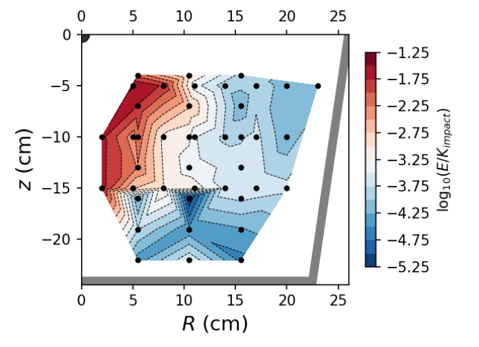
Figure 9: Similar to Figure 7 except we show the pulse seismic energy as a function of accelerometer location. Seismic energy is computed using Equation 7 using the velocity signals from each accelerometer in the six millet experiments. More energy propagates downward than horizontally.

We estimate the energy in the seismic pulse by integrating the radial velocity signal in an accelerometer $v_{r}(t)$

$$E_{seis}(r)\approx\int_{0}^{t_{1}}dt\ \rho_{s}v_{r}(t)^{2}2\pi r^{2}v_{P}$$ (7)

following Yasui et al. (2015). The radius $r$ is the distance between the impact site and the accelerometer. In Equation 7 we have assumed that the energy flux at the radius of the accelerometer is approximately $\rho_{s}v_{r}(t)^{2}v_{P}$ and equipartition between elastic and kinetic energy (supported by van den Wildenberg et al. 2013). In Equation 7, we ignore the sensitivity of pulse amplitude to angle from vertical. We integrate from $t=0$ (time of impact) to $t_{1}=10$ ms so that some energy in reflections is excluded, yet we capture most of the pulse that travels from the impact site.

The seismic efficiency $k_{seis}$ is estimated with the kinetic energy of the impact, $k_{seis}\equiv E_{seis}/K_{imp}$. Seismic energies and efficiencies are computed using Equation 7 for the MR5, ML5 and SL5 experiments for the accelerometers nearest the impact site and are listed in Table 5. These quantities are computed using our estimate for the pulse travel speed $v_{P}$, also listed in that table, the substrate densities listed in Table 3 and projectile kinetic energies that are in Table 4.

If attenuation is rapid, then an estimate for the seismic efficiency would be sensitive to distance from impact point. Our seismic efficiencies are about a percent and are larger than those computed by Yasui et al. (2015) who found $k_{seis}\sim 10^{-4}$ at a distance of $r/R_{cr}=4$ and $k_{seis}\sim 5\times 10^{-4}$ at a distance of $r/R_{cr}=1$. Here $r/R_{cr}$ is the ratio of the distance between the accelerometer and impact site and the crater radius. In comparison, our seismic efficiencies are computed for accelerometers with distance from impact $r/R_{cr}\sim 1.2$ and 2. As our impact velocities are lower than those of Yasui et al. (2015), our surprisingly large seismic efficiencies support the suggestion by Yasui et al. (2015) that seismic efficiency is sensitive to the energy of impact. At high impact energy energy is lost via shock heating and fracture. At low impact energy the fraction of energy lost could be dependent on the impact energy if attenuation is sensitive to seismic pulse pressure (van den Wildenberg et al., 2013).

In Figure 9 we plot seismic energy estimates as a function of position within the medium. For each accelerometer in the millet experiments we use Equation 7 to estimate the total seismic energy at the radius $r$ of the accelerometer. Equation 7 does not take into account the angular dependence of pulse propagation so seismic energies estimated below the surface are higher than those nearer the surface. The angular dependence resembles that of the peak velocity map shown in Figure 7b.

Table 6: Durations

		MR5, ML5	SL5
Pulse duration acc.	$\Delta t_{a}$ (ms)	1.09, 0.91	0.58
Pulse duration vel.	$\Delta t_{v}$ (ms)	4.23, 3.46	2.26
Normalized dur. acc.	$W_{a}$	0.52, 0.41	0.37
Normalized dur. vel.	$W_{v}$	1.45, 1.15	1.03
Seismic source dur.	$t_{Rss}$ (ms)	1.0	0.7

Notes: We list pulse durations $\Delta t_{a},\Delta t_{v}$ from the accelerometers nearest the impact site from the MR5 and ML5 experiments into millet and the SL5 experiment into sand. Normalized pulse durations $W_{a},W_{v}$ are the ratio of pulse width to travel time. The normalized pulse width $W_{a}$ is computed using the positive portion of the acceleration pulse and $W_{v}$ is computed using the positive portion of the velocity pulse. The crater seismic source duration $t_{Rss}$ is computed using Equation 12, the crater radii listed in Table 4 and the pulse travel speed $v_{P}$ listed in Table 5.

3.9 Pulse durations

We estimate pulse duration $\Delta t_{a}$ by measuring the FWHM (full width half max) of the first positive region in the radial component of acceleration $a_{r}$ which peaks at time $t_{a,prop}$. Similarly we measure pulse duration $\Delta t_{v}$ by measuring the FWHM of the first positive region in the radial component of velocity, $v_{r}$, which peaks at time $t_{v,prop}$. The pulse durations for the accelerometers nearest the impact site are listed in Table 6 using the MR5, ML5 experiments into millet and SL5 experiment into sand.

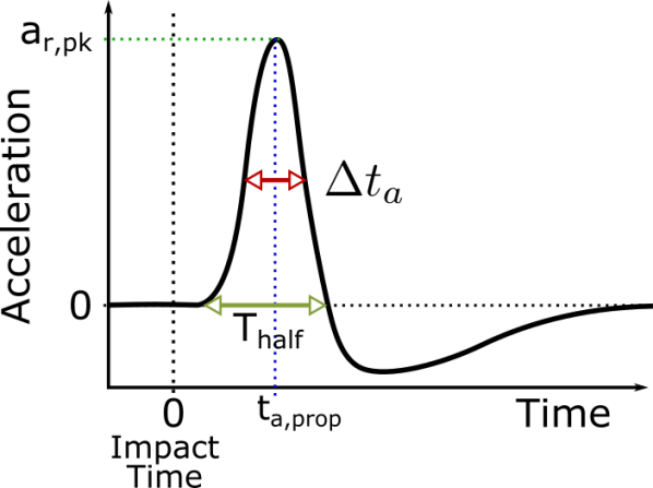
Figure 10: A schematic illustration of an impact induced pulse. We show the measured time $t_{a,prop}$ of peak acceleration $a_{r,pk}$, and the pulse duration $\Delta t_{a}$. We also show $T_{\rm half}$ used by Yasui et al. (2015) and Matsue et al. (2020) to characterize pulse duration.

A schematic of a impact induced pulse is shown in Figure 10 along with our measurements for the pulse duration $\Delta t_{a}$, time of peak $t_{a,prop}$, and peak acceleration $a_{r,pk}$. Our peak time $t_{a,prop}$ and our peak acceleration $a_{r,pk}$ correspond to $t_{max}$ and $g_{max}$, respectively, measured by Yasui et al. (2015) (see their Figure 3b) and Matsue et al. (2020) (see their Figure 6e), also in granular substrates but with higher velocity projectiles. Our measured pulse duration $\Delta t_{a}$ is about half of the duration of the positive peak, $T_{\rm half}$, measured by Yasui et al. (2015) and Matsue et al. (2020).

The positive radial acceleration pulse seen in the accelerometer nearest the impact site shown in Figure 3 has FWHM of about $\Delta t_{a}\sim 1$ ms in the ML5 experiment into millet. However, the FWHM in the similar SL5 experiment into sand has a shorter FWHM of about half the size. The duration of our acceleration pulses is similar to the parameter $T_{\rm half}\sim 0.72\pm 0.20$ ms measured by Yasui et al. (2015) for $\sim$ 100 m/s impacts into glass beads that are similar in size to our sand grains. Our pulse durations are also similar to those for 0.2 to 7 km/s velocity impacts into quartz sand measured by Matsue et al. (2020).

Yasui et al. (2015) considered three processes to account for the duration of a pressure pulse excited by an impact into a granular medium.

1) The time for a pressure wave moving at the sound speed to traverse the projectile twice $t_{D,prop}$. This time is analogous to the time for a shock to propagate forward and a rarefaction wave to propagate backward across the projectile following a high velocity impact (Melosh, 1989).

2) The time required for crater excavation.

3) A time for penetration of the projectile in the granular medium by a distance equal to the crater depth.

We compare the time for a sound wave to propagate back and forth across the projectile (listed as $t_{D,prop}$ in Table 2) to the pulse durations which are listed as $\Delta t_{a}$ in Table 4. The sound propagation times across the projectile are 0.7 and 0.01 ms for our two projectiles and are a poor match to our pulse durations. The time is shorter in the hard glass marble projectile than the softer rubber ball. Yasui et al. (2015) found that the sound crossing time was only a few microseconds for their projectiles and too small to match their pulse durations. We concur with Yasui et al. (2015) that the sound travel time across the projectile does not set the seismic pulse duration.

Using a high speed camera, Yasui et al. (2015) estimated that their craters formed in 100 to 200 ms, which exceeds their pulse widths. High speed videos of our ejecta curtains give a similar timescale. We concur with Yasui et al. (2015) that the crater excavation time does not set the seismic pulse duration.

The normal impact experiments into granular media by Goldman and Umbanhowar (2008) and Murdoch et al. (2017) have impact velocities that are similar to ours. These studies measured a stopping time, 70–200 ms, which is a time for the projectile to come to rest. With a high speed camera video taken at 1069 fps we measured that the time for the projectile to come to rest in the MR5 experiment was about $t_{stop}\sim 30$ ms. Our videos are not as sensitive to low velocities as an accelerometer embedded inside a projectile – this difference might account for the longer stopping times measured from other normal impact experiments into granular media compared to ours. Our estimated stopping time exceeds our pulse duration by an order of magnitude.

The stopping time, or time it takes the projectile to come to rest, differs from the decay time for initial deceleration which might be more relevant for seismic pulse excitation. In empirical models for projectile deceleration during a normal impact (Tsimring and Volfson 2005; Katsuragi and Durian 2007; Goldman and Umbanhowar 2008; Katsuragi and Durian 2013), the force on the projectile is the sum of a drag-like term that is proportional to the square of the projectile velocity and a depth dependent and velocity independent term. When the velocity is high, the drag-like term dominates, giving equation of motion

$$m_{p}\frac{dv_{p}}{dt}\approx-\frac{1}{2}C_{D}\rho_{s}\pi R_{p}^{2}v_{p}^{2},$$ (8)

where $v_{p}$ is the speed of the projectile and $C_{D}$ is a drag coefficient that is of order unity (Katsuragi and Durian, 2013). The regime where the velocity independent forces are neglected is called the inertial regime and the velocity squared dependence for the force in this regime is well supported by normal impact experiments into granular media (Goldman and Umbanhowar, 2008; Murdoch et al., 2017). For a spherical projectile, Equation 8 has solution for depth, speed and acceleration

$$-z_{p}(t) =\frac{1}{\alpha_{p}}\ln(v_{imp}\alpha_{p}t+1)$$

$$v_{p}(t) =\frac{v_{imp}}{v_{imp}\alpha_{p}t+1}$$

$$a_{p}(t) =\frac{v_{imp}^{2}\alpha_{p}}{(v_{imp}\alpha_{p}t+1)^{2}},$$ (9)

consistent with Equation 8 by Yasui et al. (2015). Here $v_{imp},v_{p}$ and $t$ are assumed to be positive and the inverse length-scale

$$\alpha_{p}=\frac{3C_{D}}{8R_{p}}\frac{\rho_{s}}{\rho_{p}}$$ (10)

is equivalent to the drag parameter $1/d_{1}$ by Katsuragi and Durian (2013). For our experiments with $C_{D}=1$ we find $\alpha_{p}=14,15$ m^-1 for ML5, SL5 experiments respectively. Deceleration is characterized by a time

$$t_{decel}=\frac{1}{\alpha_{p}v_{imp}},$$ (11)

which for our experiments is $t_{decel}\sim 15$ ms. This is too long to match our pulse durations $\Delta t_{v}$. Yasui et al. (2015) mitigated this problem by using the same type of empirical model but computing the time for the projectile to cross a distance equal to the crater depth, giving a time they denoted a penetration time.

As projectile stopping or deceleration times give a poor match to our pulse durations, we consider additional processes that might account for them. Impacts into granular media such as sand obey scaling laws that are independent of material strength and so are in the gravity regime (Holsapple, 1993). In the gravity regime the crater volume and radius are approximately set by scaling laws that only depend on density ratio $\pi_{4}$ and the $\pi_{2}$ parameter that is a function of the Froude number. We expect that the crater radius is set by the impactor size and speed and the substrate density. Additional properties of the medium, such as pulse propagation velocity, $v_{P}$, could influence other characteristics of the impact such as the pulse duration.

A seismic source can have a cutoff frequency in its spectrum that is set by the size of the seismic source region (Aki and Richards, 2002). A related time-scale would be the seismic source size divided by the seismic wave travel speed. For periods shorter than the seismic source time, seismic waves emitted from the near and far sides of the source would interfere, and this would give a minimum duration in a seismic pulse. The crater itself is a candidate for the size of the seismic source and this gives a crater seismic source time-scale

$$t_{Rss}=\frac{R_{cr}}{v_{P}}$$ (12)

where $v_{P}$ is the speed that the pulse travels through the medium.

Using the crater radii listed in Table 4 and the pulse travel speed (listed in Table 5 and discussed in Section 3.5), we estimate crater seismic source times of about 1.0 and 0.75 ms, respectively for the ML5 and SL5 experiments. These seismic source times are also summarized in Table 6. The crater seismic source times are similar to the duration of the pulses seen in the first accelerometer $\Delta t_{a}\approx 1.0$ and 0.5 ms, respectively for the same experiments. The crater radius in the sand experiment is smaller than those in the millet experiments, supporting the association of the $t_{Rss}$ with the seismic pulse duration.

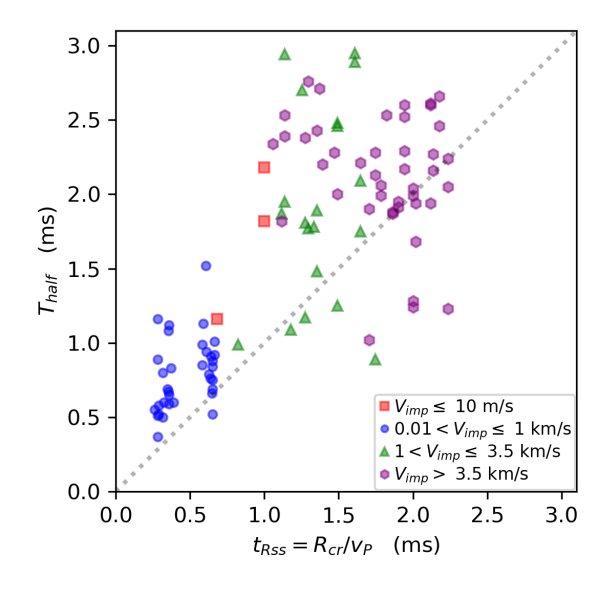
Figure 11: Pulse durations are plotted against the seismic source time. Measurements by Yasui et al. (2015) are shown with blue circles and these correspond to experiments with impact velocity about 100 m/s. Measurements by Matsue et al. (2020) are shown with blue circles, green triangles or purple hexagons, depending upon the impact velocity of the experiment. Our experiments are shown with red squares. We only plot measurements from accelerometers that are between 1 and 2.2 crater radii of the impact site.

Is the crater seismic source time similar to the pulse duration in the higher velocity impact experiments into granular media by Yasui et al. (2015) and Matsue et al. (2020)? Using the crater radii listed in Table 1 by Yasui et al. (2015) and Tables 3, 4 and 5 by Matsue et al. (2020), we estimate the seismic source times and plot them as a function of the pulse duration $T_{\rm half}$ which is the duration of the first positive portion of the acceleration pulse. The results are shown in Figure 11. The seismic source time is computed as $R_{cr}/v_{P}$ (equation 12) using the pulse travel speed $v_{P}$ measured by these experiments. For the experiments into glass beads by Yasui et al. (2015) we use pulse travel speed $v_{P}=110$ m/s, consistent with their measurement, and we use $v_{P}=50$ m/s for the into quartz sand by Matsue et al. (2020), consistent with their measurement. We also plot points for our experiments on Figure 11. We multiply our pulse durations $\Delta t_{a}$ by two, as our pulse FWHMs are about half the duration of the $T_{\rm half}$ parameter measured by Yasui et al. (2015) and Matsue et al. (2020). On Figure 11 to remove any possible sensitivity to travel distance, we only plot points from accelerometers that have distances $1<r/R_{cr}<2.2$. A dotted grey line on the figure shows $T_{\rm half}=t_{Rss}$, illustrating that to order of magnitude the two times are similar in size. In Figure 11, the different impact velocities are shown with different colored and shaped points. Figure 11 shows that over a wide range in impact velocity, pulse duration is correlated with the seismic source time. We did not exclude measurements from experiments with high density impactors, so the similarity between seismic source timescale and pulse duration holds for different density impactors. The relation is not strongly sensitive to impactor density.

Is the crater seismic source time consistent with pressure pulse duration measured for impacts into solids? The pulse widths for the impact experiments discussed by Güldermeister and Wünnemann (2017) into sandstone and quartzite have durations of about 5 $\mu$s. Their crater radii were a few cm and the pulse propagation speeds a few km/s. We find that the ratio of crater radius to pulse propagation speed is also similar in size to the pulse durations for the impact experiments by Güldermeister and Wünnemann (2017).

As the projectile penetrates the granular medium, pressure in the medium below the projectile increases. The duration of the pulse driven into the medium could be related to the mechanism for release of this pressure, in analogy to the role of the time for a shock to propagate forward and a rarefaction wave to propagate backward across the projectile following a high velocity impact (Melosh, 1989). The pressure pulse propagates through the medium at the speed $v_{P}$. The relevant distance for pressure release would be the crater radius. This gives a propagation time $R_{cr}/v_{P}$ which is equal to the crater seismic source time of Equation 12. This heuristic physical explanation for the seismic pulse duration might account for the similarity between pulse duration and the crater seismic source time-scale in our and other experiments.

Could pulse broadening of an initially narrow pulse (e.g., Hostler and Brennen 2005; Owens and Daniels 2011; Langlois and Jia 2015; Zhai et al. 2020) and associated with scattering account for our pulse durations? For pulses that are initially very short duration and propagate through a granular medium, Langlois and Jia (2015) introduced a normalized pulse duration

$$W\equiv\frac{\Delta t}{t_{prop}}$$ (13)

where $\Delta t$ is the pulse duration, as seen in pressure or velocity, and $t_{prop}$ is the pulse travel or propagation time. Because we are working with pulse velocities and accelerations, we define similar normalized pulse widths

$$W_{a}\equiv\frac{\Delta t_{a}}{t_{a,prop}},\qquad\qquad W_{v}\equiv\frac{\Delta t_{v}}{t_{v,prop}}.$$ (14)

Normalized pulse widths for the accelerometers nearest the impact site are also listed in Table 6 for the MR5, ML5 and SL5 experiments. Langlois and Jia (2015) found that the normalized pulse width

$$W\approx C_{W}\sqrt{\frac{d_{g}}{r}}$$ (15)

where $d_{g}$ is the grain diameter, $r$ is the travel distance and dimensionless coefficient $C_{W}\sim 1$.

Using a mean grain diameter of 3 mm for millet and 0.3 mm for the fine sand we estimate $\sqrt{d_{g}/r}\sim 0.2$ for the first accelerometer in the ML5 experiment and $\sqrt{d_{g}/r}\sim 0.06$ for the first accelerometer in the SL5 experiment. However, normalized pulse widths in velocity are $W_{v}\sim 1$. Only if the coefficient $C_{W}$ is 5 to 20 and significantly greater than 1 could the diffusive model by Langlois and Jia (2015) match the normalized velocity pulse widths, assuming that pulse widths were initially shorter than a ms. The rate of pulse broadening could be sensitive to pulse peak pressure, as suggested by the pulse pressure dependent attenuation rate seen in experiments of strong pulses (van den Wildenberg et al., 2013), so a higher effective value of $C_{W}$ is possible.

In summary, a time based on the size of the crater and the speed that pulses travel through the granular medium is a possible time-scale that could account for the duration of the pulses we see in our experiments and in higher velocity experiments. The shorter duration pulses in sand suggest that pulse duration could also be sensitive to grain size, as suggested by models of pulse broadening Langlois and Jia (2015). Our pulse durations could be consistent with an initially short duration pulse (less than 1 ms) and subsequent broadening described by Equation 15, but only if the scaling coefficient $C_{W}$ is about 10 and an order of magnitude larger than measured by Langlois and Jia (2015).

3.10 Pulse broadening

To best study variations in pulse shape, we look at the strongest signals which are those nearest the site of impact. We focus on the radial accelerations and velocity from the four accelerometers nearest the site of impact in the ML5 experiment into millet and the SL5 experiment into sand. These two experiments have the same coordinate positions for the accelerometers and their signals were previously shown in Figures 3 and 4. In Figure 12 we show radial acceleration and velocity signals normalized so that the peaks have the same height. Figure 13 is similar but the signals have been shifted in time so that the peaks are near a time of zero. Figure 12 and 13 shows that the pulses are broader in millet than in sand and that the pulses broaden and become smoother as they travel through the granular medium.

In Figure 14 we show power spectra of the acceleration signals shown in Figure 12 as a function of frequency. The signals are multiplied by a Hanning window function and the mean subtracted prior to computing the Fourier transform. We use a window that is 12 ms long for the accelerations and 35 ms long for the velocities. The power spectra have been normalized so that their peak is 1. The spectrum has zero power at zero frequency because the mean signal value was subtracted. Figure 14a shows that the accelerometers nearest the site of impact peak have more power at higher frequencies than those more distant from the site of impact.

Pulse broadening is most clearly seen in the sand experiment (see bottom panels of Figures 12a, and 13) in part because the pulse is initially shorter. However, smoothing of the pulse shape is most clearly seen early, where the pulse accelerations and velocities rise in both sand and millet experiments (see Figures 12a,b). If attenuation is dependent upon frequency, pulses would become smoother as they travel. This is consistent with the power spectra we show in Figure 14 that show that the pulses preferentially lose power at higher frequencies as they travel. We attribute steep slopes where velocities drop in the accelerometers most distant from thee impact site to a reflection from the tub rim.

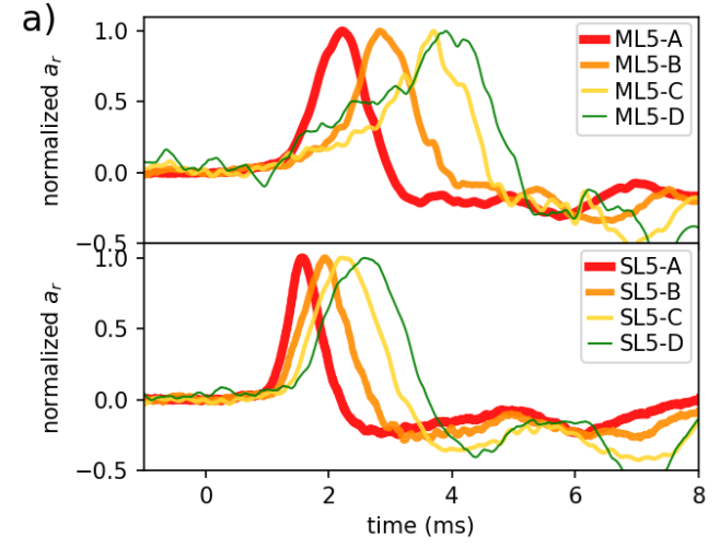
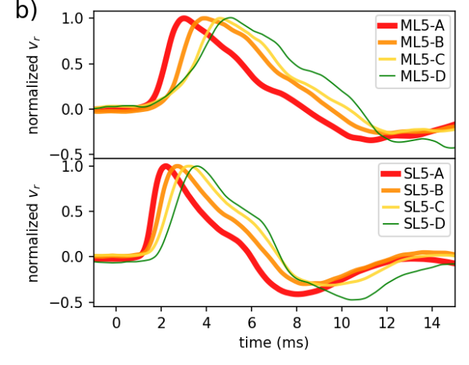
Figure 12: a) The radial component of acceleration is shown as a function of time for the four accelerometers nearest the impact site from the ML5 experiment into millet in the top panel and in the SL5 experiment into sand in the bottom panel. Here A, B, C, D refer to the accelerometers in order of distance from the site of impact. The signals have been scaled so that they have the same peak heights. Pulses broaden and become smoother as they travel, and the pulses in the millet experiment are broader than those in the sand experiment. Smoothing is particularly noticeable on the rising side of the pulses. b) Similar to a) except we show velocities.

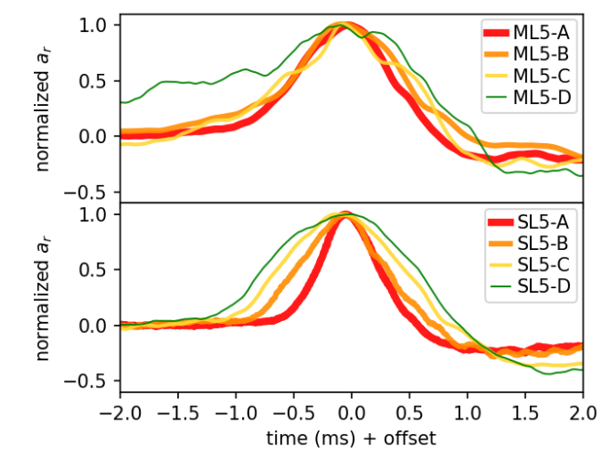
Figure 13: Similar to Figure 12a showing accelerations except times have been shifted so that the peaks occur at a time of about zero.

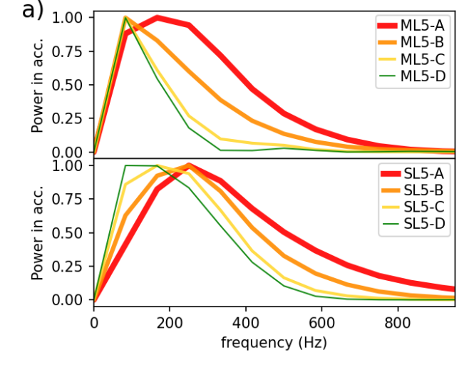
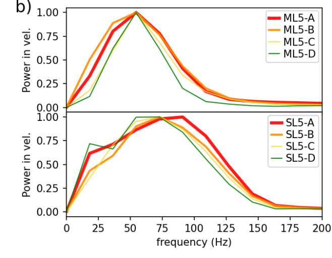
Figure 14: a) Power spectra of the acceleration pulses from the four accelerometers nearest the point of impact from the ML5 (top panel) and SL5 experiments (bottom panel). b) Similar to a) except showing power spectra of the velocity pulses.

We discuss the pulse duration regime for our experiments. Our pulse durations are about a ms and correspond to a spatial width $\sim$ 50 mm (estimated using $v_{P}$), and this corresponds to a wavelength of about $\lambda\sim 100$ mm. Our grains have diameters of 3 and 0.3 mm respectively for millet and sand, respectively. This gives ratio of wavelength to grain diameter $\lambda/d\sim 30$ and 300 for the millet and sand experiments, respectively. The experiments by Langlois and Jia (2015) in glass beads had grain diameters ranging from 0.22 to 5 mm and the pulse travel speed was 800 m/s. Their pulse durations ranged from about 5 to 42 $\mu s$ (following their Figure 5a) giving spatial pulse widths of 4 to 34 mm, corresponding to wavelengths of $\lambda\sim$ 8 to 70 mm. This would give $\lambda/d$ ranging from about 2 to 300. Because pulse durations were in the regime $\lambda/d>1$, Langlois and Jia (2015) proposed that the attenuation was due to scattering caused by variations in grain stiffness, rather than due to variations in travel times along different force contact chains (Owens and Daniels, 2011). Hostler and Brennen (2005) measured pulse broadening in a regime where pulse width was about $10^{3}$ times the pulse travel time across a single grain giving $\lambda/d\sim 10^{3}$. Thus at least three sets of experiments have measured pulse broadening in the regime $\lambda/d>1$.

The scaling observed by between pulse width and travel distance by Langlois and Jia (2015) obeyed scaling that they interpreted as due to attenuation rather than dispersion. Broadening and smoothing of the pulse shape is likely to be connected to dissipation mechanisms. In contrast, a dispersive mechanism need not be associated with dissipation. Energy can be dissipated via several mechanisms which can operate at $\lambda/d>1$, including frictional and inelastic particle interactions (discussed by Hostler and Brennen 2005), particle rearrangements (discussed by Zhai et al. 2020), scattering through the particle contact network (Owens and Daniels, 2011) and scattering due to variations in particle stiffness (Langlois and Jia, 2015), variations in the packing fraction or porosity and variations in the connectivity of the particle contact network.

4 Pulse smoothing and attenuation

Figures 3, 4, 5, 12, 13 and 14 illustrate that the pulses in our experiments broaden and become smoother as they travel through the granular medium. The pulses do not break up into a series of high frequency waves followed by low frequency ones, or vice versa, as would be expected for dispersive model for wave propagation. We primarily observe attenuation, smoothing and broadening, which are characteristics of diffusion and not of dispersion.

Granular systems can display both solid-like and fluid-like behavior (e.g., GDR-MiDi 2004; Forterre and Pouliquen 2008). We introduce both elastic and hydrodynamic continuum models for wave propagation. For propagation of elastic waves in one dimension in an isotropic medium, momentum conservation can be written as

$$\rho\frac{\partial u}{\partial t}=-\frac{\partial\sigma}{\partial x}$$ (16)

where the velocity field $u(x,t)=\frac{\partial\delta}{\partial t}$, with $\delta(x,t)$ the displacement field, and $\sigma$ is one component of the stress tensor. With stress linearly proportional to the strain (which depends on the gradient of the displacement field) and in the low amplitude limit, a wave equation for propagation of longitudinal waves is derived

$$\frac{\partial^{2}\delta}{\partial t^{2}}=v_{P}^{2}\frac{\partial^{2}\delta}{\partial x^{2}},$$ (17)

(e.g., Aki and Richards 2002, section 2). This gives a dispersion relation $\omega^{2}=v_{P}^{2}k^{2}$ where $\omega$ is the angular frequency of a traveling sine wave that has wave number $k$. A more general model for the dispersion relation would give a complex and non-linear function that is non-linear. If $\omega(k)$ or $k(\omega)$ has a complex component, this can be interpreted in terms of a wavelength or frequency dependent decay rate for the amplitude. This is commonly described as attenuation. If $\omega(k)$ is real but non-linear then the system is described as dispersive. Dispersion naturally arises if the Taylor expansion of the elastic stress depends on the second or higher order spatial derivatives of the displacement field. In this case the model is said to be ‘anelastic’.

If dispersion and attenuation are low and pulses propagate in one direction to positive $x$ then equation 17 is consistent with $\frac{\partial u}{\partial t}+v_{P}\frac{\partial u}{\partial x}=0$ which is known as the advection equation. The same relation can be derived for hydrodynamics in the low amplitude limit using Euler’s equation, conservation of mass and an equation of state, with $v_{P}$ equivalent to the velocity of sound. Conservation of mass to first order in perturbation amplitudes, the equation of state and a nearly wavelike solution gives $\frac{1}{\rho}\frac{dp}{dx}\approx v_{P}\frac{du}{dx}$ where $p$ is pressure. Neglecting the non-linear inertial term, the Navier Stokes equation becomes

$$\frac{\partial u}{\partial t}=-v_{P}\frac{\partial u}{\partial x}+D\frac{\partial^{2}u}{\partial x^{2}}.$$ (18)

Here $D=\nu/v_{P}$ depends on the kinematic viscosity $\nu$. The Navier Stokes equation is also derived via momentum conservation with stress tensor dependent upon pressure, ram pressure, viscosity and the velocity gradient. Equation 18 is an advection-diffusion equation. The integral $\int u(x,t)dx$ is a conserved quantity, so density variations need not be taken into account to maintain conservation of momentum. A solution to equation 18 that is initially a delta function is

$$u(x,t)=\frac{1}{\sqrt{4Dt}}e^{-\frac{(x-v_{P}t)^{2}}{4Dt}}.$$ (19)

The dispersion relation for equation 18 is $\omega=v_{P}k+iDk^{2}$ and the viscous or diffusive behavior causes attenuation.

Granular flows often exhibit a dependence on the shear rate, which gives them a viscous-like behavior (Forterre and Pouliquen, 2008). Viscous or diffusive behavior in the context of elastic waves arises naturally if the stress tensor is dependent on the strain rate, which depends on the time derivative of the displacement field. The stress can gain a term dependent on $\frac{\partial^{2}\delta}{\partial x\partial t}$, giving an additional term $\propto\frac{\partial^{3}\delta}{\partial x^{2}\partial t}=\frac{\partial^{2}u}{\partial x^{2}}$ in the wave equation (equation 17), which resembles the diffusive term in equation 18. In this case, the model is said to be ‘visco-elastic’.

Because equation 18 contains a diffusion term, short wavelength structure attenuates more quickly than those at longer wavelengths. A velocity pulse will become smoother as it travels and an initially narrow pulse will broaden. The association of equation 18 with conservation of momentum motivates using the velocity field as a key variable.

Because our experiments primarily show attenuation and smoothing, rather than dispersive behavior, we adopt a diffusive model, with velocity as key variable to model the propagation of our pulses. Our experiments predominantly show a single pulse that rapidly attenuates as it travels, confirming results from prior experiments of impacts into granular media (McGarr et al., 1969; Yasui et al., 2015; Matsue et al., 2020). This motivates describing the pulse with two parameters: an amplitude and a duration. An advantage of an advection-diffusion model for pulse propagation into a half sphere is that the rate that the pulse duration grows is directly related to the pulse amplitude decay rate. This gives a simple model that predicts how pulse amplitude, pulse width and energy vary with propagation distance. We can compare the resulting scaling relations to the dependence of pulse width and peak amplitudes on distance from impact site in our experiments.

We first show that the model for pulse broadening proposed by Langlois and Jia (2015) is consistent with an advective-diffusion model for velocity propagation. We do this showing that their scaling law (Equation 15), relating pulse width to travel distance, can be derived via a diffusive model characterized with a diffusion coefficient $D$. The propagation distance $r$ is related to the pulse travel time via $r=v_{P}t_{prop}$ where $v_{P}$ is the pulse travel speed. We define $\Delta r=\Delta tv_{P}$ as the spatial pulse width. Diffusive broadening of a delta function at $t=0$ (as in equation 19) gives pulse width $\Delta r\sim\sqrt{Dt_{prop}}$ as a function of propagation time $t_{prop}$. This spatial width corresponds to a pulse duration

$$\Delta t\approx\frac{\sqrt{Dt_{prop}}}{v_{P}}\approx\sqrt{Dr/v_{P}^{3}}.$$ (20)

Using Equations 13 and 20, the normalized pulse duration

$$W\sim\sqrt{\frac{D}{rv_{P}}}.$$ (21)

Comparison of this equation with the scaling relation by Langlois and Jia (2015) in Equation 15 implies that this relation is consistent with diffusion coefficient that depends on pulse propagation speed and grain size

$$D\sim C_{W}^{2}d_{g}v_{P}.$$ (22)

We have illustrated that the scaling relation (Equation 15) by Langlois and Jia (2015) can be derived via a diffusive model for pulse propagation of an initially narrow pulse and with diffusion coefficient given by Equation 22. Tell et al. (2020) also adopted a diffusive model for scattering and their experiments were also consistent with a diffusion coefficient in the form of Equation 22 with $C_{W}\sim 1$ (see their Section VI).

If the pulse is not initially a delta function then diffusive broadening gives a pulse duration $\Delta t\approx\sqrt{\Delta t_{0}^{2}+Dr/v_{P}^{3}}$ where $\Delta t_{0}^{2}$ is the duration at $t=0$ and at $r=0$. Instead of writing pulse duration in terms of that at $t=0$ we scale from the pulse duration for the pulse at a distance of the crater radius. The pulse duration for $r>R_{cr}$

$$\Delta t(r)\approx\sqrt{\frac{D(r-R_{cr})}{v_{P}^{3}}+\Delta t_{Rc}^{2}},$$ (23)

where $\Delta t_{Rc}$ is pulse width at $r=R_{cr}$.

In Figure 15a we plot pulse duration $\Delta t_{v}$ (the full width half max of the first positive portion of the radial velocity pulse) for the MR5, ML5, ML10, SL5 and SL10 experiments. On this plot, the dashed brown and dotted orange lines show pulse durations estimated with Equation 23 and with diffusion coefficient $D$ and duration $\Delta t_{Rc}$ listed in the key. The orange dotted line uses $R_{cr}$ for the millet experiments and the brown dashed lines uses $R_{cr}$ for the sand experiment. Using Equation 22 and a mean size for the millet grains ($d_{g}=3$ mm), the diffusion coefficient for the dotted orange line is consistent with scaling coefficient $C_{W}=12$. Using the mean sand grain size (0.3 mm), the dashed brown line gives $C_{W}=30$, The diffusion coefficient is lower in the sand, as would be expected if the broadening rate were sensitive to grain size. However, the mean sand grain size is about an order of magnitude smaller than the size of the millet grains and Equation 22 predicts $D\propto d_{g}$. The $C_{W}$ values are about an order of magnitude larger than expected (in comparison to experimental measurements by Langlois and Jia 2015; Tell et al. 2020), as we previously estimated in Section 3.9. The initial durations we use for the dotted orange and dashed brown lines have $\Delta t_{Rc}$ at $r=R_{Cr}$ that are 3 times and 1.5 times $R_{cr}/v_{P}$ for the millet and sand experiments, respectively. As discussed in Section 3.9, these initial durations are similar to the seismic source times. Figure 15b is similar to Figure 15a except we show $\Delta t_{a}$ instead of $\Delta t_{v}$. Pulse broadening is also seen Figure 15b.

Figure 15 shows that pulses initially broaden with an estimated diffusion coefficient that exceeds that which we would have estimated using relations by Langlois and Jia (2015); Tell et al. (2020), with $C_{W}\sim 1$, by about an order of magnitude. Past about 15 cm from the impact site, pulses are weaker and the widths could be affected by reflections, so we are not concerned by the low durations measured from the accelerometers more distant from the impact site.

The curves on Figure 15 illustrate that the diffusion coefficient is sufficiently large that even a few crater radii away from impact, the diffusion term in Equation 23 dominates the pulse duration and the initial pulse duration is less relevant. In other words, Equation 23 can be approximated by Equation 20. The simpler power-law form of Equation 20 facilitates predicting attenuation, so we will use it in the following sections.

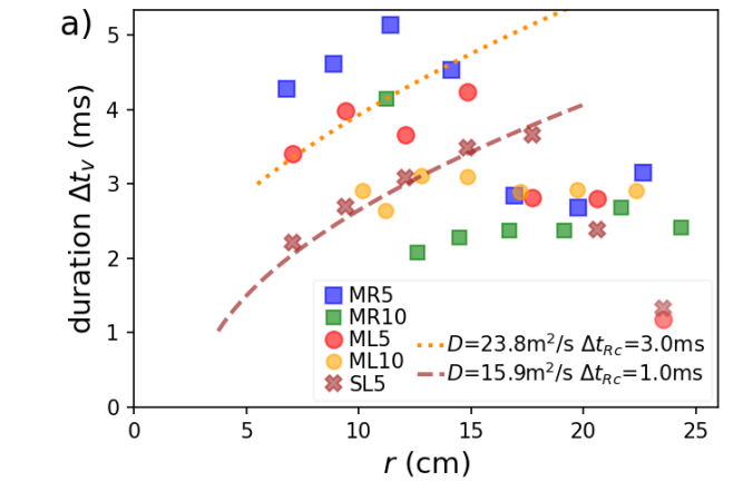
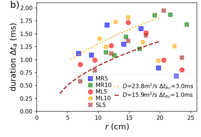
Figure 15: a) Pulse duration, the FWHM, $\Delta t_{v}$, in ms as a function of travel distance for the MR5, ML5, ML10, MR10 and SL5 experiments. Brown dashed and orange dotted lines are computed using Equation 23, diffusion coefficients $D$ and duration $\Delta t_{Rc}$ at $r=R_{cr}$ listed in the key. b) Similar to a) except showing $\Delta t_{a}$.

4.1 Pulse amplitudes

With pulse broadening due to diffusion of a pulse’s velocity, what attenuation is implied? We consider a pulse that propagates radially into a half sphere with peak amplitude in velocity $v_{pk}(r)$ which is a function of propagation distance. If the pulse propagates radially from the origin and isotropically, then momentum conservation implies that

$$\rho_{s}v_{pk}(r)\Delta t_{v}v_{P}2\pi r^{2}={\rm constant}.$$ (24)

This follows by integrating the momentum flux as a function of time in a pulse that passes radius $r$ and in a small region of solid angle. Here $\Delta t_{v}$ is the width of the velocity or pressure pulse. In Equation 24 we neglect the angular dependence of pulse amplitude, however this equation could be modified to depend on the spherical coordinate polar angle from the surface normal. Equation 24 and using Equation 20 for $\Delta t_{v}$ implies that the peak velocity

$$v_{pk}(r)\propto r^{-\frac{5}{2}}v_{P}^{\frac{1}{2}}D^{-\frac{1}{2}}.$$ (25)

What do we expect for the radial scaling of the magnitude of the peak acceleration? The peak acceleration $a_{pk}\sim\frac{v_{pk}}{\Delta t_{v}}$. Using Equation 25 for the peak velocity and Equation 20 for $\Delta t_{v}$

$$a_{pk}(r) \propto r^{-3}v_{P}^{2}D^{-1}.$$ (26)

The peak particle displacement in the pressure pulse we estimate from Equations 25 and 20

$$\delta_{pk}(r)\sim v_{pk}\Delta t_{v}\propto r^{-2}v_{P}^{-1}.$$ (27)

Above we have estimated the radial scaling of peak acceleration and velocity. We now use the momentum of the projectile to estimate the constants of proportionality for Equations 25 and 26. Using Equation 9, the projectile deceleration at the moment of impact is

$$a_{p,max}\approx-\alpha_{p}v_{imp}^{2}.$$ (28)

If the projectile deceleration is due to the launch of a pressure pulse within the medium, then momentum conservation can be used to estimate the size of the pressure pulse. At the crater radius we assume that

$$b_{\rm eff}m_{p}\frac{dv_{p}}{dt}\sim\rho_{s}\pi R_{cr}^{2}v_{pk}(R_{cr})v_{P}$$ (29)

where on the right side the momentum flux from a pulse that travels from the projectile surface with velocity $v_{P}$ and with a peak radial velocity perturbation $v_{pk}(R_{cr})$ at distance $r=R_{cr}$ from the impact site is matched to the deceleration of the projectile which is on the left. We include a dimensionless factor $b_{\rm eff}$, similar to the factor known as the momentum transfer efficiency or $\beta$ parameter (Housen and Holsapple, 2011; Holsapple and Housen, 2012; Jutzi and Michel, 2014), which is the total momentum change of an asteroid resulting from an impact, divided by the projectile momentum. Our momentum transfer efficiency $b_{\rm eff}$ is not the same as that commonly used to compute the momentum transfer efficiency resulting from an asteroid impact as all the ejecta in our experiments returns to hit the surface, and none of it escapes into space. Also, the projectile’s momentum is a vector but in the right hand side of Equation 29 we integrate the flux of the radial momentum component in the seismic pulse over a hemisphere. Our dimensionless momentum transfer efficiency includes an integration factor that relates two similar sized quantities with units of momentum.

Equation 29, using the maximum projectile deceleration in Equation 28 for $dv_{p}/dt$ and Equation 10 for $\alpha_{p}$, we estimate the peak pulse velocity at $r=R_{cr}$,

$$v_{pk}(R_{cr})\sim\frac{b_{\rm eff}C_{D}}{2}\frac{R_{p}^{2}}{R_{cr}^{2}}\frac{v_{imp}^{2}}{v_{P}}.$$ (30)

Using our impact velocities, $b_{\rm eff}C_{D}=1$, crater sizes listed in Table 4, the pulse propagation speed listed in Table 5 and projectile radii listed in Table 2, we estimate that $v_{pk}(R_{p})\sim 0.02$ m/s for the millet experiments and 0.03 m/s for the sand experiment. These values are similar to those listed in Table 5 for the accelerometers nearest the impact site and with $r/R_{cr}\sim 1.2$ and 2 for the millet and sand experiments, respectively.

We use the peak velocity at $r=R_{cr}$ (Equation 30) to determine the constant of proportionality in Equation 25,

$$v_{pk}(r)\approx v_{pk}(R_{cr})\left(\frac{r}{R_{cr}}\right)^{-\frac{5}{2}}.$$ (31)

An estimate for the peak acceleration at $r=R_{cr}$, given by $a_{pk}\approx v_{pk}/\Delta t_{v}$, depends on the pulse duration at the crater radius or at $r=R_{cr}$. We can estimate the pulse duration $\Delta t_{v}$ with Equation 20 or from the time it takes a pressure wave to traverse the crater radius. As we discussed in Section 3.9, the diffusion based estimate required a large $C_{W}$ scaling coefficient but both estimates gave potential matches to the pulse duration at $R_{cr}$. The pulses in our experiments broaden as they travel, as shown in Figures 13. We opt to use the crater radius to estimate normalization factors that depend on $\Delta t_{v}$, giving

$$\Delta t_{v}(R_{c})=\frac{R_{cr}}{v_{P}},$$ (32)

but we adopt scaling derived from the diffusive model to predict how the amplitudes drop with distance from the site of impact.

Using the time it takes the pulse to cross the crater radius for the pulse duration $\Delta t_{v}$ at $r=R_{cr}$ (equation 32), we estimate the peak acceleration

$$a_{pk}(R_{cr})\approx\frac{v_{pk}(R_{cr})v_{P}}{R_{cr}}.$$ (33)

Using this as the constant of proportionality for Equation 26 the peak acceleration

$$a_{pk}(r)\approx a_{pk}(R_{cr})\left(\frac{r}{R_{cr}}\right)^{-3}.$$ (34)

Likewise the peak displacement at $r=R_{cr}$

$$\delta_{pk}(R_{cr})\approx\frac{v_{pk}(R_{cr})R_{cr}}{v_{P}}.$$ (35)

The exponent of -3 for the decay of the peak acceleration is nearly consistent with the value of $3.18\pm 0.10$ measured for peak accelerations in high velocity impact experiments into quartz sand (Matsue et al., 2020).

In Figure 16 we plot peak velocities and peak accelerations as a function of distance $r$ from impact site for all accelerometers in the six millet and single sand impact experiments. The dotted orange and dashed brown lines shows the prediction for how the peak acceleration and velocity would drop with radius derived via this simple diffusive attenuation model (computed using Equations 25, 26, 30 – 34). The dotted orange lines use impact velocity, projectile and crater radius for the millet experiments and the dashed brown lines use the same quantities but for the sand experiment. We have adjusted the produce of the momentum transfer efficiency parameter and drag coefficient $b_{\rm eff}C_{D}$ so that the lines are consistent with the accelerometers nearest the site of impact. Our simple diffusion model provides a decent match to the decay rates for the peak velocities and accelerations in our accelerometers, particularly at positions nearest the site of impact where reflections don’t affect the signal and the signals are stronger. To match the pulse amplitudes we require a momentum transfer efficiency parameter $b_{\rm eff}C_{D}\sim 4$ or 7, for the millet and sand experiments, respectively. We would expect this parameter to be greater than 1 as the seismic pulse must balance the momentum required to both stop the projectile and launch the ejecta curtain and the drag coefficient could exceed 1.

The power law index of -2.5 predicted for decay of the peak velocity (Equation 25) with our simple diffusion model into a granular medium is steeper than the value of -1 measured for the decay exponent for pressure amplitude of sandstone in the elastic regime (Güldermeister and Wünnemann, 2017). An exponent of -1 in the pressure amplitude implies that there is little energy lost as the pulse travels. With a constant $v_{P}$, Equation 5 implies that when there is little attenuation, the peak velocity $v_{pk}\propto r^{-1}$ would have a similar exponent. In Figure 16 we plot a dot-dashed black line that has $v_{pk}\propto r^{-1}$. Pulses in our experiments decay much more rapidly than shown with this black line. The -1 exponent for $v_{pk}$ is ruled out by our experiments.

With higher velocity impacts (about 100 m/s) into glass beads Yasui et al. (2015) measured an attenuation relation between peak acceleration and distance to impact $a_{pk}\propto r^{-2.21\pm 0.12}$ (their equation 6). With impact velocities of 1 to 7 km/s into quartz sand Matsue et al. (2020) measured a similar exponent; $a_{pk}\propto r^{-3.18\pm 0.10}$. In Figure 16b we also plot two lines with these measured indices. The decay of peak acceleration we see in our experiments and predicted with our model is consistent with the power-law indices measured by these higher velocity impact experiments.

In the diffusive model, because the pulse broadens, the velocity amplitude decreases even while conserving momentum (assumed in Equation 24). This simple model directly relates pulse broadening to energy decay. A lossy collisional model gives an analogy. Each collision redistributes momentum to additional particles, reducing the mean value in a pulse. Eventually all particles have the same velocity. The energy decreases, while the distribution of momentum broadens.

Equations 25 and 31 neglect the dependence of pulse amplitude on polar angle. We can compare the slope of the points in different experiments in Figure 16. The decay rate of the peak velocity $v_{pk}$ in the ML5 experiment is faster than that of the MR5 experiment. This difference in decay rates can be attributed to the angular dependence of the peak velocity. At the same distance from the site of impact, the MR5 experiment has deeper accelerometers than the ML5 experiment and these deeper accelerometers see higher pulse amplitudes.

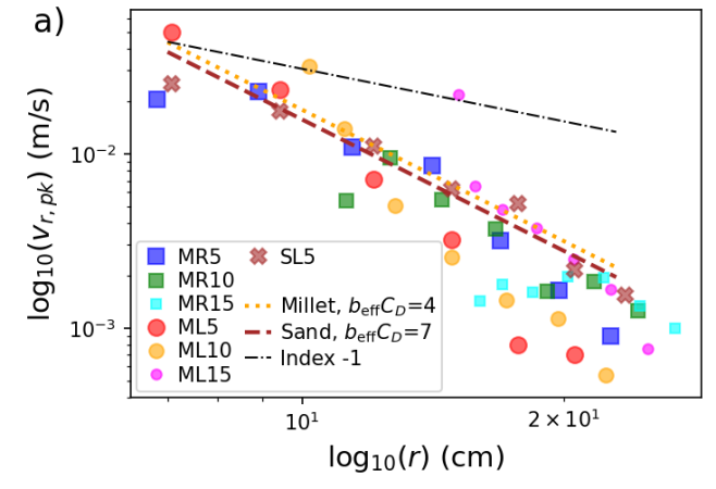
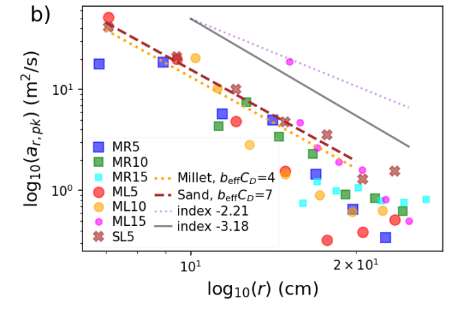
Figure 16: a) Peak pulse velocity as a function of travel distance for the 6 millet and single sand experiments. The point types are the same as shown in Figure 8. Each point is from a single accelerometer. The dotted orange line and dashed brown lines are computed using Equation 31 with constant of proportionality from Equation 30. The power law index is predicted via Equation 25 using a diffusive attenuation model for pulse propagation. The dotted orange line uses parameters for the millet experiments and the dashed brown line used parameters for sand experiment. The product of the momentum transfer efficiency parameter and the drag coefficient $b_{\rm eff}C_{D}$ has been adjusted to be consistent with points nearest impact and with values are given in the key. The dot-dashed black line shows a model with $v_{pk}\propto r^{-1}$ corresponding to little attenuation. The peak velocities are poorly described by the black line, so attenuation is rapid. b) Peak accelerations as a function of travel distance. The dotted orange line and dashed brown lines are similarly computed using Equation 34 with constant of proportionality from Equation 33. The thin solid pink line shows $a_{r,pk}\propto r^{-2.21}$ using the index measured by Yasui et al. (2015). The thin solid grey line shows $a_{r,pk}\propto r^{-3.18}$ measured by Matsue et al. (2020).

4.2 Seismic energy decay

We estimate how our estimate for the total seismic energy that passes radius $r$ would scale with radius using the diffusive model discussed above in Section 4.1. The seismic energy can be estimated by integrating the energy flux as a function of time of a pulse that passes radius $r$, giving

$$E_{seis}(r)\sim\rho_{s}v_{pk}^{2}(r)\Delta t_{v}v_{P}2\pi r^{2},$$ (36)

consistent with Equation 7. Using Equation 25 for $v_{pk}$ and Equation 20 for $\Delta t_{v}$ we find that

$$E_{seis}(r) \propto r^{-\frac{5}{2}}v_{P}^{-\frac{1}{2}}D^{-\frac{1}{2}}.$$ (37)

As done in Section 4.1, we estimate the constant of proportionality by substituting Equation 30 for $v_{pk}(R_{cr})$ and with $\Delta t_{v}(R_{cr})=R_{cr}/v_{P}$, at crater radius $r=R_{cr}$,

$$E_{seis}(R_{cr}) \approx\rho_{s}\left[\frac{b_{\rm eff}C_{D}}{2}\frac{R_{p}^{2}}{R_{cr}^{2}}\frac{v_{imp}^{2}}{v_{P}}\right]^{2}2\pi R_{cr}^{3}.$$ (38)

In Figure 17 we show seismic energy estimated from each accelerometer using Equation 7 as a function of distance $r$ from impact site along with a dotted grey line that shows the $r^{-\frac{5}{2}}$ scaling predicted via Equation 37, and with constant of proportionality from Equation 38. We use the same momentum transfer efficiencies as in Figures 16. At small radius $r$ from the impact site, the estimated seismic energies exceed the predicted estimate because the seismic energies take into a longer time interval than only the first positive portion in velocity. As was true for the peak accelerations and velocities, the estimated decay rate is a reasonable match to the measurements from accelerometers nearer the impact site. Also as was true for peak accelerations and velocities, many points lie below the predicted line at larger distances. This discrepancy can in part be attributed to loss of energy through the tub base into the floor.

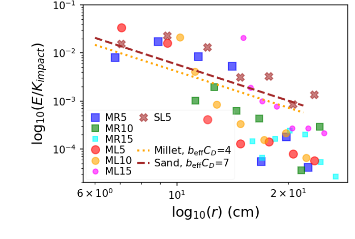
Figure 17: Seismic energy in the pulse as a function of the distance of each accelerometer from the site of impact. Total seismic energy is computed for each accelerometer using Equation 7 and is in units of the kinetic energy of impact. The point types are the same as shown in Figure 8. The dotted orange and dashed lines show the power law function $E_{pk}\propto r^{-\frac{5}{2}}$ predicted via Equation 37 and with constant of proportionality from Equation 38, computed using parameters for the millet and sand experiments, respectively. The key shows the assumed momentum transfer efficiency parameters for these two lines.

4.3 Extension to higher velocity impacts

Our power law scaling relations for physical properties have constant of proportionality based on physical quantities at the crater radius $R_{cr}$. However, in section 4.1 we based our estimate for the peak velocity at $R_{cr}$ (equation 30) on the product of a drag coefficient, $C_{D}$, and a momentum transfer parameter $b_{\rm eff}$. The use of a drag coefficient may only be appropriate in a low velocity regime (e.g., Katsuragi and Durian 2013). We are curious to find out if a similar scaling relations are effective in a higher velocity impact regime. We explore two approaches for estimating physical quantities at the crater radius, first, using the projectile’s kinetic energy $K_{imp}$ and a seismic efficiency parameter $k_{seis}$, and second, using the projectile’s momentum $m_{p}v_{imp}$ and a different momentum transfer parameter $B_{\rm eff}$ to characterize the fraction of projectile momentum that is transferred into the seismic pulse. With these two approaches we estimate the peak velocity $v_{pk}(R_{cr})$ and peak acceleration $a_{pk}(R_{cr})$ at the crater radius. We use $a_{pk}(R_{cr})$ to normalize the peak accelerations we measure in our experiments and to compare our experiments to the higher impact velocity experiments by Yasui et al. (2015) and Matsue et al. (2020), who also measured peak accelerations, which they called $g_{max}$.

Because a seismic source time gave pulse duration similar to that observed in both our experiments and the higher impact velocity experiments by Yasui et al. (2015) and Matsue et al. (2020), we can use it to estimate the pulse duration at a distance of the crater radius as in equation 32.

Using Equation 36 for the seismic energy at a distance $r=R_{cr}$ and with a pulse width from equation 32, the seismic energy

$$E_{seis}(R_{cr}) =k_{seis}K_{imp}$$ (39)

$$\sim\rho_{s}v_{pk}^{2}(R_{cr})2\pi R_{cr}^{3}.$$ (40)

This gives us a peak pulse velocity at the crater radius

$$v_{pk}(R_{cr})\sim \sqrt{\frac{k_{seis}K_{imp}}{2\pi R_{cr}^{3}\rho_{s}}}.$$ (41)

Using equation 48 and $a_{pk}\sim v_{pk}/\Delta t_{v}$, equation 41 gives peak acceleration

$$a_{pk}(R_{cr})\sim \sqrt{\frac{k_{seis}K_{imp}}{2\pi R_{cr}^{3}\rho_{s}}}\frac{v_{P}}{R_{cr}}.$$ (42)

The seismic efficiency parameter $k_{seis}$ is the same as other studies have used to characterize the strength of a seismic pulse (e.g., McGarr et al. 1969; Shishkin 2007; Yasui et al. 2015; Güldermeister and Wünnemann 2017; Matsue et al. 2020), however, because the energy in the pulse decays as it propagates, it is dependent upon the distance from impact site at which it is calculated. Here $k_{seis}$ refers to the value at $r=R_{cr}$, the crater radius.

Instead of scaling from seismic energy, we could use the projectile’s momentum $m_{p}v_{imp}$. Following Equation 24 for the momentum in the pulse

$$B_{\rm eff}m_{p}v_{impact}\sim\rho_{s}v_{pk}(R_{cr})\Delta t_{v}(R_{cr})v_{P}(R_{cr})2\pi R_{cr}^{2}.$$ (43)

This with Equation 32 for the pulse duration at $R_{cr}$ gives

$$v_{pk}(R_{cr}) \sim\frac{B_{\rm eff}m_{p}v_{imp}}{2\pi R_{cr}^{3}\rho_{s}}$$ (44)

and

$$a_{pk}(R_{cr}) \sim\frac{B_{\rm eff}m_{p}v_{imp}}{2\pi R_{cr}^{3}\rho_{s}}\frac{v_{P}}{R_{cr}}.$$ (45)

The momentum transfer parameter $B_{\rm eff}$ is similar to but not identical to the $\beta$ parameter used to characterize the ratio of momentum transferred to an asteroid following an impact to the projectile momentum (Housen and Holsapple, 2011; Holsapple and Housen, 2012; Jutzi and Michel, 2014; Flynn et al., 2015). Our parameter $B_{\rm eff}$ characterizes the ratio of the radial component of momentum in the seismic pulse to that in the projectile at $r=R_{cr}$.

In Figure 18a we plot peak accelerations from our experiments as a function of distance from impact in units of the crater radius $R_{cr}$. On this plot we include experimental measurements for the peak accelerations from the higher velocity impact experiments by Yasui et al. (2015) and Matsue et al. (2020). The peak accelerations are normalized by $a_{pk}(R_{cr})$ from equation 42 which is computed with the impact kinetic energy, crater radius, pulse travel velocity and substrate density appropriate for each experiment. The point types for our data are the same as shown in Figure 8. The dashed grey line shows $a_{pk}(r)/a_{pk}(R_{cr})=(r/R_{cr})^{-3}$ with power law index predicted with equation 34. We have adjusted the dimensionless seismic efficiency $k_{seis}$ so that the data lie near this dashed line. We used a seismic efficiency of $k_{seis}=10^{-2}$ for our low velocity experimental measurements and $k_{seis}=10^{-3}$ for the higher velocity experiments. The higher seismic efficiency we estimate in our experiments is consistent with our previous discussion in section 3.8.

Figure 18b is similar to Figure 18a except equation 45 is used to normalize the accelerations. For this figure we adjusted the momentum transfer parameter $B_{\rm eff}$ so that the data points lie near the grey dashed line. Figure 18 illustrates that our power law index of -3, predicted via the advection diffusion model, is within an order of magnitude consistent with accelerations experimentaly measured in both the high and low velocity impact velocity regimes. Within an order of magnitude, we find that we can estimate the amplitude of the impact generated pulse using either the projectile momentum or its kinetic energy in both low and high impact velocity regimes.

In section 4.1 we based our estimate for the peak velocity at $R_{cr}$ (equation 30) on a drag coefficient, $C_{D}$ and a momentum transfer parameter $b_{\rm eff}$. For our low velocity experiments, we estimated that properties at the crater radius are consistent with $b_{\rm eff}C_{D}\sim 4$ or 7, depending upon whether the experiments were in millet or sand. If estimate the peak accelerations at the crater radius using equations 30 and 33, we find that the product of the momentum transfer parameter and drag coefficient $b_{\rm eff}C_{D}$ must be strongly dependent upon impact velocity. By creating a figure similar to Figure 18 but using equation 33, we find that for impact velocities of $\sim 100$ m/s we estimate $b_{\rm eff}C_{D}\sim 0.1$ using the data by Yasui et al. (2015). The high velocity impact velocity measurements by Matsue et al. (2020) would require $b_{\rm eff}C_{D}\sim 0.005$. We find that equations 41 and 44 are superior to equation 30 in the sense that they are approximately correct over a larger range of impact velocity.

Our estimates for the dimensionless parameters $b_{\rm eff}C_{D}$, $B_{\rm eff}$ and $k_{seis}$ for the experiments at different impact velocities are summarized in Table 7. Here slow impacts are those with impact velocity lower than 10 m/s and the parameter estimates are based on our experiments. Fast impacts are those with 100 m/s to 5 km/s impact velocities and based on the experiments by Yasui et al. (2015) and Matsue et al. (2020).

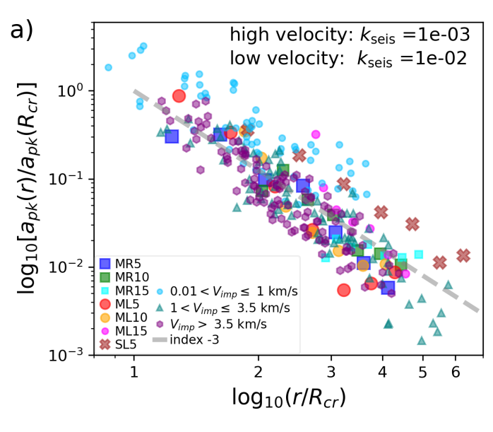
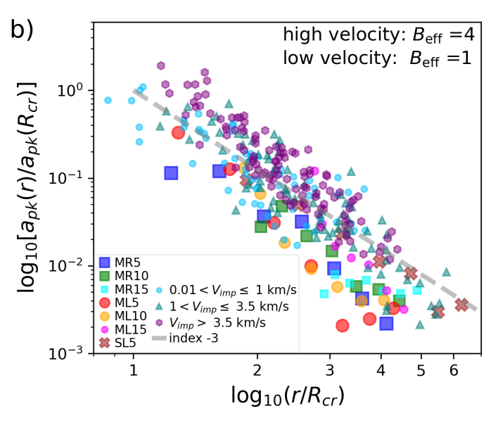
Figure 18: a) Normalized peak accelerations as a function of distance from impact divided by crater radius. The peak accelerations have been divided by $a_{pk}(R_{cr})$ computed using equation 42 and with impact kinetic energy, crater radius, pulse travel velocity and substrate density for each experiment. The seismic efficiency parameter $k_{seis}$ we use for our low velocity experimental measurements and for the high velocity experimental measurements by Yasui et al. (2015) and Matsue et al. (2020) are printed on the upper right and are also listed in Table 7. The dashed grey line shows $a_{pk}(r)/a_{pk}(R_{cr})=(r/R_{cr})^{-3}$. The point types for our data (the low velocity experiments) are the same as shown in Figure 8. The point types for the high velocity experiments are the same as in Figure 11. b) similar to a) except equation 45 is used to compute the normalization for the acceleration. This depends on the momentum transfer parameter $B_{\rm eff}$ which is printed on the upper right.

Table 7: Values for estimating quantities at the crater radius

Parameter	$b_{\rm eff}C_{D}$	$k_{seis}$	$B_{\rm eff}$
Description	Momentum transf. times drag coeff.	Momentum transfer efficiency	Seismic efficiency parameter
Expression	Eqn. (30)	Eqn. (41)	Eqn. (44)
Slow impacts	4 to 7	$10^{-2}$	1
Fast impacts	0.1 to 0.005	$10^{-3}$	4

5 The pulse excited by the DART impact on Dimorphos

In Sept. 2022, the DART spacecraft will impact the secondary of the asteroid (65803) Didymos system, known as Dimorphos. Using the diffusive model developed in Section 4, we estimate the characteristics of a seismic pulse that is driven by the impact. The DART impact velocity will be about $v_{imp}\approx 6.5$ km/s and the impactor mass at the time of impact is expected to be about $m_{p}\approx 550$ kg (Rivkin et al., 2021). This gives a kinetic energy of $K_{imp}\approx 1.2\times 10^{10}$J.

The mass and radius of the target, Dimorphos, are estimated to be $m_{a}\approx 5\times 10^{9}$ kg and $R_{a}\sim 80$ m (Naidu et al., 2020). Dimorphos’ density is based on estimates of the density of the primary, Didymos, $\rho_{s}\approx 2.17$ g cm^-3 (Naidu et al., 2020). The gravitational acceleration on the surface of Dimorphos $g_{\rm eff}\sim Gm_{a}/R_{a}^{2}\sim 5\times 10^{-5}{\rm m\ s}^{-2}$.

The material properties of Dimorphos could resemble those of the recently well characterized rubble NEA asteroid (101955) Bennu. The bulk mass density of Bennu is $\rho=1.190\pm$ 13 g cm^-3 (Lauretta et al., 2019). Tricarico et al. (2021) estimate a rubble bulk density (that of the rubble pieces inside the asteroid) of 1.35 g/cm³. This is somewhat higher than the bulk density of the asteroid itself 1.19 g/cm³ including voids, so Tricarico et al. (2021) estimate moderate macro-porosity of about 12% (corresponding to voids between rocks). As the rubble bulk density is lower than that of representative meteoritic samples, $\sim 3$ g/cm³ (see Macke et al. 2011), Tricarico et al. (2021) infer that the rocks themselves are likely to exhibit micro-porosity $\sim$ 50%. This high porosity is similar to the porosity of some meteoritic samples (Macke et al., 2011). Seismic wave velocity for rocks is reduced, compared to that of solid constituents, due to porosity and the nature and density of internal voids and cracks (O’Connell and Budianski, 1974; Kovacic, 1999). Because Dimorphos’s rocks are likely to be porous, we estimate the elastic modulus of the grain material to be low, $E_{g}\sim 10$ GPa, and similar to that of some sandstones. At a density of 2 g/cm^-3, this gives a sound speed within each rock or grain of $c_{g}\sim\sqrt{E_{g}/\rho_{s}}\sim 2000$ m/s.

Because Dimorphos is a low-g environment, pulse propagation should be a regime with velocity that depends on peak pressure in the pulse, so we adopt the pressure dependent scaling by van den Wildenberg et al. (2013) which is based on experiments into polydisperse glass beads. The relation is

$$\frac{v_{P}}{c_{g}}\sim\left(\frac{P_{pk}}{E_{g}}\right)^{\frac{1}{6}}.$$ (46)

To order of magnitude this relation is similar to the $v_{P}/c_{g}$ vs $P_{0}/E_{g}$ relation by Jia et al. (1999) for disordered glass spheres that depends upon confinement pressure rather than peak pressure. Equation 46 along with Equation 5, gives a relation between peak pressure and peak velocity in a traveling longitudinal pressure pulse

$$P_{pk}\sim\left[\rho_{s}v_{pk}c_{g}\right]^{\frac{6}{5}}E_{g}^{-\frac{1}{5}}.$$ (47)

With gravity inversion methods, Tricarico et al. (2021) find that the rubble size frequency distribution of the interior of asteroid (101955) Bennu is consistent with that observed on the surface, with a cumulative index of approximately $-2.9$ (DellaGiustina et al., 2019). With this index, the mean particle size is set by the smallest particles whereas the mean particle volume is set by the largest particles. Since, the largest particles carry the strong force chains (Voivret et al., 2009), the larger particles could set the properties of seismic attenuation within the medium. The particle size distribution seen on the surface has a number of particles with diameters of 50 m, so we use that as a size-scale to estimate a diffusion coefficient related to pulse broadening. For a fiducial value, we use a diffusion coefficient in the form of Equation 22 with $D/v_{P}=C_{W}^{2}d_{g}=10^{3}$ m. We use a large value so as to be consistent with the values we estimated for $C_{W}\sim 10$ from our experiments described in sections 3.9 and 4.

Localization of seismic waves generated by hypervelocity (velocity of greater than a km/s) impacts into sandstone gives impact site as origin (Moser et al., 2013). Even though our experiments show anisotropy in pulse strength, we adopt a model where pulse strength only depends on travel distance $r$ from the site of impact (and following Thomas and Robinson 2005). We assume that the transition to a propagating seismic pulse takes place at a distance near the crater radius. As done in Section 4, we scale properties of the travel seismic pulse from the crater radius, at a distance $r=R_{cr}$. The radius of the impact crater on Dimorphos that will be caused by the DART impact has been estimated with scaling laws (Housen and Holsapple, 2011) and ranges from $R_{cr}\sim$ 4 to 45 m, with value that depend upon the substrate material properties (Cheng et al., 2016, 2020). For a fiducial value we adopt $R_{cr}=10$ m.

Because a seismic source time gave pulse duration similar to that observed in both our experiments and those by Yasui et al. (2015) and Matsue et al. (2020), we use it to estimate the pulse duration at a distance of the crater radius from the site of the DART impact. We assume that the pulse width at the crater radius is

$$\Delta t_{v}(R_{cr})\sim\frac{R_{cr}}{v_{P}(R_{cr})}.$$ (48)

The seismic efficiency in the high velocity DART impact should be lower than the seismic efficiency measured in our low velocity experiments because energy would be lost during shock propagation and while the pressure wave propagates in a plastic regime (Shishkin, 2007; Güldermeister and Wünnemann, 2017). We adopt a fiducial value for the seismic efficiency $k_{seis}\sim 10^{-3}$, following the estimates and measurements by Shishkin (2007); Güldermeister and Wünnemann (2017) and approximately consistent with the high velocity laboratory impacts by Yasui et al. (2015) and Matsue et al. (2020). Equation 36 for the seismic energy at a distance $r=R_{cr}$ and pulse width from equation 48, gives equations 39 and 40, and these give peak pulse velocity at the crater radius in equation 42. Using values for the DART impact and equation 42 we estimate the peak pulse velocity at the crater radius

$$v_{pk}(R_{cr})\sim \sqrt{\frac{k_{seis}K_{imp}}{2\pi R_{cr}^{3}\rho_{s}}}$$

$$= 1.0\ {\rm m/s}\left(\frac{k_{seis}}{10^{-3}}\right)^{\frac{1}{2}}\!\left(\frac{K_{imp}}{1.2\times 10^{10}{\rm J}}\right)^{\frac{1}{2}}\times$$

$$\ \ \left(\frac{\rho_{s}}{2000\ {\rm kg\ m}^{3}}\right)^{-\frac{1}{2}}\!\left(\frac{R_{cr}}{10\ {\rm m}}\right)^{-\frac{3}{2}}.$$ (49)

Instead of scaling from seismic energy, we could use the momentum of impact $m_{p}v_{imp}$ and a momentum transfer efficiency parameter $B_{\rm eff}$ to characterize the fraction of momentum that is transferred into a seismic pulse. Hypervelocity impact experiments into pumice estimate a recoil from crater ejecta that exceeds the direct momentum transferred by absorption of the projectile by a factor of order unity (e.g., Flynn et al. 2015), though $B_{\rm eff}\sim 4$ is more consistent with the high velocity laboratory experiments by Yasui et al. (2015) and Matsue et al. (2020), as we discussed in section 4.3. Equation 24 for the momentum in the pulse and using equation 48 for the pulse width, gives a peak velocity at the crater radius in equation 45. Using values for the DART impact

$$v_{pk}(R_{cr}) \sim\frac{B_{\rm eff}m_{p}v_{imp}}{\rho_{s}2\pi R_{cr}^{3}}$$

$$\sim 0.28{\rm m/s}\left(\frac{B_{\rm eff}}{1}\right)\!\left(\frac{m_{p}v_{imp}}{3.6\times 10^{6}\ {\rm kg\ m\ s}^{-1}}\right)\!$$

$$\ \ \left(\frac{\rho_{s}}{2000\ {\rm kg\ m}^{3}}\right)^{-1}\!\!\ \ \left(\frac{R_{cr}}{10\ {\rm m}}\right)^{-3}.$$ (50)

As this is similar in size to Equation 49, either the momentum transfer efficiency parameter $B_{\rm eff}$ or seismic efficiency $k_{seis}$ can be used to estimate the peak velocity $v_{pk}(R_{cr})$. Equations 46, 47, 48 and 49 are sufficient to estimate other physical quantities at $r=R_{cr}$. Pulse amplitude and other quantities at the crater radius approximately scale with our initial choice of crater radius in the following manner; $v_{pk}(R_{cr})\propto R_{cr}^{-\frac{3}{2}}$ (from equation 49), $P_{pk}(R_{cr})\propto R_{cr}^{-\frac{9}{5}}$ (following equation 47), $v_{P}(R_{cr})\propto R_{cr}^{-\frac{3}{10}}$ (following equation 46), $\Delta t_{v}(R_{cr})\propto R_{cr}^{\frac{13}{10}}$ (following equation 48), $a_{pk}(R_{cr})\sim v_{pk}/\Delta t_{v}\propto R_{cr}^{-\frac{14}{5}}$, and $\delta_{pk}(R_{cr})\sim v_{pk}\Delta t_{v}\propto R_{cr}^{-\frac{1}{5}}$. The seismic energy is fixed by the seismic efficiency (following equation 39).

If attenuation is directly related to pulse duration, then with an assumption for the form of the diffusion coefficient, we can estimate how the generated pulse broadens as it travels. Using the diffusive model discussed in Section 4, the square of the pulse duration for a pulse that propagates from $r=R_{cr}$

$$[\Delta t_{v}(r)]^{2} =[\Delta t_{v}(R_{cr})]^{2}+\int_{R_{cr}}^{r}dr\frac{D}{v_{P}(r)^{3}}.$$ (51)

We use diffusion coefficient $D$ in the form of Equation 22 for a propagation velocity that depends on pulse amplitude (or the peak pressure in the pulse).

As in Section 4, we assume that the radial component of momentum per unit solid angle is approximately conserved while the pulse propagates. Equation 24 and Equation 5 give peak pulse pressure

$$P_{pk}(r) \sim P_{pk}(R_{cr})\left(\frac{R_{cr}}{r}\right)^{2}\left(\frac{\Delta t_{v}(R_{cr})}{\Delta t_{v}(r)}\right).$$ (52)

By integrating Equation 51 while updating the peak pressure $P_{pk}$ with Equation 52, and using Equations 46 and 47 for $v_{P}$ and $P_{pk}$, we can compute physical quantities such as $v_{P}$, $v_{pk}$ as a function of distance from the site of impact. A resulting integration is shown in Figure 19 with fiducial parameters summarized in Table 8. In this figure we plot pulse peak pressure $P_{pk}$, peak acceleration $a_{pk}$, peak velocity $v_{pk}$, peak displacement $\delta_{pk}$, pulse velocity $v_{P}$ and pulse duration $\Delta t_{v}$. These quantities are plotted as a function of travel distance from the site of impact $r$. We only plot quantities for $r>R_{cr}$ as pulse properties are scaled from our estimates at the crater radius, $r=R_{cr}$. The plot is limited to $r<2R_{a}$ where $R_{a}$ is the estimated radius of Dimorphos.

The fiducial model in Figure 19 shows that the diffusive spreading rapidly dominates the pulse duration. Past about $r\sim 2R_{cr}$, the pulse width approximately scales with $r^{\frac{1}{2}}$, similar to that obeyed by our model in Section 4 where pulse velocity $v_{P}$ is constant. Here the pulse travel speed decreases as the pulse travels, but because it is only weakly dependent on pulse pressure (to the 1/6–th power), $v_{P}$ only varies slowly with $r$. This implies that the power law indices for pulse properties that we previously estimated in Section 4 as a function of travel distance $r$ will also be obeyed in the model discussed here; $v_{pk},P_{pk},E_{seis}\propto r^{-\frac{5}{2}}$, $a_{pk}\propto r^{-3}$, $\delta_{pk}\propto r^{-2}$, and $\Delta t_{v}\propto r^{\frac{1}{2}}$. This also implies that the magnitudes of the estimated physical quantities are not strongly dependent upon the assumed index of 1/6.

From Figure 19, we estimate a surface displacement in the seismic pulse of only a few cm at $r\approx R_{cr}$. LICIACube will have a flyby distance of 55 km, and its imagery should have a resolution at closest approach of 1.4 m pixel^-1 (Dotto et al., 2021). Boulder displacements in the seismic pulse itself are a few cm large at $r=R_{cr}$ and so would be about two orders of magnitude out of reach of LICIACube’s imaging. Accelerations caused by the seismic pulse should be significant compared to the surface gravity. For our fiducial model, $a_{pk}>g_{\rm eff}$, peak acceleration exceeds the surface gravity of the asteroid (about $0.5\times 10^{-4}$ m/s²), for a travel length equal to asteroid diameter. Despite rapid attenuation, particles on the surface would be perturbed all over the asteroid. Only near the crater would peak pulse velocities be similar to the escape velocity, which on Dimorphos is about 10 cm/s, as expected for formation of the crater.

In Figure 20 we show peak accelerations for models similar to the fiducial one. We vary a single parameter in each model. We also show a constant pulse velocity model with $v_{P}=100$ m/s that is independent of pulse amplitude. Reducing the grain elastic modulus has the same effect as reducing $v_{P}$. The pulse is stronger with a smaller diffusion coefficient and if the crater radius is large. All of the models shown in Figure 20 show peak accelerations above the surface effective gravity $g_{\rm eff}$ for travel distances that are similar to the radius of the asteroid. Despite the high level of attenuation implied by our diffusive model, the seismic pulse traverses the asteroid and can cause significant surface motions that can disturb the surface.

When they reach a granular surface, a strong seismic pulse can cause the surface to deform, induce landslides and loft particles off the surface (e.g., Tancredi et al. 2012; Wright et al. 2020). These processes would also reduce the amplitude of reflected waves and increase the attenuation rate. After the pulse has traversed the asteroid, seismic energy would continue to attenuate and peak accelerations would drop below $g_{\rm eff}$. The impact generated pulse would only be strong enough to disturb the surface during a single crossing time. The scenario is consistent with the seismic jolt model used to account for crater erasure on Eros with a single seismic pulse (Thomas and Robinson, 2005).

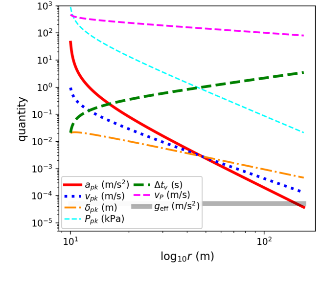
Figure 19: Quantities estimated for a pulse excited by the DART impact into Dimorphos as a function of distance from the site of impact. Parameters for this model are listed in Table 8. The model was created by integrating Equation 51 and using Equations 52, 46, 47 and values at the crater radius based on Equations 48 and 49. The thick grey line shows the surface gravity of Dimorphos, $g_{\rm eff}$ in m/s².

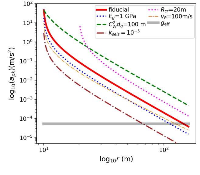
Figure 20: Pulse peak acceleration as a function of distance from impact for DART impulse models. The fiducial model, here shown with a solid red line, is the same as that shown in Figure 19 and with parameters listed in Table 8. The other lines show models that are like the fiducial model except a single parameter is changed. The new parameter value for each model is shown in the key. We also show a diffusive and constant pulse velocity ($v_{P}$) model. The thick grey line shows the gravitational acceleration at the surface of Dimorphos.

Table 8: DART impulse fiducial model

Quantity		Value
Kinetic energy of impact	$K_{imp}$	$1.2\times 10^{10}$ J
Seismic efficiency	$k_{seis}$	$10^{-3}$
Bulk density	$\rho_{s}$	2000 kg m-3
Substrate elastic modulus	$E_{g}$	10 GPa
Crater radius	$R_{cr}$	10 m
Diffusion coef. parameter	$\frac{D}{v_{P}}=C_{W}^{2}d_{g}$​​​​	1000 m

6 Summary and Discussion

In this paper we have used an array of 7 accelerometers to characterize propagation and decay of a pulse excited in a granular medium by a low velocity normal impact. Our impact velocity is about 5 m/s and our impacts take place into millet or fine sand that fill an approximately cylindrical 41.6 litre tub. Our experiments are complimentary to those by Yasui et al. (2015) and Matsue et al. (2020) as they are at lower velocity, in different granular substrates, and measure pulse properties at more accelerometer positions.

The accelerometers primarily detect a longitudinal pressure pulse that propagates radially away from the site of impact. We estimate that a seismic pulse is launched within a few ms from the moment of impact. The pulse travel speed is similar in millet and fine sand, and about 55 m/s and matches that seen by Matsue et al. (2020) in 100 m/s impact experiments into quartz sand. The pulse travel speed in units of the sound speed within the grains for both substrates is approximately consistent with predictions and experimental measurements of pressure dependent wave propagation in a disordered granular medium (Jia et al., 1999; Somfai et al., 2005; van den Wildenberg et al., 2013).

We examined the orientation of the peak accelerations. Acceleration vectors are oriented radially with origin at the site of impact. This implies that we primarily see longitudinal wave propagation. If asteroid material behaves similarly, we would not expect to see phenomena on rubble asteroids that is associated with shear waves, such as Rayleigh waves or antipodal focusing, though jamming associated with shear stress (Bi et al., 2011) could be relevant for pulse generation in granular media.

Pulses in our experiments broaden, become smoother and rapidly attenuate as they travel away from the impact site. Pulse propagation is not spherically symmetric about the site of impact. Pulse peak velocities are about twice as large along a direction directly down compared to those along a direction of about 45^∘ from vertical. This behavior may be similar to phenomena seen in simulations of oblique impacts that showed plastic deformation within the granular medium extending further laterally than vertically, and led to a more rapid decay of energy in the lateral pulse compared to the vertical pulse (Miklavcic et al., 2022).

We measure a pulse duration of approximately 1 ms which most closely matches a seismic source time equal to the crater size divided by the pulse travel speed. This suggests that this time is relevant for pressure release within the material during crater formation. To within a factor of a few, the hypothesis that the seismic source time is similar to the pulse duration is supported by the experimental measurements of pulse duration in higher velocity experiments by Yasui et al. (2015) and Matsue et al. (2020). The pulses in sand were about half as long as those in millet, suggesting that pulse duration could also be sensitive to grain size. Our pulse durations could also be consistent with an initially short duration pulse (less than 1 ms) and subsequent broadening, but only if the diffusion coefficient (for propagating velocity or pressure perturbations) is about an order of magnitude larger than expected from the experiments of weak pulses into granular media by Langlois and Jia (2015).

Our detected acceleration and velocity signals exhibit attenuation and broadening. Pulse shapes become smoother as they propagate. Because these are characteristics of diffusive behavior we adopted a diffusive rather than dispersive model for pulse propagation. Using a simple diffusive model for pulse broadening, we estimate that the peak pulse velocity, pressure and seismic energy are proportional to $r^{-\frac{5}{2}}$ and the peak acceleration $\propto r^{-3}$ where $r$ is distance from site of impact. The predicted power law index of -3 is consistent with decay of peak acceleration measured in higher velocity experiments by Matsue et al. (2020). Our measurements are roughly consistent with these exponents for signals from accelerometers near the impact site where the pulses are stronger and less affected by reflections from the container base or walls. These decay exponents are steeper than predicted or measured in impacts into solids for pulse travel in the elastic regime (Güldermeister and Wünnemann, 2017). The rapid attenuation in our experiments supports a seismic jolt model for impact excited pulse propagation in rubble asteroids (Nolan et al., 1992; Greenberg et al., 1994, 1996; Nolan et al., 2001; Thomas and Robinson, 2005) and does not support the slowly attenuating seismic reverberation model (Cintala et al., 1978; Cheng et al., 2002; Richardson et al., 2004, 2005; Yamada et al., 2016).

Past about 5 ms after impact, our pulses can reach tub walls and base. A positive pressure pulse can reflect off a hard wall in a granular medium. We do detect accelerations after 5 ms but they decay rapidly. We have not tried to model the behavior of the accelerations at later times because the signals decay rapidly and so are weak at later times, because reflections are complicated by flexure in the tub and because vibrational energy is absorbed through the tub base. Nevertheless the rapid decay of seismic energy in the medium at later times is not inconsistent with the rapid decay of energy at earlier times. After 2 tub crossing times, signals are sufficiently weak that we cannot determine if there are reflections off the granular surface. Because material can be ejected from a granular surface by a positive pressure pulse (Wright et al., 2020), we expect that seismic energy would be absorbed rather than reflected by the free granular surface. This could also be true in a low g environment such as a rubble asteroid (Tancredi et al., 2012).

Using the kinetic energy in the pulse measured from the accelerometer nearest the impact site, we estimate a seismic efficiency $k_{seis}$ of about a percent at a distance from impact site that is just outside the crater radius. This seismic efficiency value is high compared to the higher velocity impact experiments into granular media by Yasui et al. (2015). However, as attenuation is rapid, the estimated seismic efficiency is sensitive to the distance at which seismic energy is measured. Pulse strength might be better characterized by the ratio of the momentum that goes into the pressure pulse and that of the impactor (our $B_{\rm eff}$ parameter) than the seismic efficiency parameter ($k_{seis}$).

We apply our diffusive propagation model to estimate the size and exponents for decay of pulse physical properties for the pulse excited by the forthcoming DART impact into Dimorphos, the secondary of the asteroid Didymos. We made the following assumptions: The asteroid Dimorphos is comprised of rubble. We adopt a pressure dependent pulse travel speed based on studies of granular systems (van den Wildenberg et al., 2013). The initial pulse width is set by the seismic source time at the crater radius. The pulse width subsequently broadens via a diffusive approximation with diffusion coefficient given by Equation 22. The radial component of momentum integrated at the pulse front per unit solid angle is conserved. We assume that the seismic pulse propagates isotropically as a function of $r$. By scaling from properties at a distance $r=R_{cr}$ equal to the crater radius from the site of impact, we ignore the details of the early phases of the impact that would include vaporization, melting and strong shocks.

The resulting models exhibit rapid attenuation of seismic energy due to pulse broadening. The models resemble a constant pulse velocity diffusive model which we compared to our experiments in Section 4 and which have peak pulse pressure decaying as a function of travel distance from site of impact in power-law form $P_{pk}\propto r^{-\frac{5}{2}}$. Using parameters estimated for the DART impact, and despite assuming a high diffusion coefficient, we estimate that pulse peak accelerations will exceed surface gravity as the pulse travels through the asteroid. Because the surface of a granular system would have little cohesion, we expect that the asteroid surface will absorb seismic energy by lofting and disturbing surface particles. We do not expect a reflected pulse, so pulse strength will be negligible after a single crossing of the asteroid and there will not be much reverberation. Material on the surface could be disturbed over a large fraction of the asteroid surface prior to the landing of crater ejecta. The impact could be nearly catastrophic, in the sense that a significant layer of asteroid material would be lofted from the surface by the seismic pulse, though most of this material should return to re-accumulate on the core. Our experiments suggest that the pulse amplitude could be dependent on propagation angle, so some regions of the asteroid surface could be more strongly disturbed by the seismic pulse than others.

There is a discrepancy in our experiments between the strength of diffusion and those estimated in the experiments by Langlois and Jia (2015). While we took into account the pressure dependence of the pulse travel speed (van den Wildenberg et al., 2013) in our rough estimate for the properties of the impulse excited by the DART impact, we neglected a possible pressure dependence of the diffusion or attenuation rate. A dependence of the broadening rate on pulse peak pressure might account for our high estimated diffusion coefficients compared to other experiments. We estimate that, in our experiments, pulse peak pressures exceed hydrostatic pressure within about 10 cm of the impact site. Our pressure pulses are just barely in a regime that is relevant for a low-g environment. Perhaps the regime with peak pressure larger than hydrostatic pressure $P_{pk}>P_{0}$, which is relevant for low g environments, exhibits faster broadening than outside this regime, with peak pulse pressure below hydrostatic or confining pressure, $P_{pk}<P_{0}$. Future studies could better characterize the dependence of the attenuation or diffusion rate on the pulse amplitude. Our experiments suggest that the rate of pulse broadening and attenuation is sensitive to grain size. Future work could study how grain properties (friction coefficients, elastic modulus) and shape, size and composition distributions affect propagation of impact generated pulses.

Our experiments show that pulse amplitude depends on the direction of propagation and is higher normal to the surface (downward in our experiment). Future studies could improve measurements of the angular dependence of impact generated pulses and study simulations to learn how impact generated pulses depend on propagation angle from the surface normal, the impact angle and the surface slope.

We adopted a diffusive empirical model to describe pulse broadening and attenuation in part because of its simplicity. With a few assumptions and free parameters, pulse properties can be predicted as a function of travel distance from site of impact by scaling from values at the crater radius. If a diffusive model gives an approximate description of pulse propagation in granular media, it would be powerful because of its simplicity.

In our model for the DART impact, we assumed that pulse propagation in rubble in low g primarily is dependent on the peak pressure in the seismic pulse, following van den Wildenberg et al. (2013). Dimensionless numbers indirectly enter into our pulse propagation model because we scaled the model from properties estimated at the crater radius which obeys crater scaling relations (Holsapple, 1993; Housen and Holsapple, 2003; Yasui et al., 2015). If pulse propagation is primarily dependent on peak pulse pressure, then our diffusive approximation can be directly applied to low g environments. However, pulse propagation within granular systems is nonlinear and possibly dispersive as well as advective and diffusive, so future studies could test the validity of the approximations we have adopted here and their application to low g environments.

Acknowledgements:

This material is based upon work supported in part by NASA grant 80NSSC21K0143, and National Science Foundation Grant No. PHY-1757062. This work was supported in part by an award to J. South from the Rochester Academy of Sciences for purchase of granular materials. This work was supported in part by undergraduate research awards from the University of Rochester to J. South and N. Skerrett. We thank Anton Peshkov for helpful discussions and correspondence. We thank Jiaxin Wang for helping us in the lab. We thank Jack Mottley for advice on pulse generation techniques.

6.1 Nomenclature

Table 9: Nomenclature

Drop height	$h_{drop}$
Projectile mass	$m_{p}$
Projectile radius	$R_{p}$
Projectile density	$\rho_{p}$
Projectile velocity	$v_{p}$
Projectile inverse stopping length	$\alpha_{p}$
Impact velocity	$v_{imp}$
Kinetic energy of impact	$K_{imp}$
Froude number	$Fr$
Dimensionless numbers	$\pi_{2},\pi_{R},\pi_{4}$
Ambient or hydrostatic pressure	$P_{0}$
Peak pressure in a pulse	$P_{pk}$
Peak velocity in a pulse	$v_{pk}$
Peak acceleration in a pulse	$a_{pk}$
Peal displacement in a pulse	$\delta_{pk}$
Pulse propagation speed	$v_{P}$
Depth	$H$
Distance from impact site	$r$
Crater radius	$R_{cr}$
Crater diameter	$D_{cr}$
Gravitational acceleration on Earth	$g_{\oplus},g$
Surface gravitational acceleration	$g_{\rm eff}$
Radial velocity component	$v_{r}$
Radial acceleration component	$a_{r}$
Time of propagation	$t_{prop},t_{a,prop},t_{v,prop}$
Pulse duration	$\Delta t,\Delta t_{a},\Delta t_{v}$
Normalized pulse duration	$W,W_{a},W_{v}$
Spatial pulse width	$\Delta r$
Diffusion coefficient	$D$
Diffusion scaling coefficient	$C_{W}$
Bulk density of substrate	$\rho_{s}$
Grain diameter	$d_{g}$
Grain elastic modulus	$E_{g}$
Sound speed in the grain’s material	$c_{g}$
Drag coefficient	$C_{D}$
Seismic energy	$E_{seis}$
Seismic efficiency	$k_{seis}$
Momentum transfer parameters	$b_{\rm eff},B_{\rm eff}$
Asteroid mass	$m_{a}$
Asteroid radius	$R_{a}$
Angle of repose	$\theta_{r}$
Coefficient of friction	$\mu_{s}$

References

- Aki and Richards (2002) Aki, K., Richards, P. G., 2002. Quantitative Seismology, 2nd Edition. University Science Books, Melville, NY.
- Asphaug (2008) Asphaug, E., 2008. Critical crater diameter and asteroid impact seismology. Meteoritics & Planetary Science 43 (6), 1075–1084.
- Bi et al. (2011) Bi, D., Zhang, J., Chakraborty, B., Behringer, R., 2011. Jamming by shear. Nature 480, 355–358.
- Cheng et al. (2002) Cheng, A., Izenberg, N., Chapman, C., Zuber, M. T., 2002. Ponded deposits on Asteroid 433 Eros. Meteoritics & Planetary Science 37, 1095–1105.
- Cheng et al. (2016) Cheng, A. F., Michel, P., Jutzi, M., Rivkin, A., Stickle, A., Barnouin, O., Ernst, C., Atchison, J., Pravec, P., Richardson, D., team, A., team, A., 2016. Asteroid impact & deflection assessment mission: Kinetic Impactor. Planetary and Space Science 121, 27–35.
- Cheng et al. (2018) Cheng, A. F., Rivkin, A. S., Michel, P., Atchison, J., Barnouin, O., Benner, L., Chabot, N. L., Ernst, C., Fahnestock, E. G., Kueppers, M., Pravec, P., Rainey, E., Richardson, D. C., Stickle, A. M., Thomas, C., 2018. AIDA DART asteroid deflection test: Planetary defense and science objectives. Planetary and Space Science 157, 104–115.
- Cheng et al. (2020) Cheng, A. F., Stickle, A. M., Fahnestock, E. G., Dotto, E., Corte, V. D., Chabot, N. L., Rivkin, A. S., dec 2020. DART mission determination of momentum transfer: Model of ejecta plume observations. Icarus 352, 113989.
- Chujo et al. (2018) Chujo, T., Mori, O., Kawaguchi, J., Yano, H., 2018. Categorization of Brazil nut effect and its reverse under less-convective conditions for microgravity geology. Monthly Notices of the Royal Astronomical Society, 474 (4), 4447–4459.
- Cintala et al. (1978) Cintala, M. J., Head, J. W., Veverka, J., 1978. Characteristics of the cratering process on small satellites and asteroids. Proceedings of Lunar Sci. Conf. 9, 3803–3830.
- Coste and Gilles (2008) Coste, C., Gilles, B., 2008. Sound propagation in a constrained lattice of beads: High-frequency behavior and dispersion relation. Phys. Rev. 77, 021302.
- Da Silva and Rajchenbach (2000) Da Silva, M., Rajchenbach, J., 2000. Stress transmission through a model system of cohesionless elastic grains. Nature 406, 708–710.
- Dainty et al. (1974) Dainty, A., Toksöz, M. N., Anderson, K., Pines, P., Nakamura, Y., Latham, G., 1974. Seismic scattering and shallow structure of the Moon in Oceanus Procellarum. Moon 9, 11–29.
- DellaGiustina et al. (2019) DellaGiustina, D. N., , Emery, J. P., Golish, D. R., Rozitis, B., Bennett, C. A., Burke, K. N., Ballouz, R.-L., Becker, K. J., Christensen, P. R., d’Aubigny, C. Y. D., Hamilton, V. E., Reuter, D. C., Rizk, B., Simon, A. A., Asphaug, E., Bandfield, J. L., Barnouin, O. S., Barucci, M. A., Bierhaus, E. B., Binzel, R. P., Bottke, W. F., Bowles, N. E., Campins, H., Clark, B. C., Clark, B. E., Connolly, H. C., Daly, M. G., de Leon, J., Delbo’, M., Deshapriya, J. D. P., Elder, C. M., Fornasier, S., Hergenrother, C. W., Howell, E. S., Jawin, E. R., Kaplan, H. H., Kareta, T. R., Corre, L. L., Li, J.-Y., Licandro, J., Lim, L. F., Michel, P., Molaro, J., Nolan, M. C., Pajola, M., Popescu, M., Garcia, J. L. R., Ryan, A., Schwartz, S. R., Shultz, N., Siegler, M. A., Smith, P. H., Tatsumi, E., Thomas, C. A., Walsh, K. J., Wolner, C. W. V., Zou, X.-D., Lauretta, D. S., mar 2019. Properties of rubble-pile asteroid (101955) Bennu from OSIRIS-REx imaging and thermal analysis. Nature Astronomy 3 (4), 341–351.
- Dotto et al. (2021) Dotto, E., Della Corte, V., Amoroso, M., Bertini, I., Brucato, J., Capannolo, A., Cotugno, B., Cremonese, G., Di Tana, V., Gai, I., Ieva, S., Impresario, G., Ivanovski, S., Lavagna, M., Lucchetti, A., Mazzotta Epifani, E., Meneghin, A., Miglioretti, F., Modenini, D., Pajola, M., Palumbo, P., Perna, D., Pirrotta, S., Poggiali, G., Rossi, A., Simioni, E., Simonetti, S., Tortora, P., Zannoni, M., Zanotti, G., Zinzi, A., Cheng, A., Rivkin, A., Adams, E., Reynolds, E., Fretz, K., 2021. LICIACube - the Light Italian Cubesat for imaging of asteroids in support of the NASA DART mission towards asteroid (65803) Didymos. Planetary and Space Science 199, 105185.
- Duffy and Mindlin (1957) Duffy, J., Mindlin, R., 1957. Stress-strain relations and vibrations of a granular medium. J. Appl. Mech. 24, 585–593.
- Flynn et al. (2015) Flynn, G. J., Durda, D. D., Patmore, E. B., Clayton, A. N., Jack, S. J., Lipman, M. D., Strait, M. M., 2015. Hypervelocity cratering and disruption of porous pumice targets: Implications for crater production, catastrophic disruption, and momentum transfer on porous asteroids. Planetary and Space Science 107, 64–76.
- Forterre and Pouliquen (2008) Forterre, Y., Pouliquen, O., 2008. Flows of dense granular media. Annual Review of Fluid Mechanics 40, 1–24.
- GDR-MiDi (2004) GDR-MiDi, 2004. On dense granular flows. European Journal of Physics 14, 345–365.
- Geng et al. (2003) Geng, J., Reydellet, G., Clement, E., Behringer, R. P., 2003. Green’s function measurements of force transmission in 2d granular materials. Physica D 182, 274–303.
- Gilles and Coste (2003) Gilles, B., Coste, C., 2003. Low-frequency behavior of beads constrained on a lattice. Phys. Rev. Lett. 90, 174302.
- Goddard (1990) Goddard, J., 1990. Nonlinear elasticity and pressure-dependent wave speeds in granular media. Proc. Roy. Soc. Lond. Math. Phys. Sci. 430, 105–131.
- Goldman and Umbanhowar (2008) Goldman, D. I., Umbanhowar, P., 2008. Scaling and dynamics of sphere and disk impact into granular media. Physics Review E 77, 021308.
- Gómez et al. (2012) Gómez, L. R., Turner, A. M., van Hecke, M., Vitelli, V., 2012. Shocks near jamming. Phys. Rev. Lett. 108, 058001.
- Greenberg et al. (1996) Greenberg, R., Bottke, W., M., N., Geissler, P., Petit, J., Durda, D., Asphaug, E., Head, J., 1996. Collisional and dynamical history of Ida. Icarus 120, 106–118.
- Greenberg et al. (1994) Greenberg, R., Nolan, M., Bottke, W., Kolvoord, R., Veverka, J., 1994. Collisional history of Gaspra. Icarus 107, 84–97.
- Güldermeister and Wünnemann (2017) Güldermeister, N., Wünnemann, K., 2017. Quantitative analysis of impact-induced seismic signals by numerical modeling. Icarus 296, 15–27.
- Herbold et al. (2009) Herbold, E., Kim, J., Nesterenko, V., Wang, S., Daraio, C., 2009. Pulse propagation in a linear and nonlinear diatomic periodic chain: Effects of acoustic frequency band-gap. Acta Mech. 205, 85–103.
- Holsapple (1993) Holsapple, K. A., 1993. The scaling of impact processes in planetary sciences. Annual Review of Earth and Planetary Sciences 21, 333–373.
- Holsapple and Housen (2012) Holsapple, K. A., Housen, K. R., 2012. Momentum transfer in asteroid impacts. i. theory and scaling. Icarus 221, 875–887.
- Hostler and Brennen (2005) Hostler, S. R., Brennen, C. E., 2005. Pressure wave propagation in a granular bed. Physical Review E 72, 031303.
- Housen and Holsapple (2003) Housen, K., Holsapple, K., 2003. Impact cratering on porous asteroids. Icarus 163, 102–119.
- Housen and Holsapple (2011) Housen, K. R., Holsapple, K. A., 2011. Ejecta from impact craters. Icarus 211, 856–875.
- Jia (2004) Jia, X., 2004. Codalike multiple scattering of elastic waves in dense granular media. Physical Review Letters 93, 154303.
- Jia et al. (1999) Jia, X., Caroli, C., Velicky, B., 1999. Ultrasound propagation in externally stressed granular media. Phys. Rev. Lett. 82, 1863.
- Johnson et al. (2000) Johnson, D. L., Makse, H. A., Gland, N., Schwartz, L., 2000. Nonlinear elasticity of granular media. Physica B 279, 134–138.
- Jutzi and Michel (2014) Jutzi, M., Michel, P., 2014. Hypervelocity impacts on asteroids and momentum transfer. i. numerical simulations using porous targets. Icarus 229, 247–253.
- Katsuragi and Durian (2007) Katsuragi, H., Durian, D. J., 2007. Unified force law for granular impact cratering. Nature Physics 3, 420–423.
- Katsuragi and Durian (2013) Katsuragi, H., Durian, D. J., 2013. Drag force scaling for penetration into granular media. Physical Review E 87 (5), 052208.
- Kovacic (1999) Kovacic, J., 1999. Correlation between young’s modulus and porosity in porous materials. Journal of Material Science Letters 18, 1007–1010.
- Langlois and Jia (2015) Langlois, V., Jia, X., 2015. Sound pulse broadening in stressed granular media. Phys. Rev. E 91, 022205.
- Lauretta et al. (2019) Lauretta, D. S., , DellaGiustina, D. N., Bennett, C. A., Golish, D. R., Becker, K. J., Balram-Knutson, S. S., Barnouin, O. S., Becker, T. L., Bottke, W. F., Boynton, W. V., Campins, H., Clark, B. E., Connolly, H. C., d’Aubigny, C. Y. D., Dworkin, J. P., Emery, J. P., Enos, H. L., Hamilton, V. E., Hergenrother, C. W., Howell, E. S., Izawa, M. R. M., Kaplan, H. H., Nolan, M. C., Rizk, B., Roper, H. L., Scheeres, D. J., Smith, P. H., Walsh, K. J., Wolner, C. W. V., mar 2019. The unexpected surface of asteroid (101955) Bennu. Nature 568 (7750), 55–60.
- Liu and Nagel (1992) Liu, C. H., Nagel, S. R., 1992. Sound in sand. Phys. Rev. Lett. 68, 2301–2304.
- Luding (2005) Luding, S., 2005. Granular media: Information propagation. Nature 435, 159–160.
- Macke et al. (2011) Macke, R. J., Consolmagno, G. J., Britt, D. T., 2011. Density, porosity, and magnetic susceptibility of carbonaceous chondrites. Meteoritics & Planetary Science 46 (12), 1842–1862.
- Matsue et al. (2020) Matsue, K., Yasui, M., Arakawa, M., Hasegawa, S., 2020. Measurements of seismic waves induced by high-velocity impacts: Implications for seismic shaking surrounding impact craters on asteroids. Icarus 338, 113520.
- Matsumura et al. (2014) Matsumura, S., Richardson, D. C., Michel, P., Schwartz, S. R., Ballouz, R.-L., 2014. The Brazil nut effect and its application to asteroids. Monthly Notices of the Royal Astronomical Society 443, 3368–3380.
- Maurel et al. (2017) Maurel, C., Ballouz, R.-L., Richardson, D. C., Michel, P., Schwartz, S. R., 2017. Numerical simulations of oscillation-driven regolith motion: Brazil-nut effect. Monthly Notices of the Royal Astronomical Society 464, 2866–2881.
- McGarr et al. (1969) McGarr, A., Latham, G., Gault, D., 1969. Meteoroid impacts as sources of seismicity on the Moon. Journal of Geophysical Research 74, 5981–5994.
- Melosh (1989) Melosh, H. J., 1989. Impact cratering: a geologic process. Oxford Monographs on Geology and Geophysics. Oxford University Press, Oxford England.
- Michel et al. (2022) Michel, P., Kueppers, M., Fitzsimmons, A., Green, S., Lazzarin, M., Ulamec, S., Carnelli, I., Martino, P., 2022. The ESA Hera mission: Detailed characterisation of the DART impact outcome and of the asteroid binary (65803) Didymos, in preparation.
- Miklavcic et al. (2022) Miklavcic, P. M., Askari, H., Sanchez, P., Quillen, A. C., Wright, E., 2022. Subsurface dynamics in oblique granular impacts. submitted to Icarus.
- Miyamoto et al. (2007) Miyamoto, H., Yano, H., Scheeres, D. J., Abe, S., Barnouin-Jha, O., Cheng, A. F., Demura, H., Gaskell, R. W., Hirata, N., Ishiguro, M., Michikami, T., Nakamura, A. M., Nakamura, R., Saito, J., Sasaki, S., May 2007. Regolith migration and sorting on asteroid Itokawa. Science 316 (5827), 1011–1014.
- Moser et al. (2013) Moser, D., Güldemeister, N., Wünnemann, K., Grosse, C., 2013. Acoustic emission analysis of experimental impact processes in comparison to ultrasound measurements and numerical modeling. Journal of Acoustic Emission 31, 50–66.
- Murdoch et al. (2017) Murdoch, N., Avila Martinez, I., Sunday, C., Zenou, E., Cherrier, O., Cadu, A., Gourinat, Y., Jun 2017. An experimental study of low-velocity impacts into granular material in reduced gravity. Monthly Notices of the Royal Astrononical Society 468 (2), 1259–1272.
- Naidu et al. (2020) Naidu, S., Benner, L., Brozovic, M., Nolan, M., Ostro, S., Margot, J., Giorgini, J., Hirabayashi, T., Scheeres, D., Pravec, P., Scheirich, P., Magri, C., Jao, J., 2020. Radar observations and a physical model of binary near-earth asteroid 65803 Didymos, target of the DART mission. Icarus 348, 113777.
- Nakamura (1976) Nakamura, Y., 1976. Seismic energy transmission in the lunar surface zone determined from signals generated by movement of lunar rovers. Bulletin of the Seismological Society of America 66 (2), 593–606.
- Nolan et al. (1992) Nolan, M. C., Asphaug, E., Greenberg, R., 1992. Numerical Simulation of Impacts on Small Asteroids. In: AAS/Division for Planetary Sciences Meeting Abstracts #24. Vol. 24 of Bulletin of the American Astronomical Society. p. 959.
- Nolan et al. (2001) Nolan, M. C., Asphaug, E., Greenberg, R., Melosh, H. J., 2001. Impacts on asteroids: fragmentation, regolith transport, and disruption. Icarus 152, 1–15.
- O’Connell and Budianski (1974) O’Connell, R. J., Budianski, B., 1974. Seismic velocities in dry and saturated cracked solids. Journal Geophysical Research 79 (35), 5412–5426.
- O’Donovan et al. (2016) O’Donovan, J., Ibraim, E., O’Sullivan, C., Hamlin, S., Wood, D. M., Marketos, G., 2016. Micromechanics of seismic wave propagation in granular materials. Granular Matter 18, 56.
- Otto et al. (2003) Otto, M., Bouchaud, J. P., Claudin, P., Socolar, J. E., 2003. Anisotropy in granular media: Classical elasticity and directed-force chain network. Physical Review E 67 (3), 031302.
- Owens and Daniels (2011) Owens, E. T., Daniels, K. E., 2011. Sound propagation and force chains in granular materials. Europhys. Lett. 94, 54005.
- Perera et al. (2016) Perera, V., Jackson, A. P., Asphaug, E., Ballouz, R.-L., 2016. The spherical Brazil Nut Effect and its significance to asteroids. Icarus 278, 194–203.
- Petit and Medina (2018) Petit, J. C., Medina, E., 2018. Reduction of the bulk modulus with polydispersity in noncohesive granular solids. Physical Review E 98 (2), 022903.
- Richardson et al. (2004) Richardson, J. E., Melosh, H. J., Greenberg, R., 2004. Impact-induced seismic activity on asteroid 433 Eros: A surface modification process. Science 306, 1526–1529.
- Richardson et al. (2005) Richardson, J. J., Melosh, H. J., Greenberg, R. J., O’Brien, D. P., 2005. The global effects of impact-induced seismic activity on fractured asteroid surface morphology. Icarus 179, 325–349.
- Rivkin et al. (2021) Rivkin, A. S., Chabot, N. L., Stickle, A. M., Thomas, C. A., Richardson, D. C., Barnouin, O., Fahnestock, E. G., Ernst, C. M., Cheng, A. F., Chesley, S., Naidu, S., Statler, T. S., Barbee, B., Agrusa, H., Moskovitz, N., Daly, R. T., Pravec, P., Scheirich, P., Dotto, E., Corte, V. D., Michel, P., Küppers, M., Atchison, J., Hirabayashi, M., aug 2021. The double asteroid redirection test (DART): Planetary defense investigations and requirements. The Planetary Science Journal 2 (5), 173.
- Sanchez and Scheeres (2021) Sanchez, P., Scheeres, D. J., 2021. Seismic waves in the asteroid environment. EPJ Web of Conferences, Powders and Grains 249, 13001.
- Santibanez et al. (2016) Santibanez, F., Zuñiga, R., Melo, F., 2016. Mechanical impulse propagation in a three-dimensional packing of spheres confined at constant pressure. Physical Review E 93 (1), 012908.
- Shinbrot et al. (2017) Shinbrot, T., Sabuwala, T., Siu, T., Lazo, M. V., Chakraborty, P., 2017. Size sorting on the rubble-pile asteroid Itokawa. Physics Reviews Letters 118, 111101.
- Shishkin (2007) Shishkin, N. I., 2007. Seismic efficiency of a contact explosion and a high velocity impact. Journal of Applied Mechanics and Technical Physics 48, 145–152.
- Somfai et al. (2005) Somfai, E., Roux, J.-N., Snoeijer, J. H., van Hecke, M., van Saarloos, W., 2005. Elastic wave propagation in confined granular systems. Phys. Rev. E 72 (021301).
- Sturm et al. (2016) Sturm, S., Kenkmann, T., Hergarten, S., 2016. Ejecta thickness and structural rim uplift measurements of Martian impact craters: implications for the rim formation of complex impact craters. J. Geophys. Res. 121, 1026–1053.
- Tancredi et al. (2012) Tancredi, G., Maciel, A., Heredia, L., Richeri, P., Nesmachnow, S., 2012. Granular physics in low-gravity environments using discrete element method. Monthly Notices of the Royal Astronomical Society 420, 3368–3380.
- Tancredi et al. (2015) Tancredi, G., Roland, S., Bruzzone, S., 2015. Distribution of boulders and the gravity potential on asteroid Itokawa. Icarus 247, 279–290.
- Tell et al. (2020) Tell, K., Dreißigacker, C., Tchapnda, A. C., Yu, P., Sperl, M., 2020. Acoustic waves in granular packings at low confinement pressure. Review of Scientific Instruments 91 (3), 033906.
- Thomas and Robinson (2005) Thomas, P. C., Robinson, M. S., 2005. Seismic resurfacing by a single impact on the asteroid 433 Eros. Nature 436, 366–369.
- Toksöz et al. (1974) Toksöz, M. N., Dainty, A. M., Solomon, S., Anderson, K., 1974. Structure of the Moon. Reviews of Geophysics 12 (4), 539–567.
- Tricarico et al. (2021) Tricarico, P., Scheeres, D., French, A., McMahon, J., Brack, D., Leonard, J., Antreasian, P., Chesley, S., Farnocchia, D., Takahashi, Y., Mazarico, E., Rowlands, D., Highsmith, D., Getzandanner, K., Moreau, M., Johnson, C., Philpott, L., Bierhaus, E., Walsh, K., Barnouin, O., Palmer, E., Weirich, J., Gaskell, R., Daly, M., Seabrook, J., Nolan, M., Lauretta, D., 2021. Internal rubble properties of asteroid (101955) Bennu. Icarus 370, 114665.
- Tsimring and Volfson (2005) Tsimring, L., Volfson, D., 2005. Modelling of impact cratering in granular media. Powder Technology 2, 1215–1223.
- van den Wildenberg et al. (2013) van den Wildenberg, S., van Loo, R., van Hecke, M., 2013. Shock waves in weakly compressed granular media. Phys. Rev. Lett. 111 (21), 218003.
- Veverka et al. (2001) Veverka, J., Thomas, P., Robinson, M., Murchie, S., Chapman, C., Bell, M., Harch, A., , Merline, W., Bell, J., Bussey, B., Carcich, B., Cheng, A., Clark, B., Domingue, D., Dunham, D., Farquhar, R., Gaffey, M., Hawkins, E., Izenberg, N., Joseph, J., Kirk, R., Li, H., Lucey, P., Malin, M., McFadden, L., Miller, J., Owen, W., Peterson, C., Prockter, L., Wellnitz, J. W. D., Williams, B., Yeomans, D., 2001. Imaging of small-scale features on 433 Eros from NEAR: Evidence for a complex regolith. Science 292, 484–488.
- Voivret et al. (2009) Voivret, C., Radjaï, F., Delenne, J. Y., El Youssoufi, M. S., 2009. Multiscale force networks in highly polydisperse granular media. Physical Review Letters 102 (17), 178001.
- Walsh (2018) Walsh, K. J., 2018. Rubble pile asteroids. Annual Review of Astronomy and Astrophysics 56, 593–624.
- Walton (1987) Walton, K., 1987. The effective elastic moduli of a random packing of spheres. J. Mech. Phys. Solids 35, 213 – 226.
- Wright et al. (2022) Wright, E., Quillen, A. C., Sanchez, P., Schwartz, S. R., Nakajima, M., Askari, H., Miklavcic, P., 2022. Ricochets on asteroids II: Sensitivity of laboratory experiments of low velocity grazing impacts on substrate grain size. Icarus, accepted for publication.
- Wright et al. (2020) Wright, E., Quillen, A. C., South, J., Nelson, R. C., Sanchez, P., Martini, L., Schwartz, S., Nakajima, M., Asphaug, E., 2020. Boulder stranding in ejecta launched by an impact generated seismic pulse. Icarus 337, 113424.
- Yamada et al. (2016) Yamada, T. M., Ando, K., Morota, T., Katsuragi, H., 2016. Timescale of asteroid resurfacing by regolith convection resulting from the impact-induced global seismic shaking. Icarus 272, 165–177.
- Yang et al. (2015) Yang, Z., Sun, J., Guo, Y., 2015. Effect of moisture content on compression mechanical properties and frictional characteristics of millet grain. Transactions of the Chinese Society of Agricultural Engineering 31 (23), 253–260.
- Yasui et al. (2015) Yasui, M., Matsumoto, E., Arakawa, M., 2015. Experimental study on impact-induced seismic wave propagation through granular materials. Icarus 260, 320–331.
- Zhai et al. (2020) Zhai, C., Herbold, E. B., Hurley, R. C., 2020. The influence of packing structure and interparticle forces on ultrasound transmission in granular media. Proceedings of the National Academy of Sciences 117 (28), 16234–16242.