Local minimality properties of circular motions in $1/r^{\alpha}$ potentials and of the figure-eight solution of the 3-body problem

Abstract

We first take into account variational problems with periodic boundary conditions, and briefly recall some sufficient conditions for a periodic solution of the Euler-Lagrange equation to be either a directional, a weak, or a strong local minimizer. We then apply the theory to circular orbits of the Kepler problem with potentials of type $1/r^{\alpha},\,\alpha>0$. By using numerical computations, we show that circular solutions are strong local minimizers for $\alpha>1$, while they are saddle points for $\alpha\in(0,1)$. Moreover, we show that for $\alpha\in(1,2)$ the global minimizer of the action over periodic curves with degree $2$ with respect to the origin could be achieved on non-collision and non-circular solutions. After, we take into account the figure-eight solution of the 3-body problem, and we show that it is a strong local minimizer over a particular set of symmetric periodic loops. AMS Subject Classification: 34B15, 49K15, 34C25, 70F10

Keywords: local minimality, calculus of variations, periodic solutions, Kepler problem, figure-eight

1 Introduction

In recent years, new periodic solutions of the Newtonian $N$-body problem have been discovered by means of variational methods. In particular, taking into account $N$ equal unitary masses and denoting by $u=(u_{1},\dots,u_{N}):[0,T]\to\mathbb{R}^{3N}$ their motion, periodic orbits are found as minimizers of the Lagrangian action functional

$${\cal A}(u)=\int_{0}^{T}\bigg{(}\frac{1}{2}\sum_{i=1}^{N}|\dot{u}_{i}|^{2}+\sum_{1\leq i<j\leq N}\frac{1}{|u_{i}-u_{j}|}\bigg{)}dt,$$ (1.1)

on a set $X$ of $T$-periodic loops, see for instance [5, 6, 3, 4, 13, 2, 14], and references therein. Numerical techniques have been developed as well for the computation of these orbits, see for instance [25, 30, 29, 31, 24, 26, 22, 23, 11] and references therein. However, as already noticed in [30], despite the effectiveness of these methods in computing such orbits, they do not ensure that what is computed is actually a minimizer of the action, not even locally. For this reason, we are interested in finding conditions that guarantee the local minimality, that can be used to understand what kind of stationary point has been computed.

In Calculus of Variations, when the action functional is defined on a subset of $C^{1}$ curves $u:[0,T]\to\mathbb{R}^{n}$ such that

$$\begin{cases}u(0)=u_{0},\\ u(T)=u_{T},\end{cases}$$ (1.2)

where $u_{0},u_{T}\in\mathbb{R}^{n}$ are fixed points, the problem is usually called fixed end-point problem or problem of Bolza, and the theory of local minimizers is a very well-known topic. Indeed, the mathematical formulation of the fixed end-point problem started between the 17th and the 18th centuries, when Bernoulli, Leibniz and Newton independently studied the brachistochrone problem [28, 18]. Further developments have been done in the late 18th century and all over the entire 19th century by, for instance, Euler, Lagrange, Legendre, Jacobi, and Weierstrass. In the last century, the fixed end-point problem became a standard topic in Calculus of Variations, being the subject of several classical mathematical textbooks (see for instance [27, 15, 33]). The interested reader can refer to [16] for a detailed chronological history of Calculus of Variations. When the boundary conditions (1.2) change, definitions and proofs have to be adapted and, depending on the problem one is facing, different necessary and sufficient conditions arise. Theories for the positivity of quadratic functionals with disjoined boundary conditions can be found in [35, 10], while the case of general boundary conditions is treated in [39, 10, 9, 32, 37]. Moreover, in [1] the authors give second order minimality conditions for periodic optimal control problems. A theory of weak local minimizers for different boundary condition types can be found in [20, 21], and references therein. A theory of strong local minimizers for disjoined boundary conditions has been developed in [36], and further improvements led to a theory for general boundary conditions in [38]. These two works are both based on the existence of a symmetric solution of a Riccati differential equation which satisfies a specific boundary condition.

In this work, we first recall some sufficient conditions for the local minimality in variational problems with periodic boundary conditions. In particular, we adapt to the periodic case the proof given in [8] for the fixed end-point problem, by providing appropriate boundary conditions of the symmetric solution of the Riccati differential equation. After, we use the theory in two problems of Celestial Mechanics. First, we take into account the circular solutions in potentials of type $1/r^{\alpha}$, $\alpha>0$, where $r$ is the distance from the center. By using numerical computations, we show that they are strong local minimizers for $\alpha>1$, and saddle points for $\alpha\in(0,1)$. Moreover, we present an example with $\alpha\in(1,2)$ where the global minimizer of the action over periodic curves with degree $2$ with respect to the origin is achieved on a non-collision and non-circular solutions. Then, we take into account the figure-eight solution of the 3-body problem (see [5, 25, 31]). By using numerical computations, we show that the figure-eight is not optimal over the entire set of periodic loops, but it becomes a strong local minimizer when additional symmetries are taken into account.

2 Definitions of local minimizers

Let $T>0$, and consider a functional

$$\mathcal{A}(u)=\int_{0}^{T}L(t,u,\dot{u})dt,$$ (2.1)

where $L:[0,T]\times\Omega\to\mathbb{R}$ is a $C^{2}$ function, $T$-periodic in the variable $t$, and $\Omega\subseteq\mathbb{R}^{n}\times\mathbb{R}^{n}$ is an open set. We denote the space of the $C^{1}$ $T$-periodic functions with

$$V=\{u\in C^{1}([0,T],\mathbb{R}^{n}):u(0)=u(T)\},$$ (2.2)

and assume that ${\cal A}$ is defined on a set $X\subseteq V$. We say that $u_{0}\in X$ is a

• global minimum point if ${\cal A}(u)\geq{\cal A}(u_{0})$ for all $u\in X$;

• strong local minimum point if there exists $\varepsilon>0$ such that, for all $u\in X$ satisfying

  $$\left\lVert u-u_{0}\right\rVert_{\infty}<\varepsilon,$$

  we have that ${\cal A}(u)\geq{\cal A}(u_{0})$.

• weak local minimum point if there exists $\varepsilon>0$ such that, for all $u\in X$ satisfying

  $$\left\lVert u-u_{0}\right\rVert_{\infty}+\left\lVert\dot{u}-\dot{u}_{0}\right\rVert_{\infty}<\varepsilon,$$

  we have that ${\cal A}(u)\geq{\cal A}(u_{0})$.

• directional local minimum point if the function

  $$\varphi(s)={\cal A}(u_{0}+sv),$$

  has a local minimum point at $s=0$ for all $v\in V$. Note that, fixed $v\in V$, $\varphi:(-\delta,\delta)\to\mathbb{R}$ is a function of the real variable $s$, defined for $\delta>0$ small enough.

From the classic theory of Calculus of Variations it is well-known that, if $u_{0}$ is a $C^{2}$ local minimum point, then it solves the Euler-Lagrange equation associated to (2.1), i.e.

$$\frac{d}{dt}L_{\dot{u}}\big{(}t,u_{0}(t),\dot{u}_{0}(t)\big{)}=L_{u}\big{(}t,u_{0}(t),\dot{u}_{0}(t)\big{)}.$$ (2.3)

Moreover, $u_{0}$ satisfies a periodic condition on the derivative, i.e.

$$L_{\dot{u}}(0,u_{0}(0),\dot{u}_{0}(0))=L_{\dot{u}}(T,u_{0}(T),\dot{u}_{0}(T)),$$ (2.4)

which leads to

$$\dot{u}_{0}(0)=\dot{u}_{0}(T),$$ (2.5)

under the assumption that $L$ is globally convex in $\dot{u}$. Note that a solution $u_{0}$ of (2.3) is a (DLM) if and only if the second variation

$$\delta^{2}{\cal A}(v)=\int_{0}^{T}\bigl{(}v(t)\cdot\hat{L}_{uu}(t)v(t)+2\dot{v}(t)\cdot\hat{L}_{u\dot{u}}(t)v(t)+\dot{v}(t)\cdot\hat{L}_{\dot{u}\dot{u}}(t)\dot{v}(t)\bigr{)}dt,$$ (2.6)

is non-negative for all $v\in V$, where

$$\hat{L}_{uu}(t)=L_{uu}(t,u_{0}(t),\dot{u}_{0}(t)),$$

$$\hat{L}_{u\dot{u}}(t)=L_{u\dot{u}}(t,u_{0}(t),\dot{u}_{0}(t)),$$

$$\hat{L}_{\dot{u}\dot{u}}(t)=L_{\dot{u}\dot{u}}(t,u_{0}(t),\dot{u}_{0}(t)),$$

are the second derivatives of the Lagrangian along $u_{0}$. Note that $\delta^{2}{\cal A}$ is a quadratic functional, defined on the whole space of $T$-periodic functions $V$. In the following, we recall some sufficient conditions for a solution of the Euler-Lagrange equation to be either a (DLM), (WLM), or (SLM).

We stress out that what presented in Section 3 and 4 can be obtained as particular case of results obtained for general boundary conditions (e.g. [9, 32, 37, 38]). Nevertheless, it is useful to recall simpler proofs specialized to the case of periodic boundary conditions, and see how to adapt them when an additional symmetry is present.

3 Quadratic functionals

We consider a quadratic functional

$${\cal Q}(v)=\int_{0}^{T}\big{(}v(t)\cdot P(t)v(t)+2\dot{v}(t)\cdot Q(t)v(t)+\dot{v}(t)\cdot R(t)\dot{v}(t)\big{)}dt,$$ (3.1)

defined on the whole space $V$, where $P,Q,R:[0,T]\to\mathbb{R}^{n\times n}$ are $C^{1}$ matrix functions such that $P(t)=P^{T}(t),\,R(t)=R^{T}(t)$ for all $t\in[0,T]$. The Euler-Lagrange equation associated to (3.1) is

$$\frac{d}{dt}\big{(}R\dot{y}+Qy\big{)}=Q^{T}\dot{y}+Py,$$ (3.2)

and it is usually called Jacobi differential equation. If $\det R(t)\neq 0$ for all $t\in[0,T]$, setting $z=R\dot{y}+Qy$, we can write the system (3.2) as

$$\begin{cases}\dot{y}=Ay+Bz,\\ \dot{z}=Cy-A^{T}z,\end{cases}$$ (3.3)

where

$$A=-R^{-1}Q,\quad B=R^{-1},\quad C=P-Q^{T}R^{-1}Q.$$

Note that $B$ and $C$ are symmetric matrices. It is also useful to introduce the matrix version of equation (3.3), i.e.

$$\begin{cases}\dot{Y}=AY+BZ,\\ \dot{Z}=CY-A^{T}Z,\end{cases}$$ (3.4)

where $Y,Z:[0,T]\to\mathbb{R}^{n\times n}$ are matrix functions.

Remark 3.1.

Note that, if $(Y_{1},Z_{1}),(Y_{2},Z_{2})$ are two solutions of (3.4), then

$$Y_{1}^{T}(t)Z_{2}(t)-Z_{1}^{T}(t)Y_{2}(t)\equiv K,$$ (3.5)

where $K\in\mathbb{R}^{n\times n}$ is a constant matrix.

Definition 3.2.

A solution $(Y,Z)$ of (3.4) is said to be self-conjoined if

$$Y^{T}Z-Z^{T}Y\equiv 0.$$ (3.6)

Definition 3.3.

Let $(y,z)$ be a non-zero solution of system (3.3) such that $y(0)=0$. A point $c\in(0,T]$ is said to be conjugate with $0$ if $y(c)=0$.

Remark 3.4.

Note that $c\in(0,T]$ is conjugate with $0$ if and only if $\det Y_{0}(c)=0$, where $(Y_{0},Z_{0})$ is the solution of (3.4) with initial conditions

$$\begin{cases}Y_{0}(0)=0,\\ Z_{0}(0)=\operatorname{I}.\end{cases}$$

Definition 3.5.

The Legendre condition (L) $\big{(}$strengthened Legendre condition (L’)$\big{)}$ holds if $R(t)\geq 0$ $\big{(}R(t)>0\big{)}$ for all $t\in[0,T]$.

Definition 3.6.

The regularity condition (R) $\big{(}$strengthened regularity condition (R’)$\big{)}$ holds if

$$\int_{0}^{T}P(t)dt\geq 0\quad\bigg{(}\int_{0}^{T}P(t)dt>0\bigg{)}.$$

Definition 3.7.

The Jacobi condition (J) $\big{(}$strengthened Jacobi condition (J’)$\big{)}$ holds if every non-zero solution $(y,z)$ of (3.3) with initial condition $y(0)=0$ does not have any conjugate point $c\in(0,T)$ $\big{(}c\in(0,T]\big{)}$ with 0.

In the classic setting of the fixed end-point problem, it is known that (L) is a necessary condition for the positivity of a quadratic functional, and moreover, if (L’) holds, then (J) is also necessary, i.e. there are no conjugate points (see e.g. [15, 27, 33]). Here we can prove similar necessary conditions.

Lemma 3.8.

If ${\cal Q}(v)\geq 0$ for all $v\in V$, then conditions (L) and (R) hold.

Proof.

The proof that (L) holds is the same as in the fixed end-point problem, since we can restrict ourself to local variations vanishing at the extrema of the interval. The regularity condition (R) follows by taking constant variations $v(t)\equiv v_{0}\in\mathbb{R}^{n}$, since in this case

$${\cal Q}(v)=v_{0}\cdot\int_{0}^{T}P(t)\,dt\,v_{0}\geq 0,$$

which is exactly condition (R). ∎

3.1 Sufficient conditions for positivity

The positivity of a quadratic functional can be expressed in terms of the existence of a symmetric solution $W$ of the Riccati differential equation (RDE)

$$\dot{W}-C+WA+A^{T}W+WBW=0,$$ (3.7)

with certain boundary conditions.

Remark 3.9.

Note that, if $(Y,Z)$ is a solution of (3.4) such that $Y(t)$ is non-singular on the whole $[0,T]$, then

$$W(t)=Z(t)Y^{-1}(t),$$

is a solution of (3.7) defined on the whole interval $[0,T]$. Moreover, if $(Y,Z)$ is also self-conjoined, then $W$ is symmetric.

Definition 3.10.

Condition (SR) holds if there exists a symmetric solution $W(t)$ of (RDE) (3.7) defined on the whole interval $[0,T]$ and such that

$$W(T)-W(0)>0.$$ (3.8)

This condition is sufficient to have a positive definite quadratic functional in the case of periodic boundary conditions. For other types of boundary conditions, the inequality (3.8) has to be adapted (see, e.g. [38]).

Theorem 3.11.

Let conditions (L’) and (SR) hold. Then we have that ${\cal Q}(v)>0$ for all non-zero $v\in V$.

Proof.

Let $W$ be the symmetric solution of (3.7) defined on the whole interval $[0,T]$, such that $W(T)-W(0)>0$. Let $v\in V$ be a non-zero $T$-periodic function, then we have

$$\begin{split}{\cal Q}(v)&=\int_{0}^{T}\bigg{(}v\cdot Pv+2\dot{v}\cdot Qv+\dot{v}\cdot R\dot{v}-\frac{d}{dt}(v\cdot Wv)+\frac{d}{dt}(v\cdot Wv)\bigg{)}dt\\ &=v(t)\cdot W(t)v(t)\bigg{|}_{0}^{T}+\int_{0}^{T}\big{(}R\dot{v}+Qv-Wv\big{)}\cdot B\big{(}R\dot{v}+Qv-Wv\big{)}dt\\ &=v(0)\cdot\big{(}W(T)-W(0)\big{)}v(0)+\int_{0}^{T}\big{(}R\dot{v}+Qv-Wv\big{)}\cdot B\big{(}R\dot{v}+Qv-Wv\big{)}dt,\end{split}$$

where we have used that $v(0)=v(T)$ in the last equality. Since $B(t)=R^{-1}(t)$, from condition (L’), $B$ is positive definite for all $t\in[0,T]$, then the function in the integral is positive. Since also $W(T)-W(0)$ is positive definite, we have that ${\cal Q}(v)>0$. ∎

The following lemma relates the dimension and the sign of the determinant of $Y_{0}(t)$ with the (SR) condition. This could be useful to search for a symmetric solution $W$ of the Riccati differential equation satisfying the boundary condition $W(T)-W(0)>0$.

Lemma 3.12.

Let conditions (L’) and (J’) hold. Let $(Y_{0},Z_{0})$ be the solution of (3.4) with initial conditions

$$\begin{cases}Y_{0}(0)=0,\\ Z_{0}(0)=\operatorname{I}.\end{cases}$$

Then

• if $n$ is even and $\det Y_{0}(t)>0$ for $t\in(0,T]$, then condition (SR) holds;

• if $n$ is odd and $\det Y_{0}(t)<0$ for $t\in(0,T]$, then condition (SR) holds.

Proof.

From condition (J’), we have that the solution $(Y_{0},Z_{0})$ of (3.4) is such that $\det Y_{0}(t)\neq 0$ for all $t\in(0,T]$, then we can define $W_{0}(t)=Z_{0}(t)Y_{0}^{-1}(t)$. Let $\varepsilon>0$ and $(Y_{\varepsilon},Z_{\varepsilon})$ be the solution of (3.4) with initial conditions

$$\begin{cases}Y_{\varepsilon}(0)=-\varepsilon\operatorname{I},\\ Z_{\varepsilon}(0)=\operatorname{I}.\end{cases}$$

From the continuous dependence of the solutions with respect to the initial conditions, we know that $(Y_{\varepsilon},Z_{\varepsilon})\to(Y_{0},Z_{0})$ uniformly in $[0,T]$ as $\varepsilon\to 0$. Moreover,

$$\det Y_{\varepsilon}(0)=(-\varepsilon)^{n},$$

hence in the hypotheses (i) or (ii) we have that $\det Y_{0}(t)$ and $\det Y_{\varepsilon}(t)$ have the same sign for $t$ near zero. Therefore, it follows that $\det Y_{\varepsilon}(t)\neq 0$ for all $t\in[0,T]$, for all $\varepsilon<\bar{\varepsilon}$ with $\bar{\varepsilon}$ small enough. Moreover, evaluating (3.5) for $t=0$, we obtain that $(Y_{\varepsilon},Z_{\varepsilon})$ is self-conjoined, hence $W_{\varepsilon}(t)=Z_{\varepsilon}(t)Y^{-1}_{\varepsilon}(t)$ is a symmetric solution of (3.7) defined on the whole $[0,T]$.

Now we prove that there exists $\varepsilon>0$ small enough such that

$$w\cdot\bigl{(}W_{\varepsilon}(T)-W_{\varepsilon}(0)\bigr{)}w>0,$$ (3.9)

for all $w\in\mathbb{R}^{n}\setminus\{0\}$. Without loss of generality, we can prove (3.9) for all $w\in\mathbb{S}^{n-1}\subset\mathbb{R}^{n}$. First we note that

$$W_{\varepsilon}(0)=Z_{\varepsilon}(0)Y_{\varepsilon}^{-1}(0)=-\frac{1}{\varepsilon}\operatorname{I}.$$

Let $w\in\mathbb{S}^{n-1}$ be a vector on the unit sphere, then

$$\lim_{\varepsilon\to 0^{+}}w\cdot W_{\varepsilon}(T)w =w\cdot W_{0}(T)w\in\mathbb{R},$$

$$\lim_{\varepsilon\to 0^{+}}w\cdot W_{\varepsilon}(0)w =\lim_{\varepsilon\to 0^{+}}\frac{1}{\varepsilon}=-\infty.$$

Therefore, since the unit sphere is compact, inequality (3.9) is verified uniformly for $\varepsilon$ small enough, hence the thesis. ∎

4 Weak and strong local minimizers

To discuss weak and strong local minimizers, we need few other definitions and conditions, which are also used in the classic fixed end-point problem. We define the Weierstrass excess function $E$ as

$$E(t,u,v,w):=L(t,u,w)-L(t,u,v)-(w-v)\cdot L_{\dot{u}}(t,u,v).$$ (4.1)

Let $u_{0}\in X$ be a solution of the Euler-Lagrange equation (2.3). To simplify the notations, we define the tube around $u_{0}$ of radius $\varepsilon>0$ as

$$T(u_{0},\varepsilon)=\big{\{}(t,y)\in[0,T]\times\mathbb{R}^{n}:|y-u_{0}(t)|<\varepsilon\big{\}},$$

and the restricted tube as

$$RT(u_{0},\varepsilon)=\big{\{}(t,y,v)\in[0,T]\times\mathbb{R}^{n}\times\mathbb{R}^{n}:|y-u_{0}(t)|<\varepsilon,\,|v-\dot{u}_{0}(t)|<\varepsilon\big{\}}.$$

We introduce also additional conditions.

Definition 4.1.

The Weierstrass condition (W) $\big{(}$strengthened Weierstrass condition (W’)$\big{)}$ holds if

$$E(t,u_{0}(t),\dot{u}_{0}(t),w)\geq 0,\quad(E(t,y,v,w)\geq 0),$$ (4.2)

for all $t\in[0,T]$ $\big{(}$for all $(t,y,v)\in RT(u_{0},\varepsilon)$$\big{)}$ and for all $w\in\mathbb{R}^{n}$.

Definition 4.2.

A $C^{1}$ function $V(t,y)$ satisfies the Hamilton-Jacobi inequality (HJ) for $v\in\mathbb{R}^{n}$ if

$$\begin{split}V_{t}(t,y)+&V_{y}(t,y)\cdot v-L(t,y,v)\leq\\ &V_{t}(t,u_{0}(t))+V_{y}(t,u_{0}(t))\cdot\dot{u}_{0}(t)-L(t,u_{0}(t),\dot{u}_{0}(t)).\end{split}$$ (4.3)

Remark 4.3.

Note that condition (W’) is satisfied whenever $L$ is globally convex in $\dot{u}$, i.e. when $L_{\dot{u}\dot{u}}\geq 0$. In problems coming from classical mechanics this condition is usually fulfilled, since the velocity $\dot{u}$ is contained only in the kinetic energy, which is a positive definite quadratic form.

Sufficient conditions for both the weak and the strong local minimality can be formulated by using the (SR) condition and the strengthened Weierstrass condition (W’), adapting the proof for the classical end-point problem given in [8].

Theorem 4.4.

Let $u_{0}\in X$ be a periodic solution of the Euler-Lagrange equation (2.3). Suppose that conditions (L’) and (SR) are satisfied for the second variation associated to $u_{0}$. Then $u_{0}$ is a (WLM). If condition (W’) also holds, then $u_{0}$ is a (SLM).

Proof.

By the (SR) condition, there exists a symmetric solution $W(t)$ of the Riccati differential equation (3.7), defined on the whole $[0,T]$ and such that $W(T)-W(0)>0$. From the embedding theorem of differential equations (see for instance Theorem 4.1 in [19]), there exists $\varepsilon_{0}>0$ and a symmetric matrix function $\widetilde{W}:[0,T]\to\mathbb{R}^{n\times n}$ such that

$$\dot{\widetilde{W}}-C+\widetilde{W}A+A^{T}\widetilde{W}+\widetilde{W}B\widetilde{W}=-\varepsilon_{0}\operatorname{I},$$

and $\widetilde{W}(T)-\widetilde{W}(0)>\varepsilon_{0}\operatorname{I}$. We set

$$p(t)=L_{\dot{u}}(t,u_{0}(t),\dot{u}_{0}(t)),$$

$$V(t,y)=p(t)\cdot y+\frac{1}{2}(y-u_{0}(t))\cdot\widetilde{W}(t)(y-u_{0}(t)).$$

Assume for the moment that $V(t,y)$ satisfies condition (HJ) for all $(t,y)\in T(u_{0},\varepsilon)$ and for all $v\in\mathbb{R}^{n}$, and let $u\in X$ be another $T$-periodic competitor such that $\left\lVert u-u_{0}\right\rVert_{\infty}<\varepsilon$. Hence, substituting $(t,u(t),\dot{u}(t))$ for $(t,y,v)$ in (4.3) and integrating on $[0,T]$, we get

$$\begin{split}\int_{0}^{T}L(t,u(t),\dot{u}(t))\,dt+\big{(}V(0,u(0))-V(T,u(T))\big{)}\geq\\ \int_{0}^{T}L(t,u_{0}(t),\dot{u}_{0}(t))\,dt+\big{(}V(0,u_{0}(0))-V(T,u_{0}(T))\big{)}.\end{split}$$

Note that, since $u(t),\,u_{0}(t)$ and $L(t,\cdot,\cdot)$ are $T$-periodic functions, then also $p(t)$ is $T$-periodic. Therefore, we have that

$$\begin{split}V(0,u_{0}(0))-V(T,u_{0}(T))&=p(0)\cdot u_{0}(0)+\frac{1}{2}(u_{0}(0)-u_{0}(0))\cdot\widetilde{W}(0)(u_{0}(0)-u_{0}(0))\\ &-p(T)\cdot u_{0}(T)-\frac{1}{2}(u_{0}(T)-u_{0}(0))\cdot\widetilde{W}(T)(u_{0}(T)-u_{0}(0))\\ &=0,\end{split}$$

$$\begin{split}V(0,u(0))-V(T,u(T))&=p(0)\cdot u(0)+\frac{1}{2}(u(0)-u_{0}(0))\cdot\widetilde{W}(0)(u(0)-u_{0}(0))\\ &-p(T)\cdot u(T)-\frac{1}{2}(u(T)-u_{0}(0))\cdot\widetilde{W}(T)(u(T)-u_{0}(0))\\ &=\frac{1}{2}\bigg{(}(u(0)-u_{0}(0))\cdot\widetilde{W}(0)(u(0)-u_{0}(0))\\ &-(u(0)-u_{0}(0))\cdot\widetilde{W}(T)(u(0)-u_{0}(0))\bigg{)}\\ &<0.\end{split}$$

Hence, the inequality above implies

$$\int_{0}^{T}L(t,u_{0}(t),\dot{u}_{0}(t))\,dt\leq\int_{0}^{T}L(t,u(t),\dot{u}(t))\,dt,$$

i.e. $u_{0}$ is a (SLM).

The proof that $V(t,y)$ satisfies (HJ) is the same as the one in [8]. If condition (W’) is dropped, condition (HJ) is satisfied only on a restricted tube $RT(u_{0},\varepsilon)$, for some $\varepsilon>0$, and therefore $u_{0}$ is only a (WLM).

∎

5 Application to Celestial Mechanics problems

In this last section we show some examples of application of the above results to problems of Celestial Mechanics. We first consider circular solutions of the Kepler problem with potentials of type $1/r^{\alpha}$, where $r$ is the distance from the origin and $\alpha>0$. Second, we take into account the figure-eight solution of the 3-body problem [5].

5.1 Kepler problem with $\alpha$-homogeneous potential

Given $T>0$ and $\alpha>0$, we consider the action of the Kepler problem with $\alpha$-homogeneous potential

$${\cal A}^{\alpha}(u)=\int_{0}^{T}\bigg{(}\frac{1}{2}\lvert\dot{u}\rvert^{2}+\frac{1}{\lvert u\rvert^{\alpha}}\bigg{)}dt,$$ (5.1)

defined on the set

$$X_{k}=\{u\in H^{1}_{T}([0,T],\mathbb{R}^{2}\setminus\{0\}):\text{deg}(u,0)=k\},$$ (5.2)

where $H^{1}_{T}([0,T],\mathbb{R}^{2}\setminus\{0\})$ is the space of $T$-periodic $H^{1}$ functions that do not intersect the origin, and $k\in\mathbb{Z}$ is an integer. The equation of motion associated to the functional (5.1) is

$$\ddot{u}=-\alpha\frac{u}{\lvert u\rvert^{(2+\alpha)}},$$ (5.3)

and the coefficients of the second variation $\delta^{2}{\cal A}^{\alpha}$ for a solution of (5.3) are

$$R(t)=L_{\dot{u}\dot{u}}=\operatorname{I},\quad Q(t)=L_{u\dot{u}}=0,\quad P(t)=L_{uu}=-\alpha\frac{\operatorname{I}}{|u|^{(2+\alpha)}}+\alpha(\alpha+1)\frac{uu^{T}}{|u|^{(4+\alpha)}}.$$ (5.4)

For each $\alpha>0$, there exists a $T$-periodic circular orbit given by

$$u_{0}(t)=\big{(}a\cos(nt),a\sin(nt)\big{)},\quad n=\frac{2\pi}{T},\quad a=\bigg{(}\frac{\alpha}{n^{2}}\bigg{)}^{\frac{1}{2+\alpha}}.$$

In the Keplerian case $\alpha=1$, it is known that (5.1) attains its global minimum at the elliptical $T$-periodic functions satisfying the Keplerian equations of motion (5.3), and for which $T$ is the minimum period (see [17]). In [34], the author generalized the result of [17], proving that

• if $k=\pm 1$ and $\alpha\in(1,2)$, then the minimizers of ${\cal A}^{\alpha}$ on $X_{k}$ are the circular orbits;

• if $k\neq 0$ and $\alpha\in(0,1)$, then the minimizers of ${\cal A}^{\alpha}$ on $X_{k}$ are the collision-ejection solutions.

In the proof of (ii) however, it is not mentioned the type of stationary point of the circular orbit. Moreover, the author stated that finding the global minimizer of ${\cal A}^{\alpha}$ on $X_{k}$ for $|k|\geq 2$ and $\alpha\in(1,2)$ is still an opened problem. Therefore, the Kepler problem with $\alpha$-homogeneous potentials is a good benchmark to produce non-trivial examples for studying minimality properties of periodic solutions.

Computations for $k=1$.

Since the coefficients of the Jacobi differential equation (3.4) depend directly on the time, we used a numerical integrator to compute the solution $(Y_{0},Z_{0})$ corresponding to the circular orbit with period $T=2\pi$. The computations were performed for $\alpha=0.2,0.4,0.6,0.8,1,1.2,1.4,1.6$, and the plot of the determinant of $Y_{0}$ as a function of time is shown in Figure 1.

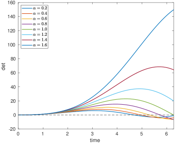
Figure 1: The determinant of the matrix $Y_{0}(t)$ for the circular orbits with period $T=2\pi$, for different values of $\alpha$.

For the case $\alpha=1$, a conjugate point appears exactly at the end point $T=2\pi$ of the time interval, hence the Jacobi condition (J) holds, but not the strengthened Jacobi condition (J’). Therefore, the gravitational Kepler problem provides an example where we can find global minimizers for which the sufficient conditions stated above for the weak local minimality are not satisfied, and the second variation is only non-negative definite. This is consistent with the result provided in [17], because the circular orbit is embedded in a family of periodic solutions of the Kepler problem with the same period. This degeneration is reflected in the fact that the second variation $\delta^{2}{\cal A}^{1}$ is only non-negative.

For the case $\alpha>1$ there are no conjugate points in $(0,T]$, hence the strengthened Jacobi condition (J’) holds for the second variation. The determinant of $Y_{0}(t)$ is greater than zero in $(0,T]$, and the dimension of the system is $n=2$, hence we are in the hypotheses of Lemma 3.12 and condition (SR) is therefore satisfied. It follows that the second variation of the circular orbit is positive definite, hence it is a (DLM). Moreover, the Lagrangian of the functional (5.3) comes from a mechanical system and it is globally convex in the velocity $\dot{u}$, hence by Remark 4.3 we know that the strengthened Weierstrass condition (W’) holds. Therefore, by Theorem 4.4 we are able to conclude that the circular orbit is a (SLM) on $X_{1}$. Note that this was expected, because we know that circular orbits are the global minimizers.

For $\alpha\in(0,1)$ a conjugate point appears inside the interval $(0,T)$ in the examples with $\alpha=0.2,\,0.4,\,0.6,\,0.8$. Hence circular solutions are not even local minimizers, but rather saddle points. This provides more information than what was proved in [34], where the author showed that the action of the circular orbit is greater than the action of the collision-ejection solution.

Computations for $k=2$.

As said above, finding the global minimizer of ${\cal A}^{\alpha}$ on $X_{k}$ is still an opened problem for $|k|\geq 2$. We provide here some computations for $k=2$ and $\alpha=1.2,1.3,1.4,1.5,1.6,1.7,1.8$. Figure 2 shows the determinant of $Y_{0}(t)$ relative to the circular orbit with period $2\pi$, in the time interval $[0,4\pi]$.

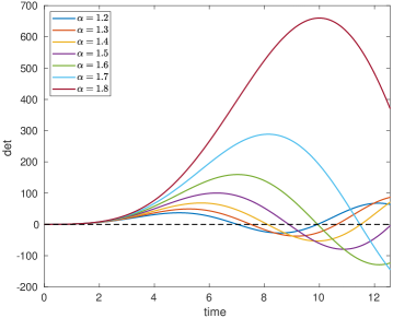
Figure 2: The determinant of the matrix $Y_{0}(t)$ for the circular orbits with period $2\pi$ in the time interval $[0,4\pi]$, for different values of $\alpha>1$.

We can notice that the circular solution has at least a conjugate point in $(0,4\pi)$ for $\alpha\leq 1.7$, hence the Jacobi condition (J) does not hold. Therefore it is not a minimizer anymore, but rather a saddle point.

To understand if a situation different from the case $k=1$ can occur, we can compare the action on $[0,4\pi]$ (that we denote with ${\cal A}^{\alpha}_{k},k=2$) of the circular solution $u_{0}$ with period $2\pi$, with the action of the collision-ejection solution $\bar{u}$. The action of the collision-ejection solution is

$${\cal A}^{\alpha}_{k}(\bar{u})=\bigg{(}\frac{2+\alpha}{2-\alpha}\bigg{)}(2\alpha^{2})^{-\frac{\alpha}{2+\alpha}}T^{\frac{2+\alpha}{2-\alpha}}\bigg{(}\int_{0}^{2\pi}|\sin t|^{2/\alpha}dt\bigg{)}^{\frac{2\alpha}{2+\alpha}},$$ (5.5)

while the action of a $k$-circular solution is

$${\cal A}^{\alpha}_{k}(u_{0})=k^{\frac{2\alpha}{2+\alpha}}(2+\alpha)\bigg{(}\frac{T}{2}\bigg{)}^{\frac{2+\alpha}{2-\alpha}}\bigg{(}\frac{\pi^{2}}{\alpha}\bigg{)}^{\frac{\alpha}{2+\alpha}},$$ (5.6)

see [34] for the details. Table 1 reports the values obtained from numerical evaluation of (5.5) and (5.6), for $T=4\pi$ and $k=2$.

$\alpha$	1.2	1.3	1.4	1.5	1.6	1.7	1.8
${\cal A}^{\alpha}_{2}(u_{0})$	18.777	18.698	18.599	18.483	18.355	18.218	18.073
${\cal A}^{\alpha}_{2}(\bar{u})$	12.585	13.286	14.349	15.974	18.563	23.057	32.281

Table 1: The value of the action ${\cal A}^{\alpha}_{2}$ of the circular solution $u_{0}$ with period $2\pi$ and of the collision-ejection solution $\bar{u}$.

Interestingly, we have that

$${\cal A}^{\alpha}_{2}(u_{0})<{\cal A}^{\alpha}_{2}(\bar{u})$$ (5.7)

for $\alpha=1.6,1.7,1.8$, meaning that the global minimizer is not a collision solution. On the other hand, for $\alpha=1.6,1.7$ the 2-circular solution $u_{0}$ is not a local minimizer because condition (J) does not hold, hence necessarily the global minimum is achieved by a non-collision and non-circular $T$-periodic solution. These simple examples already show that finding the global minimum of ${\cal A}^{\alpha}$ of $X_{k}$ for $\alpha\in(1,2)$ and $|k|\geq 2$ might be more complicated than the case of $k=\pm 1$.

5.2 The figure-eight solution of the 3-body problem

The figure-eight solution of the 3-body problem has been found first in [25] by using numerical methods. Later on, in [5] the authors were able to give a proof of the existence of such orbit by minimizing the action (1.1) over a particular set of loops. More accurate numerical studies were performed in [30, 29, 31], and the linear stability was finally proved by using rigorous numerical techniques in [22]. From the numerical point of view, the figure-eight solution is computed in two steps (see e.g. [11, 12] for details):

1. the action (1.1) is discretized by using truncated Fourier series, and a gradient descent method is applied to an eight-shaped first guess curve;

2. a shooting method is applied to the output of the gradient descent method, and an accurate initial condition is computed.

However, this procedure does not ensure that the final solution is actually a minimizer of the action. The initial conditions computed with this method are (see [5])

$$u_{1}=(0.97000435669734,-0.24308753153583),\quad u_{2}=-u_{1},\quad u_{3}=(0,0),$$

$$\dot{u}_{3}=(-0.93240737144104,-0.86473146092102),\quad\dot{u}_{1}=-\frac{\dot{u}_{3}}{2},\quad\dot{u}_{2}=-\frac{\dot{u}_{3}}{2},$$

while the period corresponds to $T\simeq 6.32591398292621$. The figure-eight solution also has a dihedral symmetry, meaning that it satisfies

$$\begin{cases}u_{1}(t+T/6)=Gu_{2}(t),\\ u_{2}(t+T/6)=Gu_{3}(t),\\ u_{3}(t+T/6)=Gu_{1}(t),\end{cases}\qquad G=\begin{pmatrix}-1&0\\ 0&1\\ \end{pmatrix},$$ (5.8)

and

$$\begin{cases}u_{1}(t)=u_{1}(-t),\\ u_{2}(t)=u_{3}(-t),\\ u_{3}(t)=u_{2}(-t).\end{cases}$$ (5.9)

Figure 3 shows the trajectory and the initial configurations of the masses, obtained by integrating the 3-body problem using the above initial conditions.

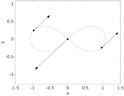
Figure 3: The trajectory and the initial configuration of the masses for the figure-eight solution of the 3-body problem.

By using a numerical integrator, we computed the solution $(Y_{0},Z_{0})$ of the Jacobi differential equation on the whole timespan $[0,T]$. The determinant of $Y_{0}$ is plotted as a function of the time in Figure 4.

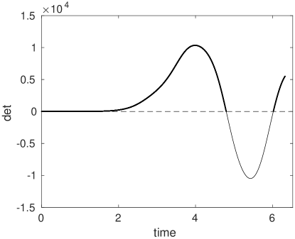
Figure 4: The determinant of $Y_{0}$ for the solution of the Jacobi differential equation corresponding to the figure-eight solution. The black thick curve corresponds to the intervals where $\det Y_{0}(t)>0$, while the thin black line corresponds to the interval where $\det Y_{0}(t)<0$.

A conjugate point appears, and therefore condition (J’) does not hold. This means that the figure-eight is not a local minimizer of the action on the whole set of $T$-periodic loops (note that this result was already found in [7]), but rather a saddle point.

It is worth stressing out that the proof of the existence of the figure-eight solution is made by proving that is minimizes the action (1.1). However, the set on which it is a minimizer is not the whole space of $T$-periodic planar loops, but rather on the subset $X$ of $T$-periodic loops fulfilling the symmetries (5.8) and (5.9). The theory presented in Section 3 and 4 is done by using the complete space of the $T$-periodic loops. This means that we also allow non-symmetric variations, that break the symmetry condition. For this reason, it is possible that we can choose a non-symmetric variation that reduces the value of the action, and this is not in contradiction with the figure-eight being a minimizer on the loop set $X$, that includes the symmetries. What we can do is to adapt the results of Section 3 and 4 by taking into the additional symmetry.

5.2.1 Including the symmetry in the theory

Here we include the symmetry in the space of loops. We are not going to present again the theory of local minimizers, but we underline the major changes to make in the conditions and the proofs. From now on, we always assume that condition (L’) holds. Let us suppose that the loops satisfy the condition

$$u\bigg{(}t+\frac{T}{M}\bigg{)}=Ru(t),\quad t\in[0,T],$$ (5.10)

where $R\in O(n)$ is a fixed orthogonal matrix and $M\in\mathbb{N}$ is an integer number. To make the discussion simpler, we suppose that $L$ does not depend on the time and

$$\int_{0}^{T}L(u,\dot{u})\,dt=M\int_{0}^{\frac{T}{M}}L(u,\dot{u})\,dt.$$ (5.11)

We therefore consider the functional

$$\mathcal{F}(\bar{u})=\int_{0}^{T/M}L(\bar{u},\dot{\bar{u}})\,dt,$$

defined on the set of loops $\bar{u}:[0,\,T/M]\to\mathbb{R}^{n}$ such that $R\bar{u}(0)=\bar{u}(T/M)$. Note that by means of (5.11), if $u_{0}:[0,T]\to\mathbb{R}^{n}$ is a minimizer of the functional ${\cal A}$, then the restriction

$$u_{0}\big{\lvert}_{[0,T/M]}:\bigg{[}0,\,\frac{T}{M}\bigg{]}\longrightarrow\mathbb{R}^{n},$$

is a minimizer of $\mathcal{F}$. Vice versa, if $\bar{u}_{0}:[0,T/M]\to\mathbb{R}^{n}$ is a minimizer of $\mathcal{F}$, then we can extend it to a closed loop $u_{0}:[0,T]\to\mathbb{R}^{n}$ by using the symmetry (5.10), and we obtain a minimizer for ${\cal A}$. Therefore, we study the minimality of $u_{0}$ restricted to the interval $[0,T/M]$ as stationary point of the functional $\mathcal{F}$.

To understand what is the equivalent condition of the (SR) condition, we follow the steps of the proof of Theorem 3.11. We still write the quadratic functional using a symmetric solution $W$ defined on $[0,T/M]$ and, integrating by parts, the term outside the integral becomes

$$\begin{split}v(t)\cdot W(t)v(t)\bigg{|}_{0}^{T/M}&=v(T/M)\cdot W(T/M)v(T/M)-v(0)\cdot W(0)v(0)\\ &=v(0)\cdot\bigg{(}R^{T}W(T/M)R-W(0)\bigg{)}v(0).\end{split}$$

Therefore, a symmetric solution $W$ of the Riccati differential equation satisfying the boundary condition

$$R^{T}W(T/M)R-W(0)>0,$$ (5.12)

is sufficient to ensure the positivity of a quadratic functional. (SR) condition is then replaced by (SR*), i.e. there exists a symmetric solution $W$ of the (RDE) defined on the whole $[0,T/M]$ such that (5.12) holds.

The equivalent of Lemma 3.12 is obtained by replacing $T$ with $T/M$ and (SR) with (SR*). The proof remains the same if we notice that the map $w\mapsto Rw$ is invertible and maps the unit sphere onto itself.

Regarding the weak and the strong local minimality, the proof of Theorem 4.4 remains the same if we assume that

$$p(0)-R^{T}p\bigg{(}\frac{T}{M}\bigg{)}=0,$$ (5.13)

where $p(t)=L_{\dot{u}}(t,u_{0}(t),\dot{u}_{0}(t))$. Note that if the derivative $L_{\dot{u}}$ is such that

$$L_{\dot{u}}(Ru,Rv)=RL_{\dot{u}}(u,v),$$ (5.14)

for all $(u,v)$, then condition (5.13) is verified, and the remaining part of the proof of Theorem 4.4 is the same.

Implications for the figure-eight orbit.

Denoting with $O_{2}$ the $2\times 2$ matrix containing only zeros, and setting

$$R=\begin{pmatrix}O_{2}&G&O_{2}\\ O_{2}&O_{2}&G\\ G&O_{2}&O_{2}\end{pmatrix}\in O(6),$$ (5.15)

the symmetry (5.8) of the figure-eight can be written as $u(t+T/6)=Ru(t)$, where $u(t)=\big{(}u_{1}(t),u_{2}(t),u_{3}(t)\big{)}\in\mathbb{R}^{6}$. From Figure 4, we can see that the determinant of $Y_{0}(t)$ is positive in the whole interval $[0,T/6]$. Since the orbit is planar, the dimension $n=6$ of the system is even, and by applying the corresponding version of Lemma 3.12 we find that condition (SR*) holds. Therefore, by the corresponding version of Theorem 3.11 the figure-eight solution is a (DLM) over the space $X$ of $T$-periodic loops satisfying the symmetry condition (5.8).

Moreover, condition (5.14) is trivially satisfied for the Lagrangian of the $N$-body problem, and the Weierstrass condition (W’) holds because of Remark 4.3. Therefore, we can apply the corresponding version of Theorem 4.4, finding that the figure-eight solution is a (SLM) on the same set of symmetric loops $X$.

Data availability statement

The datasets generated during and/or analysed during the current study are available from the corresponding author on reasonable request.

References

- [1] J. Allwright and R. Vinter. Second order conditions for periodic optimal control problems. Control Cybernet., 34(3):617–643, 2005.
- [2] E. Barrabés, J. M. Cors, C. Pinyol, and J. Soler. Hip-hop solutions of the -body problem. Celestial Mechanics and Dynamical Astronomy, 95(1):5–66, May 2006.
- [3] A. Chenciner. Action minimizing solutions of the newtonian -body problem: from homology to symmetry. In Proceedings of the International Congress of Mathematicians, Vol. III (Beijing, 2002), pages 279–294. Higher Ed. Press, Beijing, 2002.
- [4] A. Chenciner. Symmetries and “simple” solutions of the classical -body problem. In XIVth International Congress on Mathematical Physics, pages 4–20. World Sci. Publ., Hackensack, NJ, 2005.
- [5] A. Chenciner and R. Montgomery. A remarkable periodic solution of the three-body problem in the case of equal masses. Annals of Mathematics, 152(3):881–901, 2000.
- [6] A. Chenciner and A. Venturelli. Minima de l’intégrale d’action du problème newtonien de 4 corps de masses égales dans : orbites “hip-hop”. Cel. Mech. Dyn. Ast., 77(2):139–152, 2000.
- [7] N. N. Chtcherbakova. On the minimizing properties of the 8-shaped solution of the 3-body problem. Journal of Mathematical Sciences, 135(4):3256–3268, 2006.
- [8] F. H. Clarke and V. Zeidan. Sufficiency and the Jacobi condition in the calculus of variations. Canad. J. Math., 38(5):1199–1209, 1986.
- [9] Z. Došlá and O. Došlý. Quadratic functionals with general boundary conditions. Appl. Math. Optim., 36(3):243–262, 1997.
- [10] Z. Došlá and P. Zezza. Conjugate points in the calculus of variations and optimal control theory via the quadratic form theory. Differential Equations Dynam. Systems, 2:137–152, 01 1994.
- [11] M. Fenucci and G. F. Gronchi. On the stability of periodic -body motions with the symmetry of Platonic polyhedra. Nonlinearity, 31(11):4935, 2018.
- [12] M. Fenucci and À Jorba. Braids with the symmetries of Platonic polyhedra in the Coulomb (N+1)-body problem. Communications in Nonlinear Science and Numerical Simulation, 83:105105, 2020.
- [13] D. L. Ferrario and S. Terracini. On the existence of collisionless equivariant minimizers for the classical -body problem. Inventiones mathematicae, 155(2):305–362, 2004.
- [14] G. Fusco, G. F. Gronchi, and P. Negrini. Platonic polyhedra, topological constraints and periodic solutions of the classical -body problem. Inventiones mathematicae, 185(2):283–332, 2011.
- [15] M. Giaquinta and S. Hildebrandt. Calculus of Variations I. Grundlehren der mathematischen Wissenschaften. Springer Berlin Heidelberg, 2004.
- [16] H. H. Goldstine. A History of the Calculus of Variations from the 17th through the 19th Century. Studies in the History of Mathematics and Physical Sciences 5. Springer-Verlag New York, 1 edition, 1980.
- [17] W. B. Gordon. A minimizing property of Keplerian orbits. Amer. J. Math., 99(5):961–971, 1977.
- [18] L. Haws and T. Kiser. Exploring the brachistochrone problem. The American Mathematical Monthly, 102(4):328–336, 1995.
- [19] M.R. Hestenes. Calculus of Variations and Optimal Control Theory. Applied mathematics series. John Wiley & Sons, 1966.
- [20] R. Hilscher and V. Zeidan. Applications of time scale symplectic systems without normality. J. Math. Anal. Appl., 340(1):451–465, 2008.
- [21] R. Hilscher and V. Zeidan. Riccati equations for abnormal time scale quadratic functionals. J. Differential Equations, 244(6):1410–1447, 2008.
- [22] T. Kapela and C. Simó. Computer assisted proofs for nonsymmetric planar choreographies and for stability of the eight. Nonlinearity, 20:1241–1255, 2007.
- [23] T. Kapela and C. Simó. Rigorous KAM results around arbitrary periodic orbits for Hamiltonian systems. Nonlinearity, 30(3):965–986, 2017.
- [24] T. Kapela and P. Zgliczynski. The existence of simple choreographies for the -body problem - a computer assisted proof. Nonlinearity, 16(6):1899–1918, 2003.
- [25] C. Moore. Braids in classical dynamics. Phys. Rev. Lett., 70(24):3675–3679, 1993.
- [26] C. Moore and M. Nauenberg. New periodic orbits for the -body problem. Journal of Computational and Nonlinear Dynamics, 1(4):307–311, 2006.
- [27] L.A. Pars. An introduction to the calculus of variations. Wiley, 1962.
- [28] J. P. Phillips. Brachistochrone, tautochrone, cycloid—apple of discord. The Mathematics Teacher, 60(5):506–508, 1967.
- [29] C. Simó. New families of solutions in -body problems. In Carles Casacuberta, Rosa Maria Miró-Roig, Joan Verdera, and Sebastià Xambó-Descamps, editors, European Congress of Mathematics: Barcelona, July 10–14, 2000, Volume I, pages 101–115, Basel, 2001. Birkhäuser Basel.
- [30] C. Simó. Periodic orbits of the planar -body problem with equal masses and all bodies on the same path, pages 265–284. IoP Publishing, 2001.
- [31] C. Simó. Dynamical properties of the figure eight solution of the three-body problem. In Celestial mechanics (Evanston, IL, 1999), volume 292 of Contemp. Math., pages 209–228. Amer. Math. Soc., Providence, RI, 2002.
- [32] G. Stefani and P. Zezza. Constrained regular LQ-control problems. SIAM J. Control Optim., 35(3):876–900, 1997.
- [33] B. van Brunt. The Calculus of Variations. Universitext. Springer New York, 2003.
- [34] A. Venturelli. Application de la minimisation de l’action au Problème de N corps dans le plan e dans l’espace. PhD thesis, University of Paris VII, 2002.
- [35] V. Zeidan. Sufficiency criteria via focal points and via coupled points. SIAM Journal on Control and Optimization, 30(1):82–98, 1992.
- [36] V. Zeidan. Sufficient conditions for variational problems with variable endpoints: Coupled points. Applied Mathematics and Optimization, 27(2):191–209, 1993.
- [37] V. Zeidan. Nonnegativity and positivity of a quadratic functional. Dynam. Systems Appl., 8(3-4):571–588, 1999.
- [38] V. Zeidan. New second-order optimality conditions for variational problems with -Hamiltonians. SIAM Journal on Control and Optimization, 40(2):577–609, 2001.
- [39] V. Zeidan and P. Zezza. Coupled points in the calculus of variations and applications to periodic problems. Trans. Amer. Math. Soc., 315(1):323–335, 1989.