Semi-global Periodic Event-triggered Output Regulation for Nonlinear Multi-agent Systems

Abstract

This study focuses on periodic event-triggered (PET) cooperative output regulation problem for a class of nonlinear multi-agent systems. The key feature of PET mechanism is that event-triggered conditions are required to be monitored only periodically. This approach is beneficial for Zeno behavior exclusion and saving of battery energy of onboard sensors. At first, new PET distributed observers are proposed to estimate the leader information. We show that the estimation error converges to zero exponentially with a known convergence rate under asynchronous PET communication. Second, a novel PET output feedback controller is designed for the underlying strict feedback nonlinear multi-agent systems. Based on a state transformation technique and a local PET state observer, the cooperative semi-global output regulation problem can be solved by the proposed new control design technique. Simulation results of multiple Lorenz systems illustrate that the developed control scheme is effective.

I Introduction

Output regulation problem has attracted an increasing attention recently. Output regulation aims to make tracking error converge to zero while rejecting disturbance. Reference and disturbance signals are produced by an exosystem. For typical examples, the internal model principle was used for the output regulation of linear multi-variable systems [1]. [2, 3, 4] focused on the output regulation problem of nonlinear systems. Different classes of nonlinear systems, such as first order system, output feedback system and strict feedback system, were considered.

The output regulation theory has also been shown to be a powerful method for multi-agent systems [5, 6, 7, 8, 9]. On the basis of this theory, the leader-following problem can be handled effectively despite parametric uncertainties and external disturbance. For instance, in [10, 11], the cooperative output regulation problem for linear and nonlinear multi-agent systems were solved using distributed observer technique.

With the continuous development of embedded microprocessors in engineering system, a critical issue for multi-agent systems is reducing the communication burden. Apparently, continuous communication may be unrealistic in most applications because the bandwidth and energy are limited. Event-triggered control strategy has been lately introduced for the cooperative control of multi-agent systems [12, 13]. The idea of the event-triggered control is that data transmission is conducted only under some certain conditions. Event-triggered mechanism is an effective method for resource-limited applications. A number of works on various kinds of event-triggered control methods [14, 15, 16] have been conducted.

More recently, in [17, 18], a new periodic event-triggered (PET) control method has been presented. Different from other event-triggered mechanisms, PET mechanism is required to monitor data communication and triggered conditions only at discrete sampling instants. This characteristic brings some promising advantages (see [24]). First, the inter-event time naturally becomes multiples of sampling periods. This condition not only strictly excludes the Zeno behavior but is also useful for digital implementation where tasks are always executed periodically. Second, the energy for evaluating the event-triggered condition can also be saved given that no continuous monitoring exists. This condition is beneficial for saving the battery energy of onboard sensors. However, to the best of our knowledge, the PET cooperative output regulation problem for nonlinear multi-agent systems has not been fully investigated.

Inspired by the above observation, in this paper we investigate the problem of PET cooperative output regulation for a class of nonlinear multi-agent systems. The main challenges are as follows:

1) The communication of multi-agent systems is assumed to be asynchronous. That is, each agent may have different sampling times and transmit data asynchronously. Thus, the existing distributed observers [11, 19, 20] become invalid;

2) Each agent is described by a high order strict feedback nonlinear system. Moreover, only the output information of each agent is available. This setup is more general than the existing works [11, 21, 22] (see Remark 2); and

3) Note that the sampled data control can be regarded as a special case of the PET control. However, very few works have been conducted on sampled data output regulation for nonlinear systems, not to mention the PET control. In fact, only recently, the PET/sampled data output regulation problem has been solved for linear systems [23, 24]. The nonlinear dynamics of the considered systems will cause many difficulties to the PET output regulation problem.

To overcome the these difficulties, we provide our main contributions as follows:

• New PET distributed observers are proposed to estimate the leader information. On the basis of the properties of time-delay systems, exponential functions and matrix norms, we demonstrate that the estimation error will converge to zero exponentially with a known convergence rate under asynchronous PET communication.

• A novel PET output feedback controller is presented for the strict feedback nonlinear multi-agent systems. Based on a state transformation technique and a local PET observer, we show that the proposed PET output feedback controller can solve the cooperative semi-global output regulation problem. Lyapunov function in logarithm form and Gronwall’s inequality are skillfully used to prove this result.

This paper is organized as follows. Section II presents problem formulation and preliminaries. New PET distributed observer and PET control law are provided in Sections III and IV respectively. In Section V simulation results of multiple Lorenz systems are presented to demonstrate the effectiveness of the proposed new design scheme. The conclusion is drawn in Section VI. Detailed proofs are put in the Appendices.

Notations. For a matrix $X_{i}\in\mathbb{R}^{n_{i}\times m}(i=1,2,...,N)$, $\mathrm{col}(X_{1},X_{2},...,X_{N})=[X_{1}^{\mathrm{T}}\thinspace X_{2}^{\mathrm{T}}\thinspace...X_{N}^{\mathrm{T}}]^{\mathrm{T}}$. For $A\in\mathbb{R}^{n\times m}$, $\mathrm{vec}(A)=\mathrm{col}(a_{1},...,a_{n})$ where $a_{i}\in\mathbb{R}^{n\times 1}$ is the $i$th column of $A$. $\mathrm{sat_{\mathit{R}}}(x):\mathbb{R}\rightarrow\mathbb{R}$ with a positive constant $R$ represents the saturation function, that is $\mathrm{sat_{\mathit{R}}}(x)=x$ if $|x|\leq R$, $\mathrm{sat_{\mathit{R}}}(x)=R$ if $x>R$ and $\mathrm{sat_{\mathit{R}}}(x)=-R$ if $x<-R$. Given a time-varying matrix $B(t)\in\mathbb{R}^{n\times m}$, define a set $\mathsf{E}(\gamma)$ with a positive constant $\gamma$. If $B(t)\in\mathsf{E}(\gamma)$ then $||B(t)||$ converges to zero exponentially, that is, $||B||\leq c\mathrm{e}^{-\gamma t}$ for $\forall t\in[0,+\infty)$ where $c$ is a positive constant.

II Problem formulation and preliminaries

II-A Problem formulation

The following multi-agent systems consisting of one leader and $N$ followers are considered. The leader is expressed as:

$$\dot{\nu} =A\nu,$$ (1)

$${\color[rgb]{0,0,0}y_{0}} {\color[rgb]{0,0,0}=q_{0}(\nu)}$$ (2)

where $\nu\in\mathbb{R}^{n_{\nu}}$ is the reference signal and/or external disturbance with $n_{\nu}\in\mathbb{N}$. $y_{0}\in\mathbb{R}$ is the output of the leader. $A$ is a given system matrix, $q_{0}(\nu)$ is a sufficiently smooth function with ${\color[rgb]{0,0,0}q_{0}(0)=0}$. Meanwhile, assume that there exists a known compact set $\mathbb{V}\subseteq\mathbb{R}^{n_{\nu}}$ such that $\nu\in\mathbb{V}$.

The followers are given by strict feedback nonlinear systems:

$$\dot{z}_{i} =f_{i0}(z_{i},x_{i1},\nu,w),$$

$$\dot{x}_{ij} =f_{ij}(z_{i},x_{i1},...,x_{ij},\nu,w)+b_{ij}(w)x_{i,j+1},$$

$$\dot{x}_{in} =f_{in}(z_{i},x_{i1},...,x_{in},\nu,w)+b_{in}(w)u_{i},$$ (3)

$$y_{i} =x_{i1},\thinspace j=1,2,...,n-1$$

where $i\in\{1,2,...,N\}$. $n\in\mathbb{N}$ is the order of the $i$th subsystem, $z_{i}\in\mathbb{R}^{n_{z_{i}}}$ and $x_{ij},x_{in}\in\mathbb{R}$ denote the system states with $n_{z_{i}}\in\mathbb{N}$, $y_{i}\in\mathbb{R}$ is the system output. $w\in\mathbb{R}^{n_{w}}$ represents uncertain parameters with $n_{w}\in\mathbb{N}$. Also assume that there exists a known compact set $\mathbb{W}\subseteq\mathbb{R}^{n_{w}}$ such that $w\in\mathbb{W}$. $f_{i0}(\cdot),f_{ij}(\cdot),b_{ij}(w)(i=1,...,N;j=1,...,n)$ are sufficiently smooth nonlinear functions with $f_{i0}(0,...,0,w)=0,f_{ij}(0,...,0,w)=0$ and $b_{ij}(w)>0$ for $\forall w\in\mathbb{W}$.

A directed graph $\mathcal{G}$ is used to describe the communication for the multi-agent systems. Let $\mathcal{G}=(\mathcal{V},\mathcal{E})$ where $\mathcal{V}=\{1,2,...,N\}$ denotes the set of vertices and $\mathcal{E}\subseteq\mathcal{V}\times\mathcal{V}$ represents the set of edges. Matrix $\widetilde{A}=[a_{ij}]\in\mathbb{R}^{N\times N}$ is defined, such that if $(j,i)\in\mathcal{E}$ then $a_{ij}=1$, otherwise $a_{ij}=0$. Laplacian matrix is defined as $\mathcal{L}=\widetilde{D}-\widetilde{A}$ with $\widetilde{D}=\mathrm{diag}(\tilde{d}_{1},\tilde{d}_{2},...,\tilde{d}_{N})$ and $\tilde{d}_{i}=\sum_{j=1}^{N}a_{ij}(i\in\mathcal{V})$. For communication between the leader and followers, $a_{i0}$ is defined such that if the followers can have access to the leader, then $a_{i0}=1$; otherwise $a_{i0}=0$. This indicates that only a small number of followers can obtain the information of the leader. Finally, we assume that there exists a directed spanning tree for the considered graph with the leader as the root. Then, we know $-\mathcal{H}=-(\mathcal{L}+\widetilde{B})$ is Hurwitz with $\widetilde{B}=\mathrm{diag}(a_{10},a_{20},...,a_{N0}).$

The problem we are going to solve is formulated as follows:

Problem 1.

(Cooperative semi-global output regulation problem) Consider the multi-agent systems (1)-(3) with their corresponding graph $\mathcal{G}$. Suppose that the initial states $\nu(0),z_{i}(0),x_{ij}(0)$ of the systems belong to a given compact set. The control objective is to design a PET distributed output feedback control law for each follower such that

1) All the signals are uniformly bounded for $\forall t\in[0,+\infty)$; and,

2) The output regulation error $e_{i}(t)\triangleq y_{i}(t)-y_{0}(t)$ converges to zero exponentially, $i.e.$, $\underset{t\rightarrow+\infty}{\lim}|e_{i}(t)|\rightarrow 0$ $\forall i\in\{1,2,...,N\}$.

Remark 1.

The signals in Problem 1 are all the signals in the closed-loop control system. They include all the states $x_{ij}(i=1,...,n;j=1,...N)$ of the followers, the control input $u_{i}$, the variables $\hat{\nu}_{i},\hat{\xi}_{i}$ in the proposed distributed observer and state observer in Sections III-IV $etc$.

Remark 2.

Contrary to the existing works, the considered problem is more general and practical. The reasons are as follows:

1) System (3) is in a high order strict feedback form. The strict feedback nonlinear systems is more general than many other kinds of nonlinear systems [11, 19, 22, 25], such as linear systems, low order nonlinear systems, normal form nonlinear systems $etc$.

2) Different from [20, 21] that deals with state feedback control, we consider output feedback control problem for nonlinear systems. The problem becomes more involved because only output information of the high order nonlinear system (3) is available.

3) The PET data transmission is considered. This means that only PET output information is available for the controller design, which will further complicate the design and analysis process.

4) The output regulation problem is examined, where reference tracking, disturbance rejection and parametric uncertainties are simultaneously considered. Our study extends the results in [26, 27], where only reference tracking problem is studied.

II-B Preliminaries

We introduce some basic assumptions and useful results.

1) Leader

For the leader dynamic of (1), assume

Assumption 1.

$A$ in (1) is a skew-symmetric matrix whose eigenvalues are semi-simple with zero real parts.

Remark 3.

Assumption 1 is standard in output regulation problem [3, 20]. When $A$ is neutrally stable, a large class of commonly used signals $\nu$, such as sine, cosine and constant signals, can be produced.

2) Followers

For the nonlinear system (3), we have:

Assumption 2.

$f_{i0}(\mathbf{z}_{i}(\nu,w),q_{0}(\nu),\nu,w)(i=1,2,...,N)$ satisfies

$$\frac{\partial\mathbf{z}_{i}(\nu,w)}{\partial\nu}A\nu=f_{i0}(\mathbf{z}_{i}(\nu,w),q_{0}(\nu),\nu,w)$$

where $\mathbf{z}_{i}(\nu,w)$ is a smooth function with $\mathbf{z}_{i}(0,0)=0$.

Meanwhile, under Assumption 2, one can compute the solution to the regulator equation related to (1) and (3) (see [3, 21]). The solution is given by:

$$\mathbf{x}_{i1}(\nu)=q_{0}(\nu),$$

$$\mathbf{x}_{i,j+1}(\nu,w)$$

$$= b_{ij}^{-1}(w)\left(\frac{\partial\mathbf{x}_{ij}}{\partial\nu}A\nu-f_{ij}(\mathbf{z}_{i},\mathbf{x}_{i1},...,\mathbf{x}_{ij},\nu,w)\right),$$

$$\mathbf{u}_{i}(\nu,w)=b_{in}^{-1}(w)\left(\frac{\partial\mathbf{x}_{in}}{\partial\nu}A\nu-f_{in}(\mathbf{z}_{i},\mathbf{x}_{i1},...,\mathbf{x}_{in},\nu,w)\right)$$

where $j=1,2,...,n-1$. In addition, define $\mathbf{x}_{i,n+1}(\nu,w)\triangleq\mathbf{u}_{i}(\nu,w)$.

We also make the following standard assumption for $\mathbf{x}_{i1}(\nu),\mathbf{x}_{i,j+1}(\nu,w)(j=1,2,...,n)$.

Assumption 3.

Assume that $\mathbf{x}_{i1}(\nu),\mathbf{x}_{i,j+1}(\nu,w)(j=1,2,...,n)$ are all polynomials in $\nu$ with coefficients depending on $w$.

Remark 4.

If the considered system (3) is in a polynomial form, Assumption 3 will hold according to [25]. Assumption 3 guarantees the solvability of the output regulation problem.

By resorting to [3, 21], Assumption 3 indicates that for any $\nu\in\mathbb{V},w\in\mathbb{W},j=1,2,...,n$, we have

$$\frac{d^{\overline{n}_{ij}}\mathbf{x}_{i,j+1}}{dt^{\overline{n}_{ij}}}=\lambda_{i1}\mathbf{x}_{i,j+1}+\lambda_{i2}\frac{d\mathbf{x}_{i,j+1}}{dt}+\cdots+\lambda_{i\overline{n}_{ij}}\frac{d^{(\overline{n}_{ij}-1)}\mathbf{x}_{i,j+1}}{dt^{(\overline{n}_{ij}-1)}}$$

where $\overline{n}_{ij}\in\mathbb{N}$. $\lambda_{i1},...,\lambda_{i\overline{n}_{ij}}$ are real constants such that the roots of the polynomial $p_{ij}(s)=s^{\overline{n}_{ij}}-\lambda_{i1}-\lambda_{i2}s-\cdots-\lambda_{i\overline{n}_{ij}}s^{\overline{n}_{ij}-1}$ are distinct with zero real parts.

Then, given any column vector $N_{ij}\in\mathbb{R}^{\overline{n}_{ij}}$ and Hurwitz matrix $M_{ij}$ satisfying $(M_{ij},N_{ij})$ are controllable, we have

$$T_{ij}\Psi_{ij}-M_{ij}T_{ij}=N_{ij}\Gamma_{ij}$$

where $T_{ij}$ is a nonsingular matrix. $\Gamma_{ij}=[1\thinspace 0\thinspace...\thinspace 0],$

$$\Psi_{ij}=\left[\begin{array}[]{cccc}&1\\ &&\ddots\\ &&&1\\ \lambda_{i1}&\lambda_{i2}&\cdots&\lambda_{i\overline{n}_{ij}}\end{array}\right].$$

Let $\theta_{ij}(\nu,w)=T_{ij}\mathrm{col}(\mathbf{x}_{i,j+1},\frac{d\mathbf{x}_{i,j+1}}{dt},...,\frac{d^{(\overline{n}_{ij}-1)}\mathbf{x}_{i,j+1}}{dt^{(\overline{n}_{ij}-1)}})$. Thus, we obtain:

$$\dot{\theta}_{ij}(\nu,w)= T_{ij}\Psi_{ij}T_{ij}^{-1}\theta_{ij}(\nu,w),$$

$${\color[rgb]{0,0,0}\mathbf{x}_{i,j+1}(\nu,w)}= {\color[rgb]{0,0,0}\Phi_{ij}\theta_{ij}(\nu,w)}$$ (4)

where $\Phi_{ij}=\Gamma_{ij}T_{ij}^{-1}.$

It can be seen that (4) generates the steady state $\mathbf{x}_{i,j+1}(\nu,w)$. Then we can design the following dynamic compensator:

$$\dot{\eta}_{ij} =M_{ij}\eta_{ij}+N_{ij}x_{i,j+1},$$

$$\dot{\eta}_{in} =M_{in}\eta_{in}+N_{in}u_{i}$$ (5)

where $\eta_{ij},\eta_{in}$ are dynamic variables and $j=1,2,...,n-1$.

(5) is also called the internal model for system (1) and (3). It plays a pivotal role in solving the output regulation problem.

Finally, the following change of coordinates is considered for system (3):

$$\overline{z}_{i} =z_{i}-\mathbf{z}_{i}(\nu,w),$$

$$\overline{x}_{i1} =x_{i1}-\mathbf{x}_{i1}(\nu),$$

$${\color[rgb]{0,0,0}\overline{x}_{ij}} {\color[rgb]{0,0,0}=x_{ij}-\Psi_{i,j-1}\eta_{i,j-1}\thinspace(j=2,...,n),}$$

$${\color[rgb]{0,0,0}{\color[rgb]{0,0,0}\tilde{\eta}_{ij}}} {\color[rgb]{0,0,0}{\color[rgb]{0,0,0}=\eta_{ij}-\theta_{ij}(\nu,w)-b_{ij}^{-1}(w)N_{ij}\overline{x}_{ij}}\thinspace(j=1,...,n),}$$ (6)

$$\overline{x}_{i,n+1} \triangleq\overline{u}_{i}=u_{i}-\Psi_{in}\eta_{in}.$$ (7)

Then, systems (1) and (3) can be written as:

$$\dot{\overline{z}}_{i} =\overline{f}_{i0}(\overline{z}_{i},\overline{x}_{1i},\nu,w),$$

$$\dot{\tilde{\eta}}_{ij} =M_{ij}\tilde{\eta}_{ij}+g_{ij}(\overline{z}_{i},\tilde{\eta}_{i1},...,\tilde{\eta}_{i,j-1},\overline{x}_{i1},...,\overline{x}_{ij},\nu,w),$$

$$\dot{\overline{x}}_{ij} =\overline{f}_{ij}(\overline{z}_{i},\tilde{\eta}_{i1},...,\tilde{\eta}_{ij},\overline{x}_{i1},...,\overline{x}_{ij},\nu,w)+b_{ij}(w)\overline{x}_{i,j+1},$$

$$e_{i} =\overline{x}_{i1},\thinspace i=1,2,...,N;\thinspace j=1,2,...,n$$ (8)

where $\overline{f}_{i0}(\cdot),g_{ij}(\cdot),\overline{f}_{ij}(\cdot)(i=1,...,N;j=1,...,n)$ are sufficiently smooth nonlinear functions with $\overline{f}_{i0}(0,...,0,\nu,w)=0,g_{ij}(0,...,0,\nu,w)=0,\overline{f}_{ij}(0,...,0,\nu,w)=0$ for $\forall\nu\in\mathbb{V},\forall w\in\mathbb{W}$.

It is noted that according to the above change of coordinates, the output regulation problem is transformed into the stabilization problem. Namely, if one can stabilize system (8), $i.e.$, find a controller $u_{i}$ to make $\overline{x}_{ij}(t)\rightarrow 0(i=1,...,N;j=1,...,n)$ as $t\rightarrow+\infty$, then the error $e_{i}$ will be regulated to zero. Therefore, in the following we will mainly consider the stabilization problem of system (8).

For the $\overline{z}_{i}$-system, we make the following assumption.

Assumption 4.

[22, 28] Assume that there exists a $C^{2}$ positive definite Lyapunov function $V_{i0}(\overline{z}_{i})$ such that

$$\frac{\partial V_{i0}(\overline{z}_{i})}{\partial\overline{z}_{i}}\overline{f}_{i0}(\overline{z}_{i},0,\nu,w)\leq-\gamma_{i0}||\overline{z}_{i}||^{2}$$

where $\gamma_{i0}$ is a known positive constant.

Remark 5.

The $z_{i}$-subsystem represents the dynamic uncertainty/unmodeled dynamics of the system. The states of the $z_{i}$-subsystem may not be available for feedback control. Assumption 4 means that the zero dynamic of the $z_{i}$-system is asymptotically stable. It is less conservative than the assumption of input-to-state stability in [25]. As a result, it is possible to find a control law that does not rely on the states of the $z_{i}$-subsystem. A lot of real practical systems satisfy Assumptions 3 and 4, such as Lorenz system, Chua’s circuit, servo motors and robot mainpulators.

3) Useful results

We present some properties of matrix norms and useful inequalities.

Lemma 1.

1) (Property of skew-symmetric matrix) Given any skew-symmetric matrix $A\in\mathbb{R}^{n\times n}$ and matrix $B\in\mathbb{R}^{n\times m}$, we have $||\mathrm{e}^{A}||=1$ and $||\mathrm{e}^{A}B||=||B||$;

2) [29] For some square matrices $A,B\in\mathbb{R}^{n\times n}$, $||\mathrm{e}^{A}-\mathrm{e}^{B}||\leq\mathrm{e}^{||A||+||B-A||}||B-A||$;

3) (Gronwall’s inequality) Suppose

$$u(t)\leq\rho_{1}+\int_{t_{0}}^{t}\rho_{2}u(\tau)d\tau$$

for $\forall t\in[t_{0},+\infty)$ where $u(t):[t_{0},+\infty)\rightarrow\mathbb{R}$ is a time-varying function, $\rho_{1},\rho_{2},t_{0}>0$ are positive constants. Then, $u(t)\leq\rho_{1}\mathrm{e}^{\rho_{2}(t-t_{0})}$;

4) [30] Given $u,u^{*}\in\mathbb{R}$ with $u\in[-R,R]$, then $|u-\mathrm{sat}_{R}(u^{*})|\leq\min\{|u-u^{*}|,2R\}$ where $R$ is a positive constant.

III PET distributed observer

The proposed controller structure is illustrated in Fig. 1 (The switch is on node 1. Section IV-D will discuss the case when the switch is on node 2). It is composed of a PET distributed observer and a PET control law. The PET distributed observer is implemented in the sensor side to estimate the leader information. The control law uses estimated information to generate control signal. PET mechanisms are used for communications between each connected agent pair and the sensor-to-controller transmission channel in each agent.

Next, we will explain the PET distributed observer in this section, where two different cases are considered. The control law will be explained in the next section.

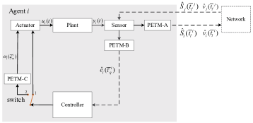
Figure 1: Event-triggered control scheme.

III-A Case one

In this case, we assume that only a small number of the followers know the information $\nu$ of the leader. That is, only followers connected to the leader have access to $\nu$ (For instance, in Fig. 2, among the four followers only agent 1 know $\nu$). Meanwhile, the matrix $A$ of the leader is known to all the followers. We design the following distributed observer for agent $i(i=1,2,...,N)$.

$$\dot{\hat{\nu}}_{i} =A\hat{\nu}_{i}+\mu_{2}\sum_{j=0}^{N}a_{ij}(\overline{\nu}_{j}(t,\overline{t}_{l^{\prime}}^{j})-\overline{\nu}_{i}(t,\overline{t}_{l}^{i}))$$ (9)

where $\hat{\nu}_{i}$ is used to estimate the leader information $\nu$,

$$\overline{\nu}_{i}(t,\overline{t}_{l}^{i})=\mathrm{e}^{A(t-\overline{t}_{l}^{i})}\hat{\nu}_{i}(\overline{t}_{l}^{i})(i=1,...,N)$$ (10)

with $\hat{\nu}_{0}\triangleq\nu$, $\overline{\nu}_{0}(t,t_{l}^{0})=\mathrm{e}^{A(t-t_{l}^{0})}\hat{\nu}_{0}(t_{l}^{0})=\mathrm{e}^{A(t-t_{l}^{0})}\nu(t_{l}^{0})=\nu(t)$. $\mu_{2}>0$ is a positive parameter.

The above distributed observer (9) runs with respect to the time $t\in[0,+\infty)$. Next, we will explain the time instants $\overline{t}_{l}^{i}$ and $\overline{t}_{l^{\prime}}^{j}$. Let $0=t_{0}^{i}<t_{1}^{i}<\cdots<t_{k}^{i}<\cdots$ denote the sampling time instants for agent $i$ where $t_{k}^{i}\triangleq kT^{i}$ and $T^{i}>0$ represents the sampling period. Let $T\triangleq\underset{i\in\{1,2,...,N\}}{\max}T^{i}$ and define set $\Omega_{T}^{i}=\{t_{0}^{i},t_{1}^{i},...,t_{k}^{i},...\}.$ With slight abuse of notation, we use $t_{k}^{i}$ and $t_{k^{\prime}}^{j}$ denote the latest sampling time instants for agent $i$ and $j$ at the current time $t$.

Then, let $0=\overline{t}_{0}^{i}<\overline{t}_{1}^{i}<\cdots<\overline{t}_{l}^{i}<\cdots$ denote the event-triggered time instants. On time instant $\overline{t}_{l}^{i}$, agent $i$ will send $\hat{\nu}_{i}(\overline{t}_{l}^{i})$ to its neighbors. $\overline{t}_{l}^{i}$ is determined by the Periodic Event-Triggered Mechanism A (PETM-A) in Fig. 1, that is

$$\overline{t}_{l+1}^{i}=\mathrm{inf}\{\tau>\overline{t}_{l}^{i}|\tau\in\Omega_{T}^{i},h_{\nu}^{i}(\tau,\overline{t}_{l}^{i})>0\}$$ (11)

where

$$h_{\nu}^{i}(\tau,\overline{t}_{l}^{i})=||\hat{\nu}_{i}(\tau)-\overline{\nu}_{i}(\tau,\overline{t}_{l}^{i})||-\iota_{\nu}\mathrm{e}^{-\gamma_{\nu}\tau}$$

with positive constants $\iota_{\nu},\gamma_{\nu}>0$.

It can be seen that the set $\Omega_{ET}^{i}\triangleq\{\overline{t}_{0}^{i},\overline{t}_{1}^{i},...,\overline{t}_{l}^{i},...\}\subseteq\Omega_{T}^{i}.$ Also let $\overline{t}_{l}^{i}$ and $\overline{t}_{l^{\prime}}^{j}$ denote the latest event-triggered time instants for agent $i$ and $j$ on $[t_{k}^{i},t_{k+1}^{i})$ and $[t_{k^{\prime}}^{j},t_{k^{\prime}+1}^{j})$ respectively. Then, we have:

Theorem 1.

Given the multi-agent systems with the leader (1) and the PET distributed observer (9), there exists a sufficiently small $T$ such that $\tilde{\nu}_{i}\triangleq\hat{\nu}_{i}-\nu(i=1,2,...,N)$ converges to zero exponentially. Moreover, $||\tilde{\nu}_{i}||\in\mathsf{E}(\gamma_{\nu})$ for $\forall i=1,2,...,N$.

Proof:

The proof is given in Appendix B. It is based on the properties of time-delay systems, exponential functions, and matrix norms. ∎

Remark 6.

There are two time sequences for each agent $i$. That is the sampling time instants $t_{k}^{i}(k=0,1,2,...)$ and the event-triggered time instants $\overline{t}_{l}^{i}(l=0,1,2,...)$. Here, we want to emphasize that even though the sampling period $T^{i}=t_{k+1}^{i}-t_{k}^{i}>0$ may be small, the inter-event time $\overline{t}_{l+1}^{i}-\overline{t}_{l}^{i}$ can be large. In fact, from Theorem 1, we know $\tilde{\nu}_{i}\triangleq\hat{\nu}_{i}-\nu$ will converges to zero if $T^{i}=t_{k+1}^{i}-t_{k}^{i}$ is small enough. There is no special requirement for $\overline{t}_{l+1}^{i}-\overline{t}_{l}^{i}$ except for the event-triggered mechanism (11). The inter-event time $\overline{t}_{l+1}^{i}-\overline{t}_{l}^{i}$ can be made large by increasing the threshold in the event-triggered condition (11) (see the simulation in Section V in the supplmentary file).

Based on the proofs in Appendix B and Lemma 4 in Appendix A, we know when $T$ satisfies the following inequality,

$$T<\mathrm{min} \left\{\frac{1}{6\mu_{2}||\mathcal{H}||^{2}}-\frac{\gamma_{\nu}||P||}{3\mu_{2}^{2}||\mathcal{H}||^{2}}\right.,$$

$$\left.\frac{1}{\mu_{2}||P\mathcal{H}||+3\mu_{2}^{2}||P\mathcal{H}||+\gamma_{\nu}}\right\}$$ (12)

where $P$ is a positive definite matrix such that $P\mathcal{H}+\mathcal{H}^{\mathrm{T}}P=2I$, we have $||\tilde{\nu}_{i}||\in\mathsf{E}(\gamma_{\nu})$ for $\forall i=1,2,...,N$. By (12), we can see that by decreasing the values of $\mu_{2},\gamma_{\nu}$. the sampling period $T$ can be increased. This also implies that the communication burden can be reduced.

III-B Case two

In this case, we assume that the state $\nu$ and matrix $A$ of the leader are known by a portion of the followers. Then, we design the following distributed observer for agent $i(i=1,2,...,N)$.

$$\dot{\hat{A}}_{i} =\mu_{1}\sum_{j=0}^{N}a_{ij}(\hat{A}_{j}(\overline{t}_{l^{\prime}}^{j})-\hat{A}_{i}(\overline{t}_{l}^{i})),$$ (13)

$$\dot{\hat{\nu}}_{i} =\hat{A}_{i}(\overline{t}_{l}^{i})\hat{\nu}_{i}+\mu_{2}\sum_{j=0}^{N}a_{ij}(\overline{\nu}_{j}(t,\overline{t}_{l^{\prime}}^{j})-\overline{\nu}_{i}(t,\overline{t}_{l}^{i}))$$ (14)

where $\hat{\nu}_{i},\hat{A}_{i}$ are used to estimate the leader information $\nu,A$,

$${\color[rgb]{0,0,0}\overline{\nu}_{i}(t,\overline{t}_{l}^{i})=\mathrm{e}^{\hat{A}_{i}(\overline{t}_{l}^{i})(t-\overline{t}_{l}^{i})}\hat{\nu}_{i}(\overline{t}_{l}^{i})(i=1,...,N)}$$ (15)

with $\hat{\nu}_{0}\triangleq\nu$, $\overline{\nu}_{0}(t,t_{l}^{0})=\mathrm{e}^{A(t-t_{l}^{0})}\hat{\nu}_{0}(t_{l}^{0})=\mathrm{e}^{A(t-t_{l}^{0})}\nu(t_{l}^{0})=\nu(t)$. $\mu_{1},\mu_{2}$ are positive parameters.

$\overline{t}_{l}^{i}$ and $\overline{t}_{l^{\prime}}^{j}$ are event-triggered time instants similar to the case in Section III-A. They are determined by the following PET mechanism:

$$\overline{t}_{l+1}^{i}=\mathrm{inf}\{\tau>\overline{t}_{l}^{i}|\tau\in\Omega_{T}^{i},h_{A}^{i}(\tau,\overline{t}_{l}^{i})>0,h_{\nu}^{i}(\tau,\overline{t}_{l}^{i})>0\}$$ (16)

where

$$h_{A}^{i}(\tau,\overline{t}_{l}^{i})=||\hat{A}_{i}(\tau)-\hat{A}_{i}(\overline{t}_{l}^{i})||-\iota_{A}\mathrm{e}^{-\gamma_{A}\tau},$$

$$h_{\nu}^{i}(\tau,\overline{t}_{l}^{i})=||\hat{\nu}_{i}(\tau)-\overline{\nu}_{i}(\tau,\overline{t}_{l}^{i})||-\iota_{\nu}\mathrm{e}^{-\gamma_{\nu}\tau}$$

with positive constants $\iota_{A},\iota_{\nu},\gamma_{A},\gamma_{\nu}>0$.

Now we present our second result.

Theorem 2.

Given the multi-agent systems with the leader (1) and the PET distributed observer (13)-(14), there exists a sufficiently small $T$ such that $\tilde{A}_{i}\triangleq\hat{A}_{i}-A$ and $\tilde{\nu}_{i}\triangleq\hat{\nu}_{i}-\nu(i=1,2,...,N)$ converge to zero exponentially. Moreover, $||\tilde{A}_{i}||\in\mathsf{E}(\gamma_{A})$ and $||\tilde{\nu}_{i}||\in\mathsf{E}(\mathrm{min}(\gamma_{A},\gamma_{\nu}))$ for $\forall i=1,2,...,N$.

Proof:

The proof is also put in Appendix B. ∎

Remark 7.

For the proposed distributed PET observer, the data transmission and PET condition are required to be monitored only periodically. Thus, the Zeno behavior is excluded naturally because a minimum positive constant exists between triggered time instants, $i.e.$, $\overline{t}_{l+1}^{i}-\overline{t}_{l}^{i}\geq T^{i}$. Meanwhile, compared with our previous work [24], the proposed method has several essential differences: 1) The communication among various agents is asynchronous because each agent $i$ has a different sampling time $T^{i}$. This makes the proof of Theorems 1 and 2 quite different from [24]; 2) The convergence rate for the observer is provided, which will be used in the stability analysis of the PET controller in Section IV.

Remark 8.

Evidently, the distributed observer in Section III-B is more general than that in Section III-A. It can be used for more complex environment. In the following controller design in Section IV, we assume that the matrix $A$ is known, $i.e.,$ the observer in Section III-A is used. The application of the distributed observer in Section III-B is similar but out of the scope of this study. One can resort to [19, 20] for more information. This observer can be used in linear multi-agent systems, multiple Euler-Lagrange systems $etc$.

IV PET output feedback controller

We will consider the design of PET output feedback controller for the nonlinear multi-agent systems given by (1)-(3) in this section. The design will be divided into the following steps.

IV-A System transformation

From Section II-B, it can be seen that the considered Problem 1 can be solved if system (8) is stabilized. That is we can design a controller $u_{i}(i=1,2,...,N)$ for (8) such that all the states $\overline{x}_{ij}\rightarrow 0(i=1,2,...,N;j=1,2,...,n)$. However, it is not easy to find such a controller $u_{i}$ since only the output $e_{i}=\overline{x}_{i1}$ is measurable and system (8) is in a strict feedback form. In this subsection, we will introduce a coordinate transformation technique for system (8). This transformation is useful for the subsequent output feedback controller design.

Using (8), define

$$\xi_{i1} \triangleq\overline{x}_{i1},$$

$$\xi_{i2} \triangleq\dot{\xi}_{i1}=\overline{f}_{i1}(\overline{z}_{i},\tilde{\eta}_{i1},\overline{x}_{i1},\nu,w)+b_{i1}(w)\overline{x}_{i2},$$ (17)

$$\xi_{ij} \triangleq\dot{\xi}_{i,j-1}(j=3,4,...,n+1).$$

Note that $\xi_{ij}$ has the following properties:

Proposition 1.

For $i=1,2,...,N$; $j=1,2,...,n$,

$$\xi_{ij} =\overline{\xi}_{ij}(\overline{z}_{i},\tilde{\eta}_{i1},...,\tilde{\eta}_{i,j-1},\overline{x}_{i1},...,\overline{x}_{ij},\nu,w),$$ (18)

$$\overline{x}_{ij} =\chi_{ij}(\overline{z}_{i},\tilde{\eta}_{i1},...,\tilde{\eta}_{i,j-1},\xi_{i1},...,\xi_{ij},\nu,w).$$ (19)

Specifically,

$$\xi_{i,n+1}=\phi_{i}(\overline{z}_{i},\tilde{\eta}_{i1},...,\tilde{\eta}_{in},\xi_{i1},...,\xi_{in},\nu,w)+b_{in}(w)\overline{u}_{i}$$

where $\overline{\xi}_{ij}(\cdot),\chi_{ij}(\cdot),\phi_{i}(\cdot)$ are smooth functions with $\overline{\xi}_{ij}(0,...,0,\nu,w)=\chi_{ij}(0,...,0,\nu,w)=\phi_{i}(0,...,0,\nu,w)=0$.

Proof:

The proof is put in Appendix B. ∎

On the basis of this transformation, system (8) can be rewritten as follows:

$$\dot{\overline{z}}_{i} =f_{i0}(\overline{z}_{i},\xi_{i1},\nu,w),$$

$$\dot{\tilde{\eta}}_{ij} =M_{ij}\tilde{\eta}_{ij}+h_{ij}(\cdot),\thinspace j=1,2,...,n$$

$$\dot{\xi}_{i1} =\xi_{i2},$$

$$\dot{\xi}_{ij} =\xi_{i,j+1},\thinspace j=2,...,n-1$$ (20)

$$\dot{\xi}_{in} =\phi_{i}(\overline{z}_{i},\tilde{\eta}_{i1},...,\tilde{\eta}_{in},\xi_{i1},...,\xi_{in},\nu,w)+b_{in}(w)\overline{u}_{i},$$

$$e_{i} =\xi_{i1},\thinspace i=1,2,...,N$$

where $h_{ij}(\cdot)=h_{ij}(\overline{z}_{i},\tilde{\eta}_{i1},...,\tilde{\eta}_{i,j-1},\xi_{i1},...,\xi_{ij},\nu,w)$ is a smooth function with $h_{ij}(0,...,0,\nu,w)=0$.

Next, inspired by the backstepping technique, let

$$\zeta_{i1} =\xi_{i1},$$

$$\zeta_{ij} =\xi_{ij}-\alpha_{i,j-1}(j=2,3,...,n)$$ (21)

where

$$\alpha_{ij}=-Q_{ij}\zeta_{ij},\thinspace j=1,2,...,n-1$$ (22)

with a positive design parameter $Q_{ij}>0$.

Using (21), (20) becomes

$$\dot{\overline{z}}_{i} =f_{i0}(\overline{z}_{i},\zeta_{i1},\nu,w),$$

$$\dot{\tilde{\eta}}_{ij} =M_{ij}\tilde{\eta}_{ij}+\overline{h}_{ij}(\cdot),\thinspace j=1,...,n$$

$$\dot{\zeta}_{i1} =\zeta_{i2}+\alpha_{i1},$$

$$\dot{\zeta}_{ij} =\zeta_{i,j+1}+\alpha_{ij}-\dot{\alpha}_{i,j-1},\thinspace j=2,...,n-1$$ (23)

$$\dot{\zeta}_{in} =\overline{\phi}_{i}(\overline{z}_{i},\tilde{\eta}_{i1},...,\tilde{\eta}_{in},\zeta_{i1},...,\zeta_{in},\nu,w)-\dot{\alpha}_{i,n-1}+b_{in}(w)\overline{u}_{i},$$

$$e_{i} =\zeta_{i1},\thinspace i=1,2,...,N$$

where $\overline{h}_{ij}(\cdot)=\overline{h}_{ij}(\overline{z}_{i},\tilde{\eta}_{i1},...,\tilde{\eta}_{i,j-1},\zeta_{i1},...,\zeta_{ij},\nu,w),\overline{\phi}_{i}(\cdot)$ are smooth functions with $\overline{h}_{ij}(0,...,0,\nu,w)=\overline{\phi}_{i}(0,...,0,\nu,w)=0$. Meanwhile, $\dot{\alpha}_{ij}$ has the following property:

Proposition 2.

For $i=1,2,...,N$; $j=1,2,...,n-1$, there exists a positive constant $\vartheta_{ij}(Q_{i1},Q_{i2},...,Q_{ij})$ related with $Q_{i1},Q_{i2},...,Q_{ij}$ such that $|\dot{\alpha}_{ij}|\leq\vartheta_{ij}(Q_{i1},Q_{i2},...,Q_{ij})(|\zeta_{i1}|+\cdots+|\zeta_{ij}|+|\zeta_{i,j+1}|)$.

Proof:

See Appendix C for detailed information. ∎

It is noted that if one can find a controller $\overline{u}_{i}$ to stabilize the transformed system (20) or (23), then (8) can be also stabilized. That is if $\xi_{ij}\rightarrow 0$ or $\zeta_{ij}\rightarrow 0$, then $\overline{x}_{ij}\rightarrow 0(i=1,...,N;j=1,...,n)$. Hence, in the following we will consider the stabilization problem of (20) and (23).

IV-B State feedback controller

We will introduce a state feedback controller for system (23) laying the foundation for the design of output feedback controller in the next subsection. The following Lyapunov function is considered:

$$V_{i} =\frac{V_{i0}(\overline{z}_{i})}{L_{i0}}+\sum_{j=1}^{n}\frac{\tilde{\eta}_{ij}^{\mathrm{T}}P_{ij}\tilde{\eta}_{ij}}{L_{ij}}+\sum_{j=1}^{n}\frac{1}{2}\zeta_{ij}^{2}$$ (24)

where $i=1,...,N$, $V_{i0}(\overline{z}_{i})$ is given in Assumption 4, $P_{ij}>0$ are positive definite matrices such that

$$P_{ij}M_{ij}+M_{ij}^{\mathrm{T}}P_{ij}\leq-\beta_{ij}I$$

where $\beta_{ij}>0$ is a positive constant. Because $M_{ij}$ is Hurwitz, $P_{ij}$ exists. $L_{i0},L_{ij}\geq 1$ are scaling gains which will be explained in the proof of Lemma 2.

Let $X_{i}=\mathrm{col}(\overline{z}_{i},\tilde{\eta}_{i1},...,\tilde{\eta}_{in},\zeta_{i1},...,\zeta_{in})$. Assume

$$X_{i}(0)\in B_{r}\triangleq[r,-r]^{n_{X_{i}}}$$

where $r$ is a positive constant, $n_{X_{i}}$ denotes the dimension of $X_{i}$.

Then, there exists a constant $\overline{R}>0$ such that

$$V_{i}(X_{i})\leq\overline{R}$$

for $\forall X_{i}\in B_{r}.$

Next, define the following set

$$\Omega_{R} =\{X_{i}|V_{i}(X_{i})\leq R\triangleq\overline{R}+\Delta_{R}\}$$ (25)

where $\Delta_{R}>0$ is a positive design parameter which will be explained later.

Then, we have:

Lemma 2.

For system (23), suppose $X_{i}(0)\in B_{r}$ and belongs to the set $\Omega_{R}$, then there exists a virtual state feedback control effort $\overline{u}_{i}^{*}$ given by

$$\overline{u}_{i}^{*}=K_{i}(R)\zeta_{in}$$ (26)

such that

$$\dot{V}_{i}\leq -\frac{\tilde{\gamma}_{i}}{2}||\overline{z}_{i}||^{2}-\frac{\tilde{\varrho}_{i}}{2}\sum_{k=1}^{n}||\tilde{\eta}_{ij}||^{2}-\frac{1}{4}\sum_{j=1}^{n}\zeta_{ij}^{2}$$

$$+\zeta_{in}b_{in}(w)(\overline{u}_{i}-\overline{u}_{i}^{*})$$ (27)

where $K_{i}(R)$ is a sufficiently large control gain related with $R$, and $\tilde{\gamma}_{i},\tilde{\varrho}_{i}$ are positive constants.

Proof:

See Appendix D. ∎

IV-C Output feedback controller

First, a new PET high gain observer is proposed to estimate the transformed variable $\xi_{ij}$ and $\zeta_{ij}$ in (17) and (21). Denote the sampling time instants as $0=\tau_{0}^{i}<\tau_{1}^{i}<\cdots<\tau_{p}^{i}<\cdots$. Let $\mathcal{T}^{i}=\tau_{p+1}^{i}-\tau_{p}^{i}$ denote the sampling period. Note that the sampling time instants can be asynchronous with the distributed observer developed in Section III. Also define set ${\color[rgb]{0,0,0}\Omega_{\mathcal{T}}^{i}=\{\tau_{0}^{i},\tau_{1}^{i},...,\tau_{p}^{i},...\}.}$ Meanwhile, the PET instants are denoted as: $0=\overline{\tau}_{0}^{i}<\overline{\tau}_{1}^{i}<\cdots<\overline{\tau}_{q}^{i}<\cdots$ . Then the PET high gain observer is given by:

$$\dot{\hat{\xi}}_{i1}= \hat{\xi}_{i2}+\Gamma_{i}d_{1}(\hat{e}_{i}(\overline{\tau}_{q}^{i})-\hat{\xi}_{i1}),$$

$$\dot{\hat{\xi}}_{i2}= \hat{\xi}_{i3}+\Gamma_{i}^{2}d_{2}(\hat{e}_{i}(\overline{\tau}_{q}^{i})-\hat{\xi}_{i1}),$$

$$\vdots$$ (28)

$$\dot{\hat{\xi}}_{in}= \hat{b}_{in}\overline{u}_{i}+\Gamma_{i}^{n}d_{n}(\hat{e}_{i}(\overline{\tau}_{q}^{i})-\hat{\xi}_{i1})$$

where $\hat{e}_{i}(t)=x_{i1}(t)-q_{0}(\hat{\nu})$, $\Gamma_{i}\geq 1$, $\hat{b}_{in},d_{j}(j=1,2,...,n)>0$ are positive design parameters. $d_{j}$ are the coefficients of some Hurwitz polynomial $p_{d}(s)=s^{n}+d_{1}s^{n-1}+\cdots+d_{n-1}s+d_{n}$.

The PET time instants are determined by the Periodic Event-Triggered Mechanism B (PETM-B) in Fig. 1, that is

$$\overline{\tau}_{q+1}^{i}=\mathrm{inf}\{s>\overline{\tau}_{q}^{i}|s\in\Omega_{\mathcal{T}}^{i},h_{e}^{i}(s,\overline{\tau}_{q}^{i})>0\}$$ (29)

where $h_{e}^{i}(s,\overline{\tau}_{q}^{i})=|\hat{e}_{i}(s)-\hat{e}_{i}(\overline{\tau}_{q}^{i})|-\iota_{e}|\hat{e}_{i}(s)|$ with a positive constant $\iota_{e}$.

Then the estimated values $\hat{\zeta}_{i1},\hat{\zeta}_{ij}(j=2,...,n)$ are computed by

$$\hat{\zeta}_{i1} =\hat{\xi}_{i1},$$

$$\hat{\zeta}_{ij} =\hat{\xi}_{ij}-\hat{\alpha}_{i,j-1}(j=2,3,...,n),$$

where

$$\hat{\alpha}_{ij}=-Q_{ij}\hat{\zeta}_{ij},\thinspace j=1,2,...,n.$$

Based on the above estimation, $\overline{u}_{i}$ in (23) is given by

$$\overline{u}_{i}=\mathrm{sat}_{\mathcal{R}}(K_{i}(R)\hat{\zeta}_{in})$$ (30)

where $\mathcal{R}$ is a positive design parameter. $K_{i}(R)>0$ is a control gain related with $R$.

By (7), the actual control effort is computed as:

$$u_{i}(t)= \mathrm{sat}_{\mathcal{R}}(K_{i}(R)\hat{\zeta}_{in})+\Psi_{in}\eta_{in},$$ (31)

$$\dot{\eta}_{in}= M_{in}\eta_{in}+N_{in}u_{i}.$$ (32)

Our third result is as follows.

Theorem 3.

Consider the multi-agent systems (1)-(3) with the output feedback control controller (31)-(32), PET high gain observer (28) and PET distributed observer (13)-(14). Suppose the initial states $X_{i}(0)\in B_{r}$ and belong to the set $\Omega_{R}$. Then, there exist a sufficiently large control gain $K_{i}(R)$ and sufficiently small sampling time periods $\mathcal{T}^{i},T^{i}$ such that Problem 1 is solvable.

Proof:

The proof is put in Appendix E. ∎

Remark 9.

The main result and its proof show that there exist sufficiently large control gains and small sampling periods such that the cooperative semi-global output regulation problem can be solved. Moreover, the controller (31)-(32) is not complex and easy to be implemented. The detailed tuning method for the control gains and sampling times is out of the scope of this study. This is a common case for semi-global control problems as shown in [22, 30, 31, 32]. In addition, since the considered system (3) may contain some unknown nonlinearities such as $f_{i0}(z_{i},x_{i1},\nu,w)$, it is not easy to explicitly give the upper bound for sampling periods like [24, 35].

Some guidelines for the selections of the control parameters are as follows: Larger control gains can result in rapid response but serious oscillations. Smaller sampling period is beneficial for the stability of the system but may result in more communication burden. Increasing the parameters $\iota_{e},\iota_{\nu}$ and decreasing $\gamma_{\nu}$ in the event triggered condition (29) and (11) can result in a light communication burden but deteriorate the control performance.

It is also noted that from the simulation results in Section V, we can see that the tuning of the control parameters is not tedious. One can first select a small sampling period and then gradually increase the control gains. It is not hard to stabilize the closed loop systems. Moreover, the simulation shows that the controller has strong robustness to the variations of sampling periods.

IV-D Extension

We give an extension to the proposed results. An extra PET mechanism is used between the controller and actuator in Fig. 1. That is the switch is on node 2. In this case, the actual control effort is given by

$$u_{i}(t)= \omega_{i}(\overline{\varsigma}_{m}^{i}),\thinspace t\in[\overline{\varsigma}_{m}^{i},\overline{\varsigma}_{m+1}^{i}),$$ (33)

$$\omega_{i}(t)= \mathrm{sat}_{\mathcal{R}}(K_{i}(R)\hat{\zeta}_{in})+\Psi_{in}\eta_{in},$$ (34)

$$\dot{\eta}_{in}= M_{in}\eta_{in}+N_{in}u_{i}$$ (35)

where $0=\overline{\varsigma}_{0}^{i}<\overline{\varsigma}_{1}^{i}<\cdots<\overline{\varsigma}_{m}^{i}<\cdots$ are the PET time instants. On time instant $\overline{\varsigma}_{m}^{i}$, the controller will transmit $\omega_{i}(\overline{\varsigma}_{m}^{i})$ to the actuator. They are given by:

$$\overline{\varsigma}_{m+1}^{i}=\mathrm{inf}\{\tau>\overline{\varsigma}_{m}^{i}|\tau\in\Omega_{\mathcal{T}}^{i},h_{\omega}^{i}(\tau,\overline{\varsigma}_{m}^{i})>0\}$$ (36)

where $h_{\omega}^{i}(\tau,\overline{\varsigma}_{m}^{i})=|\omega_{i}(\tau)-\omega_{i}(\overline{\varsigma}_{m}^{i})|-\iota_{\omega}|\omega_{i}(\tau)|$ with a constant $\iota_{\omega}\geq 0$.

Then, we have the last result in this paper.

Theorem 4.

Consider the multi-agent systems (1)-(3) with the PET output feedback control controller (33)-(35), PET high gain observer (28) and PET distributed observer (13)-(14). Suppose the initial states $X_{i}(0)\in B_{r}$ and belong to the set $\Omega_{R}$. Then, there exist a sufficiently large control gain $K_{i}(R)$ and sufficiently small sampling time periods $\mathcal{T}^{i},T^{i}$ such that

1) All the signals are semi-globally uniformly bounded for $\forall t\in[0,+\infty)$; and,

2) The output regulation error $e_{i}(t)\triangleq y_{i}(t)-y_{0}(t)$ satisfies $\underset{t\rightarrow+\infty}{\lim}|e_{i}(t)|\leq\delta_{i}(\iota_{e},\iota_{\omega},\mathcal{T}^{i})$ $\forall i\in\{1,2,...,N\}$ where $\delta_{i}(\iota_{e},\iota_{\omega},\mathcal{T}^{i})$ is an increasing function with $\delta_{i}(0,0,0)=0$.

Proof:

The proof is put in Appendix E. ∎

Remark 10.

From the proof in Appendix E, the detail expression of $\delta_{i}(\iota_{e},\iota_{\omega},\mathcal{T}^{i})$ could be complex and may be conservative. This is a common case when adopting Lyapunov function method [36, 37]. However, according to the property of $\delta_{i}(\iota_{e},\iota_{\omega},\mathcal{T}^{i})$, we know the regulation error can be made arbitrary small by tuning the design parameters $\iota_{e},\iota_{\omega},\mathcal{T}^{i}$.

V Simulations

A group of four Lorenz systems is considered as follows:

$$\dot{z}_{i1}= g_{i1}z_{i1}+g_{i2}x_{i1},$$

$$\dot{z}_{i2}= g_{i3}z_{i2}+z_{i1}x_{i1},$$

$$\dot{x}_{i1}= g_{i4}z_{i1}+g_{i5}x_{i1}-z_{i1}z_{i2}+x_{i2},$$

$$\dot{x}_{i2}= g_{i6}z_{i1}+g_{i7}z_{i2}x_{i1}+u_{i},$$

$$y_{i}= x_{i1},\thinspace i=1,2,3,4$$

where $g_{i1}=-10$, $g_{i2}=10$, $g_{i3}=-8/3$, $g_{i4}=1$, $g_{i5}=0$, $g_{i6}=0.2$.

The leader is given by

$$\dot{\nu} =A\nu,$$

$$y_{0} =[1\thinspace 0]\nu$$

where $S=\left[\begin{array}[]{cc}0&1\\ -1&0\end{array}\right].$ The communication graph is depicted in Fig. 2.

The control structure is composed of three parts, namely, the PET distributed observer (13)-(14), the PET local observer (28) and the controller (30). The sampling time is set as $T^{1}=\mathcal{T}^{1}=0.01s$, $T^{2}=\mathcal{T}^{2}=0.015s$, $T^{3}=\mathcal{T}^{3}=0.02s$, $T^{4}=\mathcal{T}^{4}=0.025s$. The controller parameters of these three parts are set as $\mu=2$, $d_{1}=5$, $d_{2}=10$, $\varLambda_{i}=40$, $Q_{i1}=2$, $K_{i}=30(i=1,2,3,4)$. According to [21], $M_{i2},N_{i2}(i=1,2,3,4)$ in the controller (32) can be calculated as

$$M_{i2}=\left[\begin{array}[]{cccc}&1\\ &&1\\ &&&1\\ -10&-18&-15&-6\end{array}\right],N_{i2}=\left[\begin{array}[]{c}\\ \\ \\ 1\end{array}\right].$$

The performance of the PET distributed observer is shown in Fig. 3. The results demonstrate that each agent can estimate the information of the leader accurately. Fig. 4(a) shows the event-triggered time instants between each agent pair. It can be seen that the communication burden has been reduced a lot. In addition, the communication of the multi-agent systems is asynchronous since the event-triggered time instants among different agents are different. Fig. 4(b) shows the inter-event times for agent 3. The inter-event times are much larger than the sampling period. Meanwhile, they are multiples of the sampling time $\mathcal{T}^{i}$. This implies that not only the Zeno behavior is excluded, but also the data transmission is periodically triggered. All these verify the advantages of the developed distributed observer.

The control performance of the entire multi-agent systems is shown in Fig. 5. It can be seen that the regulation error rapidly becomes zero in a very short time. Table I shows the event-triggered times. The table shows that the data transmission of the PET controller is much less than that of the sampled-data control strategy.

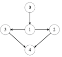
Figure 2: Communication graph.

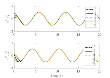
Figure 3: Performance of the distributed observer.

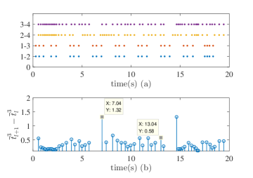
Figure 4: Event-triggered time instants.

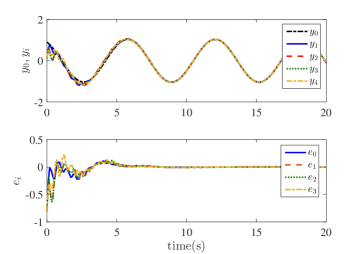
Figure 5: Control performance.

Table I: Event-triggered times for PETM-B under different $\iota_{e}$.

	$\iota_{e}=0.05$	$\iota_{e}=0.1$	$\iota_{e}=0.2$
sampled data	800	800	800
PET	390	324	271

VI Conclusions

In this paper, the PET cooperative output regulation problem is considered for strict feedback nonlinear multi-agent systems. We propose a new PET distributed observer and a PET output feedback control law for this problem. The communication between various agents can be asynchronous. Future works include considering PET output regulation for non-strict feedback nonlinear systems. For non-strict feedback nonlinear systems, the control effort and the states may be coupled with each other. This will make the problem more challenging.

VII Appendix

-A Two lemmas

In this section, we will present two key lemmas which will be used the in the proof of Theorems 1-2.

Lemma 3.

Consider the following system

$$\dot{x}= -\mu\Lambda_{1}\boldsymbol{x}_{d}+\mu\Lambda_{2}\boldsymbol{x}_{d}+\Lambda_{3}x+\mu\Lambda_{4}+\Lambda_{5}$$ (37)

where $x=(x_{1},x_{2},...,x_{N})^{\mathrm{T}}\in\mathbb{R}^{N}$, $\boldsymbol{x}_{d}=(x_{1}(t-d_{1}(t)),x_{2}(t-d_{2}(t)),...,x_{N}(t-d_{N}(t)))^{\mathrm{T}}\in\mathbb{R}^{N}$. $d_{i}(t)(i=1,2,...,N)\in\mathbb{R}$ are time-varying delays such that $0<d_{i}(t)\leq T$ with a positive constant $T$. $\mu>0$ is a positive constant. If $-\Lambda_{1}$ is a Hurwitz matrix and $\Lambda_{j}(j=2,3,4,5)\in\mathsf{E}(\gamma)$ with a positive constant $\gamma$, then there exist a sufficiently large $\mu$ and small $T$ such that $x\in\mathsf{E}(\gamma)$.

Proof:

(37) can be written as:

$$\dot{x}= -\mu\Lambda_{1}x+\mu\Lambda_{2}x+\mu\Lambda_{1}\eta-\mu\Lambda_{2}\eta$$

$$+\Lambda_{3}x+\mu\Lambda_{4}+\Lambda_{5}$$ (38)

where $\eta(t)=\mathrm{col}(\eta_{1}(t),\eta_{2}(t),...,\eta_{N}(t))$ with $\eta_{i}(t)=\int_{t-d_{i}(t)}^{t}\dot{x}_{i}(s)ds$.

Consider the following Lyapunov-Krasovskii function

$$V=\frac{1}{2}x^{\mathrm{T}}Px+\int_{t-T}^{t}(s-t+T)||\dot{x}(s)||^{2}ds$$ (39)

where $P$ is a positive definite matrix such that $P\Lambda_{1}+\Lambda_{1}^{\mathrm{T}}P=2I$.

Using (38), the derivative of $V$ is computed as:

$$\dot{V}\leq x^{\mathrm{T}}P(-\mu\Lambda_{1}x+\mu\Lambda_{2}x+\mu\Lambda_{1}\eta-\mu\Lambda_{2}\eta)$$

$$+x^{\mathrm{T}}P(\Lambda_{3}x+\mu\Lambda_{4}+\Lambda_{5})$$

$$+T||\dot{x}(t)||^{2}-\int_{t-T}^{t}||\dot{x}(s)||^{2}ds$$

$$= -\mu||x||^{2}+x^{\mathrm{T}}(\mu P\Lambda_{2}+P\Lambda_{3})x$$

$$+x^{\mathrm{T}}P(\mu\Lambda_{1}\eta-\mu\Lambda_{2}\eta)+x^{\mathrm{T}}P(\mu\Lambda_{4}+\Lambda_{5})$$

$$+T||\dot{x}(t)||^{2}-\int_{t-T}^{t}||\dot{x}(s)||^{2}ds.$$

Noting that $\Lambda_{j}(j=2,3,4,5)\in\mathsf{E}(\gamma)$ and using Young’s inequality, we have

$$\dot{V}\leq -\mu||x||^{2}+\overline{\mu}c_{1}\mathrm{e}^{-\gamma t}||x||^{2}$$

$$+\frac{\mu}{4}||x||^{2}+c_{2}\mu||\eta||^{2}$$

$$+\frac{\mu}{4}||x||^{2}+\overline{\mu}c_{3}\mathrm{e}^{-2\gamma t}$$

$$+T||\dot{x}(t)||^{2}-\int_{t-T}^{t}||\dot{x}(s)||^{2}ds$$ (40)

where $\overline{\mu}=\sqrt{\mu^{2}+1}$ and $c_{1},c_{2},c_{3}$ are some positive constants.

Meanwhile, using (38) for $||\dot{x}(t)||^{2}$ and Young’s inequality,

$$||\dot{x}(t)||^{2}\leq c_{4}\overline{\mu}^{2}||x||^{2}+c_{5}\mu^{2}||\eta||^{2}+c_{6}\overline{\mu}^{2}\mathrm{e}^{-2\gamma t}$$ (41)

where $c_{4},c_{5},c_{6}$ are some positive constants.

For $\eta$, by Jensen’s inequality [34], we have

$$\eta_{i}^{2}(t)=\left(\int_{t-d_{i}(t)}^{t}\dot{x}_{i}(s)ds\right)^{2}\leq T\int_{t-T}^{t}||\dot{x}_{i}(s)||^{2}ds,$$

then

$$||\eta||^{2}\leq T\int_{t-T}^{t}||\dot{x}(s)||^{2}ds.$$ (42)

Substituting (41) and (42) into (40), we get

$$\dot{V}\leq -\left(\frac{\mu}{2}-\overline{\mu}c_{1}\mathrm{e}^{-\gamma t}-Tc_{4}\overline{\mu}^{2}\right)||x||^{2}$$

$$-(1-Tc_{2}\mu-Tc_{5}\mu^{2})\int_{t-T}^{t}||\dot{x}(s)||^{2}ds$$

$$+\overline{\mu}c_{3}\mathrm{e}^{-2\gamma t}+Tc_{6}\overline{\mu}^{2}\mathrm{e}^{-2\gamma t}.$$

Then, for a positive constant $\gamma$, we have

$$\dot{V}+\gamma V\leq -\left(\frac{\mu}{2}-\overline{\mu}c_{1}\mathrm{e}^{-\gamma t}-Tc_{4}\overline{\mu}^{2}-\gamma||P||\right)||x||^{2}$$

$$-(1-Tc_{2}\mu-Tc_{5}\mu^{2}-\gamma T)\int_{t-T}^{t}||\dot{x}(s)||^{2}ds$$

$$+\overline{\mu}c_{3}\mathrm{e}^{-2\gamma t}+Tc_{6}\overline{\mu}^{2}\mathrm{e}^{-2\gamma t}.$$ (43)

Next, we will show $V$ does not exhibit finite time escape. From (43), we have

$$\dot{V}\leq \alpha V+\beta$$

where $\alpha,\beta$ are positive constants.

This means

$$V\leq V(0)\mathrm{e}^{\alpha t}-\frac{\beta}{\alpha}(1- \mathrm{e}^{\alpha t}).$$

Therefore, $V$ is bounded on finite time interval.

Moreover, on a finite time interval $[0,t_{0})\subset[0,+\infty)$, we have

$$V\leq V(0)\mathrm{e}^{(\alpha+\gamma)t}\mathrm{e}^{-\gamma t}-\frac{\beta}{\alpha}(1-\mathrm{e}^{\alpha t})\mathrm{e}^{\gamma t}\mathrm{e}^{-\gamma t}$$

$$\leq \max\{V(0)\mathrm{e}^{(\alpha+\gamma)t_{0}},\frac{\beta}{\alpha}(1-\mathrm{e}^{\alpha t_{0}})\mathrm{e}^{\gamma t_{0}}\}\mathrm{e}^{-\gamma t}$$

$$\leq c_{7}\mathrm{e}^{-\gamma t}$$ (44)

where $c_{7}$ is a positive constant.

On the other hand, for (43), there exists a finite time instant $t_{0}$, $\mu$ and $T$ such that

$$\frac{\mu}{2}-\overline{\mu}c_{1}\mathrm{e}^{-\gamma t_{0}}-Tc_{4}\overline{\mu}^{2}-\gamma||P||>0,$$

$$1-Tc_{2}\mu-Tc_{5}\mu^{2}-\gamma T>0.$$

Therefore,

$$\dot{V}\leq -\gamma V+c_{8}\mathrm{e}^{-2\gamma t}$$ (45)

for $\forall t\in[t_{0},+\infty)$ where $c_{8}$ is a positive constant.

Then, by solving the above inequality,

$$V\leq V(t_{0})\mathrm{e}^{-\gamma(t-t_{0})}-\frac{c_{8}}{\gamma}\mathrm{e}^{-2\gamma(t-t_{0})}+\frac{c_{8}}{\gamma}\mathrm{e}^{-\gamma t_{0}}\mathrm{e}^{-\gamma t}$$

$$\leq \max\{V(t_{0}),\frac{c_{8}}{\gamma}\}\mathrm{e}^{-\gamma t}\leq c_{9}\mathrm{e}^{-\gamma t}$$ (46)

for $\forall t\in[t_{0},+\infty)$ where $c_{9}$ is a positive constant.

Then by combining (44) and (46), we can complete the proof. ∎

Lemma 4.

Consider the system (37) in a special form by letting $\Lambda_{2}=\Lambda_{3}=\Lambda_{5}=0$. That is

$$\dot{x}= -\mu\Lambda_{1}\boldsymbol{x}_{d}+\mu\Lambda_{4}$$ (47)

where $-\Lambda_{1}$ is a Hurwitz matrix, $\Lambda_{4}\in\mathsf{E}(\gamma)$ with a positive constant $\gamma$. If $\mu,T$ satisfy

$$T<\mathrm{min} \left\{\frac{1}{6\mu||\Lambda_{1}||^{2}}-\frac{\gamma||P||}{3\mu^{2}||\Lambda_{1}||^{2}}\right.,$$

$$\left.\frac{1}{\mu||P\Lambda_{1}||+3\mu^{2}||P\Lambda_{1}||+\gamma}\right\}$$ (48)

where $P$ is a positive definite matrix such that $P\Lambda_{1}+\Lambda_{1}^{\mathrm{T}}P=2I$, then $x\in\mathsf{E}(\gamma)$.

Proof:

The proof follows the line of the proof of 1). Under the assumption that $\Lambda_{2}=\Lambda_{3}=\Lambda_{5}=0$, (37) can be written as:

$$\dot{x}= -\mu\Lambda_{1}x+\mu\Lambda_{1}\eta+\mu\Lambda_{4}$$ (49)

where $\eta(t)=\mathrm{col}(\eta_{1}(t),\eta_{2}(t),...,\eta_{N}(t))$ with $\eta_{i}(t)=\int_{t-d_{i}(t)}^{t}\dot{x}_{i}(s)ds$.

Consider a Lyapunov-Krasovskii function in the form of (39). By (49), we have

$$\dot{V}\leq x^{\mathrm{T}}P(-\mu\Lambda_{1}x+\mu\Lambda_{1}\eta+\mu\Lambda_{4})$$

$$+T||\dot{x}(t)||^{2}-\int_{t-T}^{t}||\dot{x}(s)||^{2}ds.$$

By Young’s inequality, we get

$$\dot{V}\leq -\mu||x||^{2}$$

$$+\frac{\mu}{4}||x||^{2}+\mu||P\Lambda_{1}||\cdot||\eta||^{2}$$

$$+\frac{\mu}{4}||x||^{2}+\mu c_{10}\mathrm{e}^{-2\gamma t}$$

$$+T||\dot{x}(t)||^{2}-\int_{t-T}^{t}||\dot{x}(s)||^{2}ds$$ (50)

where $c_{10}$ is a positive constant.

Meanwhile, using (49) for $||\dot{x}(t)||^{2}$ and by Young’s inequality

$$||\dot{x}(t)||^{2}\leq 3\mu^{2}||\Lambda_{1}||^{2}||x||^{2}+3\mu^{2}||\Lambda_{1}||^{2}||\eta||^{2}+c_{11}\mu^{2}\mathrm{e}^{-2\gamma t}$$ (51)

where $c_{11}$ is a positive constant.

Substituting (51) into (50),

$$\dot{V}\leq -\left(\frac{\mu}{2}-3T\mu^{2}||\Lambda_{1}||^{2}\right)||x||^{2}$$

$$-(1-T\mu||P\Lambda_{1}||-3T\mu^{2}||\Lambda_{1}||^{2})\int_{t-T}^{t}||\dot{x}(s)||^{2}ds$$

$$+\mu c_{10}\mathrm{e}^{-2\gamma t}+Tc_{11}\mu^{2}\mathrm{e}^{-2\gamma t}.$$

Then, for a positive constant $\gamma$, we have

$$\dot{V}+\gamma V$$

$$\leq -\left(\frac{\mu}{2}-3T\mu^{2}||\Lambda_{1}||^{2}-\gamma||P||\right)||x||^{2}$$

$$-(1-T\mu||P\Lambda_{1}||-3T\mu^{2}||\Lambda_{1}||^{2}-\gamma T)\int_{t-T}^{t}||\dot{x}(s)||^{2}ds$$

$$+\mu c_{10}\mathrm{e}^{-2\gamma t}+Tc_{11}\mu^{2}\mathrm{e}^{-2\gamma t}.$$ (52)

If the following inequality holds

$$\frac{\mu}{2}-3T\mu^{2}||\Lambda_{1}||^{2}-\gamma||P||>0,$$ (53)

$$1-T\mu||P\Lambda_{1}||-3T\mu^{2}||\Lambda_{1}||^{2}-\gamma T>0,$$ (54)

then we have

$$\dot{V}\leq -\gamma V+\mu c_{10}\mathrm{e}^{-2\gamma t}+Tc_{11}\mu^{2}\mathrm{e}^{-2\gamma t}.$$

By solving the above inequality, we can show $x\in\mathsf{E}(\gamma)$. Finally, note that (53)-(54) are equivalent to (48). This completes the proof. ∎

-B Proof of Theorems 1 and 2

Proof:

We will first prove Theorem 2. The proof is divided into the following two steps.

Step 1. Show $\tilde{A}_{i}\triangleq\hat{A}_{i}-A(i=1,2,...,N)$ converges to zero exponentially.

Note that (13) can be transformed into

$$\dot{\tilde{A}} =-\mu_{1}(\mathcal{H}\varotimes I)(\hat{\boldsymbol{A}}(\overline{t}_{l})-\overline{A})$$

$$=-\mu_{1}(\mathcal{H}\varotimes I)(\hat{\boldsymbol{A}}(\overline{t}_{l})-\hat{\boldsymbol{A}}(t_{k})+\tilde{\boldsymbol{A}}(t_{k}))$$ (55)

where $\overline{A}=\mathrm{col}(A,A,...,A)$, $\hat{A}=\mathrm{col}(\hat{A}_{1},\hat{A}_{2},...,\hat{A}_{N})$, $\tilde{A}=\hat{A}-\overline{A}$. $\hat{\boldsymbol{A}}(\overline{t}_{l})=\mathrm{col}(\hat{A}_{1}(\overline{t}_{l^{\prime}}^{1}),\hat{A}_{2}(\overline{t}_{l^{\prime}}^{2}),...,\hat{A}_{N}(\overline{t}_{l^{\prime}}^{N}))$, $\hat{\boldsymbol{A}}(t_{k})=\mathrm{col}(\hat{A}_{1}(t_{k^{\prime}}^{1}),\hat{A}_{2}(t_{k^{\prime}}^{2}),...,\hat{A}_{N}(t_{k^{\prime}}^{N}))$, $\tilde{\boldsymbol{A}}(t_{k})=\hat{\boldsymbol{A}}(t_{k})-\overline{A}$.

Let $\overline{\alpha}=\mathrm{vec}(\overline{A})$, $\hat{\alpha}=\mathrm{vec}(\hat{A})$, $\tilde{\alpha}=\mathrm{vec}(\tilde{A})$, $\hat{\boldsymbol{\alpha}}(\overline{t}_{l})=\mathrm{vec}(\hat{\boldsymbol{A}}(\overline{t}_{l}))$, $\hat{\boldsymbol{\alpha}}(t_{k})=\mathrm{vec}(\hat{\boldsymbol{A}}(t_{k}))$ and $\tilde{\boldsymbol{\alpha}}(t_{k})=\mathrm{vec}(\tilde{\boldsymbol{A}}(t_{k}))$, (55) becomes

$$\dot{\tilde{\alpha}} =-\mu_{1}(I\varotimes\mathcal{H}\varotimes I)(\hat{\boldsymbol{\alpha}}(\overline{t}_{l}^{i})-\hat{\boldsymbol{\alpha}}(t_{k})+\tilde{\boldsymbol{\alpha}}(t_{k})).$$

It follows that

$$\dot{\tilde{\alpha}} =-\mu_{1}(I\varotimes\mathcal{H}\varotimes I)\tilde{\boldsymbol{\alpha}}(t_{k})+\mu_{1}\Lambda_{A}$$ (56)

where $\Lambda_{A}=(I\varotimes\mathcal{H}\varotimes I)(\hat{\boldsymbol{\alpha}}(\overline{t}_{l})-\hat{\boldsymbol{\alpha}}(t_{k}))$.

From the event-triggered condition (16), we know $\Lambda_{A}\in\mathsf{E}(\gamma_{A})$. Then, let $d_{i}(t)=t-t_{k}^{i}$ in (56) and use Lemma 3 in Appendix A, we can show $\tilde{\alpha}\in\mathsf{E}(\gamma_{A})$, $i.e.$, $\tilde{A}_{i}\in\mathsf{E}(\gamma_{A})(i=1,2,...,N)$.

Step 2. Show $\tilde{\nu}_{i}\triangleq\hat{\nu}_{i}-\nu(i=1,2,...,N)$ converges to zero exponentially.

Let

$$z_{i}(t) =\mathrm{e}^{-At}\hat{\nu}_{i}(t)(i=0,1,...,n)$$ (57)

where $z_{0}(t)=\mathrm{e}^{-At}\hat{\nu}_{0}(t)=\mathrm{e}^{-At}\nu(t)=\nu(0).$

Then, (14) can be expressed as:

$$\dot{z}_{i}= -\mathrm{e}^{-At}A\hat{\nu}_{i}(t)+\mathrm{e}^{-At}\hat{A}_{i}\hat{\nu}_{i}(t)$$

$$+\mathrm{e}^{-At}\mu_{2}\sum_{j=0}^{N}a_{ij}(\overline{\nu}_{j}(t,\overline{t}_{l^{\prime}}^{j})-\overline{\nu}_{i}(t,\overline{t}_{l}^{i})).$$

The above inequality can be written as:

$$\dot{z}_{i}= \Delta_{i}^{1}+\mu_{2}\sum_{j=0}^{N}a_{ij}\left(\Delta_{j}^{2}-\Delta_{i}^{2}\right)$$

$$+\mu_{2}\sum_{j=0}^{N}a_{ij}\left(\Delta_{j}^{3}-\Delta_{i}^{3}\right)$$

$$+\mu_{2}\sum_{j=0}^{N}a_{ij}(z_{j}(t_{k^{\prime}}^{j})-z_{i}(t_{k}^{i}))$$

where

$$\Delta_{i}^{1}=\mathrm{e}^{-At}\hat{A}_{i}\hat{\nu}_{i}(t)-\mathrm{e}^{-At}A\hat{\nu}_{i}(t),$$ (58)

$$\Delta_{i}^{2}=\mathrm{e}^{-At}\left(\mathrm{e}^{\hat{A}_{i}(\overline{t}_{l}^{i})(t-\overline{t}_{l}^{i})}\hat{\nu}_{i}(\overline{t}_{l}^{i})-\mathrm{e}^{\hat{A}_{i}(\overline{t}_{l}^{i})(t-t_{k}^{i})}\hat{\nu}_{i}(t_{k}^{i})\right),$$ (59)

$$\Delta_{i}^{3}=\mathrm{e}^{-At}\left(\mathrm{e}^{\hat{A}_{i}(\overline{t}_{l}^{i})(t-t_{k}^{i})}\hat{\nu}_{i}(t_{k}^{i})-\mathrm{e}^{A(t-t_{k}^{i})}\hat{\nu}_{i}(t_{k}^{i})\right).$$ (60)

By considering agent $i=1,2,...,N$, we have

$$\dot{\tilde{z}}= -\mu_{2}(\mathcal{H}\varotimes I)\tilde{\boldsymbol{z}}(t_{k})$$

$$+\Delta^{1}-\mu_{2}(\mathcal{H}\varotimes I)\Delta^{2}-\mu_{2}(\mathcal{H}\varotimes I)\Delta^{3}$$ (61)

where $\tilde{\boldsymbol{z}}(t_{k})=\mathrm{col}(z_{1}(t_{k^{\prime}}^{1}),z_{2}(t_{k^{\prime}}^{2}),...,z_{N}(t_{k^{\prime}}^{N}))$, $\Delta^{1}=\mathrm{col}(\Delta_{1}^{1},\Delta_{2}^{1},...,\Delta_{N}^{1})$, $\Delta^{2}=\mathrm{col}(\Delta_{1}^{2},\Delta_{2}^{2},...,\Delta_{N}^{2})$, $\Delta^{3}=\mathrm{col}(\Delta_{1}^{3},\Delta_{2}^{3},...,\Delta_{N}^{3})$.

In the following, we will have an analysis on $\Delta^{1},\Delta^{2}$ and $\Delta^{3}$.

For $\Delta_{i}^{1}$ in $\Delta^{1}$, we have

$$\Delta_{i}^{1} =\mathrm{e}^{-At}\hat{A}_{i}\hat{\nu}_{i}(t)-\mathrm{e}^{-At}A\hat{\nu}_{i}(t)$$

$$=\mathrm{e}^{-At}\tilde{A}_{i}\mathrm{e}^{At}\tilde{z}_{i}+\mathrm{e}^{-At}\tilde{A}_{i}\mathrm{e}^{At}z_{0}.$$

This implies that

$$\Delta^{1} =\Lambda_{1}\tilde{z}+\Lambda_{1}\bar{z}$$ (62)

where $\Lambda_{1}=\mathrm{diag}(\mathrm{e}^{-At}\tilde{A}_{1}\mathrm{e}^{At},\mathrm{e}^{-At}\tilde{A}_{2}\mathrm{e}^{At},...,\mathrm{e}^{-At}\tilde{A}_{N}\mathrm{e}^{At})$, $\bar{z}=\mathrm{col}(z_{0},z_{0},...,z_{0})$.

For $i=1,2,...,N$, using the result in Step 1 and Lemma 1-1), we get

$$||\mathrm{e}^{-At}\tilde{A}_{i}\mathrm{e}^{At}||\leq||\mathrm{e}^{-At}||\cdot||\tilde{A}_{i}||\cdot||\mathrm{e}^{-At}||=||\tilde{A}_{i}||\in\mathsf{E}(\gamma_{A}).$$

This implies that $||\Lambda_{1}||\in\mathsf{E}(\gamma_{A})$ and $||\Lambda_{1}\bar{z}||\in\mathsf{E}(\gamma_{A})$.

For $\Delta_{i}^{2}$ in $\Delta^{2}$, according to (59), we have

$$\Delta_{i}^{2} =\mathrm{e}^{-At}\mathrm{e}^{\hat{A}_{i}(\overline{t}_{l}^{i})(t-t_{k}^{i})}\left(\mathrm{e}^{\hat{A}_{i}(\overline{t}_{l}^{i})(t_{k}^{i}-\overline{t}_{l}^{i})}\hat{\nu}_{i}(\overline{t}_{l}^{i})-\hat{\nu}_{i}(t_{k}^{i})\right).$$

Note that $||\mathrm{e}^{-At}\mathrm{e}^{\hat{A}_{i}(\overline{t}_{l}^{i})(t-t_{k}^{i})}||$ are bounded by Lemma 1-1). According to (16), we get $||\Delta_{i}^{2}||\in\mathsf{E}(\gamma_{\nu}).$ Thus, $||(\mathcal{H}\varotimes I)\Delta^{2}||\in\mathsf{E}(\gamma_{\nu}).$

For $\Delta_{i}^{3}$ in $\Delta^{3}$, according to (60), we have

$$\Delta_{i}^{3} =\mathrm{e}^{-At}\left(\mathrm{e}^{\hat{A}_{i}(t-t_{k}^{i})}-\mathrm{e}^{A(t-t_{k}^{i})}\right)\mathrm{e}^{At_{k}^{i}}z_{i}(t_{k}^{i}).$$

This indicates that

$$\Delta^{3}=\Lambda_{2}\tilde{\boldsymbol{z}}(t_{k})+\Lambda_{2}\bar{z}$$ (63)

where $\bar{z}=\mathrm{col}(z_{0},z_{0},...,z_{0})$, $\Lambda_{2}=\mathrm{diag}(\mathrm{e}^{-At}(\mathrm{e}^{\hat{A}_{1}(t-t_{k^{\prime}}^{1})}-\mathrm{e}^{A(t-t_{k^{\prime}}^{1})})\mathrm{e}^{At_{k^{\prime}}^{1}},...,\mathrm{e}^{-At}(\mathrm{e}^{\hat{A}_{N}(t-t_{k^{\prime}}^{N})}-\mathrm{e}^{A(t-t_{k^{\prime}}^{N})})\mathrm{e}^{At_{k^{\prime}}^{N}})$.

Note that for any entry in $\Lambda_{2}$, using Lemma 1-2), we have

$$||\mathrm{e}^{-At}(\mathrm{e}^{\hat{A}_{i}(t-t_{k}^{i})}-\mathrm{e}^{A(t-t_{k}^{i})})\mathrm{e}^{At_{k}^{i}}||$$

$$\leq ||\mathrm{e}^{-At}||\cdot||\mathrm{e}^{\hat{A}_{i}(t-t_{k}^{i})}-\mathrm{e}^{A(t-t_{k}^{i})}||\cdot||\mathrm{e}^{At_{k}^{i}}||$$

$$\leq ||\hat{A}_{i}-A||\mathrm{e}^{||(\hat{A}_{i}-A)(t-t_{k}^{i})||+||A(t-t_{k}^{i})||}\in\mathsf{E}(\gamma_{A}).$$

This implies that $||\Lambda_{2}||\in\mathsf{E}(\gamma_{A})$ and $||\Lambda_{2}\bar{z}||\in\mathsf{E}(\gamma_{A})$.

Based on (62) and (63), (61) becomes

$$\dot{\tilde{z}}= -\mu_{2}(\mathcal{H}\varotimes I)\tilde{\boldsymbol{z}}(t_{k})$$

$$+\Lambda_{1}\tilde{z}+\Lambda_{1}\bar{z}-\mu_{2}(\mathcal{H}\varotimes I)\Delta^{2}$$

$$-\mu_{2}(\mathcal{H}\varotimes I)(\Lambda_{2}\tilde{\boldsymbol{z}}(t_{k})+\Lambda_{2}\bar{z})$$

$$= -\mu_{2}(\mathcal{H}\varotimes I)\tilde{\boldsymbol{z}}(t_{k})-\mu_{2}(\mathcal{H}\varotimes I)\Lambda_{2}\tilde{\boldsymbol{z}}(t_{k})+\Lambda_{1}\tilde{z}$$

$$-\mu_{2}(\mathcal{H}\varotimes I)\Delta^{2}-\mu_{2}(\mathcal{H}\varotimes I)\Lambda_{2}\bar{z}+\Lambda_{1}\bar{z}.$$ (64)

Let $\mathcal{H}\varotimes I=\overline{\Lambda}_{1}$, $-\mu_{2}(\mathcal{H}\varotimes I)\Lambda_{2}=\overline{\Lambda}_{2}$, $\Lambda_{1}=\overline{\Lambda}_{3}$, $-(\mathcal{H}\varotimes I)\Delta^{2}-(\mathcal{H}\varotimes I)\Lambda_{2}\bar{z}=\overline{\Lambda}_{4}$, $\Lambda_{1}\bar{z}=\overline{\Lambda}_{5}$.

Then, (64) is expressed as

$$\dot{\tilde{z}}= -\mu_{2}\overline{\Lambda}_{1}\tilde{\boldsymbol{z}}(t_{k})+\mu_{2}\overline{\Lambda}_{2}\tilde{\boldsymbol{z}}(t_{k})+\overline{\Lambda}_{3}\tilde{z}$$

$$+\mu_{2}\overline{\Lambda}_{4}+\overline{\Lambda}_{5}$$

where $\overline{\Lambda}_{2},\overline{\Lambda}_{3},\overline{\Lambda}_{4},\overline{\Lambda}_{5}\in\mathsf{E}(\mathrm{min}(\gamma_{A},\gamma_{\nu})).$

Using Lemma 3 in Appendix A, we can show $\tilde{z}\in\mathsf{E}(\mathrm{min}(\gamma_{A},\gamma_{\nu}))$. Note that

$$||\tilde{\nu}_{i}||=||\mathrm{e}^{-At}\tilde{\nu}_{i}||\leq||\tilde{z}||\in\mathsf{E}(\mathrm{min}(\gamma_{A},\gamma_{\nu}))$$

for $i=1,2,...,N$. Therefore, Theorem 2 is proved.

Next, we will prove Theorem 1. The proof follows the line of Step 2 by using the real value of $A$ instead of $\hat{A}_{i}$. In this case, (61) becomes

$$\dot{\tilde{z}}= -\mu_{2}(\mathcal{H}\varotimes I)\tilde{\boldsymbol{z}}(t_{k})+\mu_{2}\overline{\Lambda}_{4}$$

where $\overline{\Lambda}_{4}\in\mathsf{E}(\gamma_{\nu}).$

Then, by Lemma 4, we can show $||\tilde{\nu}_{i}||=||\mathrm{e}^{-At}\tilde{\nu}_{i}||\leq||\tilde{z}||\in\mathsf{E}(\gamma_{\nu})$ if $T$ satisfies (12). This completes the proof. ∎

-C Proof of Proposition 1

Proof:

First, from (17), we know

$$\xi_{i2} =\overline{f}_{i1}(\overline{z}_{i},\tilde{\eta}_{i1},\overline{x}_{i1},\nu,w)+b_{i1}(w)\overline{x}_{i2}$$

$$\triangleq\overline{\xi}_{i2}(\overline{z}_{i},\tilde{\eta}_{i1},\overline{x}_{i1},\overline{x}_{i2},\nu,w).$$

This shows (18) holds with $j=2$. Meanwhile, we have

$$\overline{x}_{i2} =(\xi_{i2}-\overline{f}_{i1}(\overline{z}_{i},\tilde{\eta}_{i1},\xi_{i1},\nu,w))/b_{i1}(w)$$

$$\triangleq\chi_{i2}(\overline{z}_{i},\tilde{\eta}_{i1},\xi_{i1},\xi_{i2},\nu,w).$$

This shows (19) holds with $j=2$.

For $j=3$, by (17) and (8), we know

$$\xi_{i3}\triangleq\dot{\xi}_{i2}= \frac{\partial\overline{\xi}_{i2}}{\partial\overline{z}_{i}}\overline{f}_{i0}+\frac{\partial\overline{\xi}_{i2}}{\partial\tilde{\eta}_{i1}}(M_{ij}\tilde{\eta}_{ij}+g_{ij})$$

$$+\frac{\partial\overline{\xi}_{i2}}{\partial\overline{x}_{i1}}\left(\overline{f}_{i1}+b_{i1}(w)\overline{x}_{i2}\right)$$

$$+\frac{\partial\overline{\xi}_{i2}}{\partial\overline{x}_{i2}}\left(\overline{f}_{i2}+b_{i2}(w)\overline{x}_{i3}\right)+\frac{\partial\overline{\xi}_{i2}}{\partial\nu}A\nu$$

$$\triangleq \overline{\xi}_{i3}(\overline{z}_{i},\tilde{\eta}_{i1},\tilde{\eta}_{i2},\overline{x}_{i1},\overline{x}_{i2},\overline{x}_{i3},\nu,w).$$

This shows (18) holds with $j=3$. Similarly, we can show (19) holds with $j\geq 4$. This completes the proof. ∎

-D Proof of Proposition 2

Proof:

For $j=1$, we have

$$\dot{\alpha}_{i1}=-Q_{i1}\dot{\zeta}_{i1}=-Q_{i1}(\zeta_{i2}-Q_{i1}\zeta_{i1})\leq\vartheta_{i1}(Q_{i1})(|\zeta_{i1}|+|\zeta_{i2}|).$$

For $j=2$, using the above inequality, we have

$$\dot{\alpha}_{i2} =-Q_{i2}\dot{\zeta}_{i2}=-Q_{i2}(\zeta_{i3}+\alpha_{i2}-\dot{\alpha}_{i1})$$

$$=-Q_{i2}(\zeta_{i3}-Q_{i2}\zeta_{i2}-\dot{\alpha}_{i1})$$

$$\leq\vartheta_{i2}(Q_{i1},Q_{i2})(|\zeta_{i1}|+|\zeta_{i2}|+|\zeta_{i3}|).$$

By repeating the above procedures for $j=3,4,...,n$, we can complete the proof. ∎

-E Proof of Lemma 2

Proof:

The proof is divided into the following steps. We will analyze each term in the Lyapunov function (24).

Step 1). Analysis of $V_{i0}(\overline{z}_{i})$.

According to Lemma 11.1 in [3], we know when $X_{i}\in\Omega_{R}$, there exists a positive constant gain $\overline{\mu}_{i0}(R)$ related with $R$ such that

$$\left\|\frac{\partial V_{i0}}{\partial\overline{z}_{i}}\right\|\cdot||\overline{f}_{i0}(\overline{z}_{i},\zeta_{1i},\nu,w)-\overline{f}_{i0}(\overline{z}_{i},0,\nu,w)||$$

$$\leq \overline{\mu}_{i0}(R)||\overline{z}_{i}||\cdot|\zeta_{1i}|.$$

Then, using Assumption 4 and Young’s inequality, the derivative of $V_{i0}$ can be computed as:

$$\dot{V}_{i0}(\overline{z}_{i})= \frac{\partial V_{i0}}{\partial\overline{z}_{i}}\overline{f}_{i0}(\overline{z}_{i},\zeta_{1i},\nu,w)$$

$$= \frac{\partial V_{i0}}{\partial\overline{z}_{i}}\overline{f}_{i0}(\overline{z}_{i},0,\nu,w)$$

$$+\frac{\partial V_{i0}}{\partial\overline{z}_{i}}(\overline{f}_{i0}(\overline{z}_{i},\zeta_{1i},\nu,w)-\overline{f}_{i0}(\overline{z}_{i},0,\nu,w))$$

$$\leq -\gamma_{i0}||\overline{z}_{i}||^{2}+\overline{\mu}_{i0}(R)||\overline{z}_{i}||\cdot|\zeta_{1i}|$$

$$\leq -\frac{\gamma_{i0}|}{2}|\overline{z}_{i}||^{2}+\mu_{i0}(R)\zeta_{1i}^{2}$$

where $\mu_{i0}(R)$ is a positive constant related with $R$.

Then, let $V_{i}^{z}=\frac{V_{i0}(\overline{z}_{i})}{L_{i0}}$, we have

$$\dot{V}_{i}^{z}(\overline{z}_{i})\leq -\frac{\gamma_{i0}}{2L_{i0}}||\overline{z}_{i}||^{2}+\frac{\mu_{i0}(R)}{L_{i0}}\zeta_{1i}^{2}.$$

Step 2). Analysis of $\frac{\tilde{\eta}_{ij}^{\mathrm{T}}P_{ij}\tilde{\eta}_{ij}}{L_{ij}}$.

Consider the following Lyapunov function $V_{ij}^{\eta}=\frac{\tilde{\eta}_{ij}^{\mathrm{T}}P_{ij}\tilde{\eta}_{ij}}{L_{ij}}.$ Then using Lemma 11.1 in [3] and the transformed system (23), the derivative of $V_{ij}^{\eta}$ is

$$\dot{V}_{ij}^{\eta}= \frac{1}{L_{ij}}\tilde{\eta}_{ij}^{\mathrm{T}}(P_{ij}M_{ij}+M_{ij}^{\mathrm{T}}P_{ij})\tilde{\eta}_{ij}$$

$$+\frac{1}{L_{ij}}\tilde{\eta}_{ij}^{\mathrm{T}}P_{ij}\overline{h}_{ij}(\overline{z}_{i},\tilde{\eta}_{i1},...,\tilde{\eta}_{i,j-1},\zeta_{i1},...,\zeta_{ij},\nu,w)$$

$$\leq -\frac{\beta_{ij}}{2L_{ij}}||\tilde{\eta}_{ij}||^{2}+\frac{\overline{\gamma}_{ij}(\overline{z}_{i})}{L_{ij}}||\overline{z}_{i}||^{2}+\sum_{k=1}^{j-1}\frac{\overline{\varrho}_{ijk}(\tilde{\eta}_{ik})}{L_{ij}}||\tilde{\eta}_{ik}||^{2}$$

$$+\sum_{k=1}^{j}\frac{\overline{\mu}_{ijk}(\zeta_{ik})}{L_{ij}}\zeta_{ik}^{2}$$ (65)

where $\overline{\gamma}_{ij}(\overline{z}_{i}),\overline{\varrho}_{ijk}(\tilde{\eta}_{ik}),\overline{\mu}_{ijk}(\zeta_{ik})$ are continuous functions.

Note that by (25), for $\forall X_{i}\in\Omega_{R}$,

$$c_{P_{ij}}||\tilde{\eta}_{ij}||^{2}\leq\tilde{\eta}_{ij}^{T}P_{ij}\tilde{\eta}_{ij}\leq L_{ij}R^{2}$$

where $c_{P_{ij}}>0$ denotes the minimum eigenvalue of matrix $P_{ij}$.

Hence, (65) can be expressed as:

$$\dot{V}_{ij}^{\eta}\leq -\frac{\beta_{ij}}{2L_{ij}}||\tilde{\eta}_{ij}||^{2}+\frac{\gamma_{ij}(R)}{L_{ij}}||\overline{z}_{i}||^{2}+\sum_{k=1}^{j-1}\frac{\varrho_{ijk}(RL_{ik})}{L_{ij}}||\tilde{\eta}_{ik}||^{2}$$

$$+\frac{\mu_{ij}(R)}{L_{ij}}\sum_{k=1}^{j}\zeta_{ik}^{2}$$

where $\gamma_{ij}(R),\varrho_{ij}(RL_{ik}),\mu_{ij}(R)$ are positive gains related with $R$ and $L_{ik}$.

Step 3). Analysis of $V_{i}^{z}$ and $V_{ij}^{\eta}$.

Consider the following Lyapunov function

$$W_{i}\triangleq V_{i}^{z}+\sum_{j=1}^{n}V_{ij}^{\eta}.$$

We can obtain

$$\dot{W}_{i}= \dot{V}_{i}^{z}(\overline{z}_{i})+\sum_{j=1}^{n}\dot{V}_{ij}^{\eta}$$

$$\leq -\left(\frac{\gamma_{i0}}{2L_{i0}}-\sum_{j=1}^{n}\frac{\gamma_{ij}(R)}{L_{ij}}\right)||\overline{z}_{i}||^{2}$$

$$-\sum_{j=1}^{n}\left(\frac{\beta_{ij}}{2L_{ij}}-\sum_{k=j+1}^{n}\frac{\varrho_{ijk}(RL_{ik})}{L_{ik}}\right)||\tilde{\eta}_{ij}||^{2}$$

$$+\left(\sum_{j=0}^{n}\frac{\mu_{ij}(R)}{L_{ij}}\right)\zeta_{i1}^{2}+\sum_{k=2}^{n}\left(\sum_{j=k}^{n}\frac{\mu_{ij}(R)}{L_{ij}}\right)\zeta_{ik}^{2}.$$ (66)

Thus there exist sufficiently large scaling gains $L_{ij}$ and positive constants $\tilde{\gamma}_{i},\tilde{\varrho}_{i}$ such that

$$\frac{\gamma_{i0}}{2L_{i0}}-\sum_{j=1}^{n}\frac{\gamma_{ij}(R)}{L_{ij}} \geq\tilde{\gamma}_{i},$$

$$\frac{\beta_{ij}}{2L_{ij}}-\sum_{k=j+1}^{n}\frac{\varrho_{ijk}(RL_{ij})}{L_{ik}} \geq\tilde{\varrho}_{i},j=1,...,n,$$

$$\sum_{j=0}^{n}\frac{\mu_{ij}(R)}{L_{ij}} \leq\frac{1}{4}.$$

Hence, we have

$$\dot{W}_{i}\leq-\tilde{\gamma}_{i}||\overline{z}_{i}||^{2}-\tilde{\varrho}_{i}\sum_{k=1}^{j}||\tilde{\eta}_{ij}||^{2}+\frac{1}{4}\sum_{j=1}^{n}\zeta_{ij}^{2}.$$

Step 4). Analysis of $\frac{1}{2}\zeta_{ij}^{2}$.

Consider Lyapunov function $V_{ij}^{\zeta}=\frac{1}{2}\zeta_{ij}^{2}.$ By (23), (22) and Proposition 2, we have for $j=1,...,n-1$,

$$\dot{V}_{ij}^{\zeta}= \zeta_{ij}(\zeta_{i,j+1}-Q_{ij}\zeta_{ij}-\dot{\alpha}_{i,j-1})$$

$$\leq -Q_{ij}\zeta_{ij}^{2}+\zeta_{ij}\zeta_{i,j+1}$$

$$+|\zeta_{ij}|\vartheta_{ij}(Q_{i1},Q_{i2},...,Q_{i,j-1})(|\zeta_{i1}|+\cdots+|\zeta_{ij}|)$$

$$\leq -\left(Q_{ij}-\overline{\vartheta}_{ij}(Q_{i1},...,Q_{i,j-1})\right)\zeta_{ij}^{2}$$

$$+\frac{\zeta_{i,j+1}^{2}}{2}+\sum_{k=1}^{j-1}\zeta_{ik}^{2}$$

where $\overline{\vartheta}_{ij}(Q_{i1},...,Q_{i,j-1})$ is a positive constant depending on $Q_{i1},...,Q_{i,j-1}$.

Let

$$Q_{ij}=\overline{\vartheta}_{ij}(Q_{i1},...,Q_{i,j-1})+n.$$

We obtain

$$\dot{V}_{ij}^{\zeta}\leq -n\zeta_{ij}^{2}+\frac{\zeta_{i,j+1}^{2}}{2}+\sum_{k=1}^{j-1}\zeta_{ik}^{2}(j=1,...,n-1).$$

Then let $V_{i}^{\zeta}=\sum_{j=1}^{n}\frac{\zeta_{ij}^{2}}{2}$ and use (23). We have

$$\dot{V}_{i}^{\zeta}\leq -\sum_{j=1}^{n-1}\zeta_{ij}^{2}+\zeta_{in}(\overline{\phi}_{i}-\dot{\alpha}_{i,n-1}+b_{in}(w)\overline{u}_{i}).$$

Using Proposition 2 and Young’s inequality, for $\forall X_{i}\in\Omega_{R}$, we obtain

$$\dot{V}_{i}^{\zeta}\leq -\frac{1}{2}\sum_{j=1}^{n-1}\zeta_{ij}^{2}+\zeta_{in}b_{in}(w)\overline{u}_{i}$$

$$+\frac{\tilde{\gamma}_{i}}{2}||\overline{z}_{i}||^{2}+\frac{\tilde{\varrho}_{i}}{2}\sum_{j=1}^{n-1}||\tilde{\eta}_{ij}||^{2}+\mu_{i}^{*}(R)\zeta_{in}^{2}$$ (67)

where $\mu_{i}^{*}(R)$ is a positive constant related with $R$.

5) Analysis of $V_{i}$.

Finally, based on (66) and (67), the derivative of $V_{i}$ can be computed as

$$\dot{V}_{i}\leq -\frac{\tilde{\gamma}_{i}}{2}||\overline{z}_{i}||^{2}-\frac{\tilde{\varrho}_{i}}{2}\sum_{k=1}^{j}||\tilde{\eta}_{ij}||^{2}-\frac{1}{4}\sum_{j=1}^{n-1}\zeta_{ij}^{2}$$

$$-(b_{in}(w)K_{i}(R)-\mu_{i}^{*}(R))\zeta_{in}^{2}$$

$$+\zeta_{in}b_{in}(w)(\overline{u}_{i}-\overline{u}_{i}^{*})$$

where $\overline{u}_{i}^{*}$ is given by (26).

Hence, if

$$K_{i}(R)>\mu_{i}^{*}(R)/b_{in}(w)$$

we obtain (27). The proof is completed. ∎

-F Proof of Theorems 3 and 4

Proof:

We only provide the proof for Theorem 4. The proof of Theorem 3 follows. The proof is divided into the following steps.

Step 1). Construction of the estimation error system.

Using the transformed system (20) and the observer (28), define the estimation error as $\tilde{\xi}_{ij}=\xi_{ij}-\hat{\xi}_{ij}(i=1,2,...,N;j=1,2,...,n)$. Then, the estimation error system is constructed as:

$$\dot{\tilde{\xi}}_{i1}= \tilde{\xi}_{i2}-\Gamma_{i}d_{1}\tilde{\xi}_{i1}+\Gamma_{i}d_{1}(\hat{e}_{i}(\overline{\tau}_{q}^{i})-e_{i}),$$

$$\dot{\tilde{\xi}}_{i2}= \tilde{\xi}_{i3}-\Gamma_{i}^{2}d_{2}\tilde{\xi}_{i1}+\Gamma_{i}^{2}d_{2}(\hat{e}_{i}(\overline{\tau}_{q}^{i})-e_{i}),$$

$$\vdots$$

$$\dot{\tilde{\xi}}_{in}= -\Gamma_{i}^{n}d_{n}\tilde{\xi}_{i1}+\Gamma_{i}^{n}d_{n}(\hat{e}_{i}(\overline{\tau}_{q}^{i})-e_{i})$$

$$+\phi_{i}+(b_{in}(w)-\hat{b}_{in})\overline{u}_{i}.$$

Let $\epsilon_{ij}=\Gamma_{i}^{n-j}\tilde{\xi}_{ij}(j=1,2,...,n)$. It follows that

$$\dot{\epsilon}_{i}=\Gamma_{i}D_{\epsilon}\epsilon_{i}+H_{i}$$ (68)

where $\epsilon_{i}=\mathrm{col}(\epsilon_{i1},\epsilon_{i2},...,\epsilon_{in})$,

$$D_{\epsilon}=\left[\begin{array}[]{cccc}-d_{1}&1\\ \vdots&&\ddots\\ -d_{n-1}&&&1\\ -d_{n}\end{array}\right],$$

$$H_{i}=H_{i1}+H_{i2}$$

with

$$H_{i1}=\Gamma_{i}^{n}(\hat{e}_{i}(\overline{\tau}_{q}^{i})-e_{i}(t))\mathrm{col}(d_{1},...,d_{n}),$$

$$H_{i2}=\mathrm{col}(0,0,...,\overline{\phi}_{i}+(b_{in}(w)-\hat{b}_{in})\overline{u}_{i}).$$

Step 2). Construction of the Lyapunov functions.

Note that since the design parameters $d_{1},...,d_{n}$ are the coefficients of some Hurwitz polynomial $s^{n}+d_{1}s^{n-1}+\cdots+d_{n-1}s+d_{n}$, $D_{\epsilon}$ is Hurwtiz. This indicates that we can find a positive definite matrix $P$ such that $PD_{\epsilon}+D_{\epsilon}^{\mathrm{T}}P\leq-I$. Then, take the following Lyapunov function $V_{i}^{\epsilon}=\epsilon_{i}^{\mathrm{T}}P\epsilon_{i}$. The derivative of $V_{i}^{\epsilon}$ is given by

$$\dot{V}_{i}^{\epsilon}= -\Gamma_{i}||\epsilon_{i}||^{2}+2\epsilon_{i}^{\mathrm{T}}PH_{i1}+2\epsilon_{i}^{\mathrm{T}}PH_{i2}.$$ (69)

For $\epsilon_{i}^{\mathrm{T}}PH_{i1}$, by Young’s inequality and (29), we have

$$\epsilon_{i}^{\mathrm{T}}PH_{i1} \leq\frac{\Gamma_{i}}{5}||\epsilon_{i}||^{2}+\sigma_{i1}(\Gamma_{i})(\hat{e}_{i}(\overline{\tau}_{q}^{i})-e_{i}(t))^{2}$$ (70)

where $\sigma_{i1}(\Gamma_{i})$ is a positive constant related with $\Gamma_{i}.$

For $\epsilon_{i}^{T}PH_{i2}$, note that $\phi_{i}(0,...,0,\nu,w)=0$. Then when $X_{i}\in\Omega_{R}$ we have

$$\epsilon_{i}^{T}PH_{i2}\leq \frac{\Gamma_{i}}{5}||\epsilon_{i}||^{2}+\sigma_{i2}(R)(\overline{z}_{i}^{2}+\sum_{j=1}^{n}(\tilde{\eta}_{ij}^{2}+\zeta_{ij}^{2}))$$

$$+\sigma_{i2}(R)(\overline{u}_{i}-\overline{u}_{i}^{*})^{2}$$ (71)

where $\sigma_{i2}(R_{i})$ is a positive constant related with $R_{i}.$

Finally, consider the following Lyapunov function in logarithm form

$$\mathcal{V}_{i}=V_{i}+\frac{\ln(1+V_{i}^{\epsilon})}{\ln(1+\varsigma_{i}(\Gamma_{i}))}.$$ (72)

Assume $V_{i}^{\epsilon}(0)\leq R_{\epsilon}$ for $\forall X_{i}\in B_{r}$ with a positive constant $R_{\epsilon}$. Then $\varsigma_{i}(\Gamma_{i})$ is selected to be a polynomial function with respect to $\Gamma_{i}$ such that $\frac{\ln(1+R_{\epsilon})}{\ln(1+\varsigma_{i}(\Gamma_{i}))}\leq\frac{\Delta_{R}}{2}$.

Based on Lemma 2 and (69)-(71), the derivative of $\mathcal{V}_{i}$ is computed as:

$$\mathcal{\dot{V}}_{i}\leq -\tilde{\gamma}_{i}||\overline{z}_{i}||^{2}-\tilde{\varrho}_{i}\sum_{j=1}^{n}||\tilde{\eta}_{ij}||^{2}-\sum_{j=1}^{n}\zeta_{ij}^{2}$$

$$+\Upsilon_{i1}+\Upsilon_{i2}+\Upsilon_{i3}+\Upsilon_{i4}$$ (73)

where

$$\Upsilon_{i1}= -\frac{\Gamma_{i}}{5\ln(1+\varsigma_{i}(\Gamma_{i}))}\frac{||\mathit{\epsilon_{i}}||^{2}}{1+||P||||\mathit{\epsilon_{i}}||^{2}}$$

$$+\frac{2\sigma_{i2}(R)(\widetilde{u}_{i}-\overline{u}_{i}^{*})^{2}}{\ln(1+\varsigma_{i}(\Gamma_{i}))},$$

$$\Upsilon_{i2}= \frac{2\sigma_{i2}(R)\left(\overline{z}_{i}^{2}+\sum_{j=1}^{2}(\tilde{\eta}_{ij}^{2}+\zeta_{ij}^{2})\right)}{\ln(1+\varsigma_{i}(\Gamma_{i}))},$$

$$\Upsilon_{i3} =\frac{2\sigma_{i2}(R)(\overline{u}_{i}-\widetilde{u}_{i})^{2}}{\ln(1+\varsigma_{i}(\Gamma_{i}))},$$

$$\Upsilon_{i4}= \frac{2\sigma_{i1}(\Gamma_{i})(\hat{e}_{i}(\overline{\tau}_{q}^{i})-e_{i}(t))^{2}}{\ln(1+\varsigma_{i}(\Gamma_{i}))},$$

$$\widetilde{u}_{i} =\omega_{i}(t)-\Psi_{in}\eta_{in}(t)=\mathrm{sat}_{\mathcal{R}}(K_{i}(R)\hat{\zeta}_{in}(t)),$$

$$\overline{u}_{i}=u_{i}(t)-\Psi_{in}\eta_{in}(t).$$

From (26), (30) and Lemma 1, we know there exists a positive constant $\sigma_{i3}(R)$ and sufficient large $\mathcal{R}$ such that

$$(\widetilde{u}_{i}-\overline{u}_{i}^{*})^{2}\leq \sigma_{i3}(R)\mathrm{min}\{||\mathit{\epsilon_{i}}||^{2},1\}\leq\frac{\sigma_{i3}(R)||\mathit{\epsilon_{i}}||^{2}}{1+||P||||\mathit{\epsilon_{i}}||^{2}}.$$

Using this for (73) and noting that $\varsigma_{i}(\Gamma_{i})$ is a polynomial function with respect to $\Gamma_{i}$, there exists a sufficiently large $\Gamma_{i}$ such that

$$\mathcal{\dot{V}}_{i}\leq -\frac{\tilde{\gamma}_{i}}{2}||\overline{z}_{i}||^{2}-\frac{\tilde{\varrho}_{i}}{2}\sum_{k=1}^{n}||\tilde{\eta}_{ij}||^{2}-\frac{1}{2}\sum_{j=1}^{n}\zeta_{ij}^{2}-\sigma_{i4}||\mathit{\epsilon_{i}}||^{2}$$

$$+\Upsilon_{i3}+\Upsilon_{i4}$$ (74)

where $\sigma_{i4}$ is a positive constant.

Step 3). Taking the PET mechanism into consideration

We will have an analysis on the terms $\Upsilon_{i3},\Upsilon_{i4}$ in (74) by taking the PET mechanism into consideration. In the following, we suppose $t\in[\tau_{p}^{i},\tau_{p+1}^{i})$.

Using (33)-(34), $\overline{u}_{i}-\widetilde{u}_{i}$ in $\Upsilon_{i3}$ is computed as:

$$\overline{u}_{i}-\widetilde{u}_{i}=\omega_{i}(\overline{\varsigma}_{m}^{i})-\omega_{i}(t)=\omega_{i}(\overline{\varsigma}_{m}^{i})-\omega_{i}(\tau_{p}^{i})+\omega_{i}(\tau_{p}^{i})-\omega_{i}(t)$$

where $\overline{\varsigma}_{m}^{i}$ denotes the latest event-triggered time instant for the data transmission between the controller and the plant.

By the event triggered condition (36), we have

$$|\overline{u}_{i}-\widetilde{u}_{i}| \leq\iota_{\omega}|\omega_{i}(\tau_{p}^{i})|+|\omega_{i}(\tau_{p}^{i})-\omega_{i}(t)|$$

$$\leq(1+\iota_{\omega})|\omega_{i}(\tau_{p}^{i})-\omega_{i}(t)|+\iota_{\omega}|\omega_{i}(t)|.$$ (75)

Meanwhile, by (29) and Theorem 1, $\hat{e}_{i}(\overline{\tau}_{q}^{i})-e_{i}(t)$ in $\Upsilon_{i4}$ is computed as:

$$|\hat{e}_{i}(\overline{\tau}_{q}^{i})-e_{i}(t)|$$

$$\leq |\hat{e}_{i}(\overline{\tau}_{q}^{i})-\hat{e}_{i}(\tau_{p}^{i})|+|\hat{e}_{i}(\tau_{p}^{i})-e_{i}(\tau_{p}^{i})|+|e_{i}(\tau_{p}^{i})-e_{i}(t)|$$

$$\leq \iota_{e}|\hat{e}_{i}(\tau_{p}^{i})|+\mathrm{e}^{-\gamma_{\nu}\tau_{p}^{i}}+|e_{i}(\tau_{p}^{i})-e_{i}(t)|,$$ (76)

$$|\hat{e}_{i}(\tau_{p}^{i})| \leq|\hat{e}_{i}(\tau_{p}^{i})-e_{i}(\tau_{p}^{i})|+|e_{i}(\tau_{p}^{i})-e_{i}(t)|+|e_{i}(t)|$$

$$\leq\mathrm{e}^{-\gamma_{\nu}\tau_{p}^{i}}+|e_{i}(\tau_{p}^{i})-e_{i}(t)|+|e_{i}(t)|$$ (77)

where $\overline{\tau}_{q}^{i}$ denotes the latest event-triggered time instant for the data transmission between the sensor and the plant.

Using (75)-(77) for $\Upsilon_{i3},\Upsilon_{i4}$ in (74), we have

$$\mathcal{\dot{V}}_{i}\leq -\frac{\tilde{\gamma}_{i}}{2}||\overline{z}_{i}||^{2}-\frac{\tilde{\varrho}_{i}}{2}\sum_{k=1}^{2}||\tilde{\eta}_{ij}||^{2}-\frac{1}{2}\sum_{j=1}^{n}\zeta_{ij}^{2}-\sigma_{i4}||\mathit{\epsilon_{i}}||^{2}$$

$$+\sigma_{i5}(R)\left((\omega_{i}(\tau_{p}^{i})-\omega_{i}(t))^{2}+\iota_{\omega}^{2}\omega_{i}^{2}(t)\right)$$

$$+\sigma_{i6}(\Gamma_{i})\left((e_{i}(\tau_{p}^{i})-e_{i}(t))^{2}+\iota_{e}^{2}e_{i}^{2}(t)+\mathrm{e}^{-2\gamma_{\nu}t}\right)$$ (78)

where $\sigma_{i5}(R),\sigma_{i6}(\Gamma_{i})$ are positive constants related with $R,\Gamma_{i}.$

Step 4). Convergence analysis

Let $\mathcal{X}_{i}=\mathrm{col}(\overline{z}_{i},\tilde{\eta}_{i1},\tilde{\eta}_{in},\zeta_{i1},...,\zeta_{in},\mathit{\epsilon_{i}})$. From (23) and (68), we have

$$\mathcal{\dot{X}}_{i}= \mathcal{A}_{i}\mathcal{X}_{i}+\mathcal{B}_{i}(\omega_{i}(\overline{\varsigma}_{m}^{i})-\omega_{i}(\tau_{p}^{i}))+\mathcal{B}_{i}(\omega_{i}(\tau_{p}^{i})-\omega_{i}(t))$$

$$+\mathcal{C}_{i}(\hat{e}_{i}(\overline{\tau}_{q}^{i})-\hat{e}_{i}(\tau_{p}^{i}))+\mathcal{C}_{i}(\hat{e}_{i}(\tau_{p}^{i})-e_{i}(\tau_{p}^{i}))$$

$$+\mathcal{C}_{i}(e_{i}(\tau_{p}^{i})-e_{i}(t))$$

$$+\mathcal{D}_{i}(\mathcal{X}_{i})$$ (79)

where $\mathcal{A}_{i},\mathcal{B}_{i},\mathcal{C}_{i}$ are constant matrices, $\mathcal{D}_{i}(\mathcal{X}_{i})$ is a nonlinear function with respect to $\mathcal{X}_{i}$ such that

$$||\mathcal{D}_{i}(\mathcal{X}_{i})|| \leq c_{1}||\mathcal{X}_{i}||$$ (80)

for bounded $\mathcal{X}_{i}$ where $c_{1}>0$ is a positive constant.

For $\omega_{i}(\overline{\varsigma}_{m}^{i})-\omega_{i}(\tau_{p}^{i})$ and $\omega_{i}(\tau_{p}^{i})-\omega_{i}(t)$ in (79), using (36), (34) and (6), we have

$$|\omega_{i}(\overline{\varsigma}_{m}^{i})-\omega_{i}(\tau_{p}^{i})|\leq\iota_{\omega}|\omega_{i}(\tau_{p}^{i})|,$$ (81)

$$|\omega_{i}(\tau_{p}^{i})|= |\mathrm{sat}_{\mathcal{R}}(K_{i}(R)\hat{\zeta}_{in}(\tau_{p}^{i}))$$

$$+\Psi_{in}(\tilde{\eta}_{ij}(\tau_{p}^{i})+\theta_{ij}(\nu(\tau_{p}^{i}),w)+b^{-1}N_{ij}\overline{x}_{ij}(\tau_{p}^{i}))|$$

$$\leq c_{2}||\mathcal{X}_{i}(\tau_{p}^{i})||+c_{3},$$ (82)

$$|\omega_{i}(\tau_{p}^{i})-\omega_{i}(t)|$$

$$= |\mathrm{sat}_{\mathcal{R}}(K_{i}(R)\hat{\zeta}_{in}(\tau_{p}^{i}))+\Psi_{in}\eta_{in}(\tau_{p}^{i})$$

$$-(\mathrm{sat}_{\mathcal{R}}(K_{i}(R)\hat{\zeta}_{in})+\Psi_{in}\eta_{in})|$$

$$\leq c_{4}||\mathcal{X}_{i}-\mathcal{X}_{i}(\tau_{p}^{i})||+|\Psi_{in}(\tilde{\eta}_{ij}+\theta_{ij}(\nu,w)+b^{-1}N_{ij}\overline{x}_{ij})$$

$$-\Psi_{in}(\tilde{\eta}_{ij}(\tau_{p}^{i})+\theta_{ij}(\nu(\tau_{p}^{i}),w)+b^{-1}N_{ij}\overline{x}_{ij}(\tau_{p}^{i}))|$$

$$\leq c_{5}||\mathcal{X}_{i}-\mathcal{X}_{i}(\tau_{p}^{i})||+\delta_{i1}(\mathcal{T}^{i})$$ (83)

where $c_{2},c_{3},c_{4},c_{5}$ are positive constants, $\delta_{i1}(\mathcal{T}^{i})$ is an increasing function with $\delta_{i1}(0)=0$.

For $\hat{e}_{i}(\overline{\tau}_{q}^{i})-\hat{e}_{i}(\tau_{p}^{i})$, $\hat{e}_{i}(\tau_{p}^{i})-e_{i}(\tau_{p}^{i})$ and $e_{i}(\tau_{p}^{i})-e_{i}(t)$ in (79), from (29) and Theorem 2, noting that $\zeta_{i1}=\xi_{i1}=e_{i}$, we have

$$|(\hat{e}_{i}(\overline{\tau}_{q}^{i})-\hat{e}_{i}(\tau_{p}^{i}))+(\hat{e}_{i}(\tau_{p}^{i})-e_{i}(\tau_{p}^{i}))|$$

$$\leq c_{6}\iota_{e}|\hat{e}_{i}(\tau_{p}^{i})|+c_{6}\mathrm{e}^{-\gamma_{\nu}t}$$

$$\leq c_{6}\iota_{e}|\hat{e}_{i}(\tau_{p}^{i})-e_{i}(\tau_{p}^{i})|+c_{6}\iota_{e}|e_{i}(\tau_{p}^{i})|+c_{6}\mathrm{e}^{-\gamma_{\nu}t}$$

$$\leq c_{7}\iota_{e}||\mathcal{X}_{i}(\tau_{p}^{i})||+c_{7}\mathrm{e}^{-\gamma_{\nu}t},$$ (84)

$$|e_{i}(\tau_{p}^{i})-e_{i}(t)|\leq c_{8}||\mathcal{X}_{i}(t)-\mathcal{X}_{i}(\tau_{p}^{i})||$$ (85)

where $c_{6},c_{7},c_{8}>0$ are positive constants.

Then, integrating (79) on time interval $[\tau_{p}^{i},\tau_{p+1}^{i})$ and using (81)-(85), we have

$$||\mathcal{X}_{i}(t)-\mathcal{X}_{i}(\tau_{p}^{i})||$$

$$\leq \int_{\tau_{p}^{i}}^{t}c_{9}||\mathcal{X}_{i}(\tau)-\mathcal{X}_{i}(\tau_{p}^{i})||d\tau+\mathcal{T}^{i}c_{10}||\mathcal{X}_{i}(\tau_{p}^{i})||$$

$$+c_{11}\mathrm{e}^{-\gamma_{\nu}\tau_{p}^{i}}+\delta_{i2}(\mathcal{T}^{i})$$

where $c_{9},c_{10},c_{11}>0$ are positive constants and $\delta_{i2}(\mathcal{T}^{i})$ is an increasing function with $\delta_{i2}(0)=0$.

Using Gronwall’s inequality, we have

$$||\mathcal{X}_{i}(t)-\mathcal{X}_{i}(\tau_{p}^{i})||$$

$$\leq (\mathcal{T}^{i}c_{10}||\mathcal{X}_{i}(\tau_{p}^{i})||+c_{11}\mathrm{e}^{-\gamma_{\nu}\tau_{p}^{i}}+\delta_{i2}(\mathcal{T}^{i}))\mathrm{e}^{-c_{9}\mathcal{T}^{i}}.$$

It follows that

$$||\mathcal{X}_{i}(t)-\mathcal{X}_{i}(\tau_{p}^{i})||$$

$$\leq \mathcal{T}^{i}c_{10}\mathrm{e}^{-c_{9}\mathcal{T}^{i}}||\mathcal{X}_{i}(t)-\mathcal{X}_{i}(\tau_{p}^{i})||$$

$$+\mathcal{T}^{i}c_{10}\mathrm{e}^{-c_{9}\mathcal{T}^{i}}||\mathcal{X}_{i}(t)||+c_{11}\mathrm{e}^{-\gamma_{\nu}\tau_{p}^{i}}\mathrm{e}^{-c_{9}\mathcal{T}^{i}}+\delta_{i2}(\mathcal{T}^{i})\mathrm{e}^{-c_{9}\mathcal{T}^{i}}.$$

Then, when $\mathcal{T}^{i}$ is small enough, we have

$$||\mathcal{X}_{i}(t)-\mathcal{X}_{i}(\tau_{p}^{i})||$$

$$\leq \Xi_{i}(\mathcal{T}^{i})||\mathcal{X}_{i}(t)||+c_{12}\mathrm{e}^{-\gamma_{\nu}\tau_{p}^{i}}+\delta_{i3}(\mathcal{T}^{i})$$

where $\Xi_{i}(\mathcal{T}^{i})$ is an increasing function with $\Xi_{i}(0)=0$, $c_{12}$ is a positive constant and $\delta_{i3}(\mathcal{T}^{i})$ is an increasing function with $\delta_{i3}(0)=0$.

Next, using the above inequality for $\omega_{i}(\tau_{p}^{i})-\omega_{i}(t)$ and $e_{i}(\tau_{p}^{i})-e_{i}(t)$ in (78), we can conclude that there exists a sufficiently small sampling period $\mathcal{T}^{i}$ and $\iota_{e},\iota_{\omega}$ such that

$$\mathcal{\dot{V}}_{i}\leq -\frac{\tilde{\gamma}_{i}}{4}||\overline{z}_{i}||^{2}-\frac{\tilde{\varrho}_{i}}{4}\sum_{k=1}^{n}||\tilde{\eta}_{ij}||^{2}-\frac{1}{4}\sum_{j=1}^{n}\zeta_{ij}^{2}-\frac{\sigma_{i6}}{2}||\mathit{\epsilon_{i}}||^{2}$$

$$+c_{13}\mathrm{e}^{-2\gamma_{\nu}t}+\delta_{i4}(\iota_{e},\iota_{\omega},\mathcal{T}^{i})$$

$$\leq -c_{14}\mathcal{V}_{i}+c_{13}\mathrm{e}^{-2\gamma_{\nu}t}+\delta_{i4}(\iota_{e},\iota_{\omega},\mathcal{T}^{i})$$ (86)

where $c_{13},c_{14}>0$ are positive constants and $\delta_{i4}(\iota_{e},\iota_{\omega},\mathcal{T}^{i})$ is an increasing function with $\delta_{i4}(0,0,0)=0$.

By solving the above equation, we have

$$\mathcal{V}_{i}(t)\leq\mathcal{V}_{i}(0)+c_{15}\left(\frac{1}{2\gamma_{\nu}}+\delta_{i4}(\iota_{e},\iota_{\omega},\mathcal{T}^{i})\right)$$

where $c_{15}$ is a positive constant. This means that there exists a sufficient large $\gamma_{\nu}$ and small $\iota_{e},\iota_{\omega},\mathcal{T}^{i}$ such that $\mathcal{V}_{i}(t)\leq\overline{R}+\Delta_{R}=R$. Therefore, $X_{i}$ will always remain in the set $\Omega_{R}$. Meanwhile, $\mathcal{V}_{i}(t)$ will converge to the set $\delta_{i4}(\iota_{e},\iota_{\omega},\mathcal{T}^{i})/c_{14}$ exponentially. This completes the proof. ∎

References

• [1] B. Francis, and W. Wonham, “The internal model principle of control theory,” Automatica, vol. 12, pp. 457-465, Sep. 1976.
• [2] C. Byrnes, and A. Isidori, “Nonlinear internal models for output regulation,” IEEE Trans. Autom. Control, vol. 49, no. 12, pp. 1712-1723, Dec. 2004.
• [3] J. Huang, Nonlinear output regulation: Theory and applications. Philadelphia, PA, USA: Soc. Ind. Appl. Math., 2004.
• [4] Y. Wu, A. Isidori, R. Lu, “Output regulation of invertible nonlinear systems via robut dynamic feedback-linearization,” IEEE Trans. Autom. Control, Jan. 2021, doi: 10.1109/TAC.2021.3050442.
• [5] X. Wang, G. Wang, and S. Li, “Distributed finite-time optimization for disturbed second-order multiagent systems,” IEEE Trans. Cybernetics, May 2020, doi: 10.1109/TCYB.2020.2988490.
• [6] S. Xiao, and J. Dong, “Distributed fault-tolerant containment control for linear heterogeneous multiagent systems: A hierarchical design approach,” IEEE Trans. Cybernetics, May 2020, doi: 10.1109/TCYB.2020.2988092.
• [7] W. Liu, and J. Huang, “Leader-following consensus for linear multi-agent systems via asynchronous sampled-data control,” IEEE Trans. Automatic Control, vol. 65, no. 7, pp. 3215-3222, Jul. 2020.
• [8] S. Zheng, P. Shi, S. Wang, and Y. Shi, “Adaptive neural control for a class of nonlinear multiagent systems,” IEEE Trans. Neur. Net. Lear., vol. 32, no. 2, 763-776, Feb. 2021.
• [9] P. Shi, and J. Yu, “Dissipativity-based consensus for fuzzy multi-agent systems under switching directed topologies,” IEEE Trans on Fuzzy Syst., vol. 29, no. 5, pp. 1143-1151, May 2021.
• [10] L. Wang, C. Wen, Z. Liu, H. Su, and J. Cai, “Robust cooperative output regulation of heterogeneous uncertain linear multi-agent systems with time-varying communication topologies,” IEEE Trans. Autom. Control, Nov. 2019, doi: 10.1109/TAC.2019.2954349.
• [11] T. Liu, and J. Huang, “Cooperative robust output regulation for a class of nonlinear multi-agent systems subject to a nonlinear leader system,” Automatica, vol. 108, 108501, Oct. 2019.
• [12] X. Li, and Q. Zhou, “Event-triggered consensus control for multi-agent systems against false data-injection attacks,” IEEE Trans. Cybernetics, vol. 50, no. 5, 1856-1866, May. 2020.
• [13] S. Zheng, P. Shi, S. Wang, and Y. Shi, “Event-triggered adaptive fuzzy consensus for interconnected switched multiagent systems,” IEEE Trans. Fuzzy Syst., vol. 27, no. 1, pp. 144-158, Jan. 2019.
• [14] F. Li, and Y. Liu, “Adaptive event-triggered output-feedback controller for uncertain nonlinear systems,” Automatica, vol. 117, 109006, Jul. 2020.
• [15] Y. Fan, L. Liu, G. Feng, and Y. Wang, “Self-triggered consensus for multi-agent systems with Zeno-free triggers,” IEEE Trans. Automat. Control, vol. 60, no. 10, pp. 2779-2784, Oct. 2015.
• [16] J. Zhan, Y. Hu, X. Li, “Adaptive event-triggered distributed model predictive control for multi-agent systems,” Syst. & Control Lett. vol. 134, 104531, Dec. 2019.
• [17] A. Fu, and M. Mazo, “Traffic models of periodic event-triggered control systems,” IEEE Trans. Autom. Control, vol. 64, no. 8, pp. 3453-3460, Aug. 2019.
• [18] Q. Ling, “Periodic event-triggered quantization policy design for a scalar LTI system with i.i.d. feedback dropouts,” IEEE Trans. Autom. Control, vol. 64, no. 1, pp. 343-350, Jan. 2019.
• [19] H. Cai, F. Lewis, G. Hu, and J. Huang, “The adaptive distributed observer approach to the cooperative output regulation of linear multi-agent systems,” Automatica, vol. 75, pp. 299-305, Jan. 2017.
• [20] H. Cai, and J. Huang, “The leader-following consensus for multiple uncertain Euler-Lagrange systems with an adaptive distributed observer,” IEEE Trans. Autom. Control, vol. 61, no. 10, pp. 3152-3157, Oct. 2016.
• [21] Y. Su, and J. Huang, “Cooperative global robust output regulation for nonlinear uncertain multi-agent systems in lower triangular form,” IEEE Trans. Autom. Control, vol. 60, no. 9, pp. 2378-2389, Sep. 2015.
• [22] Su, Y, “Semi-global output feedback cooperative control for nonlinear multi-agent systems via internal model approach,” Automatica, vol. 103, pp. 200-207, May 2019.
• [23] W. Liu, and J. Huang, “Output regulation of linear systems via sampled-data control,” Automatica, vol. 113, 108684, Mar. 2020.
• [24] S. Zheng, P. Shi, R. Agarwal, and C. Lim, “Periodic event-triggered output regulation of linear multi-agent systems,” Automatica, vol. 122, 109223, Dec. 2020.
• [25] Z. Chen, and J. Huang, Stabilization and regulation of nonlinear systems: A robust and adaptive approach. New York, NY, USA: Springer International Publishing, 2015.
• [26] W. Zhu, Z. Jiang, and G. Feng, “Event-based consensus of multi-agent systems with general linear models,” Automatica, vol. 50, pp. 552-558, Mar. 2014.
• [27] B. Wang, W. Chen, J. Wang, B. Zhang, and P. Shi, “Semi-global tracking cooperative control for multi-agent systems with input saturation: A multiple saturation levels framework,” IEEE Trans. Autom. Control, May 2020, doi: 10.1109/TAC.2020.2991695
• [28] W. Lin, and C. Qian, “Semi-global robust stabilization of MIMO nonlinear systems by partial state and dynamic output feedback,” Automatica, vol. 37, no. 7, pp. 1093-1101, Jul. 2001.
• [29] G. Yang, and D. Liberzon, “Feedback stabilization of switched linear systems with unknown disturbances under data-rate constraints,” IEEE Trans. Autom. Control, vol .57, no. 1, pp. 224-229, Jul. 2018.
• [30] W. Lin, and W. Wei, “Semiglobal asymptotic stabilization of lower triangular systems by digital output feedback,” IEEE Trans. Autom. Control, vol. 64, no. 5, 2135-2141, May 2019.
• [31] S. Battilotti, “Continuous-time and sampled-data stabilizers for nonlinear systems with input and measurement delays,” IEEE Trans. Autom. Control, 64(5), 2135-2141, May 2019.
• [32] S. Battilotti, and M. Mkehail, “Distributed estimation for nonlinear system,” Automatica, vol. 107, pp. 562-573, Sep. 2019.
• [33] Y. Wu, A. Isidori, R. Lu, and H. Khalil, “Performance recovery of dynamic feedback-linearization methods for multivariable nonlinear systems,” IEEE Trans. Autom. Control, vol. 65, no. 4, pp. 1365-1380, Apr. 2020.
• [34] T. Ahmed-Ali, E. Cherrier, and F. Lamnabhi-Lagarrigue, “Cascade high gain predictors for a class of nonlinear systems,” IEEE Trans. Autom. Control, vol. 64, no. 5, pp. 2135-2141, May 2019.
• [35] W. Wang, R. Postoyan, D. Nesic, and W. Heemels, “Periodic event-triggered control for nonlinear networked control systems,” IEEE Trans. Autom. Control, vol. 65, no. 2, pp. 620-635, Feb. 2020.
• [36] T. Menard, E. Moulay, P. Coirault, and M. Defoort, “Observer-based consensus for second-order multi-agent systems with arbitrary asynchronous and aperiodic sampling periods,” Automatica, vol. 99, pp. 237-245, Jan. 2019.
• [37] T. Menard, S. Ajwad, E. Moulay, P. Coirault, and M. Defoort, “Leader-following consensus for multi-agent systems with nonlinear dynamics subject to additive bounded disturbances and asynchronously sampled outputs,” Automatica, vol. 121, 109176, Nov. 2020.