Olsson.wl : a Mathematica package for the computation of linear

transformations of multivariable hypergeometric functions

B. Ananthanarayan^a∗, Souvik Bera^a†, S. Friot^b,c‡ and Tanay Pathak^a⋆
a Centre for High Energy Physics, Indian Institute of Science,
Bangalore-560012, Karnataka, India
^b Université Paris-Saclay, CNRS/IN2P3, IJCLab, 91405 Orsay, France

^c Univ Lyon, Univ Claude Bernard Lyon 1, CNRS/IN2P3,
IP2I Lyon, UMR 5822, F-69622, Villeurbanne, France

We present the Olsson.wl Mathematica package which aims to find linear transformations for some classes of multivariable hypergeometric functions. It is based on a well-known method developed by P. O. M. Olsson in J. Math. Phys. 5, 420 (1964) in order to derive the analytic continuations of the Appell $F_{1}$ double hypergeometric series from the linear transformations of the Gauss ${}_{2}F_{1}$ hypergeometric function. We provide a brief description of Olsson’s method and demonstrate the commands of the package, along with examples. We also provide a companion package, called ROC2.wl and dedicated to the derivation of the regions of convergence of double hypergeometric series. This package can be used independently of Olsson.wl.

$\ast$ anant@iisc.ac.in

$\dagger$ souvikbera@iisc.ac.in

$\ddagger$ samuel.friot@universite-paris-saclay.fr

$\star$ tanaypathak@iisc.ac.in

1 Introduction

The theory of hypergeometric functions is a classical subject of mathematics which has been extensively studied, but the problem of finding the analytic continuations of multivariable hypergeometric series is still challenging. Even in the simplest one variable case of the Gauss ${}_{2}F_{1}(a,b,c;z)$ hypergeometric series, which was first introduced by Euler and studied by Gauss more than two hundreds years ago, this nontrivial problem has been fully solved only twenty years ago [1]. In the latter work, rapidly converging series representations of the Gauss hypergeometric function were given for arbitrary values of $z$ and all possible constellations of its parameters $a,b$ and $c$ in order to obtain its fast and accurate computation.

The importance of the Gauss ${}_{2}F_{1}$ function cannot be overstated, but there are many of its multivariable extensions that play an important role as well, not only in mathematics but also in physics where it is not exaggerated to say that hypergeometric functions are ubiquitous. It is therefore interesting to focus on these functions and try to get efficient ways to evaluate them. As an example, multivariable hypergeometric functions arise in the context of perturbative calculations in quantum field theory. It seems that Regge was the first to show that Feynman integrals are linked to multivariable hypergeometric functions [2] (for a recent review of the relation between hypergeometric functions and Feynman integrals, we refer the reader to [3]). Nowadays, methods like the Mellin-Barnes (MB) representation [4, 5], the method of brackets [6, 7, 8], the negative-dimension approach [9, 10], etc. can provide hypergeometric representations of Feynman integrals. Recently the realization of Feynman integrals as GKZ hypergeometric systems caught physicists attention [11, 12, 13, 14]. In all these studies, in order to get numerical values at physical points it may be necessary to perform analytic continuations of the obtained hypergeometric representations. This is why, in addition to the interest in extracting hitherto unknown formulas, in the present work we are mainly concerned by the derivation of linear transformations which can provide analytic continuations of multivariable hypergeometric series. Many results can be found in standard references such as [15, 16, 17, 18]. However, as suggested by several recent works (see e.g. [19, 20, 21, 22, 23]), it is obvious that one can still enlarge the list of these formulas. To ease the derivation of the latter is one of the aims of the Mathematica package Olsson.wl that we have built and whose description will be shown in detail in the following. The name of this package finds its roots in a method used by Olsson [24] to find analytic continuations of the Appell $F_{1}$ double hypergeometric series. Erdélyi pointed out that the transformation theory of multivariable hypergeometric functions can be obtained by using the known transformations of hypergeometric functions with a less number of variables when the former can be written as infinite sums of the latter [25]. In [24], Olsson used the known linear transformations of the Gauss ${}_{2}F_{1}$ function to derive the analytic continuations of the Appell $F_{1}$ series [24]. This approach was later used to the study of the three variables extension of $F_{1}$, namely the Lauricella $F_{D}^{(3)}$, and even of its $n$-variable extension $F_{D}^{(n)}$ by Exton [17]. In a similar way, Exton obtained the analytic continuations of the Appell $F_{4}$ series in [26] while the authors of the present paper, in collaboration with Marichev, have considered Olsson’s approach in detail on the case of the Appell $F_{2}$ [27]. Olsson also studied $F_{2}$ in [28], although in the latter work the $F_{2}$ function is expressed as a Laplace transform of the product of two ${}_{1}F_{1}$ functions (and thus, the linear transformations of ${}_{1}F_{1}$ are used to find the analytic continuations of $F_{2}$). Olsson’s method can be easily applied to a large number of multiple hypergeometric series.

Motivated by the considerations above, the Olsson.wl package is, to our knowledge, the first attempt to automatize this general approach. It is capable of finding analytic continuations of hypergeometric series of any number of variables, provided that the Gauss ${}_{2}F_{1}$ or the ${}_{p+1}F_{p}$ functions can be found as subseries of the latter. In its first version, it deals with generic values of the hypergeometric parameters (logarithmic cases are not considered). It is also possible, by a conjoint use of the companion package ROC2.wl that we also provide in this paper, to evaluate the regions of convergence of the new series obtained from Olsson.wl. In the present version of the package, the regions of convergence can be obtained for double hypergeometric series only (ROC3.wl which will be able to handle the case of hypergeometric series with three variables, is under development [29]).

The article is organized as follows: a brief description of Olsson’s method is given in section 2, which is followed by a detailed demonstration of the Olsson.wl package’s commands and algorithm in section 3. We then mention some results found using the package in the next section and present in section 5 the ROC2.wl package, which is followed by the conclusions.

2 The Olsson method

This method uses the known transformation theory of hypergeometric functions of lower variables to find transformations of a given hypergeometric function which can be written as an infinite sum of the former. We recapitulate the method following the paper on Appell $F_{1}$ by Olsson [24]. The lower variable hypergeometric function here is the well-known Gauss hypergeometric ${}_{2}F_{1}$ function with one variable, whose series representation is

$${}_{2}F_{1}(a,b;c;z)=\sum_{s=0}^{\infty}\frac{(a)_{s}(b)_{s}}{(c)_{s}s!}z^{s}\hskip 28.45274pt|z|<1$$ (1)

where $(a)_{s}\doteq\frac{\Gamma(a+s)}{\Gamma(a)}$ defines the usual Pochhammer symbol.

Well-known linear transformations (analytic continuations around $z=1$ and $z\rightarrow\infty$) of the ${}_{2}F_{1}$ are

$${}_{2}F_{1}(a,b,c;z) =\frac{\Gamma(c)\Gamma(c-a-b)}{\Gamma(c-a)\Gamma(c-b)}{}_{2}F_{1}(a,b,a+b-c+1;1-z)$$

$$+\frac{\Gamma(c)\Gamma(a+b-c)}{\Gamma(a)\Gamma(b)}(1-z)^{c-a-b}{}_{2}F_{1}(c-a,c-b,c-a-b+1;1-z)$$ (2)

and

$${}_{2}F_{1}(a,b,c;z) =\frac{\Gamma(c)\Gamma(b-a)}{\Gamma(b)\Gamma(c-a)}(-z)^{-a}{}_{2}F_{1}\left(a,a-c+1,a-b+1;\frac{1}{z}\right)$$

$$+\frac{\Gamma(c)\Gamma(a-b)}{\Gamma(a)\Gamma(c-b)}(-z)^{-b}{}_{2}F_{1}\left(b,b-c+1,b-a+1;\frac{1}{z}\right)$$ (4)

Its Euler transformation is

$${}_{2}F_{1}(a,b;c;z)=(1-z)^{c-a-b}{}_{2}F_{1}(c-a,c-b;c;z)$$ (6)

and the two related Pfaff transformations are

$${}_{2}F_{1}(a,b;c;z)=(1-z)^{-a}{}_{2}F_{1}\left(a,c-b;c;\frac{z}{z-1}\right)$$ (7)

$${}_{2}F_{1}(a,b;c;z)=(1-z)^{-b}{}_{2}F_{1}\left(b,c-a;c;\frac{z}{z-1}\right)$$ (8)

Let us now see how these relations can simply be used to derive analytic continuations of the Appell $F_{1}$ function.

The latter is defined as

$$F_{1}(a,b,b^{\prime},c,x,y)=\sum_{m,n=0}^{\infty}\dfrac{(a)_{m+n}(b)_{m}(b^{\prime})_{n}}{(c)_{m+n}}\dfrac{x^{m}}{m!}\dfrac{y^{n}}{n!}$$ (9)

with region of convergence : $\text{max}\{|x|,|y|\}<1$.
Summing over the summation index $n$, one exhibits the ${}_{2}F_{1}$ series inside the summand:

$$F_{1}(a,b,b^{\prime},c,x,y)=\sum_{m}\dfrac{(a)_{m}(b)_{m}}{(c)_{m}}\dfrac{x^{m}}{m!}{}_{2}F_{1}(a+m,b^{\prime},c+m,y)$$ (10)

Making use of eq. (2) yields the analytic continuation of Appell $F_{1}$ around $(0,1)$,

$$F_{1}=\frac{\Gamma\left(-a+c-b^{\prime}\right)}{\Gamma(c-a)}\sum_{m=0}^{\infty}\frac{x^{m}(a)_{m}(b)_{m}\Gamma(c+m)}{m!(c)_{m}\Gamma\left(c+m-b^{\prime}\right)}\,_{2}F_{1}\left(a+m,b^{\prime};a-c+b^{\prime}+1;1-y\right)$$

$$+(1-y)^{-a-b^{\prime}+c}\frac{\Gamma\left(a-c+b^{\prime}\right)}{\Gamma\left(b^{\prime}\right)}\sum_{m=0}^{\infty}\frac{x^{m}(a)_{m}(b)_{m}\Gamma(c+m)}{m!\Gamma(a+m)(c)_{m}}\,_{2}F_{1}\left(c-a,c+m-b^{\prime};-a+c-b^{\prime}+1;1-y\right)$$ (11)

which simplifies to

$$F_{1}(a,b,b^{\prime},c,x,y)= (1-y)^{-a-b^{\prime}+c}\frac{\Gamma(c)\Gamma\left(a-c+b^{\prime}\right)}{\Gamma(a)\Gamma\left(b^{\prime}\right)}\sum_{m,n=0}^{\infty}\frac{(b)_{m}(c-a)_{n}\left(c-b^{\prime}\right)_{m+n}}{\left(c-b^{\prime}\right)_{m}\left(-a+c-b^{\prime}+1\right)_{n}}\frac{x^{m}(1-y)^{n}}{m!n!}$$

$$+\frac{\Gamma(c)\Gamma\left(-a+c-b^{\prime}\right)}{\Gamma(c-a)\Gamma\left(c-b^{\prime}\right)}\sum_{m,n=0}^{\infty}\frac{(b)_{m}(a)_{m+n}\left(b^{\prime}\right)_{n}}{\left(c-b^{\prime}\right)_{m}\left(a-c+b^{\prime}+1\right)_{n}}\frac{x^{m}(1-y)^{n}}{m!n!}$$ (12)

This is the same expression as Eq. (9) of [24], valid for $|x|+|1-y|<1$. Both the series in the right hand side are Appell $F_{2}$ functions, which in turn can be expressed in terms of Appell $F_{1}$ and Horn $G_{2}$ series. In order to get analytic continuations around other singular points, one proceeds in a similar fashion. Using Eqs. (10) and (4) the analytic continuation of $F_{1}$ around $(0,\infty)$ can be found. Further applying Eq. (4) on Eq. (2) another analytic continuation around $(0,\infty)$ can be derived, etc. We do not dig into the analytic continuations of $F_{1}$ any further. The reader is referred to [24] for more details.

The pattern is clear. For the hypergeometric series $F_{1}$ with two variables, the summation over one index is taken, resulting in the appearance of the Gauss ${}_{2}F_{1}$ inside the summand. Then a good use of the transformation theory of ${}_{2}F_{1}$ yields the analytic continuations of the hypergeometric series we started with. This is a very general procedure to obtain analytic continuations of multivariable hypergeometric series. One will note that it is not necessary that ${}_{2}F_{1}$ appears inside the summand. It could be any other hypergeometric series whose transformation theory is known. However, in the present version of the Olsson.wl package, to be described in the next section, we focus on the cases where ${}_{2}F_{1}$ and ${}_{p}F_{p-1}$ appear as subseries.

3 The Olsson.wl Mathematica package

In this section, we present the Olsson.wl package by giving a brief description of its commands and their working procedure with illustrated examples. The package can work on Mathematica 11.3 or higher version.

After downloading the package, the path is set up for Olsson.wl as,

     In[]:= <<"MyDirectory/Olsson.wl"     

We start by describing some well-known properties and formulae of the Euler gamma function and Pochhammer symbol that play a key role in handling hypergeometric functions. These are implemented in Mathematica as substitution rules and are used repeatedly in this package.

3.1 Substitution rules

In what follows we use m,n and p as summation indices, each of them taking non negative integer values.

3.1.1 gammatoPoch

Gamma functions appearing in the calculations are transformed into Pochhammer symbols using the gammatoPoch command.

This command generates the two substitution rules

$$\Gamma(a+n)\rightarrow(a)_{n}\Gamma(a),\hskip 56.9055pt(a+n)_{m}\rightarrow\frac{(a)_{m+n}}{(a)_{n}}$$ (13)

The argument of gammatoPoch is a list and it generates such transformation rules for each entry of its argument list. For example,

     In[]:=Gamma[a + n + 2 m] /. gammatoPoch[{n}][[1]]    Out[]=Gamma[a + 2 m] Pochhammer[a + 2 m, n]    In[]:=Pochhammer[a + n, m] /. gammatoPoch[{n}][[2]]    Out[]=Pochhammer[a, m + n]/Pochhammer[a, n]    In[]:=Gamma[a + n + 2 m] /. gammatoPoch[{n, m}]    Out[]=Gamma[a + 2 m] Pochhammer[a + 2 m, n]    In[]:=Gamma[a + n + 2 m] //. gammatoPoch[{n, m}]    Out[]=Gamma[a] Pochhammer[a, 2 m + n]     Note the repetitive use of gammatoPoch[{n, m}] in the last input.

3.1.2 positivePoch

The substitution rule,

$$(a)_{-n}\rightarrow\frac{(-1)^{n}}{(1-a)_{n}},\hskip 28.45274pta\notin\mathbb{Z}~{}\text{and}~{}n\in\mathbb{N}$$ (14)

is implemented in the positivePoch command. It also takes a list as argument and generates the above substitution for each of the entries of that list.

     In[]:=Pochhammer[a + b, -m - 2 n] /. positivepoch[{m, n}]    Out[]=(-1)^(m + 2 n)/Pochhammer[1 - a - b, m + 2 n]     

3.1.3 Pochdim

The Pochhammer dimidiation formula,

$$(a)_{2m}\rightarrow 2^{2m}\left(\frac{a}{2}+\frac{1}{2}\right)_{m}\left(\frac{a}{2}\right)_{m}$$ (15)

is implemented in the Pochdim command. For example,

     In[]:=Pochhammer[a, 3 m] /. Pochdim    Out[]=3^(3 m) Pochhammer[1/3 + a/3, m] Pochhammer[2/3 + a/3, m] Pochhammer[a/3, m]    In[]:=Pochhammer[a, 3 n + 9 m] /. Pochdim    Out[]= Pochhammer[a, 9 m + 3 n]    In[]:=Simplify /@ (Pochhammer[a, 3 n + 9 m]) /. Pochdim    Out[]=3^(3 (3 m + n))  Pochhammer[1/3 + a/3, 3 m + n] Pochhammer[2/3 + a/3, 3 m + n] Pochhammer[a/3, 3 m + n]    In[]:=Pochhammer[a, -3 m] /. Pochdim    Out[]=Pochhammer[a, -3 m]     Note that the Simplify command simplifies the argument of the Pochhammer parameter above to Pochhammer[a,3 (3 m + n)], which matches the pattern of Pochdim.

3.1.4 unsim

This command does the opposite of the second expression of Eq. (13):

$$(a)_{m+n}\rightarrow(a)_{n}(a+n)_{m}$$ (16)

It only takes one summation index as argument.

     In[]:= Pochhammer[a, 2 m + 3 n + p] /. unsim[n]    Out[]=Pochhammer[a, 2 m + p] Pochhammer[a + 2 m + p, 3 n]     

3.2 Some other commands

Here we mention some secondary commands of this package.

3.2.1 characteristiclist

It gives the characteristic list of a series. For example,

     In[]:=characteristiclist[{m, p}, (Pochhammer[a, m + p] Pochhammer[b, m] Pochhammer[b1, p]  x^m y^p)/(Pochhammer[c, m + p] m! p!)]    Out[]={{{{m + p, m, p}, {m + p}}, {x, y}}}     The first entry of the list given in the output is the characteristic list of the given series, which here is Appell $F_{1}$, and the second entry is the arguments of the series.

3.2.2 hypgeoinf

The analytic continuations of ${}_{p}F_{p-1}$ at infinity can be found by this command, for generic values of its parameters. For example,

     In[]:=hypgeoinf[3, 2, z]    Out[]= (((-z)^-Subscript[a,1]) Gamma[-Subscript[a,1]  + Subscript[a,2]] Gamma[-Subscript[a,1] +  Subscript[a,3]]Gamma[Subscript[b,1]]Gamma[Subscript[b, 2]]HypergeometricPFQ[...,1/z])/(...)  +...    (*output is suppressed due to long expression*)     

The output is the expression of the analytic continuation of ${}_{3}F_{2}[\{a_{1},a_{2},a_{3}\},\{b_{1},b_{2}\},z]$ around $z=\infty$.

3.2.3 hypgeoatinf

This gives the analytic continuation of any ${}_{p}F_{p-1}$ around $z=\infty$ when the parameters and argument are specified. For example,

     In[]:=hypgeoatinf[{a, b, c}, {d, e}, z]    Out[]= ((-z)^-a Gamma[-a + b] Gamma[-a + c] Gamma[d] Gamma[e]  HypergeometricPFQ[{a, 1 + a - d, 1 + a - e}, {1 + a - b, 1 + a - c}, 1/z])/(...)+...    (*output is suppressed*)     

The output is thus the same as the output of hypgeoinf[3, 2, z] after the replacement of a${}_{\texttt{1}}$->a, a${}_{\texttt{2}}$->b, etc.

We are now in a position to show the main command of the package, namely the Olsson command. The above replacement rules and modules are used in the latter.

3.3 The Olsson command

The Olsson command can be used to find analytic continuations of some classes of multivariable hypergeometric series of any number of variables, in the neighbourhood of singular points. It is based on the method used by Olsson in [24]. Therefore, in the first version of this package, the main constraint that the multivariable hypergeometric series must satisfy, in order to be handled by the package, is that they can be written as sums of Gauss ${}_{2}F_{1}$ or ${}_{p}F_{p-1}$ hypergeometric series.

The Olsson command can be called as follows,

Olsson[q, summation-indices-list, expression, options]

The first argument q is an integer that dictates the summation index of the series with respect to which the analytic continuation will be performed.

The summation indices in summation-indices-list can take only non negative integer values. As an example, if {m,n} is the list of summation indices and q is 1 (or 2), then the analytic continuation is obtained for the series associated with the first (or second) summation index, i.e. m. (or n). Clearly q can take values from 1 to Length[summation-indices-list].

The available options of the Olsson command are,

sum,one,inf,PET1,PET2,PET3,sim,roc

We now demonstrate the working principle of each of these options. Although the Olsson command works for multivariable hypergeometric series, for the sake of illustration we take here as input the Appell $F_{2}$ double hypergeometric series, which we have recently considered in detail in [27]. The default value of each of the options above is False.

Let us begin with the option sum and see what can be obtained from it on $F_{2}(a,b_{1},b_{2};c_{1},c_{2};x,y)$.

     In[]:=appellF2 =  (Pochhammer[a, m + p] Pochhammer[b1, m] Pochhammer[b2, p] x^m y^p)/  (Pochhammer[c1, m] Pochhammer[c2, p] m! p!);    In[]:=Olsson[1, {m, p}, appellF2, {sum -> True}]    Out[]=(y^p HypergeometricPFQ[{b1, a + p}, {c1}, x] Pochhammer[a, p] Pochhammer[b2, p])/  (p! Pochhammer[c2, p])     

In this example, sum-> True takes the summation over m (i.e. the first entry of the summation indices list {m,p}) and expresses it as HypergeometricPFQ function. Similarly, in order to take the summation over p, one would have to put 2 as q or alter the order of the summation-indices-list to {p,m}, as shown below:

     In[]:=Olsson[2, {m, p},appellF2, {sum -> True}]    Out[]=(x^m HypergeometricPFQ[{b2, a + m}, {c2}, y] Pochhammer[a, m] Pochhammer[b1, m])/  (m! Pochhammer[c1, m])     

Let us now consider the option one.

This option can be used to find the analytic continuation around $x=1$ (or $y=1$), by an application of Eq.(2). For this to be performed, one has to select one-> True, which, on our last example, gives

     In[]:=Olsson[2, {m, p}, appellF2, {one -> True}] // Expand    Out[]=(x^m Gamma[c2] Gamma[-a - b2 + c2 - m] HypergeometricPFQ[...,1-y]...)+  (x^m(1-y)^(-a-b2+c2-m)Gamma[c2] Gamma[a + b2 - c2 + m] HypergeometricPFQ[...,1-y]...)     

where we have suppressed part of the output in order to improve the readability.

In a similar way, if one is interested in the analytic continuation as $x\rightarrow\infty$ (or $y\rightarrow\infty$), one will want to use Eq.(4), which can be accomplished by selecting the inf-> True option:

     In[]:=Olsson[2, {m, p}, appellF2, {inf -> True}] // Expand    Out[]=(x^m (-y)^-b2 Gamma[c2] Gamma[a - b2 + m] HypergeometricPFQ[...,1/y]...) +  (x^m (-y)^(-a - m) Gamma[c2] Gamma[-a + b2 - m] HypergeometricPFQ[...,1/y]...)     

Note that the above expressions are not simplified, as the summation index m appears inside some gamma functions. All the substitution rules mentioned in section (3.1) are combined in suitable order to form the option sim. So we use sim-> True to simplify the expressions,

     In[]:=Olsson[2, {m, p}, appellF2, {inf -> True, sim -> True}] // Expand    Out[]=(x^m (-y)^(-a-m)y^-p Gamma[-a + b2]Gamma[c2] Pochhammer[a,m + p]Pochhammer[b1,m]  Pochhammer[1 + a - c2, m + p])/(m! p! Gamma[b2] Gamma[-a + c2] Pochhammer[1+a-b2, m + p]  Pochhammer[c1, m]) + ...     

The options PET1,PET2,PET3 respectively correspond to the use of Euler and Pfaff transformations given in Eqs.(7), (8) and (6). These can be used similarly as the options one or inf, along with the sim option.

The last option, roc, can be used to find the region of convergence of (only) double hypergeometric series (its extension to hypergeometric series having more than two variables is under consideration). It can be used as roc-> True. The common region of convergence is obtained by this option if several double hypergeometric series appear in the calculations. Note that the package ROC2.wl is needed for this option to work. The package ROC2.wl must be kept in the same path as Olsson.wl. Detailed description of the ROC2.wl can be found below in section (5).

     In[]:=Olsson[2,{m,p},appellF2,{inf->True,sim->True,roc->True}]//Simplify //Expand    Out[]:={Abs[x] < 1 && Abs[x/y] < 1 && 1/Abs[y] < 1 && 1/Abs[y] < 1/(1 + Abs[x])  && Abs[x/y] + 1/Abs[y] < 1, x^m (-y)^(-a - m) y^-p Gamma[-a + b2]...}     

The second entry of the above output is the analytic continuation of the Appell $F_{2}$ at $y\rightarrow\infty$. There are two series in the analytic continuation. The first entry is the common region of convergence of those two series.

Various linear transformations of multivariables hypergeometric functions can thus be found by repetitive use of all these options.

3.4 callroc

Regions of convergence of double hypergeometric series can be found by using the callroc command as follows:

     In[]:=callroc[{m, p}, appellF2] // FullSimplify    Out[]:={Abs[x] + Abs[y] < 1}     

The command callroc can take a sum of the two or more double hypergeometric series as input. In this case, it will give, as an output, the region of convergence of each of the series in a list. The ROC2.wl package is needed for this command to work.

3.5 serrecog

While building transformations of multivariable hypergeometric functions, it can be advantageous to automatically identify the functions that appear in the derived expressions. The serrecog command helps to recognize some specific classes of hypergeometric series. Let us see this on the simple example below:

     In[20]:=serrecog[{m, p}, appellF2]    Out[20]={"F2", 1, (x^m y^p Pochhammer[a, m + p] Pochhammer[b, m] Pochhammer[b1, p])/(  m! p! Pochhammer[c, m] Pochhammer[c1, p])}     The output is a list containing the name of the series "F2", its prefactor and the expression of the series. This command first separates the prefactors, if any, from the series. The Pochhammer symbols are rearranged using the substitution rules in such a way that the first summation index comes with a positive coefficient in their argument. Then the characteristic list is found and matched with the pre-stored list of characteristic lists. If any matching is found, it is prompted in the output. Otherwise it gives the characteristic list in the ordered mentioned above. If desired, the characteristic list of the “unknown” series can be appended to the pre-stored list and the command will recognize it when encountered later. This is what we explain in the next section.

3.5.1 Adding new characteristic lists

The ordered characteristic list of the 14 Appell-Horn series, Kampé de Fériet series (with two variables) and four Lauricella series in $N$ variables are stored in the Olsson.wl. However, the user may add the characteristic list of any multivariable hypergeometric series in this list, as we show now with the example of ‘unknown series’, which is not recognized as its characteristic list does not belong to pre-stored list in Olsson.wl:

     In[]:=serrecog[{m, n}, (Pochhammer[a, m + n] Pochhammer[b, 2 m] Pochhammer[c, n] x^m y^n)/  (Pochhammer[d, m + n] m! n! Pochhammer[e, m])]    Unknown series!  {{2 m,n,m+n},{m,m+n}}    Out[]={1, (x^m y^n Pochhammer[a, m + n] Pochhammer[b, 2 m] Pochhammer[c, n])/  ()m! n! Pochhammer[d, m + n] Pochhammer[e, m])}     As the series is not recognized by the serrecog command, a message ‘Unknown series’ is showed along with the ordered characteristic list. To add it, one can copy the ordered characteristic list and paste it inside the table for 2 variables (table2var) as

{{{2 m,n,m+n}, {m,m+n}},"new" (*or any other name*)}

The package will recognize the series after being reloaded.

     In[]:=Quit[]    In[]:=<<"MypathforOlsson/Olsson.wl"    In[]:=serrecog[{m, n}, (Pochhammer[a, m + n] Pochhammer[b, 2 m] Pochhammer[c, n] x^m y^n)/  (Pochhammer[d, m + n] m! n! Pochhammer[e, m])]    Out[]={"new", 1, (x^m y^n Pochhammer[a, m + n] Pochhammer[b, 2 m] Pochhammer[c, n])/  (m! n! Pochhammer[d, m + n] Pochhammer[e, m])}     

The same procedure works for series with three variables by putting the characteristic lists of unknown series inside the table for three variables (table3var). Note that, in order to add new characteristic lists one must use m,n as indices for two variable series and m,n,p as indices for three variable series. For the present version of Olsson.wl, we restrict the serrecog command to recognize unknown series with variables up to three, with the exception of Lauricella functions, which can be recognized in $N$ variables, as mentioned above.

3.6 serrecog2var

There is a special command for the more explicit recognition of two variable series. We demonstrate this below

     In[]:=appellF2 = (Pochhammer[a, m + p] Pochhammer[b1, m] Pochhammer[b2, p] x^m y^p)/  (Pochhammer[c1, m] Pochhammer[c2, p] m! p!);    In[]:=serrecog2var[{m, p}, appellF2]    Out[]=F2[a, b1, b2, c1, c2, x, y]     Note the difference in the outputs of serrecog and serrecog2var. This command can recognize the 14 Appell-Horn series and arbitrary Kampé de Fériet series in two variables.

4 Results obtained using Olsson.wl

The package is capable of finding new transformations of multivariable hypergeometric functions. Thus, after having reproduced some results of the literature for the Appell $F_{2}$ and $F_{4}$ functions, we looked at less studied functions, such as the Horn $H_{1}$ and $H_{5}$ functions. We also tested our package on the Lauricella functions of 3 variables. The new transformations obtained were numerically checked when possible. It turns out that, using this method, one can find the analytic continuations that cover the whole space of its arguments for $F_{2}$, $F_{4}$ and $H_{1}$ series, except at some specific points. For the case of analytic continuations of $H_{5}$, more work is needed to cover the whole space of its arguments, since white zones still appear. The analytic continuations of other order two complete double hypergeometric functions can be found by using their relation to the Appell $F_{2}$ function, as discussed in [27].

5 Regions of Convergence (ROC) of double hypergeometric series

As already briefly described in section 3.4, the command callroc and the roc option in the Olsson command can be used to find the regions of convergence of double hypergeometric series. The is performed by another package that we have built, ROC2.wl, for which we provide the theoretical backgrounds, algorithm and usage below. We note here that, if needed, this package can be used separately from the Olsson.wl package.

The following theorems are useful in determining the ROC of double hypergeometric series [18].

Cancellation of Parameters

Theorem 1

The region of convergence of a hypergeometric series is independent of its parameters, exceptional parameter values being excluded.

For example, let us consider again the Appell $F_{2}$ series

$$F_{2}(a,b,c;d,e;x,y)=\sum_{m,n=0}^{\infty}\frac{(a)_{m}(b)_{n}(c)_{m+n}}{(d)_{m}(e)_{n}m!n!}x^{m}y^{n}$$ (17)

whose well-known ROC is $|x|+|y|<1$.

If we now consider the following Kampé de Fériet series

$$F^{1:1:2}_{0:1:2}(a_{1},b_{1},c_{1},d_{1};a_{2},b_{2},c_{2};x,y)=\sum_{m,n=0}^{\infty}\frac{(a_{1})_{m}(b_{1})_{n}(c_{1})_{m+n}(d_{1})_{n}}{(a_{2})_{m}(b_{2})_{n}(c_{2})_{n}m!n!}x^{m}y^{n}$$ (18)

we see, from Theorem 1, that we can choose $d_{1}=c_{2}$, so that in fact both series above have the same ROC.

Horn’s theorem for double hypergeometric series

Now we discuss a general theorem to obtain the ROC of double hypergeometric series.

Consider a double hypergeometric series

$$F(x,y)=\sum_{m,n=0}^{\infty}C(m,n)x^{m}y^{n}$$ (19)

and define

$$f(m,n) \doteq\frac{C(m+1,n)}{C(m,n)}$$ (20)

$$g(m,n) \doteq\frac{C(m,n+1)}{C(m,n)}$$

which are rational functions. Let us further define

$$\rho(m,n)=|\lim_{u\rightarrow\infty}f(mu,nu)|^{-1},\quad m>0,n\geq 0$$ (21)

$$\sigma(m,n)=|\lim_{u\rightarrow\infty}g(mu,nu)|^{-1},\quad m\geq 0,n>0$$ (22)

which are rational functions too. From these functions, one constructs the two subsets of $\mathbb{R}_{+}^{2}$

$$C =\{(r,s)|0<r<\rho(1,0)\wedge 0<s<\sigma(0,1)\}$$ (23)

$$\doteq K[\rho(1,0),\sigma(0,1)]$$

and

$$Z=\{(r,s)|\forall(m,n)\in\mathbb{R}_{+}^{2}:r<\rho(m,n)\lor 0<s<\sigma(m,n)\}$$ (24)

The Horn’s theorem for double hypergeometric series can now be stated as

Theorem 2

The union of $Z\cap C$ and its projections upon the co-ordinate axes is the representation in the absolute quadrant $\mathbb{R}_{+}^{2}$ of the region of convergence in $\mathbb{C}^{2}$ for the series F.

5.1 The usage of ROC2.wl

The ROC2.wl package is a separate package that can be called without Olsson.wl as follows:

     In[]:= <<"MypathforROC2/ROC2.wl"     

Let us briefly mention the steps of the algorithm used in the ROC2.wl package.

1. Use the cancellation of parameters on the characteristic list of the studied series.

2. Construct the rational functions.

3. Find the rectangle $K[R,S]=K[\rho(1,0),\sigma(0,1)]$.

4. Evaluate the conditions from the rational functions.

5. Take the absolute value of the rational functions depending on the conditions to find the cases.

6. Eliminate the summation indices to find the boundaries.

7. Check the degrees of the variables.

   • If the degrees are greater or equal to $1$ and identical for both the variables, then solve for $|y|$.

   • If the degrees are greater or equal to $1$ and not identical for both the variables, then solve for the variable that has the maximum degree.

   • If the degrees (deg) are less than $1$, then solve for $|y|^{1/\text{deg}}$.

   Note that the boundaries are solved with the constraint that $|x|$ should lie within $R$. Find the region by replacing the equality sign by less than sign.

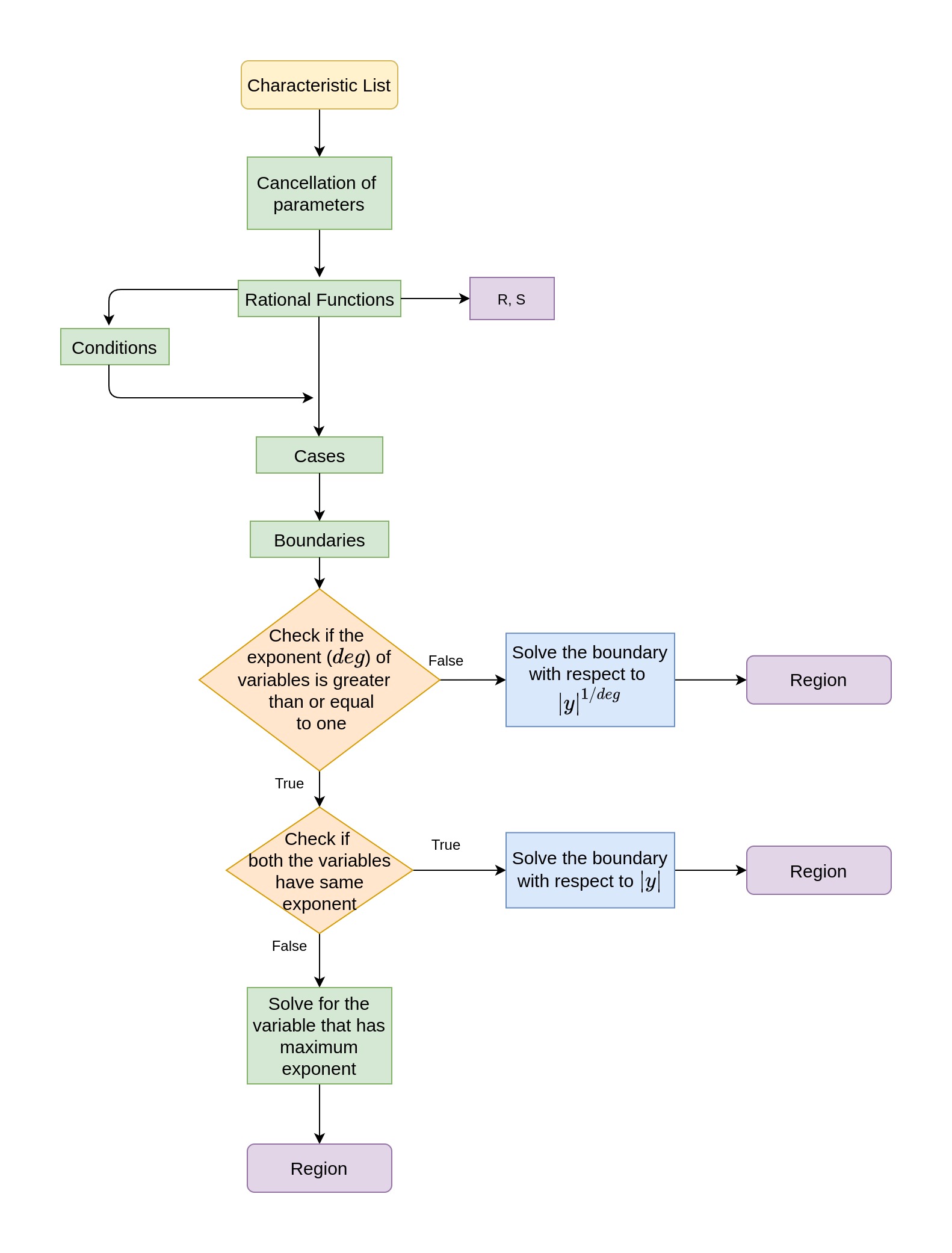
Figure 1: Flow chart of the ROC2 algorithm

The flow chart of the above algorithm is shown in figure 1. We now show how in the following section how to call the ROC2 command which applies the algorithm above.

5.1.1 Input

The algorithm of section 5.1 is implemented in the ROC2 command which takes the form

ROC2[m,n,num_List,denom_List,X,Y]

where m and n denote the two summation indices and X and Y the two variables of the studied double hypergeometric series. The two lists num_List and denom_List split the characteristic list of the series into two sets corresponding to the gamma functions appearing in the numerator and in the denominator of the series.

For example, for the $F_{2}$ series, one has

$$F_{2}(a,b_{1},b_{2},c_{1},c_{2},x,y)=\sum_{m,n=0}^{\infty}\dfrac{(a)_{m+n}(b_{1})_{m}(b_{2})_{n}}{(c_{1})_{m}(c_{2})_{n}}\dfrac{x^{m}}{m!}\dfrac{y^{n}}{n!}$$

with num_List = $\{m+n,m,n\}$, denom_List = $\{m,n\}$, X=$x$ and Y=$y$.

For the Appell $F_{3}$ series, written in terms of gamma functions,

$$F_{3}(a_{1},a_{2},b_{1},b_{2},c,x,y)=$$

$$\dfrac{\Gamma(c)}{\Gamma(a_{1})\Gamma(a_{2})\Gamma(b_{1})\Gamma(b_{2})}\sum_{m,n=0}^{\infty}\dfrac{\Gamma(a_{1}+m)\Gamma(a_{2}+m)\Gamma(b_{1}+n)\Gamma(b_{2}+n)}{\Gamma(c+m+n)}\dfrac{x^{m}}{m!}\dfrac{y^{n}}{n!}$$

one has num_List = $\{m,m,n,n\}$, denom_List = $\{m+n\}$, X=$x$ and Y=$y$.

Note that we do not include the $m!$ and $n!$ in denom_List. The order of elements in num_List and denom_List does not matter and if there is no denominator in a series then denom_List can be taken as $\{1\}$.

For the above two examples, the call of ROC2 is thus simply

$$\texttt{ROC2[m,n,\{m+n,m,n\},\{m,n\},x,y]}\hskip 28.45274pt\text{for}~{}F_{2}$$

$$\texttt{ROC2[m,n,\{m,m,n,n\},\{m+n\},x,y]}\hskip 28.45274pt\text{for}~{}F_{3}$$

One may encounter series with variables which are functions of both $x$ and $y$. The package can evaluate the ROC for those cases too. For example, the ROC of $F_{2}(a,b_{1},b_{2},c_{1},c_{2},x/y,y)$ would be obtained from ROC2[m,n,{m+n,m,n},{m,n},x/y,y].

5.1.2 Output

The output of the ROC2 command gives the rectangle $K[\rho(1,0),\sigma(0,1)]$, the Cartesian curve which will help finding the boundary of $Z$ and the ROC. If the ROC for a series is the rectangle itself then the Cartesian curve is not given. The ROC can be simplified further using the inbuilt Mathematica FullSimply command. Let us show the output for the above mentioned simple examples, before moving to a less trivial case in the next section.

     In[]:=ROC2[m, n, {m, n, m + n}, {m, n}, x, y](*ROC of F2 *)    Out[]={"{R,S}, Cartesian Curve, ROC -> ", {1,1}, {Abs[x] + Abs[y] == 1},  {Abs[x] < 1 && Abs[y] < 1 && Abs[y] < 1 - Abs[x]}}    In[]:=ROC2[m, n, {m, n, m, n}, {m + n}, x, y](*ROC of F3*)    Out[]={"{R,S}, Cartesian Curve, ROC -> ", {1,1}, {}, {Abs[x] < 1 && Abs[y] < 1}}    In[]:=ROC2[m, n, {m, n, m + n}, {m, n}, x/y, y]    Out[]={"{R,S}, Cartesian Curve, ROC -> ", {1, 1}, {Abs[x/y] + Abs[y] == 1},  {Abs[x/y] < 1 && Abs[y] < 1 && Abs[y] < 1 - Abs[x/y]}}    In[]:=FullSimplify[Last[%]](* Further simplication *)    Out[]={Abs[x/y] + Abs[y] < 1}     

5.1.3 The Horn $H_{5}$ series

In this section, we show some details about the different steps of the algorithm, when applied to the non-trivial case of the Horn $H_{5}$ series. The latter is defined as

$$H_{5}(a,b,c,x,y)=\sum_{m,n=0}^{\infty}\dfrac{(a)_{2m+n}(b)_{n-m}}{(c)_{n}}\dfrac{x^{m}}{m!}\dfrac{y^{n}}{n!}$$

Here num_List=$\{2m+n,n-m\}$, denom_List=$\{n\}$, X=$x$ and Y=$y$.
In step 1, the cancellation of parameters does not give birth to simplifications. Thus, one obtains $C(m,n)=\dfrac{(a)_{2m+n}(b)_{n-m}}{(c)_{n}}$.
In step 2, on gets the rational functions for $H_{5}$ as

$$\rho(m,n)=-\frac{m(m-n)}{(2m+n)^{2}}\hskip 28.45274pt\text{and}\hskip 28.45274pt\sigma(m,n)=\frac{n^{2}}{(n-m)(2m+n)}$$

In step 3, the rectangle is evaluated as $\rho(1,0)=\dfrac{1}{4}$ and $\sigma(0,1)=1$.
In step 4, the conditions are evaluated in terms of $t=m/n$ : $\{t>0\land t<1,t>1\}$.
In step 5, the cases are evaluated for the above conditions,

$$\Big{\{}\Big{\{}-\frac{(t-1)t}{(2t+1)^{2}},-\frac{1}{(t-1)(2t+1)}\Big{\}},\Big{\{}\frac{(t-1)t}{(2t+1)^{2}},\frac{1}{(t-1)(2t+1)}\Big{\}}\Big{\}}$$

In step 6, the boundaries are derived. There are two boundaries, one for each cases:

$$\Big{\{}\left|x\right|\left(27\left|y\right|^{2}-36\left|y\right|+8\right)+16\left|x\right|^{2}-\left|y\right|+1,-\left|x\right|\left(27\left|y\right|^{2}+36\left|y\right|+8\right)+16\left|x\right|^{2}+\left|y\right|+1\Big{\}}$$

In step 7, the degrees are found to be identical and equal to 2. The boundaries are solved for $|y|$ with the constraint $|x|<\dfrac{1}{4}$. From the first boundary one gets

$$\Big{\{}\left|y\right|=\frac{-(1-12\left|x\right|)^{3/2}+36\left|x\right|+1}{54\left|x\right|},|y|=\frac{(1-12\left|x\right|)^{3/2}+36\left|x\right|+1}{54\left|x\right|}\Big{\}}$$

and from the second

$$\Big{\{}\frac{(12\left|x\right|+1)^{3/2}+1}{\left|x\right|}=54\left|y\right|+36\Big{\}}$$

Replacing equal signs by the less than signs we find the ROC of $H_{5}$ as

$$\left|x\right|<\frac{1}{4}\land\left|y\right|<1$$

$$\land\left|y\right|<\left(\begin{array}[]{cc}\Bigg{\{}&\begin{array}[]{cc}\text{Min}\left(\frac{-(1-12\left|x\right|)^{3/2}+36\left|x\right|+1}{54\left|x\right|},\frac{(1-12\left|x\right|)^{3/2}+36\left|x\right|+1}{54\left|x\right|},\frac{(12\left|x\right|+1)^{3/2}-36\left|x\right|+1}{54\left|x\right|}\right)&\text{if}\left|x\right|<\frac{1}{12}\\ \frac{(12\left|x\right|+1)^{3/2}-36\left|x\right|+1}{54\left|x\right|}&\text{True}\\ \end{array}\\ \end{array}\right)$$

which can be checked from the code

     In[]:=ROC2[m, n, {2 m + n, n - m}, {n}, x, y]    Out[]={{R,S}, Cartesian Curve, ROC -> ,{1/4,1},  {Abs[y]==(1-(1-12 Abs[x])^(3/2)+36 Abs[x])/...}}     

5.2 Tests of ROC2.wl

We now give a comprehensive list of the known results for which the package ROC2.wl was tested. This list includes the 14 Horn’s Series $F_{1}$, …, $F_{4}$, $G_{1}$, $G_{2}$, $G_{3}$, $H_{1}$, …, $H_{7}$, seven confluent hypergeometric series and some Kampé de Fériet series.

It has to be noted that sometimes the expressions of the ROC obtained form the package can be different from the one given in literature. However, when plotted they have the same shape. For some cases the package gives results in terms of a piecewise function. Those can be written using the Minimum function in order to match with the result from the literature.

For example the ROC of $H_{5}$ found in the previous section can be conveniently written as

$$r<\frac{1}{4}\land s<1\land s<\text{min}\left[\frac{-(1-12r)^{3/2}+36r+1}{54r},\frac{(1-12r)^{3/2}+36r+1}{54r},\frac{(12r+1)^{3/2}-36r+1}{54r}\right]$$ (25)

Although both of the forms are essentially the same, the piecewise form is necessary in order to plot the ROC with Mathematica.

6 Conclusions

We have presented the package Olsson.wl, that can be used to find linear transformations for a large class of multivariable hypergeometric functions, and we have provided a tutorial on its usage.

Although the obtained analytic continuations can be viewed as functional relations, they are derived from the series representations of the multivariable hypergeometric functions under study. Due to the lack of a good knowledge of the new functions appearing in the linear transformations resulting from this procedure, the latter formulae are valid in only certain ranges of values of the arguments of these functions (the regions of convergence of the corresponding series), which in principle can be found using Horn’s theorem, allowing to solve the puzzle of the construction of the starting point function piece after piece. Still, given a multivariable hypergeometric series, finding its region of convergence can be a very difficult task. The companion package ROC2.wl provides the first automatic evaluation of regions of convergence for double hypergeometric series. Constructing algorithms and building a Mathematica package for obtaining the regions of convergence of multivariable hypergeometric series with more than 2 variables is a work in progress [29].

The analytic continuations derived from the Olsson.wl package are valid for complex values of the arguments of the involved multivariable hypergeometric series. However, the numerical evaluation of these formulae has to be done with care due to the issues of multivaluedness and branch cuts of the prefactors that appear in them. Therefore, the set of analytic continuations can be combined to built a numerical package for a general hypergeometric function only after resolving these issues. A few numerical packages are available in Mathematica and Maple for the simplest double hypergeometric functions of the Appell type, and those are far from perfect. While all the four Appell functions are implemented in Maple, only the Appell $F_{1}$ function is implemented in the kernel of Mathematica (there are also external packages for $F_{1}$ [30, 31]). The case of Appell $F_{2}$ has been recently considered by the present authors in [27] for real values of its arguments, in non logarithmic situations. We plan to built a numerical package for all the order two complete double variable hypergeometric functions and Lauricella functions in three variables, valid for complex values of their arguments, in the near future.

References

- [1] W. Becken and P. Schmelcher “The analytic continuation of the Gaussian hypergeometric function for arbitrary parameters” In Journal of Computational and Applied Mathematics 126.1, 2000, pp. 449–478 DOI: https://doi.org/10.1016/S0377-0427(00)00267-3
- [2] V. Alfaro, B. Jaksic and T. Regge “Differential properties of Feynman amplitudes” In in High-Energy Physics and Elementary Particles, 1965, pp. 263
- [3] Mikhail Kalmykov, Vladimir Bytev, Bernd A. Kniehl, Sven-Olaf Moch, Bennie F.. Ward and Scott A. Yost “Hypergeometric Functions and Feynman Diagrams” In Antidifferentiation and the Calculation of Feynman Amplitudes, 2020 arXiv:2012.14492 [hep-th]
- [4] Vladimir A. Smirnov “Analytic tools for Feynman integrals”, 2012 DOI: 10.1007/978-3-642-34886-0
- [5] B. Ananthanarayan, Sumit Banik, Samuel Friot and Shayan Ghosh “Multiple Series Representations of -fold Mellin-Barnes Integrals” In Phys. Rev. Lett. 127 American Physical Society, 2021, pp. 151601 DOI: 10.1103/PhysRevLett.127.151601
- [6] Ivan Gonzalez and Victor H. Moll “Definite integrals by the method of brackets. Part 1” In Advances in Applied Mathematics 45.1, 2010, pp. 50–73 DOI: https://doi.org/10.1016/j.aam.2009.11.003
- [7] Ivan Gonzalez, V.. Moll and Ivan Schmidt “A generalized Ramanujan Master Theorem applied to the evaluation of Feynman diagrams”, 2011 arXiv:1103.0588 [math-ph]
- [8] B. Ananthanarayan, Sumit Banik, Samuel Friot and Tanay Pathak “On the Method of Brackets”, 2021 arXiv:2112.09679 [hep-th]
- [9] “Negative dimensional integrals. I. Feynman graphs” In Physics Letters B 193.2, 1987, pp. 241–246 DOI: https://doi.org/10.1016/0370-2693(87)91229-9
- [10] Alfredo Takashi Suzuki “Massless two-loop “master” and three-loop two point function in NDIM”, 2014 arXiv:1408.4064 [math-ph]
- [11] Leonardo Cruz “Feynman integrals as A-hypergeometric functions” In JHEP 12, 2019, pp. 123 DOI: 10.1007/JHEP12(2019)123
- [12] René Pascal Klausen “Hypergeometric Series Representations of Feynman Integrals by GKZ Hypergeometric Systems” In JHEP 04, 2020, pp. 121 DOI: 10.1007/JHEP04(2020)121
- [13] Tai-Fu Feng, Chao-Hsi Chang, Jian-Bin Chen and Hai-Bin Zhang “GKZ-hypergeometric systems for Feynman integrals” In Nucl. Phys. B 953, 2020, pp. 114952 DOI: 10.1016/j.nuclphysb.2020.114952
- [14] Felix Tellander and Martin Helmer “Cohen-Macaulay Property of Feynman Integrals”, 2021 arXiv:2108.01410 [hep-th]
- [15] H Bateman “Higher Transcendental Functions” In McGraw-Hill Book Company, 1953
- [16] LJ Slater “Generalized Hypergeometric Functions” In Cambridge University Press, 1966
- [17] H Exton “Multiple hypergeometric functions and applications” In Ellis Horwood Series in Mathematics and Its Applications, 1976
- [18] H.. Srivastava and P.. Karlsson “Multiple gaussian hypergeometric series” In Ellis Horwood Series in Mathematics and Its Applications, 1985
- [19] S. I. Bezrodnykh “Horn’s hypergeometric functions with three variables” In Integral Transforms and Special Functions 32.3 Taylor & Francis, 2021, pp. 207–223 DOI: 10.1080/10652469.2020.1814770
- [20] S. I. Bezrodnykh “Analytic continuation of Lauricella’s functions , , and ” In Integral Transforms and Special Functions 31.11 Taylor & Francis, 2020, pp. 921–940 DOI: 10.1080/10652469.2020.1762081
- [21] S.. Bezrodnykh “Analytic continuation of the Lauricella function with arbitrary number of variables” In Integral Transforms and Special Functions 29.1 Taylor & Francis, 2018, pp. 21–42 DOI: 10.1080/10652469.2017.1402017
- [22] S.. Bezrodnykh “Analytic continuation of Lauricella’s function for variables close to unit near hyperplanes ” In Integral Transforms and Special Functions 0.0 Taylor & Francis, 2021, pp. 1–15 DOI: 10.1080/10652469.2021.1939329
- [23] S.. Bezrodnykh “Analytic continuation of the Horn hypergeometric series with an arbitrary number of variables” In Integral Transforms and Special Functions 31.10 Taylor & Francis, 2020, pp. 788–803 DOI: 10.1080/10652469.2020.1744590
- [24] Olsson, Per O. M. “Integration of the Partial Differential Equations for the Hypergeometric Functions and of Two and More Variables” In Journal of Mathematical Physics 5.3, 1964, pp. 420–430 DOI: 10.1063/1.1704134
- [25] A. Erdélyi “XXXIX.—Transformations of Hypergeometric Functions of Two Variables” In Proceedings of the Royal Society of Edinburgh. Section A. Mathematical and Physical Sciences 62.3 Royal Society of Edinburgh Scotland Foundation, 1948, pp. 378–385 DOI: 10.1017/S0080454100006774
- [26] H Exton “On the system of partial differential equations associated with Appell’s function ” In Journal of Physics A: Mathematical and General 28.3 IOP Publishing, 1995, pp. 631–641 DOI: 10.1088/0305-4470/28/3/017
- [27] B. Ananthanarayan, Souvik Bera, S. Friot, O. Marichev and Tanay Pathak “On the evaluation of the Appell double hypergeometric function”, 2021 arXiv:2111.05798 [math.CA]
- [28] Olsson, P. O. M. “On the integration of the differential equations of five‐parametric double‐hypergeometric functions of second order” In Journal of Mathematical Physics 18.6, 1977, pp. 1285–1294 DOI: 10.1063/1.523405
- [29] B. Ananthanarayan, Souvik Bera, S. Friot and Tanay Pathak “work in progress”
- [30] F.. Colavecchia, G. Gasaneo and J.. Miraglia “Numerical evaluation of Appell’s hypergeometric function” In Computer Physics Communications 138.1, 2001, pp. 29–43 DOI: 10.1016/S0010-4655(01)00186-2
- [31] F.. Colavecchia and G. Gasaneo “F1: A code to compute Appell’s hypergeometric function” In Computer Physics Communications 157.1, 2004, pp. 32–38 DOI: 10.1016/S0010-4655(03)00490-9