Inexact accelerated proximal gradient method with line search and reduced complexity for affine-constrained and bilinear saddle-point structured convex problems

Abstract

The goal of this paper is to reduce the total complexity of gradient-based methods for two classes of problems: affine-constrained composite convex optimization and bilinear saddle-point structured non-smooth convex optimization. Our technique is based on a double-loop inexact accelerated proximal gradient (APG) method for minimizing the summation of a non-smooth but proximable convex function and two smooth convex functions with different smoothness constants and computational costs. Compared to the standard APG method, the inexact APG method can reduce the total computation cost if one smooth component has higher computational cost but a smaller smoothness constant than the other. With this property, the inexact APG method can be applied to approximately solve the subproblems of a proximal augmented Lagrangian method for affine-constrained composite convex optimization and the smooth approximation for bilinear saddle-point structured non-smooth convex optimization, where the smooth function with a smaller smoothness constant has significantly higher computational cost. Thus it can reduce total complexity for finding an approximately optimal/stationary solution. This technique is similar to the gradient sliding technique in literature [30, 34]. The difference is that our inexact APG method can efficiently stop the inner loop by using a computable condition based on a measure of stationarity violation, while the gradient sliding methods need to pre-specify the number of iterations for the inner loop. Numerical experiments demonstrate significantly higher efficiency of our methods over an optimal primal-dual first-order method in [15] and the gradient sliding methods.

Keywords: first-order method, convex optimization, constrained optimization, saddle-point non-smooth optimization

1 Introduction

In this paper, we consider two classes of convex optimization problems: affine-constrained composite convex optimization:

(1.1) $$\min_{{\mathbf{x}}\in\mathbb{R}^{n}}~{}f({\mathbf{x}})+r({\mathbf{x}}),\mbox{ s.t. }{\mathbf{A}}{\mathbf{x}}={\mathbf{b}},\vspace{-0.2cm}$$

and bilinear saddle-point structured non-smooth optimization:

(1.2) $$\min_{{\mathbf{x}}\in\mathbb{R}^{n}}\left\{f({\mathbf{x}})+r({\mathbf{x}})+\max_{{\mathbf{y}}\in\mathbb{R}^{m}}\big{[}\langle{\mathbf{y}},{\mathbf{A}}{\mathbf{x}}\rangle-\phi({\mathbf{y}})\big{]}\right\}.\vspace{-0.2cm}$$

In both problems, $f$ is smooth convex while $r$ and $\phi$ are closed convex and admit easy proximal mappings. We further assume that $\phi$ has a bounded domain, $\nabla f$ is $L_{f}$-Lipschitz continuous, and $f$ is $\mu$-strongly convex with $\mu\geqslant 0$. For simplicity of introduction, we only consider equality constraints in (1.1) in this section, but we will consider both equality and inequality constraints in the main body of the paper as shown in (5.1).

Different from most of the existing works that target at an $\varepsilon$-optimal solution, we aim at finding $\varepsilon$-stationary solutions (defined later) of (1.1) and (1.2), which can be verified in practice more easily than the former. Moreover, we consider gradient-based methods for solving the two classes of problems. The considered methods only need to evaluate $(f,\nabla f)$ and $({\mathbf{A}}(\cdot),{\mathbf{A}}^{\top}(\cdot))$ and use the proximal mappings of $r$ and $\phi$. We are interested in the oracle complexity of the studied methods, which is defined as the numbers of queries that the methods make to $(f,\nabla f)$ and $({\mathbf{A}}(\cdot),{\mathbf{A}}^{\top}(\cdot))$, denoted by $Q_{f}$ and $Q_{{\mathbf{A}}}$ respectively, until an $\varepsilon$-stationary point is found. Additionally, we focus on a practical scenario where the cost of evaluating $(f,\nabla f)$ is significantly higher than $({\mathbf{A}}(\cdot),{\mathbf{A}}^{\top}(\cdot))$ and the proximal mappings defined by $r$ and $\phi$. This scenario arises from many applications in statistics and machine leanring, e.g., linearly constrained LASSO problems [12, 26], where evaluating $(f,\nabla f)$ requires processing a large amount of data while evaluating $({\mathbf{A}}(\cdot),{\mathbf{A}}^{\top}(\cdot))$ does not involve any data and can be relatively easy.

1.1 Composite subproblems/approximation

Although (1.1) and (1.2) have different formulations, they can be both solved by the numerical procedures that involve solving composite optimization problems with the following structure

(1.3) $$F^{*}=\min_{{\mathbf{x}}\in\mathbb{R}^{n}}\left\{F({\mathbf{x}})=g({\mathbf{x}})+H({\mathbf{x}})\right\}\text{ with }H({\mathbf{x}})=h({\mathbf{x}})+r({\mathbf{x}}),\vspace{-0.2cm}$$

where $g$ and $h$ are smooth convex, $g$ is $\mu$-strongly convex with $\mu\geqslant 0$, $\nabla g$ is $L_{g}$-Lipschitz continuous, $\nabla h$ is $L_{h}$-Lipschitz continuous, and $r$ is as in (1.1) and (1.2). Hence, reducing the complexity of solving (1.3) will lead to more efficient methods for (1.1) and (1.2). Next, we discuss the relevance of (1.3) to (1.1) and (1.2).

We consider solving (1.1) by an inexact proximal augmented Lagrangian method (iPALM), which performs the following update in the $k$th main iteration

(1.4) $${\mathbf{x}}^{(k+1)}\approx\operatorname*{arg\,min}_{{\mathbf{x}}\in\mathbb{R}^{n}}\textstyle f({\mathbf{x}})+r({\mathbf{x}})+\langle{\boldsymbol{\lambda}}^{(k)},{\mathbf{A}}{\mathbf{x}}-{\mathbf{b}}\rangle+\frac{\beta_{k}}{2}\|{\mathbf{A}}{\mathbf{x}}-{\mathbf{b}}\|^{2}+\frac{\rho_{k}}{2}\|{\mathbf{x}}-{\mathbf{x}}^{(k)}\|^{2}.\vspace{-0.2cm}$$

Here ${\mathbf{x}}^{(k)}$ is the main iterate, ${\boldsymbol{\lambda}}^{(k)}$ is the Lagrangian multiplier, $\beta_{k}>0$ is a penalty parameter and $\rho_{k}>0$ is a proximal parameter. It is easy to see that the problem in (1.4) is an instance of (1.3) with

(1.5) $$\textstyle g({\mathbf{x}})=f({\mathbf{x}})+\frac{\rho_{k}}{2}\|{\mathbf{x}}-{\mathbf{x}}^{(k)}\|^{2}\quad\text{ and }\quad h({\mathbf{x}})=\langle{\boldsymbol{\lambda}}^{(k)},{\mathbf{A}}{\mathbf{x}}-{\mathbf{b}}\rangle+\frac{\beta_{k}}{2}\|{\mathbf{A}}{\mathbf{x}}-{\mathbf{b}}\|^{2}\vspace{-0.1cm}$$

and the smoothness constants are $L_{g}=L_{f}+\rho_{k}$ and $L_{h}=\beta_{k}\|{\mathbf{A}}\|^{2}$.

For (1.2), we consider to use the smoothing technique by Nesterov [44], which approximates (1.2) by the smooth convex optimization problem

(1.6) $$\min_{{\mathbf{x}}\in\mathbb{R}^{n}}\left\{f({\mathbf{x}})+r({\mathbf{x}})+\max_{{\mathbf{y}}\in\mathbb{R}^{m}}\big{[}\textstyle\langle{\mathbf{y}},{\mathbf{A}}{\mathbf{x}}\rangle-\phi({\mathbf{y}})-\frac{\rho}{2}\|{\mathbf{y}}-{\mathbf{y}}^{(0)}\|^{2}\big{]}\right\}\vspace{-0.2cm}$$

and solves (1.6) using a smooth optimization method. Here, $\rho>0$ is a smoothing parameter, and ${\mathbf{y}}^{(0)}\in{\mathrm{dom}}(\phi)$. Again, we can view (1.6) as an instance of (1.3) with

(1.7) $$g({\mathbf{x}})=f({\mathbf{x}})\quad\text{ and }\quad h({\mathbf{x}})=\max_{{\mathbf{y}}\in\mathbb{R}^{m}}\big{[}\textstyle\langle{\mathbf{y}},{\mathbf{A}}{\mathbf{x}}\rangle-\phi({\mathbf{y}})-\frac{\rho}{2}\|{\mathbf{y}}-{\mathbf{y}}^{(0)}\|^{2}\big{]}\vspace{-0.2cm}$$

and the smoothness constants $L_{g}=L_{f}$ and $L_{h}=\|{\mathbf{A}}\|^{2}/\rho$.

1.2 Contributions

Based on these close connections between (1.1), (1.2) and (1.3), our main contribution is to show that, when the cost of evaluating $(f,\nabla f)$ is significantly higher than $({\mathbf{A}}(\cdot),{\mathbf{A}}^{\top}(\cdot))$, the complexity of solving (1.1) and (1.2) known in the literature can be further reduced if we solve (1.4) and (1.6) using an inexact accelerated proximal gradient (iAPG) method, which is a generic method for (1.3) and requires significantly fewer queries to $(f,\nabla f)$ than to $({\mathbf{A}}(\cdot),{\mathbf{A}}^{\top}(\cdot))$.

Our iAPG method is a double-loop variant of the accelerated proximal gradient (APG) method [42, 44, 58, 45, 2]. When applied to (1.3), the APG method processes the smooth component, i.e., $g+h$, as a whole and solves (1.3) by performing the following proximal gradient update in the $k$th iteration

(1.8) $${\mathbf{x}}^{(k+1)}=\operatorname*{arg\,min}\limits_{{\mathbf{x}}\in\mathbb{R}^{n}}\textstyle\left\langle\nabla g({\mathbf{y}}^{(k)})+\nabla h({\mathbf{y}}^{(k)}),{\mathbf{x}}-{\mathbf{y}}^{(k)}\right\rangle+\frac{1}{2\eta_{k}}\|{\mathbf{x}}-{\mathbf{y}}^{(k)}\|^{2}+r({\mathbf{x}}),\vspace{-0.2cm}$$

where ${\mathbf{y}}^{(k)}\in\mathbb{R}^{n}$ is an auxiliary iterate and $\eta_{k}>0$ is a step length parameter. By the assumption made on $r$, (1.8) can be solved easily, e.g., in a closed form. We denote the numbers of queries to $(g,\nabla g)$ and $(h,\nabla h)$ by $Q_{g}$ and $Q_{h}$, respectively. When $\mu>0$, it is known (see e.g., [42]) that the APG method finds an $\varepsilon$-optimal solution for (1.3) with oracle complexity $Q_{g}=Q_{h}=O\left(\sqrt{\frac{L_{g}+L_{h}}{\mu}}\log\left(\frac{1}{\varepsilon}\right)\right).$ However, according to the instantizations in (1.5) and (1.7), evaluating $(g,\nabla g)$ has significantly higher complexity than $(h,\nabla h)$ in both instances since the former requires evaluating $(f,\nabla f)$ while the latter only requires evaluating $({\mathbf{A}}(\cdot),{\mathbf{A}}^{\top}(\cdot))$. Given that, a potential strategy (see, e.g., [30, 34]) to reduce the overall complexity for solving (1.3), and thus, for solving (1.1) and (1.2) is to query $(g,\nabla g)$ and $(h,\nabla h)$ in different frequencies so as to reduce $Q_{g}$, even if doing so may slightly increase $Q_{h}$.

To implement this strategy, one technique is to separate $g$ and $h$ by solving the following proximal mapping subproblem in the $k$th iteration

(1.9) $${\mathbf{x}}^{(k+1)}=\operatorname*{arg\,min}\limits_{{\mathbf{x}}\in\mathbb{R}^{n}}\textstyle\left\langle\nabla g({\mathbf{y}}^{(k)}),{\mathbf{x}}-{\mathbf{y}}^{(k)}\right\rangle+\frac{1}{2\eta_{k}}\|{\mathbf{x}}-{\mathbf{y}}^{(k)}\|^{2}+h({\mathbf{x}})+r({\mathbf{x}}).\vspace{-0.2cm}$$

Unlike (1.8), (1.9) typically cannot be solved easily. A practical solution is to use another optimization algorithm to solve (1.9) inexactly to certain precision. This requires a double-loop implementation. Note that (1.9) is itself an instance of (1.3) and thus can be solved inexactly by the APG method in oracle complexity with logarithmic dependency on the precision thanks to the smoothness of $h$, the simplicity of $r$, and the strong convexity of $\frac{1}{2\eta_{k}}\|{\mathbf{x}}-{\mathbf{y}}^{(k)}\|^{2}$. By choosing appropriate precision for solving (1.9) in each iteration, we show that, when $\mu>0$, our iAPG method can find an $\varepsilon$-stationary solution of (1.3) with oracle complexity

(1.10) $$\textstyle Q_{g}=O\left(\sqrt{\frac{L_{g}}{\mu}}\log\left(\frac{1}{\varepsilon}\right)\right)\text{ and }Q_{h}=\tilde{O}\left(\sqrt{\frac{L_{g}+L_{h}}{\mu}}\log\left(\frac{1}{\varepsilon}\right)\right).\vspace{-0.1cm}$$

Since the evaluation of $(g,\nabla g)$ is more costly than $(h,\nabla h)$, the iAPG method can have a lower overall complexity than the APG method when $L_{h}$ is significantly larger than $L_{g}$.

According to (1.5), the iAPG method has lower complexity than the APG method for solving (1.4) when $\beta_{k}$ is much larger than $\rho_{k}$, which is exactly the case in the iPALM. As a consequence, we show that the iPALM, in which (1.4) is solved by the iAPG method, finds an $\varepsilon$-stationary point of (1.1) with oracle complexity

(1.11) $$\textstyle Q_{f}=O\left(\sqrt{\frac{L_{f}}{\mu}}\log^{2}\left(\frac{1}{\varepsilon}\right)\right)\text{ and }Q_{{\mathbf{A}}}=\tilde{O}\left(\sqrt{\frac{L_{f}}{\mu}}\log\left(\frac{1}{\varepsilon}\right)+\frac{\|{\mathbf{A}}\|}{\sqrt{\mu\varepsilon}}\right).\vspace{-0.2cm}$$

Without the affine constraint ${\mathbf{A}}{\mathbf{x}}={\mathbf{b}}$, it is shown by [41, 42] that any gradient-based method has to evaluate $(f,\nabla f)$ at least $\Omega\left(\sqrt{\frac{L_{f}}{\mu}}\log\left(\frac{1}{\varepsilon}\right)\right)$ times to find an $\varepsilon$-optimal point of (1.1). With ${\mathbf{A}}{\mathbf{x}}={\mathbf{b}}$, it is shown by [47] that any gradient-based method needs to evaluate $({\mathbf{A}}(\cdot),{\mathbf{A}}^{\top}(\cdot))$ at least $O(\frac{\|{\mathbf{A}}\|}{\sqrt{\mu\varepsilon}})$ times. In either case, the complexity of the iPALM matches the corresponding lower bound up to logarithmic factors.

Similarly, according to (1.7), the iAPG method has lower complexity than the APG method when $\rho$ is small, which is true for the smoothing method. In fact, to obtain an $\varepsilon$-optimal point of (1.2) by solving (1.6), one needs to set $\rho=\Theta(\varepsilon)$. In this case, we show that, when $\mu>0$, the smooothing method where (1.6) is solved by the iAPG method finds an $\varepsilon$-stationary point of (1.2) with the same oracle complexity as (1.11). This complexity matches the lower bound [47] up to logarithmic factors.

Summary of contributions. We summarize our contributions that are mentioned above.

• We give an iAPG method for solving (1.3). It is a double-loop method where the inner iterations are terminated using a computable stopping criterion based on the stationarity measure of the solution. This is different from existing double-loop approaches, e.g., [34, 53], which require a pre-determined total number of iterations that often depends on some unknown parameters of the problems.

• We show the oracle complexity of the proposed iAPG method, which is given in (1.10). When evaluating $(g,\nabla g)$ has significantly higher complexity than $(h,\nabla h)$ but $L_{g}$ is much smaller than $L_{h}$, the iAPG method is superior over the APG method for solving (1.3). This scenario arises in the subproblems solved during the iPALM for (1.1) and the smooth approximation of (1.2).

• Applying the iAPG method to the subproblems solved during the iPALM for (1.1), we derive the oracle complexity in (1.11) of the iPALM for finding an $\varepsilon$-stationary solution. This complexity is better than existing ones, e.g., [60, 15], when $(f,\nabla f)$ is significantly more expensive than $({\mathbf{A}}(\cdot),{\mathbf{A}}^{\top}(\cdot))$. The complexity result in [35] is similar to ours. However, the inner loop of the method in [35] requires a pre-determined number of iterations, and this often yields poor practical performance; see the experimental results in section 7. Additionally, we show that the iAPG method, in combination with the smoothing techinique by Nesterov, can find an $\varepsilon$-stationary solution of (1.2) with complexity given in (1.11) that is also better than existing ones.

1.3 Notation

We use lower-case bold letters ${\mathbf{x}},{\mathbf{y}},{\mathbf{b}},\ldots$ for vectors, ${\mathbf{1}}$ for an all-one vector/matrix of appropriate size, and upper-case bold letters ${\mathbf{A}},{\mathbf{W}},\ldots$ for matrices. ${\mathbf{x}}\odot{\mathbf{y}}$ denotes the component-wise product of ${\mathbf{x}}$ and ${\mathbf{y}}$. For any number sequence $\{a_{i}\}_{i\geqslant 0}$, we define $\sum_{i=k_{1}}^{k_{2}}a_{i}=0$ and $\prod_{i=k_{1}}^{k_{2}}a_{i}=1$ if $k_{1}>k_{2}$. The proximal mapping of a proper function $r$ is defined as ${\mathbf{prox}}_{r}\big{(}{\mathbf{z}}\big{)}:=\operatorname*{arg\,min}_{{\mathbf{x}}}\left\{\frac{1}{2}\|{\mathbf{x}}-{\mathbf{z}}\|^{2}+r({\mathbf{x}})\right\}.$

2 Literature review

The APG method [42, 44, 58, 45, 2] is an optimal gradient-based method for the composite optimization when there is no constraint and the non-smooth component in the objective function allows for an easy proximal mapping. However, the APG method cannot be directly applied to (1.1) due to the affine constraints or to (1.2) due to the sophisticated non-smooth term. The iAPG methods by [27, 53] are double-loop implementations of the APG method where the proximal gradient subproblem in each iteration is solved inexactly by another optimization algorithm. The iAPG method we studied in this paper is similar to [27, 53]. However, our method includes a line search scheme. Moreover, the inner loop in our method is terminated based on a computable stationarity measure while [53] requires a pre-determined total number of inner iterations that often depends on some unknown parameters of the problems.

The augmented Lagrangian method (ALM) [24, 51, 50] and its modern variants [17, 25, 28, 33, 29, 48, 60, 16, 52, 61, 63, 62, 18, 20, 21, 4] can be applied to (1.1). However, the methods in [17, 29] require exactly solving the ALM subproblem, i.e., (1.4) with $\rho_{k}=0$, which is not practical for many applications. Inexact ALMs are studied by [33, 48, 63] where ALM subproblems are solved inexactly by the APG method. When $\mu=0$, these methods have oracle complexity $Q_{f}=Q_{{\mathbf{A}}}=O(\frac{1}{\varepsilon})$ and, when $\mu>0$, the method by [63] has oracle complexity $Q_{f}=Q_{{\mathbf{A}}}=O(\frac{1}{\sqrt{\varepsilon}})$. An accelerated linearized ALM is studied by [60] where $f$ in (1.1) is linearized in the ALM subproblem. If the augmented term is also linearized so that the subproblem can be solved exactly, the method by [60] has the same oracle complexity as [63] in both the cases when $\mu=0$ and when $\mu>0$. If the augmented term is not linearized, the methods by [60, 4, 18, 21] only need $O(\frac{1}{\sqrt{\varepsilon}})$ iterations even when $\mu=0$, but the ALM subproblem becomes challenging to solve exactly. The linearized ALM method is analyzed in a unified framework together with other variants of the ALM by [52] and is generalized for nonlinear constraints by [62]. The same complexity as [63] is achieved in [52, 62]. A cutting-plane based ALM is proposed by [61] which can find an $\varepsilon$-KKT point for (1.1) with oracle complexity $Q_{f}=Q_{{\mathbf{A}}}=\tilde{O}(\frac{m}{\sqrt{\varepsilon}})$ when $\mu=0$ and $Q_{f}=Q_{{\mathbf{A}}}=\tilde{O}(m\log(\frac{1}{\varepsilon}))$ when $\mu>0$, where $m$ is the number of constraints. Hence, its complexity is better than ours only when $m=o(\varepsilon^{-\frac{1}{2}})$. ALM-type methods based on dynamical systems [19, 22, 5] are developed in [18, 20] which find an $\varepsilon$-solution within $o(\frac{1}{\sqrt{\varepsilon}})$ iterations if each ALM subproblem is solved exactly or inexactly with controllable errors. However, their convergence result is asymptotic, and the total oracle complexity is not given.

The (linearized) Bregman methods [67, 66] and their accelerated variants [25, 29] are equivalent to gradient-based methods applied to the Lagrangian dual problem of (1.1). Similar techniques are explored in [13, 10]. However, these methods require easy evaluation of the proximal mapping of $f$, which limits their applications. For (1.1) with a strongly convex but not necessarily smooth objective, a dual $\varepsilon$-optimal solution can be found by an accelerated Uzawa method [54] or an inexact ALM method [28] within $O(\frac{1}{\sqrt{\varepsilon}})$ main iterations. However, the method in [54] requires solving a Lagrangian subproblem exactly and is thus impractical for general $f$. Although the method by [28] only needs to solve ALM subproblems inexactly, the authors only analyze the total number of main iterations but not the overall oracle complexity.

Penalty methods [13, 10, 32, 37] are also classical approaches for (1.1), where the affine constraints are moved to the objective function through a penalty term and the unconstrained penalty problem is then solved by another optimization algorithm like the APG method. The primal method in [13, 10] requires $r=0$ and ${\mathbf{A}}$ is positive semidefinite while the dual method in [13, 10] requires an easy evaluation of the convex conjugate function of $f$, which limits the applications. When $\mu=0$, [32] shows that, if the penalty parameter is large enough, the penalty method finds an $(\varepsilon,\varepsilon)$-primal-dual solution of (1.1) (see Def. 1 in [32]) with oracle complexity $Q_{f}=Q_{{\mathbf{A}}}=O(\frac{1}{\varepsilon})$. The penalty method by [37] solves a sequence of unconstrained penalty problems with increasing penalty parameters and only performs one iteration of the APG method on each penalty problem. It has oracle complexity $Q_{f}=Q_{{\mathbf{A}}}=O(\frac{1}{\varepsilon})$ when $\mu=0$ and $Q_{f}=Q_{{\mathbf{A}}}=O(\frac{1}{\sqrt{\varepsilon}})$ when $\mu>0$. The complexity of the penalty methods in [32, 37] are higher than ours in both cases.

Using Lagrangian multipliers, a constrained optimization problem can be formulated as a min-max problem to which the primal-dual methods [55, 56, 57, 68, 59], mostly based on smoothing technique [44], can be applied. However, the methods by [55, 59, 57] require a closed-form solution of the proximal mapping of $f$ while the method by [68] requires a closed-form solution of the convex conjugate function of $f$, and thus they have limited applications. The authors of [56] extend the algorithm and analysis in [55] by allowing the proximal mapping of $f$ to be evaluated inexactly. However, they do not include the oracle complexity for inexactly evaluating the proximal mapping in their complexity analysis.

Smoothing techniques [44, 3, 1] are a class of effective approaches for solving the structured non-smooth problem (1.2). These methods construct close approximation of (1.2) by one or a sequence of smooth problems, which are then solved by smooth optimization methods such as the APG method. When $\mu=0$, the methods by [44, 3, 1] find an $\varepsilon$-optimal solution with complexity $Q_{f}=Q_{{\mathbf{A}}}=O(\frac{\|A\|}{\varepsilon}+\sqrt{\frac{L_{f}}{\varepsilon}})$. When $\mu>0$, the adapative smoothing method by [1] finds an $\varepsilon$-optimal solution with complexity $Q_{f}=Q_{{\mathbf{A}}}=O(\sqrt{\frac{L_{f}}{\mu}}\log(\frac{1}{\varepsilon})+\frac{\|A\|}{\sqrt{\mu\varepsilon}})$, which is higher than our complexity given in (1.11) when the query to $(f,\nabla f)$ is significantly more costly than $({\mathbf{A}}(\cdot),{\mathbf{A}}^{\top}(\cdot))$.

In the literature, (1.2) has also been studied as a bilinear saddle point problem [6, 7, 8, 23, 43, 69, 70]. The methods in [6, 7, 43] require a closed form of the proximal mapping of $f+r$ and thus may not be applicable to (1.2). When $\mu=0$, the methods by [23, 8, 69, 70] find an $\varepsilon$-saddle-point (see Def. 3.1 in [23]) or an $\varepsilon$-optimal solution with the same oracle complexity as the smoothing methods mentioned above. When $\mu>0$, the method by [70] finds an $\varepsilon$-optimal solution with the same oracle complexity as the smoothing method [1]. Problem (1.2) has also been studied as a variational inequality [40, 9, 58]. In particular, when $\mu=0$, the mirror-prox methods in [40, 58] find an $\varepsilon$-optimal solution of (1.2) with complexity $Q_{f}=Q_{{\mathbf{A}}}=O(\frac{L_{f}+\|A\|}{\varepsilon})$, which is later reduced to $Q_{f}=Q_{{\mathbf{A}}}=O(\sqrt{\frac{L_{f}}{\varepsilon}}+\frac{\|A\|}{\varepsilon})$ by [9].

For all the methods we discussed above for solving (1.1) and (1.2), the oracle complexity is essentially the number of iterations the algorithms perform to find the desired solution. Since all of those methods always evaluate both $(f,\nabla f)$ and $({\mathbf{A}}(\cdot),{\mathbf{A}}^{\top}(\cdot))$ in each iteration, $Q_{f}$ and $Q_{{\mathbf{A}}}$ are the same for them. When the evaluation cost of $(f,\nabla f)$ is significantly higher than that of $({\mathbf{A}}(\cdot),{\mathbf{A}}^{\top}(\cdot))$, it will be more efficient to query $(f,\nabla f)$ less frequently than $({\mathbf{A}}(\cdot),{\mathbf{A}}^{\top}(\cdot))$ without compromising the solution quality. This actually can be achieved using the gradient sliding techniques [30, 34, 36, 31, 46], which compute the gradient of one (more expensive) component of the objective function once in each outer iteration and process the remaining components in each inner iteration. The iAPG method in this paper utilizes a similar double-loop technique to differentiate the frequencies of evaluating $(f,\nabla f)$ and $({\mathbf{A}}(\cdot),{\mathbf{A}}^{\top}(\cdot))$ and thus reduce $Q_{f}$. Although the idea behind the iAPG method is similar to the gradient sliding techniques, such a technique has not be studied for problem (1.1) under an iPALM framework. Although (1.2) has been studied by [30, 34], we consider the case of $\mu>0$, which is not covered in [30] and for which [34] needs to apply the sliding method for convex cases in multiple stages. Moreover, in the existing works on the gradient sliding techniques, the inner loop must run for a pre-determined number of iterations which depends on some unknown parameters of the problems. On the contrary, we terminate our inner loop based on a computable stationarity measure, which makes our method more efficient in practice as we demonstrate in Section 7.

3 Inexact Accelerated Proximal Gradient Method with Line Search

In this section, we consider (1.3) where $g$ is $\mu$-strongly convex with $\mu\geqslant 0$ and $L_{g}$-smooth (i.e. $\nabla g$ is $L_{g}$-Lipschitz continuous), $h$ are convex and $L_{h}$-smooth, and $r$ is closed convex and allows easy computation of ${\mathbf{prox}}_{\eta r}\big{(}{\mathbf{z}}\big{)}$ for any ${\mathbf{z}}\in\mathbb{R}^{n}$ and $\eta>0$. We assume that $(g,\nabla g)$ is significantly more costly to evaluate than $(h,\nabla h)$ and $L_{g}$ is significantly smaller than $L_{h}$. To have a low overall complexity, we propose an iAPG method that calls $(g,\nabla g)$ less frequently than $(h,\nabla h)$. It is given in Algorithm 1. This algorithm is a modification of the APG method in [42, Algorithm 2.2.19] by including a line search procedure (in Algorithm 2) for the step length parameter $\eta_{k}$ and solving the following proximal mapping subproblem inexactly

(3.1) $$\textstyle{\mathbf{x}}^{(k+1)}\approx{\mathbf{x}}^{(k+1)}_{*}:=\operatorname*{arg\,min}\limits_{{\mathbf{x}}\in\mathbb{R}^{n}}\left\{\Phi({\mathbf{x}};{\mathbf{y}}^{(k)},\eta_{k}):=\left\langle\nabla g({\mathbf{y}}^{(k)}),{\mathbf{x}}-{\mathbf{y}}^{(k)}\right\rangle+\frac{1}{2\eta_{k}}\|{\mathbf{x}}-{\mathbf{y}}^{(k)}\|^{2}+h({\mathbf{x}})+r({\mathbf{x}})\right\}.\vspace{-0.2cm}$$

Compared to the APG method that requires ${\mathbf{x}}^{(k+1)}={\mathbf{x}}^{(k+1)}_{*}$, our iAPG method only needs ${\mathbf{x}}^{(k+1)}$ to be an $\varepsilon_{k}$-stationary point, namely, a point satisfying the inequality (3.2). Our line search procedure follows that in [39] for the APG method on solving strongly convex problems.

It can be shown that ${\mathbf{x}}^{(k+1)}$ produced by the iAPG method is an $\varepsilon$-optimal solution of (1.3) if $k$ is large enough and $\varepsilon_{k}$ is small enough. However, we are more interested in finding an $\varepsilon$-stationary solution of (1.3). For this purpose, we just need to perform a proximal gradient step from ${\mathbf{x}}^{(k+1)}$ using a step length $\tilde{\eta}_{k}$ that is potentially different from $\eta_{k}$ and can also be searched by the standard scheme as in [2]. We present the optional procedure to generate an $\varepsilon$-stationary solution from the iAPG method in Algorithm 3.

1 Inputs: ${\mathbf{z}}^{(0)}={\mathbf{x}}^{(0)}\in{\mathrm{dom}}(H)$, $\eta_{-1}\leqslant\frac{1}{\mu}$, $\gamma_{0}\in\left\{\begin{array}[]{ll}(0,1/\eta_{-1}]&\text{ if }\mu=0\\ \text{[}\mu,1/\eta_{-1}]&\text{ if }\mu>0\end{array}\right.$, $\mu\leqslant\underline{L}\in(0,L_{g}]$, and $\varepsilon_{k}\geqslant 0,\forall\,k$

2 Optional: choose $\tilde{\eta}_{0}\leqslant\frac{1}{\underline{L}}$ and $\varepsilon\geqslant 0$

3 for $k=0,1,\ldots,$ do

4       Generate $({\mathbf{x}}^{(k+1)},{\mathbf{y}}^{(k)},\gamma_{k+1},\eta_{k},\alpha_{k})=\text{InexactAccelLineSearch}({\mathbf{x}}^{(k)},{\mathbf{z}}^{(k)},\gamma_{k},\eta_{k-1},\mu,\underline{L},\varepsilon_{k})$

5       ${\mathbf{z}}^{(k+1)}={\mathbf{x}}^{(k)}+\frac{1}{\alpha_{k}}\left({\mathbf{x}}^{(k+1)}-{\mathbf{x}}^{(k)}\right)$

6       Optional: $(\widetilde{\mathbf{x}}^{(k+1)},\tilde{\eta}_{k+1})=\text{SeekStationary}({\mathbf{x}}^{(k+1)},\tilde{\eta}_{k})$

7       Optional: Return $\widetilde{\mathbf{x}}^{(k+1)}$ if $\mathrm{dist}\big{(}\mathbf{0},\partial F(\widetilde{\mathbf{x}}^{(k+1)})\big{)}\leqslant\varepsilon$

Algorithm 1 $\mathrm{iAPG}(g,h,r,{\mathbf{x}}^{(0)},\eta_{-1},\gamma_{0},\mu,\underline{L},(\varepsilon_{k})_{k\geqslant 0})$ for solving (1.3)

1 Parameters: $\gamma_{\mathrm{dec}}\in(0,1)$ and $\gamma_{\mathrm{inc}}\in[1,+\infty)$

2 $\eta_{k}\leftarrow\min\big{\{}\frac{1}{\gamma_{\mathrm{dec}}\underline{L}},\ \gamma_{\mathrm{inc}}\eta_{k-1}\big{\}}$

3 repeat

4       $\eta_{k}\leftarrow\gamma_{\mathrm{dec}}\eta_{k}$; find $\alpha_{k}>0$ and $\gamma_{k+1}$ that satisfy $\gamma_{k+1}=\frac{\alpha_{k}^{2}}{\eta_{k}}=\left(1-\alpha_{k}\right)\gamma_{k}+\alpha_{k}\mu$

5       Let ${\mathbf{y}}^{(k)}=\frac{1}{\alpha_{k}\gamma_{k}+\gamma_{k+1}}\left(\alpha_{k}\gamma_{k}{\mathbf{z}}^{(k)}+\gamma_{k+1}{\mathbf{x}}^{(k)}\right)$

6       Find ${\mathbf{x}}^{(k+1)}$ such that

(3.2) $$\textstyle\mathrm{dist}\left(\mathbf{0},\nabla g({\mathbf{y}}^{(k)})+\frac{1}{\eta_{k}}({\mathbf{x}}^{(k+1)}-{\mathbf{y}}^{(k)})+\partial H({\mathbf{x}}^{(k+1)})\right)\leqslant\varepsilon_{k}\vspace{-0.1cm}$$

7until $g({\mathbf{x}}^{(k+1)})\leqslant g({\mathbf{y}}^{(k)})+\langle\nabla g({\mathbf{y}}^{(k)}),{\mathbf{x}}^{(k+1)}-{\mathbf{y}}^{(k)}\rangle+\frac{1}{2\eta_{k}}\|{\mathbf{x}}^{(k+1)}-{\mathbf{y}}^{(k)}\|^{2}$

Return: $({\mathbf{x}}^{(k+1)},{\mathbf{y}}^{(k)},\gamma_{k+1},\eta_{k},\alpha_{k})$

Algorithm 2 $({\mathbf{x}}^{(k+1)},{\mathbf{y}}^{(k)},\gamma_{k+1},\eta_{k},\alpha_{k})=\text{InexactAccelLineSearch}({\mathbf{x}}^{(k)},{\mathbf{z}}^{(k)},\gamma_{k},\eta_{k-1},\mu,\underline{L},\varepsilon_{k})$

1 $\tilde{\eta}\leftarrow\eta/\gamma_{\mathrm{dec}}$ with the same $\gamma_{\mathrm{dec}}\in(0,1)$ as that in Algorithm 2

2 repeat

3       $\tilde{\eta}\leftarrow\gamma_{\mathrm{dec}}\tilde{\eta}$ and let $\widetilde{\mathbf{x}}={\mathbf{prox}}_{\tilde{\eta}r}\big{(}{\mathbf{x}}-\tilde{\eta}(\nabla g({\mathbf{x}})+\nabla h({\mathbf{x}}))\big{)}$.

4until $g(\widetilde{\mathbf{x}})+h(\widetilde{\mathbf{x}})\leqslant g({\mathbf{x}})+h({\mathbf{x}})+\left\langle\nabla g({\mathbf{x}})+\nabla h({\mathbf{x}}),\widetilde{\mathbf{x}}-{\mathbf{x}}\right\rangle+\frac{1}{2\tilde{\eta}}\|\widetilde{\mathbf{x}}-{\mathbf{x}}\|^{2}$

Return: $\tilde{\eta}$.

Algorithm 3 $(\widetilde{\mathbf{x}},\tilde{\eta})=\text{SeekStationary}({\mathbf{x}},\eta)$

3.1 Convergence analysis for iAPG

In this subsection, we analyze the convergence rate of the proposed iAPG. The analysis also applies to APG by setting $\varepsilon_{k}=0$. The technical lemmas below are needed.

Lemma 1.

Let $(\eta_{k},\tilde{\eta}_{k},\alpha_{k},\gamma_{k})$ be generated from Algorithm 1. It holds that, for any $k\geqslant 0$,

(3.3) $$\textstyle\frac{\gamma_{\mathrm{dec}}}{L_{g}}<\eta_{k}\leqslant\frac{1}{\underline{L}},~{}\frac{\gamma_{\mathrm{dec}}}{L_{g}+L_{h}}<\tilde{\eta}_{k}\leqslant\frac{1}{\underline{L}},~{}\alpha_{k}\leqslant 1~{}\text{and}~{}\gamma_{k}\geqslant\mu.\vspace{-0.3cm}$$

Proof. From Lines 2 and 4 of Algorithm 2, we must have $\eta_{k}\leqslant\frac{1}{\underline{L}}$ for $k\geqslant 0$ in Algorithm 1. In addition, the condition in Line 7 of Algorithm 2 will hold and Algorithm 2 will stop if $\eta_{k}\leqslant\frac{1}{L_{g}}$. Given Line 4 of Algorithm 2, we must have $\eta_{k}>\frac{\gamma_{\mathrm{dec}}}{L_{g}}$ in Algorithm 1. By the same arguments, we can prove $\frac{\gamma_{\mathrm{dec}}}{L_{g}+L_{h}}<\tilde{\eta}_{k}\leqslant\frac{1}{\underline{L}}$.

Now solving $\alpha_{k}$ from equation $\frac{\alpha_{k}^{2}}{\eta_{k}}=\left(1-\alpha_{k}\right)\gamma_{k}+\alpha_{k}\mu$ in Line 4 of Algorithm 2, we have

(3.4) $$\textstyle\alpha_{k}=\frac{-(\gamma_{k}-\mu)+\sqrt{(\gamma_{k}-\mu)^{2}+4\gamma_{k}/\eta_{k}}}{2/\eta_{k}}=\frac{2\gamma_{k}}{(\gamma_{k}-\mu)+\sqrt{(\gamma_{k}-\mu)^{2}+4\gamma_{k}/\eta_{k}}}.\vspace{-0.1cm}$$

Since $\mu\leqslant\underline{L}\leqslant 1/\eta_{k}$, we have $(\gamma_{k}-\mu)^{2}+4\gamma_{k}/\eta_{k}\geqslant(\gamma_{k}+\mu)^{2}$. Thus it follows from (3.4) that $\alpha_{k}\leqslant 1,\forall\,k\geqslant 0$. Notice if $\gamma_{k}\geqslant\mu$, then $\gamma_{k+1}=\left(1-\alpha_{k}\right)\gamma_{k}+\alpha_{k}\mu\geqslant\mu$. Since $\gamma_{0}\geqslant\mu$, we have $\gamma_{k}\geqslant\mu,\forall\,k\geqslant 0$ by induction. $\Box$

Lemma 2.

In any iteration of Algorithm 1, Algorithm 2 and Algorithm 3 will perform at most $\lceil\log_{\gamma_{\mathrm{dec}}}\frac{\underline{L}}{L_{g}}\rceil$ and $\lceil\log_{\gamma_{\mathrm{dec}}}\frac{\underline{L}}{L_{g}+L_{h}}\rceil$ iterations, respectively. Moreover, if Algorithm 1 runs for $t$ iterations, Algorithm 2 and Algorithm 3 will perform at most $\left(\frac{\log\gamma_{\mathrm{inc}}}{\log\gamma^{-1}_{\mathrm{dec}}}\right)(t-1)+\frac{1}{\log\gamma^{-1}_{\mathrm{dec}}}\min\left\{\log\left(\frac{L_{g}}{\gamma^{2}_{\mathrm{dec}}\underline{L}}\right),\ \log\left(\frac{\gamma_{\mathrm{inc}}\eta_{-1}L_{g}}{\gamma_{\mathrm{dec}}}\right)\right\}$ and $t+1+\frac{1}{\log\gamma^{-1}_{\mathrm{dec}}}\log\left(\frac{L_{g}+L_{h}}{\underline{L}}\right)$ iterations in total, respectively.

Proof. The first conclusion is from (3.3). The second one can be proved similarly as Lemma 6 in [45]. $\Box$

Lemma 3.

Let $\tau=\frac{L_{g}}{\gamma_{\mathrm{dec}}\underline{L}},\ \kappa=\frac{L_{g}}{\gamma_{\mathrm{dec}}\mu}$ and $\alpha_{k}$ be generated by Algorithm 1. It holds that, for $k\geqslant 0$,

(3.5) $$\textstyle\frac{1}{(k+1/\alpha_{0})\sqrt{\tau}}\leqslant\alpha_{k}\leqslant\frac{2\sqrt{\tau}}{k+2},\text{ if }\mu=0;\quad\sqrt{\frac{1}{\kappa}}\leqslant\alpha_{k},\text{ if }\mu>0,\vspace{-0.2cm}$$

Proof. When $\mu=0$, Line 4 of Algorithm 2 implies $\frac{\alpha_{k}^{2}}{\eta_{k}}=(1-\alpha_{k})\gamma_{k}=(1-\alpha_{k})\frac{\alpha_{k-1}^{2}}{\eta_{k-1}}$, and thus $\frac{1}{\alpha_{k}^{2}}-\frac{1}{\alpha_{k}}=\frac{1}{\alpha_{k-1}^{2}}\frac{\eta_{k-1}}{\eta_{k}}$ for $k\geqslant 1$ in Algorithm 1. By the quadratic formula, it follows that

(3.6) $$\textstyle\frac{1}{\alpha_{k}}=\frac{1+\sqrt{1+\frac{4}{\alpha_{k-1}^{2}}\frac{\eta_{k-1}}{\eta_{k}}}}{2}\geqslant\frac{1}{2}+\frac{1}{\alpha_{k-1}}\sqrt{\frac{\eta_{k-1}}{\eta_{k}}}.\vspace{-0.1cm}$$

Recursively applying (3.6) gives

(3.7) $$\textstyle\frac{1}{\alpha_{k}}\geqslant\frac{1}{2}\left(1+\sqrt{\frac{\eta_{k-1}}{\eta_{k}}}\right)+\frac{1}{\alpha_{k-2}}\sqrt{\frac{\eta_{k-2}}{\eta_{k}}}\geqslant\ldots\geqslant\frac{1}{2}\sum_{j=1}^{k}\sqrt{\frac{\eta_{j}}{\eta_{k}}}+\frac{1}{\alpha_{0}}\sqrt{\frac{\eta_{0}}{\eta_{k}}}.\vspace{-0.1cm}$$

According to (3.3), it holds that $\frac{\eta_{j}}{\eta_{k}}>\frac{1}{\tau}$ for $k$ and $j\geqslant 0$, and thus (3.7) implies $\textstyle\frac{1}{\alpha_{k}}\geqslant\big{(}\frac{k}{2}+\frac{1}{\alpha_{0}}\big{)}\sqrt{\frac{1}{\tau}}\geqslant\frac{k+2}{2}\sqrt{\frac{1}{\tau}},$ where the second inequality is because $\alpha_{0}\leqslant 1$ by Lemma 1. In addition, from the equality in (3.6) and the fact that $\sqrt{a+b}\leqslant\sqrt{a}+\sqrt{b}$, we have $\textstyle\frac{1}{\alpha_{k}}\leqslant 1+\frac{1}{\alpha_{k-1}}\sqrt{\frac{\eta_{k-1}}{\eta_{k}}}$. Recursively applying this inequality gives

(3.8) $$\textstyle\frac{1}{\alpha_{k}}\leqslant\left(1+\sqrt{\frac{\eta_{k-1}}{\eta_{k}}}\right)+\frac{1}{\alpha_{k-2}}\sqrt{\frac{\eta_{k-2}}{\eta_{k}}}\leqslant\ldots\leqslant\sum_{j=1}^{k}\sqrt{\frac{\eta_{j}}{\eta_{k}}}+\frac{1}{\alpha_{0}}\sqrt{\frac{\eta_{0}}{\eta_{k}}}.\vspace{-0.1cm}$$

By (3.3) again, we have $\frac{\eta_{j}}{\eta_{k}}<{\tau}$ for all $k$ and $j\geqslant 0$, and thus (3.8) implies $\textstyle\frac{1}{\alpha_{k}}\leqslant\big{(}k+\frac{1}{\alpha_{0}}\big{)}\sqrt{\tau}.$

When $\mu>0$, we have from Lemma 1 that $\gamma_{k+1}\geqslant\mu$. Hence, from (3.3) and the updating equation of $\gamma_{k+1}$, it follows that $\alpha_{k}=\sqrt{\eta_{k}\gamma_{k+1}}\geqslant\sqrt{\frac{1}{\kappa}}$. Therefore, we obtain the desired results. $\Box$

Next, we establish the relationship between two consecutive iterates in Algorithm 1.

Proposition 4.

Let $\{({\mathbf{x}}^{(k)},{\mathbf{z}}^{(k)},\alpha_{k},\gamma_{k})\}$ be generated by Algorithm 1. It holds that, for $k\geqslant 0$,

(3.9) $$\textstyle F({\mathbf{x}}^{(k+1)})-F^{*}+\frac{\gamma_{k+1}}{2}\|{\mathbf{x}}^{*}-{\mathbf{z}}^{(k+1)}\|^{2}\leqslant(1-\alpha_{k})\left[F({\mathbf{x}}^{(k)})-F^{*}+\frac{\gamma_{k}}{2}\|{\mathbf{x}}^{*}-{\mathbf{z}}^{(k)}\|^{2}\right]+\varepsilon_{k}\alpha_{k}\|{\mathbf{x}}^{*}-{\mathbf{z}}^{(k+1)}\|.\vspace{-0.1cm}$$

Proof. Let ${\mathbf{x}}^{*}$ be an optimal solution of (1.3) and define $\widehat{\mathbf{x}}^{(k)}=\alpha_{k}{\mathbf{x}}^{*}+(1-\alpha_{k}){\mathbf{x}}^{(k)}\in{\mathrm{dom}}(H)$. Then

(3.10) $$\widehat{\mathbf{x}}^{(k)}-{\mathbf{y}}^{(k)} = \alpha_{k}({\mathbf{x}}^{*}-{\mathbf{y}}^{(k)})+(1-\alpha_{k})({\mathbf{x}}^{(k)}-{\mathbf{y}}^{(k)}).$$

By the updating equation of ${\mathbf{y}}^{(k)}$ in Line 5 of Algorithm 2, it holds that ${\mathbf{z}}^{(k)}-{\mathbf{y}}^{(k)}=-\frac{\gamma_{k+1}}{\alpha_{k}\gamma_{k}}\left({\mathbf{x}}^{(k)}-{\mathbf{y}}^{(k)}\right)$. This together with (3.10) gives

(3.11) $$\widehat{\mathbf{x}}^{(k)}-{\mathbf{y}}^{(k)} = \textstyle\alpha_{k}({\mathbf{x}}^{*}-{\mathbf{y}}^{(k)})-\frac{\alpha_{k}(1-\alpha_{k})\gamma_{k}}{\gamma_{k+1}}({\mathbf{z}}^{(k)}-{\mathbf{y}}^{(k)})=\alpha_{k}\left[{\mathbf{x}}^{*}-{\mathbf{y}}^{(k)}-\frac{(1-\alpha_{k})\gamma_{k}}{\gamma_{k+1}}({\mathbf{z}}^{(k)}-{\mathbf{y}}^{(k)})\right]$$

$$= \textstyle\alpha_{k}\left[{\mathbf{x}}^{*}-\frac{(1-\alpha_{k})\gamma_{k}}{\gamma_{k+1}}{\mathbf{z}}^{(k)}-\frac{\alpha_{k}\mu}{\gamma_{k+1}}{\mathbf{y}}^{(k)}\right],\vspace{-0.1cm}$$

where the last equality follows from the updating equation of $\gamma_{k+1}$.

According to (3.2), there exists ${\mathbf{e}}^{(k)}\in\mathbb{R}^{n}$ such that $\|{\mathbf{e}}^{(k)}\|\leqslant\varepsilon_{k}$ and ${\mathbf{e}}^{(k)}-\nabla g({\mathbf{y}}^{(k)})-\frac{1}{\eta_{k}}({\mathbf{x}}^{(k+1)}-{\mathbf{y}}^{(k)})\in\partial H({\mathbf{x}}^{(k+1)})$. By the convexity of $H$, we have

$$H({\mathbf{x}}^{(k+1)})\leqslant ~{}\textstyle H(\widehat{\mathbf{x}}^{(k)})+\big{\langle}{\mathbf{e}}^{(k)}-\nabla g({\mathbf{y}}^{(k)})-\frac{1}{\eta_{k}}({\mathbf{x}}^{(k+1)}-{\mathbf{y}}^{(k)}),{\mathbf{x}}^{(k+1)}-\widehat{\mathbf{x}}^{(k)}\big{\rangle},\vspace{-0.1cm}$$

which, by the fact that $\langle{\mathbf{u}},{\mathbf{v}}\rangle=\frac{1}{2}\big{(}\|{\mathbf{u}}\|^{2}+\|{\mathbf{v}}\|^{2}-\|{\mathbf{u}}-{\mathbf{v}}\|^{2}\big{)}$, implies

$$H({\mathbf{x}}^{(k+1)})\leqslant ~{}\textstyle H(\widehat{\mathbf{x}}^{(k)})+\left\langle{\mathbf{e}}^{(k)}-\nabla g({\mathbf{y}}^{(k)}),{\mathbf{x}}^{(k+1)}-\widehat{\mathbf{x}}^{(k)}\right\rangle$$

$$~{}\textstyle-\frac{1}{2\eta_{k}}\left(\|{\mathbf{x}}^{(k+1)}-{\mathbf{y}}^{(k)}\|^{2}+\|{\mathbf{x}}^{(k+1)}-\widehat{\mathbf{x}}^{(k)}\|^{2}-\|\widehat{\mathbf{x}}^{(k)}-{\mathbf{y}}^{(k)}\|^{2}\right),$$

$$\leqslant ~{}\textstyle H(\widehat{\mathbf{x}}^{(k)})+\left\langle\nabla g({\mathbf{y}}^{(k)}),\widehat{\mathbf{x}}^{(k)}-{\mathbf{x}}^{(k+1)}\right\rangle+\varepsilon_{k}\|{\mathbf{x}}^{(k+1)}-\widehat{\mathbf{x}}^{(k)}\|$$

$$~{}\textstyle-\frac{1}{2\eta_{k}}\left(\|{\mathbf{x}}^{(k+1)}-{\mathbf{y}}^{(k)}\|^{2}+\|{\mathbf{x}}^{(k+1)}-\widehat{\mathbf{x}}^{(k)}\|^{2}-\|\widehat{\mathbf{x}}^{(k)}-{\mathbf{y}}^{(k)}\|^{2}\right).\vspace{-0.1cm}$$

From the inequality above and the stopping condition of Algorithm 2, we have

$$F({\mathbf{x}}^{(k+1)}) \leqslant \textstyle g({\mathbf{y}}^{(k)})+\big{\langle}\nabla g({\mathbf{y}}^{(k)}),{\mathbf{x}}^{(k+1)}-{\mathbf{y}}^{(k)}\big{\rangle}+\frac{1}{2\eta_{k}}\big{\|}{\mathbf{x}}^{(k+1)}-{\mathbf{y}}^{(k)}\big{\|}^{2}+H({\mathbf{x}}^{(k+1)})$$

$$\leqslant \textstyle g({\mathbf{y}}^{(k)})+\big{\langle}\nabla g({\mathbf{y}}^{(k)}),\widehat{\mathbf{x}}^{(k)}-{\mathbf{y}}^{(k)}\big{\rangle}+\frac{1}{2\eta_{k}}\big{\|}\widehat{\mathbf{x}}^{(k)}-{\mathbf{y}}^{(k)}\big{\|}^{2}+H(\widehat{\mathbf{x}}^{(k)})-\frac{1}{2\eta_{k}}\big{\|}\widehat{\mathbf{x}}^{(k)}-{\mathbf{x}}^{(k+1)}\big{\|}^{2}$$

$$+\varepsilon_{k}\|{\mathbf{x}}^{(k+1)}-\widehat{\mathbf{x}}^{(k)}\|.$$

Applying (3.10) to the above inequality, we have

$$F({\mathbf{x}}^{(k+1)}) \leqslant g({\mathbf{y}}^{(k)})+\big{\langle}\nabla g({\mathbf{y}}^{(k)}),\alpha_{k}({\mathbf{x}}^{*}-{\mathbf{y}}^{(k)})+(1-\alpha_{k})({\mathbf{x}}^{(k)}-{\mathbf{y}}^{(k)})\big{\rangle}$$

$$\textstyle+\frac{1}{2\eta_{k}}\big{\|}\widehat{\mathbf{x}}^{(k)}-{\mathbf{y}}^{(k)}\big{\|}^{2}+H(\alpha_{k}{\mathbf{x}}^{*}+(1-\alpha_{k}){\mathbf{x}}^{(k)})-\frac{1}{2\eta_{k}}\big{\|}\widehat{\mathbf{x}}^{(k)}-{\mathbf{x}}^{(k+1)}\big{\|}^{2}+\varepsilon_{k}\|{\mathbf{x}}^{(k+1)}-\widehat{\mathbf{x}}^{(k)}\|.\vspace{-0.1cm}$$

By the fact that $\alpha_{k}\in(0,1]$ from Lemma 1, (3.11) and the convexity of $H$, we have

$$F({\mathbf{x}}^{(k+1)}) \leqslant (1-\alpha_{k})\big{[}g({\mathbf{y}}^{(k)})+\langle\nabla g({\mathbf{y}}^{(k)}),{\mathbf{x}}^{(k)}-{\mathbf{y}}^{(k)}\rangle+H({\mathbf{x}}^{(k)})\big{]}$$

$$+\alpha_{k}\big{[}g({\mathbf{y}}^{(k)})+\left\langle\nabla g({\mathbf{y}}^{(k)}),{\mathbf{x}}^{*}-{\mathbf{y}}^{(k)}\right\rangle+H({\mathbf{x}}^{*})\big{]}$$

$$\textstyle+\frac{\alpha_{k}^{2}}{2\eta_{k}}\big{\|}{\mathbf{x}}^{*}-\frac{(1-\alpha_{k})\gamma_{k}}{\gamma_{k+1}}{\mathbf{z}}^{(k)}-\frac{\alpha_{k}\mu}{\gamma_{k+1}}{\mathbf{y}}^{(k)}\big{\|}^{2}-\frac{1}{2\eta_{k}}\big{\|}\widehat{\mathbf{x}}^{(k)}-{\mathbf{x}}^{(k+1)}\big{\|}^{2}+\varepsilon_{k}\|{\mathbf{x}}^{(k+1)}-\widehat{\mathbf{x}}^{(k)}\|.\vspace{-0.1cm}$$

Since $\gamma_{k+1}=\alpha^{2}_{k}/\eta_{k}=\left(1-\alpha_{k}\right)\gamma_{k}+\alpha_{k}\mu$, we have from the convexity of $\|\cdot\|^{2}$ that

$$\textstyle\frac{\alpha_{k}^{2}}{2\eta_{k}}\big{\|}{\mathbf{x}}^{*}-\frac{(1-\alpha_{k})\gamma_{k}}{\gamma_{k+1}}{\mathbf{z}}^{(k)}-\frac{\alpha_{k}\mu}{\gamma_{k+1}}{\mathbf{y}}^{(k)}\big{\|}^{2} = \textstyle\frac{\gamma_{k+1}}{2}\big{\|}{\mathbf{x}}^{*}-\frac{(1-\alpha_{k})\gamma_{k}}{\gamma_{k+1}}{\mathbf{z}}^{(k)}-\frac{\alpha_{k}\mu}{\gamma_{k+1}}{\mathbf{y}}^{(k)}\big{\|}^{2}$$

$$\leqslant \textstyle\frac{(1-\alpha_{k})\gamma_{k}}{2}\|{\mathbf{x}}^{*}-{\mathbf{z}}^{(k)}\|^{2}+\frac{\alpha_{k}\mu}{2}\|{\mathbf{x}}^{*}-{\mathbf{y}}^{(k)}\|^{2},\vspace{-0.2cm}$$

which, together with (3.1) and the $\mu$-strong convexity of $g$, implies

(3.14) $$F({\mathbf{x}}^{(k+1)}) \leqslant \textstyle(1-\alpha_{k})\big{[}g({\mathbf{y}}^{(k)})+\langle\nabla g({\mathbf{y}}^{(k)}),{\mathbf{x}}^{(k)}-{\mathbf{y}}^{(k)}\rangle+H({\mathbf{x}}^{(k)})+\frac{\gamma_{k}}{2}\|{\mathbf{x}}^{*}-{\mathbf{z}}^{(k)}\|^{2}\big{]}$$

$$\textstyle+\alpha_{k}\big{[}g({\mathbf{y}}^{(k)})+\langle\nabla g({\mathbf{y}}^{(k)}),{\mathbf{x}}^{*}-{\mathbf{y}}^{(k)}\rangle+H({\mathbf{x}}^{*})+\frac{\mu}{2}\|{\mathbf{x}}^{*}-{\mathbf{y}}^{(k)}\|^{2}\big{]}$$

$$\textstyle-\frac{1}{2\eta_{k}}\big{\|}\widehat{\mathbf{x}}^{(k)}-{\mathbf{x}}^{(k+1)}\big{\|}^{2}+\varepsilon_{k}\|{\mathbf{x}}^{(k+1)}-\widehat{\mathbf{x}}^{(k)}\|$$

$$\leqslant \textstyle(1-\alpha_{k})\big{[}F({\mathbf{x}}^{(k)})+\frac{\gamma_{k}}{2}\|{\mathbf{x}}^{*}-{\mathbf{z}}^{(k)}\|^{2}\big{]}+\alpha_{k}F({\mathbf{x}}^{*})-\frac{1}{2\eta_{k}}\big{\|}\widehat{\mathbf{x}}^{(k)}-{\mathbf{x}}^{(k+1)}\big{\|}^{2}+\varepsilon_{k}\|{\mathbf{x}}^{(k+1)}-\widehat{\mathbf{x}}^{(k)}\|.\vspace{-0.2cm}$$

By the definitions of ${\mathbf{z}}^{(k+1)}$ and $\widehat{\mathbf{x}}^{(k)}$, it holds that

(3.15) $$\|\widehat{\mathbf{x}}^{(k)}-{\mathbf{x}}^{(k+1)}\|^{2}=\|\alpha_{k}{\mathbf{x}}^{*}+(1-\alpha_{k}){\mathbf{x}}^{(k)}-{\mathbf{x}}^{(k+1)}\|^{2}=\alpha_{k}^{2}\|{\mathbf{x}}^{*}-{\mathbf{z}}^{(k+1)}\|^{2}.\vspace{-0.1cm}$$

Apply the equality in (3.15) to (3.14) and use $\gamma_{k+1}=\alpha^{2}_{k}/\eta_{k}$ to obtain the desired inequality. $\Box$

We apply (3.9) recursively to derive the convergence rate of Algorithm 1 for the case of $\mu>0$ as follows. The case of $\mu=0$ will be analyzed in section 4.3.

Theorem 5.

Suppose $\mu>0$. For any $c\in[0,1)$, Algorithm 1 guarantees that, for $k\geqslant 0$,

(3.16) $$\psi_{k+1} \leqslant \textstyle\prod_{j=0}^{k}(1-c\alpha_{j})\left(\psi_{0}+\frac{\sqrt{\kappa}}{2(1-c)^{2}\underline{L}}\sum_{t=0}^{k}\frac{\varepsilon_{t}^{2}}{\prod_{j=0}^{t-1}(1-c\alpha_{j})}\right),\vspace{-0.2cm}$$

where $\psi_{k}:=\textstyle F({\mathbf{x}}^{(k)})-F^{*}+(1-(1-c)\alpha_{k})\frac{\gamma_{k}}{2}\|{\mathbf{x}}^{*}-{\mathbf{z}}^{(k)}\|^{2},\forall\,k\geqslant 0,$ and $\kappa$ is defined in Lemma 3. In addition, when $\mu>0$ and $\varepsilon_{k}=0$ for all $k$, Algorithm 1 guarantees that

(3.17) $$\textstyle F({\mathbf{x}}^{(k+1)})-F^{*}+\frac{\gamma_{k+1}}{2}\|{\mathbf{x}}^{*}-{\mathbf{z}}^{(k+1)}\|^{2}\leqslant\textstyle\big{(}1-\sqrt{\frac{1}{\kappa}}\big{)}^{k+1}\left(F({\mathbf{x}}^{(0)})-F^{*}+\frac{\gamma_{0}}{2}\|{\mathbf{x}}^{*}-{\mathbf{z}}^{(0)}\|^{2}\right),\forall\,k\geqslant 0.\vspace{-0.1cm}$$

Proof. By the Young’s inequality, we have that for any $c\in[0,1)$,

$$\textstyle\varepsilon_{k}\alpha_{k}\|{\mathbf{x}}^{*}-{\mathbf{z}}^{(k+1)}\|\leqslant\frac{(1-c)\alpha_{k+1}\alpha_{k}^{2}}{2\eta_{k}}\|{\mathbf{x}}^{*}-{\mathbf{z}}^{(k+1)}\|^{2}+\frac{\eta_{k}}{2(1-c)\alpha_{k+1}}\varepsilon_{k}^{2}.\vspace{-0.2cm}$$

Recall $\gamma_{k+1}=\frac{\alpha_{k}^{2}}{\eta_{k}}$. Hence, we have from (3.9) that

$$\textstyle F({\mathbf{x}}^{(k+1)})-F^{*}+\frac{\gamma_{k+1}}{2}\|{\mathbf{x}}^{*}-{\mathbf{z}}^{(k+1)}\|^{2}$$

$$\leqslant \textstyle(1-\alpha_{k})\left[F({\mathbf{x}}^{(k)})-F^{*}+\frac{\gamma_{k}}{2}\|{\mathbf{x}}^{*}-{\mathbf{z}}^{(k)}\|^{2}\right]+\frac{(1-c)\alpha_{k+1}\gamma_{k+1}}{2}\|{\mathbf{x}}^{*}-{\mathbf{z}}^{(k+1)}\|^{2}+\frac{\eta_{k}}{2(1-c)\alpha_{k+1}}\varepsilon_{k}^{2},\vspace{-0.2cm}$$

which, after rearranging terms, is reduced to

(3.18) $$\textstyle F({\mathbf{x}}^{(k+1)})-F^{*}+\big{(}1-(1-c)\alpha_{k+1}\big{)}\frac{\gamma_{k+1}}{2}\|{\mathbf{x}}^{*}-{\mathbf{z}}^{(k+1)}\|^{2}$$

(3.19) $$\leqslant \textstyle(1-\alpha_{k})\left[F({\mathbf{x}}^{(k)})-F^{*}+\frac{\gamma_{k}}{2}\|{\mathbf{x}}^{*}-{\mathbf{z}}^{(k)}\|^{2}\right]+\frac{\eta_{k}}{2(1-c)\alpha_{k+1}}\varepsilon_{k}^{2}.\vspace{-0.2cm}$$

Then it follows from (3.18), the definition of $\psi_{k}$, and $F({\mathbf{x}}^{(k)})-F^{*}\geqslant 0$ that

(3.20) $$\textstyle\psi_{k+1}\leqslant\frac{1-\alpha_{k}}{1-(1-c)\alpha_{k}}\psi_{k}+\frac{\eta_{k}}{2(1-c)\alpha_{k+1}}\varepsilon_{k}^{2}\leqslant(1-c\alpha_{k})\psi_{k}+\frac{\sqrt{\kappa}}{2(1-c)\underline{L}}\varepsilon_{k}^{2},\vspace{-0.2cm}$$

where we have used (3.3) and (3.5). Recursively applying the inequality in (3.20) gives

$$\psi_{k+1} \leqslant \textstyle\prod_{j=0}^{k}(1-c\alpha_{j})\psi_{0}+\frac{\sqrt{\kappa}}{2(1-c)\underline{L}}\sum_{t=0}^{k}\Big{(}\prod_{j=t+1}^{k}(1-c\alpha_{j})\Big{)}\varepsilon_{t}^{2}$$

$$= \textstyle\prod_{j=0}^{k}(1-c\alpha_{j})\left(\psi_{0}+\frac{\sqrt{\kappa}}{2(1-c)\underline{L}}\sum_{t=0}^{k}\frac{\varepsilon_{t}^{2}}{\prod_{j=0}^{t}(1-c\alpha_{j})}\right),\vspace{-0.1cm}$$

which implies (3.16) because $\alpha_{j}\leqslant 1$ for all $j\geqslant 0$.

When $\varepsilon_{k}=0$ and $\mu>0$, (3.17) can be easily derived by recursively applying (3.9) and using (3.5). $\Box$

The result in (3.16) is similar to Propositions 2 and 4 in [53] but takes a different form. It will be later used to derive the oracle complexity of the iAPG method. The result in (3.17) is exactly the convergence property of the APG method [42] for a strongly convex case. Although (3.17) is not new, we still present it here because we need it later to analyze the complexity to obtain ${\mathbf{x}}^{(k+1)}$ in Line 6 of Algorithm 2.

3.2 Complexity of APG for finding an $\varepsilon$-stationary point of (1.3)

The oracle complexity of Algorithm 1 must include the complexity for finding ${\mathbf{x}}^{(k+1)}$ satisfying (3.2) in each iteration of Algorithm 2. Such an ${\mathbf{x}}^{(k+1)}$ can be found by approximately solving (3.1), which is an instance of (1.3) with the $g$, $h$ and $r$ components being $\Phi(\,\cdot\,;{\mathbf{y}}^{(k)},\eta_{k})-r(\cdot)$, $0$ and $r(\cdot)$, respectively. The assumption on $r$ allows us to apply the exact APG method, i.e., Algorithm 1 with $\varepsilon_{k}=0,\forall\,k\geqslant 0$ to (3.1) in order to find ${\mathbf{x}}^{(k+1)}$. The convergence of the objective gap by the exact APG method is characterized by (3.17). However, (3.2) requires ${\mathbf{x}}^{(k+1)}$ to be an $\varepsilon_{k}$-stationary solution of (1.3) instead of an $\varepsilon_{k}$-optimal solution. Hence, we first establish the complexity for the exact APG method to find an $\varepsilon$-stationary solution of (1.3). The analysis is standard in literature and included for the sake of completeness.

Lemma 6.

Let $C_{L}=\frac{L_{g}+L_{h}}{\sqrt{\underline{L}}}+\sqrt{\frac{L_{g}+L_{h}}{\gamma_{\mathrm{dec}}}}$, where $\underline{L}$ and $\gamma_{\mathrm{dec}}$ are those in Algorithms 1 and 2. Suppose the optional steps are invoked in Algorithm 1. It holds that, for any $k\geqslant 0$,

(3.21) $$\textstyle\mathrm{dist}\big{(}\mathbf{0},\partial F(\widetilde{\mathbf{x}}^{(k+1)})\big{)}\leqslant C_{L}\sqrt{2\big{(}F({\mathbf{x}}^{(k+1)})-F^{*}\big{)}}.$$

Proof. When the stopping condition of Algorithm 3 holds, we have (cf. [65, Lemma 2.1]) $F({\mathbf{x}})-F(\widetilde{\mathbf{x}})\geqslant\frac{1}{2\tilde{\eta}}\|{\mathbf{x}}-\widetilde{\mathbf{x}}\|^{2}$, and thus

(3.22) $$\|\widetilde{\mathbf{x}}^{(k+1)}-{\mathbf{x}}^{(k+1)}\|\leqslant\sqrt{2\tilde{\eta}_{k+1}\big{(}F({\mathbf{x}}^{(k+1)})-F(\widetilde{\mathbf{x}}^{(k+1)})\big{)}}.\vspace{-0.2cm}$$

Also, from the update of $\widetilde{\mathbf{x}}$, we have $\mathbf{0}\in\nabla(g+h)({\mathbf{x}})+\frac{1}{\eta}(\widetilde{\mathbf{x}}-{\mathbf{x}})+\partial r(\widetilde{\mathbf{x}})$, and thus $\mathrm{dist}\big{(}\mathbf{0},\partial F(\widetilde{\mathbf{x}})\big{)}\leqslant\|\nabla(g+h)(\widetilde{\mathbf{x}})-\nabla(g+h)({\mathbf{x}})+\frac{1}{\eta}(\widetilde{\mathbf{x}}-{\mathbf{x}})\|\leqslant(L_{g}+L_{h}+\frac{1}{\eta})\|\widetilde{\mathbf{x}}-{\mathbf{x}}\|$. Therefore, for $\widetilde{\mathbf{x}}^{(k+1)}$ obtained in Algorithm 1, it holds

(3.23) $$\mathrm{dist}\big{(}\mathbf{0},\partial F(\widetilde{\mathbf{x}}^{(k+1)})\big{)} \leqslant \textstyle(L_{g}+L_{h}+\frac{1}{\tilde{\eta}_{k+1}})\|\widetilde{\mathbf{x}}^{(k+1)}-{\mathbf{x}}^{(k+1)}\|$$

(3.24) $$\overset{\eqref{eq:bd-diff-x-xtilde-k}}{\leqslant} \textstyle(L_{g}+L_{h}+\frac{1}{\tilde{\eta}_{k+1}})\sqrt{2\tilde{\eta}_{k+1}\big{(}F({\mathbf{x}}^{(k+1)})-F(\widetilde{\mathbf{x}}^{(k+1)})\big{)}}.\vspace{-0.2cm}$$

Now use $\frac{\gamma_{\mathrm{dec}}}{L_{g}+L_{h}}<\tilde{\eta}_{k+1}\leqslant\frac{1}{\underline{L}}$ in (3.3) and $F(\widetilde{\mathbf{x}}^{(k+1)})\geqslant F^{*}$. We obtain the desired result. $\Box$

By (3.17) and (3.21), we immediately have the following result.

Theorem 7.

Suppose the optional steps are enabled in Algorithm 1. Let $C_{L}$ be defined in Lemma 6. When $\mu>0$ and $\varepsilon_{k}=0$ for all $k\geqslant 0$, Algorithm 1 guarantees that

(3.25) $$\mathrm{dist}\big{(}\mathbf{0},\partial F(\widetilde{\mathbf{x}}^{(k)})\big{)}\leqslant\textstyle C_{L}\sqrt{2\left(F({\mathbf{x}}^{(0)})-F^{*}+\frac{\gamma_{0}}{2}\|{\mathbf{x}}^{*}-{\mathbf{z}}^{(0)}\|^{2}\right)}\big{(}1-\sqrt{\frac{1}{\kappa}}\big{)}^{\frac{k}{2}},\forall\,k\geqslant 0.\vspace{-0.2cm}$$

4 Oracle complexity of iAPG

In this section, we show the oracle complexity of Algorithm 1 for finding an $\varepsilon$-optimal or $\varepsilon$-stationary solution of (1.3) in the convex and strongly convex cases separately.

4.1 Complexity for ensuring (3.2)

Theorem 7 implies the oracle complexity for finding ${\mathbf{x}}^{(k+1)}$ satisfying (3.2) by applying the exact APG method to (3.1). More specifically, we can compute ${\mathbf{x}}^{(k+1)}$ by calling the iAPG method as

(4.1) $${\mathbf{x}}^{(k+1)}=\mathrm{iAPG}\left(\Phi(\cdot\,;{\mathbf{y}}^{(k)},\eta_{k})-r(\cdot),0,r(\cdot),{\mathbf{x}}^{(k)},\eta_{k},\eta_{k}^{-1},\eta_{k}^{-1},\eta_{k}^{-1},(0)_{k\geqslant 0}\right).\vspace{-0.1cm}$$

Note that here we use ${\mathbf{x}}^{(k)}$ as the initial solution for computing ${\mathbf{x}}^{(k+1)}$ and the inputs in (4.1) are chosen based on the fact that $\Phi(\cdot\,;{\mathbf{y}}^{(k)},\eta_{k})-r(\cdot)$ is $1/\eta_{k}$-strongly convex. The complexity of finding ${\mathbf{x}}^{(k+1)}$ is then given as follows.

Proposition 8 (Complexity for ensuring (3.2)).

Let ${\mathbf{x}}^{(k+1)}_{*}$ and $\Phi$ be defined in (3.1). Suppose Algorithm 1 is applied to (3.1) with the inputs given in (4.1) and the optional step enabled. Solution ${\mathbf{x}}^{(k+1)}$ satisfying (3.2) can be found after at most $T_{k}$ queries to $(h,\nabla h)$, where

(4.2) $$T_{k}=\textstyle O\left(\sqrt{1+\frac{L_{h}}{\underline{L}}}\log\frac{\sqrt{L_{g}+L_{h}+L_{h}^{2}/\underline{L}}\sqrt{\Phi({\mathbf{x}}^{(k)};{\mathbf{y}}^{(k)},\eta_{k})-\Phi({\mathbf{x}}^{(k+1)}_{*};{\mathbf{y}}^{(k)},\eta_{k})}}{\varepsilon_{k}}\right)\vspace{-0.2cm}$$

with hidden constants in the big-$O$ depending only on $\gamma_{\mathrm{dec}}$ and $\gamma_{\mathrm{inc}}$.

Proof. Notice that the smoothness constant and the strong convexity parameter of $\Phi(\,\cdot\,;{\mathbf{y}}^{(k)},\eta_{k})-r(\cdot)$ are $\frac{1}{\eta_{k}}+L_{h}$ and $\frac{1}{\eta_{k}}$, respectively. From the strong convexity of $\Phi$, it holds

(4.3) $$\textstyle\frac{1}{2\eta_{k}}\|{\mathbf{x}}^{(k)}-{\mathbf{x}}^{(k+1)}_{*}\|^{2}\leqslant\Phi({\mathbf{x}}^{(k)};{\mathbf{y}}^{(k)},\eta_{k})-\Phi({\mathbf{x}}^{(k+1)}_{*};{\mathbf{y}}^{(k)},\eta_{k}).\vspace{-0.2cm}$$

By instantizing Theorem 7 on (3.1), Algorithm 1 with the inputs given in (4.1) must find ${\mathbf{x}}^{(k+1)}$ satisfying (3.2) in no more than $t_{k}$ iterations with

(4.4) $$t_{k} \leqslant \textstyle\left\lceil\log\frac{\big{(}\frac{1/\eta_{k}+L_{h}}{\sqrt{1/\eta_{k}}}+\sqrt{\frac{1/\eta_{k}+L_{h}}{\gamma_{\mathrm{dec}}}}\big{)}\sqrt{2\Phi({\mathbf{x}}^{(k)};{\mathbf{y}}^{(k)},\eta_{k})-2\Phi({\mathbf{x}}^{(k+1)}_{*};{\mathbf{y}}^{(k)},\eta_{k})+\frac{1}{\eta_{k}}\|{\mathbf{x}}^{(k)}-{\mathbf{x}}^{(k+1)}_{*}\|^{2}}}{\varepsilon_{k}}\frac{2}{\log\big{(}1-\sqrt{\frac{\gamma_{\mathrm{dec}}}{1+\eta_{k}L_{h}}}\big{)}^{-1}}\right\rceil$$

$$= \textstyle O\left(\sqrt{1+\frac{L_{h}}{\underline{L}}}\log\frac{2\big{(}\sqrt{L_{g}/\gamma_{\mathrm{dec}}}+L_{h}/\sqrt{\underline{L}}+\sqrt{\frac{L_{g}/\gamma_{\mathrm{dec}}+L_{h}}{\gamma_{\mathrm{dec}}}}\big{)}\sqrt{\Phi({\mathbf{x}}^{(k)};{\mathbf{y}}^{(k)},\eta_{k})-\Phi({\mathbf{x}}^{(k+1)}_{*};{\mathbf{y}}^{(k)},\eta_{k})}}{\varepsilon_{k}}\right),\vspace{-0.2cm}$$

where the second equation is because of (3.3) and (4.3) and uses the fact $\ln(1-a)^{-1}\geqslant a$ for any $a\in(0,1)$.

Due to the repeat-loop in Algorithms 2 and 3, $(h,\nabla h)$ may be queried multiple times in each iteration during the call of iAPG given in (4.1). Fortunately, by instantizing Lemma 2 on (3.1) with the input given in (4.1), the total number of queries of $(h,\nabla h)$ must be no more than

$$T_{k} = \textstyle 2\left(\frac{\log\gamma_{\mathrm{inc}}}{\log\gamma^{-1}_{\mathrm{dec}}}\right)(t_{k}-1)+\frac{2}{\log\gamma^{-1}_{\mathrm{dec}}}\min\left\{\log\left(\frac{1+\eta_{k}L_{h}}{\gamma^{2}_{\mathrm{dec}}}\right),\ \log\left(\frac{\gamma_{\mathrm{inc}}(1+\eta_{k}L_{h})}{\gamma_{\mathrm{dec}}}\right)\right\}+2t_{k}+2+\frac{2}{\log\gamma^{-1}_{\mathrm{dec}}}\log\left(1+\eta_{k}L_{h}\right)\vspace{-0.1cm}$$

which, together with (4.4) and (3.3), implies the conclusion. $\Box$

4.2 Oracle complexity in the strongly convex case

In this subsection, we consider the strongly convex case, i.e., $\mu>0$. By Theorem 5 and Proposition 8, we can establish the overall complexity result to produce an $\varepsilon$-optimal solution or an $\varepsilon$-stationary solution of (1.3) by specifying the choice of the inexactness parameters $\{\varepsilon_{k}\}_{k\geqslant 0}$ and bounding $\Phi({\mathbf{x}}^{(k)};{\mathbf{y}}^{(k)},\eta_{k})-\Phi({\mathbf{x}}^{(k+1)}_{*};{\mathbf{y}}^{(k)},\eta_{k})$ from above. To do so, let $\varepsilon_{0}>0$ be any constant and define the following quantities

(4.5) $$\varepsilon_{k} = \textstyle\frac{\varepsilon_{0}}{k+1}\sqrt{\prod_{j=0}^{k-1}(1-c\alpha_{j})},~{}~{}\forall\,k\geqslant 1,$$

(4.6) $$S = \textstyle\frac{\sqrt{\kappa}}{2(1-c)^{2}\underline{L}}\sum_{k=0}^{\infty}\frac{\varepsilon_{k}^{2}}{\prod_{j=0}^{k-1}(1-c\alpha_{k})}=\frac{\sqrt{\kappa}}{2(1-c)^{2}\underline{L}}\sum_{k=0}^{\infty}\frac{\varepsilon_{0}^{2}}{(k+1)^{2}}<\infty,$$

(4.7) $$\delta_{k} = \textstyle\sqrt{\prod_{j=0}^{k-1}(1-c\alpha_{j})}\sqrt{\frac{2(\psi_{0}+S)}{\mu}},~{}~{}\forall\,k\geqslant 0,\vspace{-0.1cm}$$

where $c\in[0,1)$ is the same constant as that in Theorem 5 and $\kappa$ is defined in Lemma 3. By (3.16), (4.5) and (4.6), we have

(4.8) $$\textstyle\psi_{k+1}\leqslant\prod_{j=0}^{k}(1-c\alpha_{j})\left(\psi_{0}+S\right),~{}\forall k\geqslant 0.\vspace{-0.1cm}$$

With these notations and properties, $\Phi({\mathbf{x}}^{(k)};{\mathbf{y}}^{(k)},\eta_{k})-\Phi({\mathbf{x}}^{(k+1)}_{*};{\mathbf{y}}^{(k)},\eta_{k})$ can be upper bounded as follows.

Lemma 9.

Suppose $\mu>0$ and $\{\varepsilon_{k}\}_{k\geqslant 0}$ in Algorithm 1 are given in (4.5). Let ${\mathbf{x}}^{(k+1)}_{*}$ and $\Phi$ be defined by (3.1) and $\delta_{k}$ by (4.7) with $c\in[0,1)$. Algorithm 1 guarantees that

(4.11) $$\Phi({\mathbf{x}}^{(k)};{\mathbf{y}}^{(k)},\eta_{k})-\Phi({\mathbf{x}}^{(k+1)}_{*};{\mathbf{y}}^{(k)},\eta_{k}) \leqslant \left\{\begin{array}[]{ll}\frac{1}{2\underline{L}}\mathrm{dist}\left({\textstyle\mathbf{0},\partial F({\mathbf{x}}^{(0)})}\right)^{2}&\text{ if }k=0,\\ \frac{1}{2\underline{L}}\left({\textstyle\varepsilon_{k-1}+\frac{3L_{g}(\delta_{k}+\delta_{k-1})}{\gamma_{\mathrm{dec}}\sqrt{c}}}\right)^{2}&\text{ if }k\geqslant 1.\end{array}\right.\vspace{-0.2cm}$$

Proof. Notice ${\mathbf{y}}^{(0)}={\mathbf{x}}^{(0)}$, and thus $\Phi({\mathbf{x}}^{(0)};{\mathbf{y}}^{(0)},\eta_{0})=H({\mathbf{x}}^{(0)})$. By the convexity of $H$, it holds

$$\Phi({\mathbf{x}};{\mathbf{y}}^{(0)},\eta_{0})\geqslant\textstyle\left\langle\nabla g({\mathbf{x}}^{(0)}),{\mathbf{x}}-{\mathbf{x}}^{(0)}\right\rangle+\frac{1}{2\eta_{0}}\|{\mathbf{x}}-{\mathbf{x}}^{(0)}\|^{2}+H({\mathbf{x}}^{(0)})+\langle{\boldsymbol{\xi}},{\mathbf{x}}-{\mathbf{x}}^{(0)}\rangle\vspace{-0.1cm}$$

for any ${\boldsymbol{\xi}}\in\partial H({\mathbf{x}}^{(0)})$. Hence,

$$\Phi({\mathbf{x}}^{(0)};{\mathbf{y}}^{(0)},\eta_{0})-\Phi({\mathbf{x}}^{(1)}_{*};{\mathbf{y}}^{(0)},\eta_{0})\leqslant ~{}-\min_{\mathbf{x}}\textstyle\big{\{}\left\langle\nabla g({\mathbf{x}}^{(0)})+{\boldsymbol{\xi}},{\mathbf{x}}-{\mathbf{x}}^{(0)}\right\rangle+\frac{1}{2\eta_{0}}\|{\mathbf{x}}-{\mathbf{x}}^{(0)}\|^{2}\big{\}}$$

(4.12) $$= ~{}\textstyle\frac{\eta_{0}}{2}\|\nabla g({\mathbf{x}}^{(0)})+{\boldsymbol{\xi}}\|^{2}\leqslant\frac{1}{2\underline{L}}\|\nabla g({\mathbf{x}}^{(0)})+{\boldsymbol{\xi}}\|^{2}\vspace{-0.1cm}$$

by noticing $\eta_{0}\leqslant\frac{1}{\underline{L}}$. Minimizing the right-hand size of (4.2) over ${\boldsymbol{\xi}}\in\partial H({\mathbf{x}}^{(0)})$ gives (4.11) for $k=0$.

Suppose $k\geqslant 1$. By the definition of $\psi_{k}$ in Theorem 5 and the $\mu$-strong convexity of $F$, we have

$$\textstyle\psi_{k}\geqslant\frac{\mu}{2}\|{\mathbf{x}}^{(k)}-{\mathbf{x}}^{*}\|^{2}+(1-(1-c)\alpha_{k})\frac{\gamma_{k}}{2}\|{\mathbf{z}}^{(k)}-{\mathbf{x}}^{*}\|^{2}\geqslant\frac{\mu}{2}\|{\mathbf{x}}^{(k)}-{\mathbf{x}}^{*}\|^{2}+\frac{c\mu}{2}\|{\mathbf{z}}^{(k)}-{\mathbf{x}}^{*}\|^{2},\vspace{-0.1cm}$$

where the second inequality is due to (3.3). This inequality implies

(4.13) $$\textstyle\max\left\{\|{\mathbf{x}}^{(k)}-{\mathbf{x}}^{*}\|,\sqrt{c}\|{\mathbf{z}}^{(k)}-{\mathbf{x}}^{*}\|\right\}\leqslant\sqrt{\frac{2\psi_{k}}{\mu}}\leqslant\sqrt{\prod_{j=0}^{k-1}(1-c\alpha_{j})}\sqrt{\frac{2(\psi_{0}+S)}{\mu}}=\delta_{k},~{}\forall\,k\geqslant 0,\vspace{-0.1cm}$$

where the second inequality is by (4.8) and the equality is by (4.7). Since $c\in(0,1)$ and ${\mathbf{y}}^{(k)}$ is a convex combination of ${\mathbf{x}}^{(k)}$ and ${\mathbf{z}}^{(k)}$, it follows from (4.13) that

(4.14) $$\textstyle\|{\mathbf{y}}^{(k)}-{\mathbf{x}}^{*}\|\leqslant\frac{\delta_{k}}{\sqrt{c}},~{}\forall\,k\geqslant 0.\vspace{-0.1cm}$$

By (3.2), it holds that $\mathrm{dist}\big{(}\mathbf{0},\nabla g({\mathbf{y}}^{(k-1)})+\frac{1}{\eta_{k-1}}({\mathbf{x}}^{(k)}-{\mathbf{y}}^{(k-1)})+\partial H({\mathbf{x}}^{(k)})\big{)}\leqslant\varepsilon_{k-1}$ for $k\geqslant 1$. Hence, by the definition of $\Phi$ in (3.1), we have

$$\mathrm{dist}\big{(}\mathbf{0},\partial\Phi({\mathbf{x}}^{(k)};{\mathbf{y}}^{(k)},\eta_{k})\big{)}\leqslant ~{}\textstyle\varepsilon_{k-1}+\|\nabla g({\mathbf{y}}^{(k)})-\nabla g({\mathbf{y}}^{(k-1)})\|+\frac{1}{\eta_{k-1}}\|{\mathbf{x}}^{(k)}-{\mathbf{y}}^{(k-1)}\|+\frac{1}{\eta_{k}}\|{\mathbf{x}}^{(k)}-{\mathbf{y}}^{(k)}\|$$

(4.15) $$\leqslant ~{}\textstyle\varepsilon_{k-1}+L_{g}\|{\mathbf{y}}^{(k)}-{\mathbf{y}}^{(k-1)}\|+\frac{L_{g}}{\gamma_{\mathrm{dec}}}\|{\mathbf{x}}^{(k)}-{\mathbf{y}}^{(k-1)}\|+\frac{L_{g}}{\gamma_{\mathrm{dec}}}\|{\mathbf{x}}^{(k)}-{\mathbf{y}}^{(k)}\|$$

(4.16) $$\leqslant ~{}\textstyle\varepsilon_{k-1}+\frac{L_{g}(\delta_{k}+\delta_{k-1})}{\sqrt{c}}+\frac{L_{g}}{\gamma_{\mathrm{dec}}}\big{(}\delta_{k}+\frac{\delta_{k-1}}{\sqrt{c}}\big{)}+\frac{L_{g}}{\gamma_{\mathrm{dec}}}\big{(}\delta_{k}+\frac{\delta_{k}}{\sqrt{c}}\big{)},\vspace{-0.1cm}$$

where the second inequality is by (3.3) and third inequality follows from (4.13), (4.14), and the triangle inequality. In addition, from the strong convexity of $\Phi(\,\cdot\,;{\mathbf{y}},\eta)$, it follows that for $k\geqslant 1$,

(4.17) $$\Phi({\mathbf{x}}^{(k)};{\mathbf{y}}^{(k)},\eta_{k})-\Phi({\mathbf{x}}^{(k+1)}_{*};{\mathbf{y}}^{(k)},\eta_{k})\leqslant ~{}{\textstyle\frac{\eta_{k}}{2}}\mathrm{dist}\big{(}\mathbf{0},\partial\Phi({\mathbf{x}}^{(k)};{\mathbf{y}}^{(k)},\eta_{k})\big{)}^{2},\vspace{-0.1cm}$$

which, together with (4.16) and the facts that $c<1,\gamma_{\mathrm{dec}}\leqslant 1,\eta_{k}\leqslant\frac{1}{\underline{L}}$, and $\delta_{k}\leqslant\delta_{k-1}$, gives the result in (4.11) for $k\geqslant 1$. This completes the proof. $\Box$

Lemma 9 allows us to simplify the right-hand side of (4.2) and obtain the following result.

Theorem 10 (Oracle complexity to obtain an $\varepsilon$-optimal solution).

Suppose $\mu>0$ and $\{\varepsilon_{k}\}_{k\geqslant 0}$ in Algorithm 1 are given in (4.5). Also, suppose ${\mathbf{x}}^{(k+1)}$ is computed by applying Algorithm 1 to (3.1) with the inputs given in (4.1) and the optional steps enabled. Then for any $\varepsilon>0$, Algorithm 1 with $\underline{L}=\Theta(L_{g})$ can produce an $\varepsilon$-optimal solution of (1.3) by $K_{\mathrm{opt}}^{\mathrm{sc}}$ queries to $(g,\nabla g)$ and $T_{\mathrm{opt}}^{\mathrm{sc}}$ queries to $(h,\nabla h)$, where

(4.18) $$\textstyle K_{\mathrm{opt}}^{\mathrm{sc}}\leqslant 2\left\lceil\log_{\gamma_{\mathrm{dec}}}\frac{\underline{L}}{L_{g}}\right\rceil\cdot\left\lceil\frac{\log\frac{\psi_{0}+S}{\varepsilon}}{\log 1/(1-c/\sqrt{\kappa})}\right\rceil=O\left(\sqrt{\kappa}\log\frac{\psi_{0}+S}{\varepsilon}\right),$$

(4.19) $$\textstyle T_{\mathrm{opt}}^{\mathrm{sc}}=O\left(T^{\prime}+\sqrt{\frac{L_{g}+L_{h}}{\mu}}\log\frac{\psi_{0}+S}{\varepsilon}\left(\log C_{\kappa}+\log\log\frac{\psi_{0}+S}{\varepsilon}\right)\right).\vspace{-0.1cm}$$

In the above, $\kappa$ is defined in Lemma 3,

(4.20) $$\textstyle T^{\prime}=\sqrt{1+\frac{L_{h}}{L_{g}}}\log\frac{\big{(}1+\frac{L_{h}}{L_{g}}\big{)}\mathrm{dist}\big{(}\mathbf{0},\partial F({\mathbf{x}}^{(0)})\big{)}}{\varepsilon_{0}},\ C_{\kappa}=\frac{\sqrt{\kappa}(L_{g}+L_{h})(2-c)}{\varepsilon_{0}\gamma_{\mathrm{dec}}\sqrt{c}(1-c)}\sqrt{\frac{2(\psi_{0}+S)}{\mu}},\vspace{-0.1cm}$$

and the big-Os hide universal constants depending only on $\gamma_{\mathrm{dec}}$, $\gamma_{\mathrm{inc}}$ and $c$.

Proof. Let $\textstyle K_{1}=\min_{k}\left\{k:\prod_{j=0}^{k-1}(1-c\alpha_{j})\left(\psi_{0}+S\right)\leqslant\varepsilon\right\}$. Then by the definition of $\psi_{k}$ in Theorem 5 and (4.8), ${\mathbf{x}}^{(K_{1})}$ is an $\varepsilon$-optimal solution of (1.3). Also, let $K_{1}^{\prime}=\left\lceil\frac{\log\frac{\psi_{0}+S}{\varepsilon}}{\log 1/(1-c/\sqrt{\kappa})}\right\rceil$. Since $\alpha_{j}\geqslant 1/\sqrt{\kappa}$ by (3.5), we have $\prod_{j=0}^{K_{1}^{\prime}-1}(1-c\alpha_{j})\left(\psi_{0}+S\right)\leqslant(1-c/\sqrt{\kappa})^{K_{1}^{\prime}}\left(\psi_{0}+S\right)\leqslant\varepsilon,$ which means $K_{1}\leqslant K_{1}^{\prime}$.

By Lemma 2, Algorithm 2 will stop after at most $\lceil\log_{\gamma_{\mathrm{dec}}}\frac{\underline{L}}{L_{g}}\rceil$ iterations with $(g,\nabla g)$ queried only twice in each iteration. Hence, until an $\varepsilon$-optimal solution is found, the total number of queries to $(g,\nabla g)$ by Algorithm 1 is at most $2\lceil\log_{\gamma_{\mathrm{dec}}}\frac{\underline{L}}{L_{g}}\rceil K_{1}^{\prime}$, which implies (4.18) when $\underline{L}=\Theta(L_{g})$.

In addition, for $k\geqslant 0$, the number of queries to $(h,\nabla h)$ needed to compute ${\mathbf{x}}^{(k+1)}$ satisfying (3.2) is at most $T_{k}$ given in (4.2). Since Algorithm 2 will stop after at most $\lceil\log_{\gamma_{\mathrm{dec}}}\frac{\underline{L}}{L_{g}}\rceil$ iterations by Lemma 2, the number of queries to $(h,\nabla h)$ in the $k$th iteration of Algorithm 1 is no more than $\lceil\log_{\gamma_{\mathrm{dec}}}\frac{\underline{L}}{L_{g}}\rceil T_{k}$. Hence, applying (4.11) to the right-hand side of (4.2), we can show that the total number of queries to $(h,\nabla h)$ before finding an $\varepsilon$-optimal solution is at most

(4.21) $$T_{\mathrm{opt}}^{\mathrm{sc}}= ~{}\textstyle O\left(\left\lceil\log_{\gamma_{\mathrm{dec}}}\frac{\underline{L}}{L_{g}}\right\rceil\sqrt{1+\frac{L_{h}}{\underline{L}}}\log\frac{\sqrt{L_{g}+L_{h}+L_{h}^{2}/\underline{L}}\sqrt{\frac{1}{2\underline{L}}}\mathrm{dist}\big{(}\mathbf{0},\partial F({\mathbf{x}}^{(0)})\big{)}}{\varepsilon_{0}}\right)$$

$$~{}\textstyle+\sum_{k=1}^{K_{1}-1}O\left(\left\lceil\log_{\gamma_{\mathrm{dec}}}\frac{\underline{L}}{L_{g}}\right\rceil\sqrt{1+\frac{L_{h}}{\underline{L}}}\log\frac{\sqrt{L_{g}+L_{h}+L_{h}^{2}/\underline{L}}\sqrt{\frac{1}{2\underline{L}}}\left(\varepsilon_{k-1}+\frac{3L_{g}(\delta_{k}+\delta_{k-1})}{\gamma_{\mathrm{dec}}\sqrt{c}}\right)}{\varepsilon_{k}}\right).$$

By the definition of $\delta_{k}$ in (4.7) and the choice of $\varepsilon_{k}$ in (4.5), we have

$$\textstyle\frac{\varepsilon_{k-1}+\frac{3L_{g}(\delta_{k}+\delta_{k-1})}{\gamma_{\mathrm{dec}}\sqrt{c}}}{\varepsilon_{k}}= ~{}\textstyle\frac{(k+1)}{k(1-c\alpha_{k-1})}+\frac{3L_{g}(k+1)}{\varepsilon_{0}\gamma_{\mathrm{dec}}\sqrt{c}}\sqrt{\frac{2(\psi_{0}+S)}{\mu}}+\frac{3L_{g}(k+1)}{\varepsilon_{0}\gamma_{\mathrm{dec}}\sqrt{c}(1-c\alpha_{k-1})}\sqrt{\frac{2(\psi_{0}+S)}{\mu}}$$

(4.22) $$\leqslant ~{}\textstyle\frac{2}{1-c}+\frac{3L_{g}(2-c)(k+1)}{\varepsilon_{0}\gamma_{\mathrm{dec}}\sqrt{c}(1-c)}\sqrt{\frac{2(\psi_{0}+S)}{\mu}}\vspace{-0.1cm}$$

for any $k\geqslant 1$, where the inequality comes from $\alpha_{k-1}\leqslant 1$. Substituting (4.2) into (4.21) and using the facts that $K_{1}\leqslant K_{1}^{\prime}$ and $\underline{L}=\Theta(L_{g})$, we obtain the desired result in (4.19) and complete the proof. $\Box$

The theorem below establishes the oracle complexity for producing an $\varepsilon$-stationary point.

Theorem 11 (Oracle complexity to obtain an $\varepsilon$-stationary solution).

Suppose all assumptions in Theorem 10 hold. Then for any $\varepsilon>0$, Algorithm 1 with $\underline{L}=\Theta(L_{g})$ and the optional steps enabled can produce an $\varepsilon$-stationary solution of (1.3) by $K_{\mathrm{crit}}^{\mathrm{sc}}$ queries to $(g,\nabla g)$ and $T_{\mathrm{crit}}^{\mathrm{sc}}$ queries to $(h,\nabla h)$, where

(4.23) $$\textstyle K_{\mathrm{crit}}^{\mathrm{sc}}=O\left(\left\lceil\log_{\gamma_{\mathrm{dec}}}\frac{\underline{L}}{L_{g}}\right\rceil\cdot\left\lceil\frac{\log\frac{C_{L}^{2}(\psi_{0}+S)}{\varepsilon^{2}}}{\log 1/(1-c/\sqrt{\kappa})}\right\rceil\right)=O\left(\sqrt{\kappa}\log\frac{C_{L}^{2}(\psi_{0}+S)}{\varepsilon^{2}}\right),$$

(4.24) $$\textstyle T_{\mathrm{crit}}^{\mathrm{sc}}=O\left(T^{\prime}+\sqrt{\frac{L_{g}+L_{h}}{\mu}}\log\frac{C_{L}^{2}(\psi_{0}+S)}{\varepsilon^{2}}\left(\log C_{\kappa}+\log\log\frac{C_{L}^{2}(\psi_{0}+S)}{\varepsilon^{2}}\right)\right).\vspace{-0.1cm}$$

In the above, $\kappa$ is defined in Lemma 3, $\psi_{0}$ is in Theorem 5, $C_{L}$ is defined in Lemma 6, $T^{\prime}$ and $C_{\kappa}$ are given in (4.20), and the big-Os hide universal constants depending only on $\gamma_{\mathrm{dec}}$, $\gamma_{\mathrm{inc}}$ and $c$.

Proof. It follows from the definition of $\psi_{k}$, (3.21) and (4.8) that

(4.25) $$\mathrm{dist}\big{(}\mathbf{0},\partial F(\widetilde{\mathbf{x}}^{(k+1)})\big{)}\leqslant\textstyle C_{L}\sqrt{2\prod_{j=0}^{k}(1-c\alpha_{j})\left(\psi_{0}+S\right)},~{}\forall\,k\geqslant 0.\vspace{-0.1cm}$$

Let $K_{2}=\min_{k}\left\{k:\prod_{j=0}^{k-1}(1-c\alpha_{j})\left(\psi_{0}+S\right)\leqslant\frac{\varepsilon^{2}}{2C_{L}^{2}}\right\}$. Then $\widetilde{\mathbf{x}}^{(K_{2})}$ is an $\varepsilon$-stationary point. Also, let $K_{2}^{\prime}=\left\lceil\frac{\log\frac{2(\psi_{0}+S)C_{L}^{2}}{\varepsilon^{2}}}{\log 1/(1-c/\sqrt{\kappa})}\right\rceil$. Since $\alpha_{j}\geqslant 1/\sqrt{\kappa}$ by (3.5), we have $\prod_{j=0}^{K_{2}^{\prime}-1}(1-c\alpha_{j})\left(\psi_{0}+S\right)\leqslant(1-c/\sqrt{\kappa})^{K_{2}^{\prime}}\left(\psi_{0}+S\right)\leqslant\frac{\varepsilon^{2}}{2C_{L}^{2}},$ which means $K_{2}\leqslant K_{2}^{\prime}$.

By Lemma 2, Algorithm 2 will stop after at most $\lceil\log_{\gamma_{\mathrm{dec}}}\frac{\underline{L}}{L_{g}}\rceil$ iterations with $(g,\nabla g)$ queried only twice in each iteration, and also, the total number of queres to $(g,\nabla g)$ by Algorithm 3 is at most $O(K_{2})$. Hence, until an $\varepsilon$-stationary solution is found, the total number of queries to $(g,\nabla g)$ by Algorithm 1 is at most $2\lceil\log_{\gamma_{\mathrm{dec}}}\frac{\underline{L}}{L_{g}}\rceil K_{2}^{\prime}+O(K_{2}^{\prime})$, which implies (4.23) when $\underline{L}=\Theta(L_{g})$.

In addition, similar to (4.21), we have

(4.26) $$T_{\mathrm{crit}}^{\mathrm{sc}}= ~{}\textstyle O\left(\left\lceil\log_{\gamma_{\mathrm{dec}}}\frac{\underline{L}}{L_{g}}\right\rceil\sqrt{1+\frac{L_{h}}{\underline{L}}}\log\frac{\sqrt{L_{g}+L_{h}+L_{h}^{2}/\underline{L}}\sqrt{\frac{1}{2\underline{L}}}\mathrm{dist}\big{(}\mathbf{0},\partial F({\mathbf{x}}^{(0)})\big{)}}{\varepsilon_{0}}\right)$$

$$~{}\textstyle+\sum_{k=1}^{K_{2}-1}O\left(\left\lceil\log_{\gamma_{\mathrm{dec}}}\frac{\underline{L}}{L_{g}}\right\rceil\sqrt{1+\frac{L_{h}}{\underline{L}}}\log\frac{\sqrt{L_{g}+L_{h}+L_{h}^{2}/\underline{L}}\sqrt{\frac{1}{\underline{L}}}\left(\varepsilon_{k-1}+\frac{3L_{g}(\delta_{k}+\delta_{k-1})}{\gamma_{\mathrm{dec}}\sqrt{c}}\right)}{\varepsilon_{k}}\right)$$

By (4.2) and $K_{2}\leqslant K_{2}^{\prime}$, we obtain the result in (4.24) and complete the proof. $\Box$

4.3 Oracle complexity in the convex case

In this subsection, we consider the convex case, i.e., $\mu=0$. Though the complexity result will not be used in later sections, the result has its own merit. The following technical lemma is needed in our convergence analysis. It is obtained by applying inequality $\sqrt{a+b}\leqslant\sqrt{a}+\sqrt{b}$ for $a,b\geqslant 0$ to the conclusion of Lemma 1 in [53].

Lemma 12.

Let $\{u_{k}\}_{k\geqslant 1}$ be a sequence of nonnegative numbers. Suppose $u_{k}^{2}\leqslant C+\sum_{i=1}^{k}\lambda_{i}u_{i},\forall\,k\geqslant 1,$ where $C\geqslant 0$ is a constant and $\lambda_{i}\geqslant 0$ for all $i\geqslant 1$. Then $u_{k}\leqslant\sum_{i=1}^{k}\lambda_{i}+\sqrt{C},\forall\,k\geqslant 1$.

Like Theorem 5, the convergence of Algorithm 1 in the convex case can be derived from (3.9).

Theorem 13.

Algorithm 1 guarantees that, for $k\geqslant 0$,

(4.27) $$\textstyle\|{\mathbf{x}}^{*}-{\mathbf{z}}^{(k+1)}\|\leqslant 2\sum_{t=0}^{k}\frac{\eta_{t}\varepsilon_{t}}{\alpha_{t}}+\sqrt{\frac{2\eta_{0}(1-\alpha_{0})}{\alpha_{0}^{2}}\phi_{0}},\text{ and }\vspace{-0.2cm}$$

(4.28) $$\textstyle\phi_{k+1}\leqslant\frac{4\tau^{2}}{(k+2)^{2}}\left[\frac{1-\alpha_{0}}{\alpha_{0}^{2}}+\sqrt{\tau}\sum_{t=0}^{k}{\varepsilon_{t}}(t+\frac{1}{\alpha_{0}})\left(\textstyle\frac{2\sqrt{\tau}}{\underline{L}}\sum_{j=0}^{t}\varepsilon_{j}(j+\frac{1}{\alpha_{0}})+\sqrt{\frac{2\eta_{0}(1-\alpha_{0})}{\alpha_{0}^{2}}\phi_{0}}\right)\right],\vspace{-0.1cm}$$

where $\phi_{k}:=F({\mathbf{x}}^{(k)})-F^{*}+\frac{\gamma_{k}}{2}\|{\mathbf{x}}^{*}-{\mathbf{z}}^{(k)}\|^{2},\forall\,k\geqslant 0$ and $\tau$ is defined in Lemma 3.

Proof. By the definition of $\phi_{k}$, we can rewrite (3.9) as $\phi_{k+1}\leqslant(1-\alpha_{k})\phi_{k}+\varepsilon_{k}\alpha_{k}\|{\mathbf{x}}^{*}-{\mathbf{z}}^{(k+1)}\|.$ Applying this inequality recursively gives

(4.29) $$\phi_{k+1} \leqslant \textstyle\prod_{t=0}^{k}(1-\alpha_{t})\phi_{0}+\sum_{t=0}^{k}\Big{(}\prod_{j=t+1}^{k}(1-\alpha_{j})\Big{)}\varepsilon_{t}\alpha_{t}\|{\mathbf{x}}^{*}-{\mathbf{z}}^{(t+1)}\|$$

(4.30) $$= \textstyle\gamma_{k+1}\frac{\eta_{0}(1-\alpha_{0})}{\alpha_{0}^{2}}+\gamma_{k+1}\sum_{t=0}^{k}\frac{\eta_{t}\varepsilon_{t}}{\alpha_{t}}\|{\mathbf{x}}^{*}-{\mathbf{z}}^{(t+1)}\|,\vspace{-0.1cm}$$

where the equality follows from $1-\alpha_{k}=\frac{\alpha_{k}^{2}}{\alpha_{k-1}^{2}}\frac{\eta_{k-1}}{\eta_{k}},\forall\,k\geqslant 1$ and the updating equation of $\gamma_{k+1}$. The equation in (4.29) together with the definition of $\phi_{k}$ implies

(4.31) $$\textstyle\|{\mathbf{x}}^{*}-{\mathbf{z}}^{(k+1)}\|^{2}\leqslant\frac{2\eta_{0}(1-\alpha_{0})}{\alpha_{0}^{2}}\phi_{0}+2\sum_{t=0}^{k}\frac{\eta_{t}\varepsilon_{t}}{\alpha_{t}}\|{\mathbf{x}}^{*}-{\mathbf{z}}^{(t+1)}\|,\forall\,k\geqslant 0.\vspace{-0.1cm}$$

Applying Lemma 12 to (4.31) gives (4.27), which, together with (4.29), further implies

(4.32) $$\textstyle\phi_{k+1}\leqslant\gamma_{k+1}\left[\frac{\eta_{0}(1-\alpha_{0})}{\alpha_{0}^{2}}+\sum_{t=0}^{k}\frac{\eta_{t}\varepsilon_{t}}{\alpha_{t}}\left(\textstyle 2\sum_{j=0}^{t}\frac{\eta_{j}\varepsilon_{j}}{\alpha_{j}}+\sqrt{\frac{2\eta_{0}(1-\alpha_{0})}{\alpha_{0}^{2}}\phi_{0}}\right)\right].\vspace{-0.1cm}$$

Notice $\gamma_{k+1}=\frac{\alpha_{k}^{2}}{\eta_{k}}$ and $\frac{\eta_{j}}{\eta_{k}}<{\tau}$ for all $k$ and $j\geqslant 0$. We have from (3.5) and (4.32) that

(4.33) $$\textstyle\phi_{k+1}\leqslant\frac{4\tau^{2}}{(k+2)^{2}}\left[\frac{1-\alpha_{0}}{\alpha_{0}^{2}}+\sum_{t=0}^{k}\frac{\varepsilon_{t}}{\alpha_{t}}\left(\textstyle 2\sum_{j=0}^{t}\frac{\eta_{j}\varepsilon_{j}}{\alpha_{j}}+\sqrt{\frac{2\eta_{0}(1-\alpha_{0})}{\alpha_{0}^{2}}\phi_{0}}\right)\right].\vspace{-0.1cm}$$

Plug into (4.33) the lower bound of $\alpha_{k}$ in (3.5) and the upper bound of $\eta_{i}$ in (3.3). We have the assertion of the theorem. $\Box$

Below we specify the choice of the inexactness $\{\varepsilon_{k}\}_{k\geqslant 0}$ and establish the oracle complexity results. To do so, let $\varepsilon_{0}>0$ and $\delta>0$ be any constants and define the following quantities

(4.34) $$\varepsilon_{k} = \textstyle\frac{\varepsilon_{0}}{(k+1)^{2+\delta}},\forall\,k\geqslant 0,\quad S_{\delta}=\textstyle\sum_{k=0}^{\infty}\varepsilon_{k}(k+\frac{1}{\alpha_{0}})=\sum_{k=0}^{\infty}\frac{\varepsilon_{0}}{(k+1)^{2+\delta}}(k+\frac{1}{\alpha_{0}})<\infty.\vspace{-0.1cm}$$

We will use Proposition 8 to bound the number of queries to $(h,\nabla h)$. Similar to the previous subsection, we first bound $\Phi({\mathbf{x}}^{(k)};{\mathbf{y}}^{(k)},\eta_{k})-\Phi({\mathbf{x}}^{(k+1)}_{*};{\mathbf{y}}^{(k)},\eta_{k})$. Let $\textstyle X=\left\{{\mathbf{x}}:\|{\mathbf{x}}-{\mathbf{x}}^{*}\|\leqslant\frac{2\sqrt{\tau}}{\underline{L}}S_{\delta}+\sqrt{\frac{2\eta_{0}(1-\alpha_{0})}{\alpha_{0}^{2}}\phi_{0}}\right\},$ and $D_{X}:=\max_{{\mathbf{x}}_{1},{\mathbf{x}}_{2}\in X}\|{\mathbf{x}}_{1}-{\mathbf{x}}_{2}\|$ be the diameter of $X$. Also, define

(4.35) $$B_{\Phi}=\max\left\{\big{(}\varepsilon_{0}+{\textstyle L_{g}D_{X}(1+\frac{2}{\gamma_{\mathrm{dec}}}})\big{)}^{2},\ \mathrm{dist}\big{(}\mathbf{0},\partial F({\mathbf{x}}^{(0)})\big{)}^{2}\right\}.\vspace{-0.1cm}$$

Lemma 14.

Suppose $\{\varepsilon_{k}\}_{k\geqslant 0}$ in Algorithm 1 are given in (4.34). Let ${\mathbf{x}}^{(k+1)}_{*}$ and $\Phi$ be defined by (3.1). Algorithm 1 guarantees that (i) ${\mathbf{x}}^{(k)}$, ${\mathbf{y}}^{(k)}$, ${\mathbf{z}}^{(k)}\in X$ for all $k\geqslant 0$ and that (ii) $\Phi({\mathbf{x}}^{(k)};{\mathbf{y}}^{(k)},\eta_{k})-\Phi({\mathbf{x}}^{(k+1)}_{*};{\mathbf{y}}^{(k)},\eta_{k})\leqslant\frac{B_{\Phi}}{2\underline{L}},\forall\,k\geqslant 0$, where $B_{\Phi}$ is defined in (4.35).

Proof. It follows that ${\mathbf{x}}^{(0)}={\mathbf{z}}^{(0)}\in X$ by the definition of $\phi_{0}$ in Theorem 13 and the relation $\frac{\alpha_{0}^{2}}{\eta_{0}}=(1-\alpha_{0})\gamma_{0}$. From (4.27), (4.34), (3.5), and (3.3), we have

$$\textstyle\|{\mathbf{x}}^{*}-{\mathbf{z}}^{(k+1)}\|\leqslant 2\sum_{t=0}^{k}\frac{\sqrt{\tau}(t+1/\alpha_{0})\varepsilon_{t}}{\underline{L}}+\sqrt{\frac{2\eta_{0}(1-\alpha_{0})}{\alpha_{0}^{2}}\phi_{0}}\leqslant\frac{2\sqrt{\tau}}{\underline{L}}S_{\delta}+\sqrt{\frac{2\eta_{0}(1-\alpha_{0})}{\alpha_{0}^{2}}\phi_{0}},\vspace{-0.1cm}$$

so ${\mathbf{z}}^{(k+1)}\in X,\forall\,k\geqslant 0$. Since ${\mathbf{x}}^{(k+1)}=\alpha_{k}{\mathbf{z}}^{(k+1)}+(1-\alpha_{k}){\mathbf{x}}^{(k)}$, by induction, we can show ${\mathbf{x}}^{(k+1)}\in X,\forall\,k\geqslant 0$. From the updating equation of ${\mathbf{y}}^{(k)}$, we also have ${\mathbf{y}}^{(k)}\in X,\forall\,k\geqslant 0$. This proves assertion (i).

From Assertion (i) and (4.15), we have $\mathrm{dist}\big{(}\mathbf{0},\partial\Phi({\mathbf{x}}^{(k)};{\mathbf{y}}^{(k)},\eta_{k})\big{)}\leqslant\textstyle\varepsilon_{0}+L_{g}D_{X}(1+\frac{2}{\gamma_{\mathrm{dec}}}),\forall\,k\geqslant 1,$ which, together with (4.17) and (3.3), gives

$$\textstyle\Phi({\mathbf{x}}^{(k)};{\mathbf{y}}^{(k)},\eta_{k})-\Phi({\mathbf{x}}^{(k+1)}_{*};{\mathbf{y}}^{(k)},\eta_{k})\leqslant ~{}{\textstyle\frac{1}{2\underline{L}}}\left(\textstyle\varepsilon_{0}+L_{g}D_{X}(1+\frac{2}{\gamma_{\mathrm{dec}}})\right)^{2},\forall\,k\geqslant 1.\vspace{-0.2cm}$$

Hence, assertion (ii) holds for $k\geqslant 1$. For the case of $k=0$, we use (4.2) and complete the proof. $\Box$

Now we are ready to show the oracle complexity result to obtain an $\varepsilon$-optimal solution.

Theorem 15 (Oracle complexity to obtain an $\varepsilon$-optimal solution).

Suppose $\{\varepsilon_{k}\}_{k\geqslant 0}$ in Algorithm 1 are given in (4.5). Also, suppose ${\mathbf{x}}^{(k+1)}$ is computed by applying Algorithm 1 to (3.1) with the inputs given in (4.1) and the optional steps enabled. Then for any $\varepsilon>0$, Algorithm 1 with $\underline{L}=\Theta(L_{g})$ can produce an $\varepsilon$-optimal solution of (1.3) by $K_{\mathrm{opt}}^{\mathrm{cvx}}$ queries to $(g,\nabla g)$ and $T_{\mathrm{opt}}^{\mathrm{cvx}}$ queries to $(h,\nabla h)$, where

(4.36) $$\textstyle K_{\mathrm{opt}}^{\mathrm{cvx}}\leqslant 2\left\lceil\log_{\gamma_{\mathrm{dec}}}\frac{\underline{L}}{L_{g}}\right\rceil\left(\left\lceil\frac{2\tau\sqrt{C_{0}}}{\sqrt{\varepsilon}}\right\rceil-1\right),$$

(4.37) $$\textstyle T_{\mathrm{opt}}^{\mathrm{cvx}}=O\left(\left\lceil\frac{2\tau\sqrt{C_{0}}}{\sqrt{\varepsilon}}\right\rceil\sqrt{1+\frac{L_{h}}{L_{g}}}\Big{(}\log\frac{\left(1+\frac{L_{h}}{L_{g}}\right)\sqrt{B_{\Phi}}}{\varepsilon_{0}}+(2+\delta)\log\frac{2\tau\sqrt{C_{0}}}{\sqrt{\varepsilon}}\Big{)}\right).\vspace{-0.1cm}$$

In the inequality and equality above, $C_{0}=\frac{1-\alpha_{0}}{\alpha_{0}^{2}}+\sqrt{\tau}S_{\delta}\left(\textstyle\frac{2\sqrt{\tau}}{\underline{L}}S_{\delta}+\sqrt{\frac{2\eta_{0}(1-\alpha_{0})}{\alpha_{0}^{2}}\phi_{0}}\right)$ and the big-Os hide universal constants depending only on $\gamma_{\mathrm{dec}}$ and $\gamma_{\mathrm{inc}}$.

Proof. From (4.28), the definition of $\phi_{k}$ in Theorem 13, the choice of $\{\varepsilon_{k}\}_{k\geqslant 0}$ in (4.34), and the definition of $S_{\delta}$ in (4.34), it follows that

(4.38) $$\textstyle F({\mathbf{x}}^{(k+1)})-F^{*}\leqslant\phi_{k+1}\leqslant\frac{4\tau^{2}}{(k+2)^{2}}\left[\frac{1-\alpha_{0}}{\alpha_{0}^{2}}+\sqrt{\tau}S_{\delta}\left(\textstyle\frac{2\sqrt{\tau}}{\underline{L}}S_{\delta}+\sqrt{\frac{2\eta_{0}(1-\alpha_{0})}{\alpha_{0}^{2}}\phi_{0}}\right)\right]=\frac{4\tau^{2}C_{0}}{(k+2)^{2}}.\vspace{-0.2cm}$$

Hence, in order to produce an $\varepsilon$-optimal solution, Algorithm 1 needs no more than $K_{3}=\left\lceil\frac{2\tau}{\sqrt{\varepsilon}}\sqrt{C_{0}}\right\rceil-1$ iterations. By Lemma 2, Algorithm 2 will stop after at most $\lceil\log_{\gamma_{\mathrm{dec}}}\frac{\underline{L}}{L_{g}}\rceil$ iterations with $(g,\nabla g)$ queried twice in each iteration. Hence, $K_{\mathrm{opt}}^{\mathrm{cvx}}$ satisfies (4.36).

Moreover, by Proposition 8, Lemma 14 and the choice of $\varepsilon_{k}$ in (4.34), we have that the total number of the queries to $(h,\nabla h)$ is

$$T_{\mathrm{opt}}^{\mathrm{cvx}} = \textstyle\sum_{k=0}^{K_{3}-1}O\left(\left\lceil\log_{\gamma_{\mathrm{dec}}}\frac{\underline{L}}{L_{g}}\right\rceil\sqrt{1+\frac{L_{h}}{\underline{L}}}\log\frac{\sqrt{L_{g}+L_{h}+L_{h}^{2}/\underline{L}}\sqrt{\frac{B_{\Phi}}{2\underline{L}}}(k+1)^{2+\delta}}{\varepsilon_{0}}\right),\vspace{-0.2cm}$$

which, together with the facts that $K_{3}=\left\lceil\frac{2\tau}{\sqrt{\varepsilon}}\sqrt{C_{0}}\right\rceil-1$ and that $\underline{L}=\Theta(L_{g})$, gives the result in (4.37). $\Box$

5 Inexact proximal augmented Lagrangian method

In this section, we consider the affine-constrained composite problem

(5.1) $$\min_{\mathbf{x}}\left\{G({\mathbf{x}}):=f({\mathbf{x}})+r({\mathbf{x}})\right\},\mbox{ s.t. }{\mathbf{A}}_{E}{\mathbf{x}}={\mathbf{b}}_{E},\ {\mathbf{A}}_{I}{\mathbf{x}}\leqslant{\mathbf{b}}_{I},\vspace{-0.2cm}$$

where $f$ is $L_{f}$-smooth and $\mu$-strongly convex with $\mu\geqslant 0$, and $r$ is closed convex and admits an easy proximal mapping. We assume that $(f,\nabla f)$ is significantly more expensive than $({\mathbf{A}}(\cdot),{\mathbf{A}}^{\top}(\cdot))$ to evaluate, where ${\mathbf{A}}=[{\mathbf{A}}_{E};{\mathbf{A}}_{I}]$. We denote the Lagrangian multipliers to the affine constraints by ${\boldsymbol{\lambda}}=[{\boldsymbol{\lambda}}_{E};{\boldsymbol{\lambda}}_{I}]$ with ${\boldsymbol{\lambda}}_{E}$ and ${\boldsymbol{\lambda}}_{I}$ associated to the equality and inequality constraints, respectively. We also assume (5.1) has a finite optimal solution ${\mathbf{x}}^{*}$ and has the corresponding Lagrange multiplier ${\boldsymbol{\lambda}}^{*}=[{\boldsymbol{\lambda}}_{E}^{*};{\boldsymbol{\lambda}}_{I}^{*}]$ satisfying

(5.2) $$\mathbf{0}\in\partial G({\mathbf{x}}^{*})+{\mathbf{A}}^{\top}{\boldsymbol{\lambda}}^{*};\quad{\mathbf{A}}_{E}{\mathbf{x}}^{*}-{\mathbf{b}}_{E}=\mathbf{0},\ {\mathbf{A}}_{I}{\mathbf{x}}^{*}-{\mathbf{b}}_{I}\leqslant\mathbf{0};\quad{\boldsymbol{\lambda}}_{I}^{*}\geqslant\mathbf{0},~{}\langle{\boldsymbol{\lambda}}_{I}^{*},{\mathbf{A}}_{I}{\mathbf{x}}^{*}-{\mathbf{b}}_{I}\rangle=0.\vspace{-0.2cm}$$

Our goal is to find a solution that satisfies (5.2) with $\varepsilon$-precision, which is defined formally below.

Definition 16 ($\varepsilon$-KKT solution).

For a given $\varepsilon\geqslant 0$, a point $\bar{\mathbf{x}}\in{\mathrm{dom}}(G)$ is called an $\varepsilon$-KKT solution of (5.1), if there is a multiplier $\bar{\boldsymbol{\lambda}}=[\bar{\boldsymbol{\lambda}}_{E};\bar{\boldsymbol{\lambda}}_{I}]$ such that

(5.3) $$\mathrm{dist}\big{(}\mathbf{0},\partial G(\bar{\mathbf{x}})+{\mathbf{A}}^{\top}\bar{\boldsymbol{\lambda}}\big{)}\leqslant\varepsilon;\sqrt{\|{\mathbf{A}}_{E}\bar{\mathbf{x}}-{\mathbf{b}}_{E}\|^{2}+\|[{\mathbf{A}}_{I}\bar{\mathbf{x}}-{\mathbf{b}}_{I}]_{+}\|^{2}}\leqslant\varepsilon;\bar{\boldsymbol{\lambda}}_{I}\geqslant\mathbf{0},\,\|\bar{\boldsymbol{\lambda}}_{I}\odot({\mathbf{A}}_{I}\bar{\mathbf{x}}-{\mathbf{b}}_{I})\|\leqslant\varepsilon.\vspace{-0.1cm}$$

We consider an inexact proximal augmented Lagrangian method (iPALM) presented in Algorithm 4 for finding an $\varepsilon$-KKT solution for (5.1). At iteration $k$, based on the current solution ${\mathbf{x}}^{(k)}$ and the Lagrangian multiplier ${\boldsymbol{\lambda}}^{(k)}$, the iPALM generates the next solution ${\mathbf{x}}^{(k+1)}$ by approximately solving the following proximal augmented Lagrangian subproblem

(5.4) $${\mathbf{x}}^{(k+1)}\approx\operatorname*{arg\,min}\limits_{{\mathbf{x}}}\big{\{}\textstyle\Psi_{k}({\mathbf{x}}):={\mathcal{L}}_{\beta_{k}}({\mathbf{x}},{\boldsymbol{\lambda}}^{(k)})+\frac{\rho_{k}}{2}\|{\mathbf{x}}-{\mathbf{x}}^{(k)}\|^{2}\big{\}}.\vspace{-0.1cm}$$

Here, ${\mathcal{L}}_{\beta}$ is the classic augmented Lagrangian function of (5.1) and has the following form:

$$\textstyle{\mathcal{L}}_{\beta}({\mathbf{x}},{\boldsymbol{\lambda}})=G({\mathbf{x}})+\langle{\boldsymbol{\lambda}}_{E},{\mathbf{A}}_{E}{\mathbf{x}}-{\mathbf{b}}_{E}\rangle+\frac{\beta}{2}\|{\mathbf{A}}_{E}{\mathbf{x}}-{\mathbf{b}}_{E}\|^{2}+\frac{1}{2\beta}\left(\big{\|}[\beta({\mathbf{A}}_{I}{\mathbf{x}}-{\mathbf{b}}_{I})+{\boldsymbol{\lambda}}_{I}]_{+}\big{\|}^{2}-\|{\boldsymbol{\lambda}}_{I}\|^{2}\right).\vspace{-0.1cm}$$

In particular, the iPLAM finds ${\mathbf{x}}^{(k+1)}$ as an $\bar{\varepsilon}_{k}$-stationary point of $\Psi_{k}$, i.e., (5.5) holds. We can apply the iAPG method in Algorithm 1 to find ${\mathbf{x}}^{(k+1)}$. We will show that, compared to existing results, the oracle complexity of the iPALM that uses the iAPG as a subroutine can significantly reduce the number of queries to $(f,\nabla f)$ while just slightly increasing the number of queries to $({\mathbf{A}}(\cdot),{\mathbf{A}}^{\top}(\cdot))$.

1 Initialization: ${\mathbf{x}}^{(0)}\in{\mathrm{dom}}(G)$ and ${\boldsymbol{\lambda}}^{(0)}$; set $k=0$

2 while Condition (5.3) with $(\bar{\mathbf{x}},\bar{\boldsymbol{\lambda}})=({\mathbf{x}}^{(k)},{\boldsymbol{\lambda}}^{(k)})$ does not hold do

3       Find ${\mathbf{x}}^{(k+1)}\approx\operatorname*{arg\,min}\limits_{{\mathbf{x}}}\Psi_{k}({\mathbf{x}})$ such that

(5.5) $$\mathrm{dist}\big{(}\mathbf{0},\partial\Psi_{k}({\mathbf{x}}^{(k+1)})\big{)}\leqslant\bar{\varepsilon}_{k},\vspace{-0.2cm}$$

where $\Psi_{k}$ is defined in (5.4).

4       Let ${\boldsymbol{\lambda}}_{E}^{(k+1)}={\boldsymbol{\lambda}}_{E}^{(k)}+\beta_{k}({\mathbf{A}}_{E}{\mathbf{x}}^{(k+1)}-{\mathbf{b}}_{E}),\ {\boldsymbol{\lambda}}_{I}^{(k+1)}=[{\boldsymbol{\lambda}}_{I}^{(k)}+\beta_{k}({\mathbf{A}}_{I}{\mathbf{x}}^{(k+1)}-{\mathbf{b}}_{I})]_{+}$, and set $k\leftarrow k+1$.

Algorithm 4 Inexact proximal augmented Lagrangian method (iPALM)

Before giving the details, we first present the following lemma that characterizes the relationship between two consecutive iterates of Algorithm 4.

Lemma 17.

Let ${\mathbf{x}}^{(k)}$ and ${\boldsymbol{\lambda}}^{(k)}$ be generated from Algorithm 4. It holds for any $k\geqslant 0$ that

(5.7) $$\bar{\varepsilon}_{k}\|{\mathbf{x}}^{(k+1)}-{\mathbf{x}}^{*}\| \geqslant {\mu}\|{\mathbf{x}}^{(k+1)}-{\mathbf{x}}^{*}\|^{2}\textstyle+\frac{1}{2\beta_{k}}\big{(}\|{\boldsymbol{\lambda}}^{(k+1)}-{\boldsymbol{\lambda}}^{*}\|^{2}+\|{\boldsymbol{\lambda}}^{(k+1)}-{\boldsymbol{\lambda}}^{(k)}\|^{2}-\|{\boldsymbol{\lambda}}^{(k)}-{\boldsymbol{\lambda}}^{*}\|^{2}\big{)}$$

$$\textstyle+\frac{\rho_{k}}{2}\big{(}\|{\mathbf{x}}^{(k+1)}-{\mathbf{x}}^{(k)}\|^{2}+\|{\mathbf{x}}^{(k+1)}-{\mathbf{x}}^{*}\|^{2}-\|{\mathbf{x}}^{(k)}-{\mathbf{x}}^{*}\|^{2}\big{)}.\vspace{-0.1cm}$$

Proof. From (5.5), there exists ${\mathbf{v}}^{(k)}\in\partial_{\mathbf{x}}{\mathcal{L}}_{\beta_{k}}({\mathbf{x}}^{(k+1)},{\boldsymbol{\lambda}}^{(k)})+\rho_{k}({\mathbf{x}}^{(k+1)}-{\mathbf{x}}^{(k)})$ such that $\|{\mathbf{v}}^{(k)}\|\leqslant\bar{\varepsilon}_{k}$, and thus by the $\mu$-strong convexity of $G$, we have

$$\langle{\mathbf{v}}^{(k)},{\mathbf{x}}^{(k+1)}-{\mathbf{x}}^{*}\rangle \geqslant \textstyle G({\mathbf{x}}^{(k+1)})-G({\mathbf{x}}^{*})+\frac{\mu}{2}\|{\mathbf{x}}^{(k+1)}-{\mathbf{x}}^{*}\|^{2}+\langle{\mathbf{A}}_{E}^{\top}{\boldsymbol{\lambda}}_{E}^{(k)},{\mathbf{x}}^{(k+1)}-{\mathbf{x}}^{*}\rangle$$

$$+\big{\langle}\beta_{k}{\mathbf{A}}_{E}^{\top}({\mathbf{A}}_{E}{\mathbf{x}}^{(k+1)}-{\mathbf{b}}_{E}),{\mathbf{x}}^{(k+1)}-{\mathbf{x}}^{*}\big{\rangle}$$

$$+\big{\langle}{\mathbf{A}}_{I}^{\top}[\beta_{k}({\mathbf{A}}_{I}{\mathbf{x}}^{(k+1)}-{\mathbf{b}}_{I})+{\boldsymbol{\lambda}}_{I}^{(k)}]_{+},{\mathbf{x}}^{(k+1)}-{\mathbf{x}}^{*}\big{\rangle}+\langle\rho_{k}({\mathbf{x}}^{(k+1)}-{\mathbf{x}}^{(k)}),{\mathbf{x}}^{(k+1)}-{\mathbf{x}}^{*}\rangle.\vspace{-0.1cm}$$

By the Cauchy-Schwarz inequality, it holds $\langle{\mathbf{v}}^{(k)},{\mathbf{x}}^{(k+1)}-{\mathbf{x}}^{*}\rangle\leqslant\|{\mathbf{v}}^{(k)}\|\cdot\|{\mathbf{x}}^{(k+1)}-{\mathbf{x}}^{*}\|\leqslant\bar{\varepsilon}_{k}\|{\mathbf{x}}^{(k+1)}-{\mathbf{x}}^{*}\|$. Hence, by the update of ${\boldsymbol{\lambda}}^{(k+1)}$ and the facts ${\mathbf{A}}_{E}{\mathbf{x}}^{*}={\mathbf{b}}_{E}$ and ${\mathbf{A}}_{I}{\mathbf{x}}^{*}\leqslant{\mathbf{b}}_{I}$, we obtain from (5) that

$$\bar{\varepsilon}_{k}\|{\mathbf{x}}^{(k+1)}-{\mathbf{x}}^{*}\| \geqslant \textstyle G({\mathbf{x}}^{(k+1)})-G({\mathbf{x}}^{*})+\frac{\mu}{2}\|{\mathbf{x}}^{(k+1)}-{\mathbf{x}}^{*}\|^{2}+\langle{\boldsymbol{\lambda}}_{E}^{(k+1)},{\mathbf{A}}_{E}{\mathbf{x}}^{(k+1)}-{\mathbf{b}}_{E}\rangle$$

$$\textstyle+\langle{\boldsymbol{\lambda}}_{I}^{(k+1)},{\mathbf{A}}_{I}{\mathbf{x}}^{(k+1)}-{\mathbf{b}}_{I}\rangle+\langle\rho_{k}({\mathbf{x}}^{(k+1)}-{\mathbf{x}}^{(k)}),{\mathbf{x}}^{(k+1)}-{\mathbf{x}}^{*}\rangle$$

$$= \textstyle G({\mathbf{x}}^{(k+1)})-G({\mathbf{x}}^{*})+\frac{\mu}{2}\|{\mathbf{x}}^{(k+1)}-{\mathbf{x}}^{*}\|^{2}+\langle{\boldsymbol{\lambda}}_{E}^{(k+1)},{\mathbf{A}}_{E}{\mathbf{x}}^{(k+1)}-{\mathbf{b}}_{E}\rangle$$

$$\textstyle+\langle{\boldsymbol{\lambda}}_{I}^{(k+1)},{\mathbf{A}}_{I}{\mathbf{x}}^{(k+1)}-{\mathbf{b}}_{I}\rangle+\frac{\rho_{k}}{2}\big{(}\|{\mathbf{x}}^{(k+1)}-{\mathbf{x}}^{(k)}\|^{2}+\|{\mathbf{x}}^{(k+1)}-{\mathbf{x}}^{*}\|^{2}-\|{\mathbf{x}}^{(k)}-{\mathbf{x}}^{*}\|^{2}\big{)}.\vspace{-0.1cm}$$

Using the updating equation of ${\boldsymbol{\lambda}}^{(k+1)}$ again, we have

(5.11) $$\langle{\boldsymbol{\lambda}}_{E}^{(k+1)}-{\boldsymbol{\lambda}}_{E}^{*},{\mathbf{A}}_{E}{\mathbf{x}}^{(k+1)}-{\mathbf{b}}_{E}\rangle = \textstyle\langle{\boldsymbol{\lambda}}_{E}^{(k+1)}-{\boldsymbol{\lambda}}_{E}^{*},\frac{1}{\beta_{k}}({\boldsymbol{\lambda}}_{E}^{(k+1)}-{\boldsymbol{\lambda}}_{E}^{(k)})\rangle$$

(5.12) $$= \textstyle\frac{1}{2\beta_{k}}\left(\|{\boldsymbol{\lambda}}_{E}^{(k+1)}-{\boldsymbol{\lambda}}_{E}^{*}\|^{2}+\|{\boldsymbol{\lambda}}_{E}^{(k+1)}-{\boldsymbol{\lambda}}_{E}^{(k)}\|^{2}-\|{\boldsymbol{\lambda}}_{E}^{(k)}-{\boldsymbol{\lambda}}_{E}^{*}\|^{2}\right),\vspace{-0.1cm}$$

and, by [63, Lemma 4], it holds that

(5.13) $$\langle{\boldsymbol{\lambda}}_{I}^{(k+1)}-{\boldsymbol{\lambda}}_{I}^{*},{\mathbf{A}}_{I}{\mathbf{x}}^{(k+1)}-{\mathbf{b}}_{I}\rangle \geqslant \big{\langle}{\boldsymbol{\lambda}}_{I}^{(k+1)}-{\boldsymbol{\lambda}}_{I}^{*},\max\big{\{}\textstyle-\frac{{\boldsymbol{\lambda}}_{I}^{(k)}}{\beta_{k}},\ {\mathbf{A}}_{I}{\mathbf{x}}^{(k+1)}-{\mathbf{b}}_{I}\big{\}}\big{\rangle}$$

(5.14) $$= \textstyle\langle{\boldsymbol{\lambda}}_{I}^{(k+1)}-{\boldsymbol{\lambda}}_{I}^{*},\frac{1}{\beta_{k}}({\boldsymbol{\lambda}}_{I}^{(k+1)}-{\boldsymbol{\lambda}}_{I}^{(k)})\rangle$$

(5.15) $$= \textstyle\frac{1}{2\beta_{k}}\left(\|{\boldsymbol{\lambda}}_{I}^{(k+1)}-{\boldsymbol{\lambda}}_{I}^{*}\|^{2}+\|{\boldsymbol{\lambda}}_{I}^{(k+1)}-{\boldsymbol{\lambda}}_{I}^{(k)}\|^{2}-\|{\boldsymbol{\lambda}}_{I}^{(k)}-{\boldsymbol{\lambda}}_{I}^{*}\|^{2}\right).\vspace{-0.1cm}$$

Adding (5.11) and (5.13) to (5) gives

$$\bar{\varepsilon}_{k}\|{\mathbf{x}}^{(k+1)}-{\mathbf{x}}^{*}\| \geqslant \textstyle G({\mathbf{x}}^{(k+1)})-G({\mathbf{x}}^{*})+\frac{\mu}{2}\|{\mathbf{x}}^{(k+1)}-{\mathbf{x}}^{*}\|^{2}+\langle{\boldsymbol{\lambda}}^{*},{\mathbf{A}}{\mathbf{x}}^{(k+1)}-{\mathbf{b}}\rangle$$

$$\textstyle+\frac{\rho_{k}}{2}\big{(}\|{\mathbf{x}}^{(k+1)}-{\mathbf{x}}^{(k)}\|^{2}+\|{\mathbf{x}}^{(k+1)}-{\mathbf{x}}^{*}\|^{2}-\|{\mathbf{x}}^{(k)}-{\mathbf{x}}^{*}\|^{2}\big{)}$$

$$\textstyle+\frac{1}{2\beta_{k}}\big{(}\|{\boldsymbol{\lambda}}^{(k+1)}-{\boldsymbol{\lambda}}^{*}\|^{2}+\|{\boldsymbol{\lambda}}^{(k+1)}-{\boldsymbol{\lambda}}^{(k)}\|^{2}-\|{\boldsymbol{\lambda}}^{(k)}-{\boldsymbol{\lambda}}^{*}\|^{2}\big{)}.\vspace{-0.1cm}$$

By the KKT conditions $\mathbf{0}\in\partial G({\mathbf{x}}^{*})+{\mathbf{A}}^{\top}{\boldsymbol{\lambda}}^{*}$ and $\langle{\boldsymbol{\lambda}}_{I}^{*},{\mathbf{A}}_{I}{\mathbf{x}}^{*}-{\mathbf{b}}_{I}\rangle=0$, it follows that

$$G({\mathbf{x}}^{(k+1)})-G({\mathbf{x}}^{*})+\langle{\boldsymbol{\lambda}}^{*},{\mathbf{A}}{\mathbf{x}}^{(k+1)}-{\mathbf{b}}\rangle = \textstyle G({\mathbf{x}}^{(k+1)})-G({\mathbf{x}}^{*})+\langle{\mathbf{A}}^{\top}{\boldsymbol{\lambda}}^{*},{\mathbf{x}}^{(k+1)}-{\mathbf{x}}^{*}\rangle\geqslant\frac{\mu}{2}\|{\mathbf{x}}^{(k+1)}-{\mathbf{x}}^{*}\|^{2},\vspace{-0.1cm}$$

where the inequality holds from the $\mu$-strong convexity of $G$. Applying this inequality to (5) gives the desired result. $\Box$

5.1 Outer-iteration complexity

In this subsection, we assume that (5.5) can be guaranteed. We specify the choices of $\{\beta_{k}\}_{k\geqslant 0}$, $\{\rho_{k}\}_{k\geqslant 0}$ and $\{\bar{\varepsilon}_{k}\}_{k\geqslant 0}$ and establish the outer-iteration complexity of Algorithm 4. To do so, we first show the uniform boundedness of the primal-dual iterates below.

Lemma 18 (Boundedness of primal-dual iterates).

Suppose $\beta_{k}=\beta_{0}\sigma^{k}$ and $\rho_{k}=\rho_{0}\sigma^{-k},\forall\,k\geqslant 0$ for some $\beta_{0}>0,\rho_{0}>0$ and $\sigma>1$ in Algorithm 4. It holds for any $k\geqslant 0$ that

(5.18) $$\textstyle\sqrt{\beta_{0}\rho_{0}\|{\mathbf{x}}^{(k+1)}-{\mathbf{x}}^{*}\|^{2}+\|{\boldsymbol{\lambda}}^{(k+1)}-{\boldsymbol{\lambda}}^{*}\|^{2}}\leqslant\sum_{i=0}^{k}\frac{2\beta_{i}\bar{\varepsilon}_{i}}{\sqrt{\beta_{0}\rho_{0}}}+\sqrt{\beta_{0}\rho_{0}\|{\mathbf{x}}^{(0)}-{\mathbf{x}}^{*}\|^{2}+\|{\boldsymbol{\lambda}}^{(0)}-{\boldsymbol{\lambda}}^{*}\|^{2}}.\vspace{-0.1cm}$$

Proof. Multiplying $2\beta_{k}$ to both sides of (5.7) gives

(5.20) $$2\beta_{k}\bar{\varepsilon}_{k}\|{\mathbf{x}}^{(k+1)}-{\mathbf{x}}^{*}\| \geqslant 2\mu\beta_{k}\|{\mathbf{x}}^{(k+1)}-{\mathbf{x}}^{*}\|^{2}\textstyle+\big{(}\|{\boldsymbol{\lambda}}^{(k+1)}-{\boldsymbol{\lambda}}^{*}\|^{2}+\|{\boldsymbol{\lambda}}^{(k+1)}-{\boldsymbol{\lambda}}^{(k)}\|^{2}-\|{\boldsymbol{\lambda}}^{(k)}-{\boldsymbol{\lambda}}^{*}\|^{2}\big{)}$$

$$\textstyle+{\beta_{0}\rho_{0}}\big{(}\|{\mathbf{x}}^{(k+1)}-{\mathbf{x}}^{(k)}\|^{2}+\|{\mathbf{x}}^{(k+1)}-{\mathbf{x}}^{*}\|^{2}-\|{\mathbf{x}}^{(k)}-{\mathbf{x}}^{*}\|^{2}\big{)}.\vspace{-0.1cm}$$

Sum up (5.20) to have

$$\textstyle\beta_{0}\rho_{0}\|{\mathbf{x}}^{(k+1)}-{\mathbf{x}}^{*}\|^{2}+\|{\boldsymbol{\lambda}}^{(k+1)}-{\boldsymbol{\lambda}}^{*}\|^{2}\leqslant\sum_{i=0}^{k}2\beta_{i}\bar{\varepsilon}_{i}\|{\mathbf{x}}^{(i+1)}-{\mathbf{x}}^{*}\|+\beta_{0}\rho_{0}\|{\mathbf{x}}^{(0)}-{\mathbf{x}}^{*}\|^{2}+\|{\boldsymbol{\lambda}}^{(0)}-{\boldsymbol{\lambda}}^{*}\|^{2}.\vspace{-0.1cm}$$

We obtain (5.18) by the inequality above and Lemma 12 with $u_{k}=\sqrt{\beta_{0}\rho_{0}\|{\mathbf{x}}^{(k)}-{\mathbf{x}}^{*}\|^{2}+\|{\boldsymbol{\lambda}}^{(k)}-{\boldsymbol{\lambda}}^{*}\|^{2}}$, $\lambda_{i}=\frac{2\beta_{i-1}\bar{\varepsilon}_{i-1}}{\sqrt{\beta_{0}\rho_{0}}}$, and $C=\beta_{0}\rho_{0}\|{\mathbf{x}}^{(0)}-{\mathbf{x}}^{*}\|^{2}+\|{\boldsymbol{\lambda}}^{(0)}-{\boldsymbol{\lambda}}^{*}\|^{2}$. $\Box$

Lemma 19.

Let $\sigma>1$ and $a\in(0,1)$. If $b\geqslant\frac{64}{a^{2}(\log\sigma)^{4}}\geqslant 1$, then $(\log_{\sigma}b)^{2}\leqslant a\cdot b$.

Proof. Let $\theta(x)=\frac{1}{2}(\log x)^{2}-x$. Then $\theta^{\prime}(x)=\frac{1}{x}\log x-1$. By the fact $\log x<x$ for all $x>0$, we have $\theta^{\prime}(x)<0,\forall\,x>0$ and thus $\theta$ is a decreasing function. Hence, $\theta(x)\leqslant\theta(1)<0,\forall\,x\geqslant 1$, which implies $(\log_{\sigma}x^{2})^{2}\leqslant\frac{8x}{(\log\sigma)^{2}},\forall\,x\geqslant 1$. Take $x=\sqrt{b}$. We have $(\log_{\sigma}b)^{2}\leqslant\frac{8\sqrt{b}}{(\log\sigma)^{2}}\leqslant a\cdot b$, where the second inequality is equivalent to the asssumption that $b\geqslant\frac{64}{a^{2}(\log\sigma)^{4}}$. $\Box$

By Lemmas 18 and 19, we show below that Algorithm 4 can produce an $\varepsilon$-KKT point if $\{\bar{\varepsilon}_{k}\}_{k\geqslant 0}$ are chosen appropriately.

Theorem 20.

Let $\beta_{k}$ and $\rho_{k}$ be defined as in Lemma 18. Let $\bar{\varepsilon}=\frac{\varepsilon(\sigma-1)}{8(\sigma+1)}\min\{1,\sqrt{\beta_{0}\rho_{0}}\}$ and choose $\bar{\varepsilon}_{k}=\min\{\bar{\varepsilon},\sqrt{\frac{\rho_{0}}{20\sigma}}\sigma^{-k}\},\forall\,k\geqslant 0$ in Algorithm 4. Then ${\mathbf{x}}^{(K)}$ generated by Algorithm 4 is an $\varepsilon$-KKT point of (5.1) with ${\boldsymbol{\lambda}}^{(K)}$ being the corresponding multiplier, where

(5.21) $$\textstyle K=\max\left\{\left\lceil\log_{\sigma}\frac{4D_{0}\sqrt{\rho_{0}}}{\sqrt{\beta_{0}}\varepsilon}\right\rceil,\ \left\lceil\log_{\sigma}\frac{4D_{0}}{\beta_{0}\varepsilon}\right\rceil,\ \left\lceil\log_{\sigma}\frac{5(D_{0}+\|{\boldsymbol{\lambda}}^{*}\|)^{2}}{\beta_{0}\varepsilon}\right\rceil,\ \left\lceil 2\log_{\sigma}\frac{8}{\varepsilon(\log\sigma)^{2}}\right\rceil-1\right\}+1,\text{ and }\vspace{-0.3cm}$$

(5.22) $$D_{0}=\sqrt{\beta_{0}\rho_{0}\|{\mathbf{x}}^{(0)}-{\mathbf{x}}^{*}\|^{2}+\|{\boldsymbol{\lambda}}^{(0)}-{\boldsymbol{\lambda}}^{*}\|^{2}}.\vspace{-0.3cm}$$

Proof. Since $\bar{\varepsilon}_{i}\leqslant\bar{\varepsilon}$ for $i\geqslant 0$, we have from (5.18) that

(5.23) $$\textstyle\|{\mathbf{x}}^{(k)}-{\mathbf{x}}^{*}\|\leqslant\frac{2\bar{\varepsilon}(\sigma^{k}-1)}{\rho_{0}(\sigma-1)}+\frac{D_{0}}{\sqrt{\beta_{0}\rho_{0}}},\quad\|{\boldsymbol{\lambda}}^{(k)}-{\boldsymbol{\lambda}}^{*}\|\leqslant\frac{2\bar{\varepsilon}\sqrt{\beta_{0}}(\sigma^{k}-1)}{\sqrt{\rho_{0}}(\sigma-1)}+D_{0},~{}\forall\,k\geqslant 0.\vspace{-0.1cm}$$

with $D_{0}$ defined in (5.22). Hence, by the triangle inequality and (5.23), it holds that

$$\textstyle\|{\mathbf{x}}^{(k+1)}-{\mathbf{x}}^{(k)}\|\leqslant\frac{2\bar{\varepsilon}(\sigma^{k+1}+\sigma^{k}-2)}{\rho_{0}(\sigma-1)}+\frac{2D_{0}}{\sqrt{\beta_{0}\rho_{0}}},\ \|{\boldsymbol{\lambda}}^{(k+1)}-{\boldsymbol{\lambda}}^{(k)}\|\leqslant\frac{2\bar{\varepsilon}\sqrt{\beta_{0}}(\sigma^{k+1}+\sigma^{k}-2)}{\sqrt{\rho_{0}}(\sigma-1)}+2D_{0},\vspace{-0.1cm}$$

and thus

(5.24) $$\textstyle\rho_{K-1}\|{\mathbf{x}}^{(K)}-{\mathbf{x}}^{(K-1)}\|\leqslant\frac{2\bar{\varepsilon}(\sigma+1)}{\sigma-1}+\frac{2D_{0}\sqrt{\rho_{0}}\sigma^{1-K}}{\sqrt{\beta_{0}}},\ \frac{1}{\beta_{K-1}}\|{\boldsymbol{\lambda}}^{(K)}-{\boldsymbol{\lambda}}^{(K-1)}\|\leqslant\frac{2\bar{\varepsilon}(\sigma+1)}{\sqrt{\beta_{0}\rho_{0}}(\sigma-1)}+\frac{2D_{0}}{\beta_{0}}\sigma^{1-K}.\vspace{-0.1cm}$$

By the choice of $\bar{\varepsilon}$ and the definition of $K$ in (5.21), we have from (5.24) that

(5.25) $$\textstyle\rho_{K-1}\|{\mathbf{x}}^{(K)}-{\mathbf{x}}^{(K-1)}\|\leqslant\frac{3\varepsilon}{4},\quad\frac{1}{\beta_{K-1}}\|{\boldsymbol{\lambda}}^{(K)}-{\boldsymbol{\lambda}}^{(K-1)}\|\leqslant\frac{3\varepsilon}{4}.\vspace{-0.1cm}$$

Additionally, since $\bar{\varepsilon}_{i}\leqslant\sqrt{\frac{\rho_{0}}{20\sigma}}\sigma^{-i}$ for $i\geqslant 0$, it is implied by (5.18) that $\|{\boldsymbol{\lambda}}^{(k)}-{\boldsymbol{\lambda}}^{*}\|\leqslant k\sqrt{\frac{\beta_{0}}{5\sigma}}+D_{0}$ and thus $\|{\boldsymbol{\lambda}}^{(k)}\|\leqslant k\sqrt{\frac{\beta_{0}}{5\sigma}}+D_{0}+\|{\boldsymbol{\lambda}}^{*}\|$, which further implies $\|{\boldsymbol{\lambda}}^{(k)}\|^{2}\leqslant\frac{2\beta_{0}k^{2}}{5\sigma}+2(D_{0}+\|{\boldsymbol{\lambda}}^{*}\|)^{2},\forall\,k\geqslant 0.$ Hence,

(5.26) $$\textstyle\frac{1}{\beta_{K-1}}(\|{\boldsymbol{\lambda}}^{(K)}\|^{2}+\frac{1}{4}\|{\boldsymbol{\lambda}}^{(K-1)}\|^{2})\leqslant\frac{1}{\beta_{0}\sigma^{K-1}}(\frac{\beta_{0}K^{2}}{2\sigma}+\frac{5}{2}(D_{0}+\|{\boldsymbol{\lambda}}^{*}\|)^{2}).\vspace{-0.1cm}$$

Since $K-1\geqslant\log_{\sigma}\frac{5(D_{0}+\|{\boldsymbol{\lambda}}^{*}\|)^{2}}{\beta_{0}\varepsilon}$, it holds that $\frac{5}{2\beta_{0}\sigma^{K-1}}(D_{0}+\|{\boldsymbol{\lambda}}^{*}\|)^{2}\leqslant\frac{\varepsilon}{2}$. Also, since $K\geqslant\left\lceil 2\log_{\sigma}\frac{8}{\varepsilon(\log\sigma)^{2}}\right\rceil$, it holds that $\sigma^{K}\geqslant\frac{64}{\varepsilon^{2}(\log\sigma)^{4}}$, which implies $\frac{K^{2}}{\sigma^{K}}\leqslant\varepsilon$ according to Lemma 19 with $a=\varepsilon$ and $b=\sigma^{K}$. Therefore, the right-hand side of (5.26) is no more than $\varepsilon$, meaning that

(5.27) $$\textstyle\frac{1}{\beta_{K-1}}(\|{\boldsymbol{\lambda}}^{(K)}\|^{2}+\frac{1}{4}\|{\boldsymbol{\lambda}}^{(K-1)}\|^{2})\leqslant\varepsilon.\vspace{-0.1cm}$$

Now from the updating equations of ${\mathbf{x}}^{(k+1)}$ and ${\boldsymbol{\lambda}}^{(k+1)}$, we have for any $k\geqslant 1$,

(5.28a) $$\textstyle\mathrm{dist}\big{(}\mathbf{0},\partial G({\mathbf{x}}^{(k)})+{\mathbf{A}}^{\top}{\boldsymbol{\lambda}}^{(k)}\big{)} \leqslant\bar{\varepsilon}_{k-1}+\rho_{k-1}\|{\mathbf{x}}^{(k)}-{\mathbf{x}}^{(k-1)}\|,$$

(5.28b) $$\textstyle\sqrt{\|{\mathbf{A}}_{E}{\mathbf{x}}^{(k)}-{\mathbf{b}}_{E}\|^{2}+\big{\|}[{\mathbf{A}}_{I}{\mathbf{x}}^{(k)}-{\mathbf{b}}_{I}]_{+}\big{\|}^{2}} \leqslant\textstyle\frac{1}{\beta_{k-1}}\|{\boldsymbol{\lambda}}^{(k)}-{\boldsymbol{\lambda}}^{(k-1)}\|,\vspace{-0.1cm}$$

and, by [38, Eqn.(3.18)], we have

(5.28c) $$\textstyle\|{\boldsymbol{\lambda}}_{I}^{(k)}\odot({\mathbf{A}}_{I}{\mathbf{x}}^{(k)}-{\mathbf{b}}_{I})\|\leqslant\frac{1}{\beta_{k-1}}\left(\|{\boldsymbol{\lambda}}_{I}^{(k)}\|^{2}+\frac{1}{4}\|{\boldsymbol{\lambda}}_{I}^{(k-1)}\|^{2}\right).\vspace{-0.1cm}$$

Note that ${\boldsymbol{\lambda}}_{I}^{(k)}\geqslant\mathbf{0}$ holds for any $k\geq 1$ by the updating equation of ${\boldsymbol{\lambda}}_{I}^{(k)}$. Moreover, because of (5.25) and (5.27) and the fact that $\bar{\varepsilon}_{k}\leqslant\frac{\varepsilon}{4}$, the three inequalities in (5.28) imply that $({\mathbf{x}}^{(K)},{\boldsymbol{\lambda}}^{(K)})$ satisfies the $\varepsilon$-KKT conditions of (5.1). $\Box$

5.2 Overall oracle complexity

In this subsection, we discuss the details on how to ensure (5.5) and then characterize the total oracle complexity of Algorithm 4 to produce an $\varepsilon$-KKT point of (5.1). Define

(5.29) $$g_{k}({\mathbf{x}}) = \textstyle f({\mathbf{x}})+\frac{\rho_{k}}{2}\|{\mathbf{x}}-{\mathbf{x}}^{(k)}\|^{2}$$

(5.30) $$h_{k}({\mathbf{x}}) = \textstyle\langle{\boldsymbol{\lambda}}_{E}^{(k)},{\mathbf{A}}_{E}{\mathbf{x}}-{\mathbf{b}}_{E}\rangle+\frac{\beta_{k}}{2}\|{\mathbf{A}}_{E}{\mathbf{x}}-{\mathbf{b}}_{E}\|^{2}+\frac{1}{2\beta_{k}}\left(\big{\|}[\beta_{k}({\mathbf{A}}_{I}{\mathbf{x}}-{\mathbf{b}}_{I})+{\boldsymbol{\lambda}}_{I}^{(k)}]_{+}\big{\|}^{2}-\|{\boldsymbol{\lambda}}_{I}^{(k)}\|^{2}\right).\vspace{-0.1cm}$$

Then the iPALM subproblem (5.4) can be written as

(5.31) $$\min_{\mathbf{x}}\left\{\Psi_{k}({\mathbf{x}})=g_{k}({\mathbf{x}})+h_{k}({\mathbf{x}})+r({\mathbf{x}})\right\},\vspace{-0.1cm}$$

which is an instance of (1.3) with $g=g_{k}$ and $h=h_{k}$. This means that (5.5) can be ensured by approximately solving the iPALM subproblem (5.31) using Algorithm 1. This way, we can apply the complexity result in Theorem 11 to establish the oracle complexity for each outer iteration of Algorithm 4.

We adopt the following settings on solving each iPALM subproblem.

Setting 1 (How to solve iPALM subproblems).

In iteration $k$ of Algorithm 4, Algorithm 1 is applied to find ${\mathbf{x}}^{(k+1)}$ satisfying (5.5). More precisely, we compute ${\mathbf{x}}^{(k+1)}$ by calling the iAPG method as

(5.32) $${\mathbf{x}}^{(k+1)}=\mathrm{iAPG}\left(g_{k},h_{k},r,{\mathbf{x}}^{(k)},\eta_{0},\gamma_{0},\mu+\rho_{k},\underline{L},\{\varepsilon_{t}\}_{t\geqslant 0}\right),\vspace{-0.2cm}$$

where $\varepsilon_{t}$ is defined as in (4.5) for $t\geqslant 1$ and $\underline{L}=\Theta(L_{f})$.

For simplicity of our analysis, in the setting above, the values of $\eta_{0}$, $\gamma_{0}$, $\gamma_{\mathrm{dec}}$, $\gamma_{\mathrm{inc}}$, $\underline{L}$, and $\varepsilon_{0}$ stay the same across the calls of the iAPG method by different iterations of the iPALM. Also, we use the previous iPALM iterate ${\mathbf{x}}^{(k)}$ as the starting point for solving the $k$-th iPALM subproblem.

Setting 2 (Choice of parameters).

Given an $\varepsilon\in(0,1)$, we choose $\{\beta_{k}\}$, $\{\rho_{k}\}$, and $\{\bar{\varepsilon}_{k}\}$ in Algorithm 4 as the same as those in Theorem 20.

Notation and some uniform bounds.  Under Settings 1 and 2, to facilitate our analysis, we first give some notations that are used in this subsection. Let $K$ be given in (5.21). We define

(5.33) $$\textstyle\underline{\rho}=\rho_{K-1},\ \overline{\beta}=\beta_{K-1},\ B_{\mathbf{x}}=\frac{2\bar{\varepsilon}(\sigma^{K}-1)}{\rho_{0}(\sigma-1)}+\frac{D_{0}}{\sqrt{\beta_{0}\rho_{0}}},\ B_{\boldsymbol{\lambda}}=\frac{2\bar{\varepsilon}\sqrt{\beta_{0}}(\sigma^{K}-1)}{\sqrt{\rho_{0}}(\sigma-1)}+D_{0},\ \underline{\varepsilon}=\min\{\bar{\varepsilon},\sqrt{\frac{\rho_{0}}{20\sigma}}\sigma^{-K}\}$$

where $D_{0}$ is given in (5.22).

In order to apply Theorem 11 to the iPALM subproblem (5.31), we define

(5.34) $$\textstyle\kappa^{(k)}=\frac{L_{f}+\rho_{k}}{\gamma_{\mathrm{dec}}(\mu+\rho_{k})},\quad S^{(k)}=\frac{\sqrt{\kappa^{(k)}}}{2(1-c)^{2}\underline{L}}\sum_{t=0}^{\infty}\frac{\varepsilon_{0}^{2}}{(t+1)^{2}}<\infty,~{}\forall\,k<K,$$

(5.35) $$\textstyle\psi_{0}^{(k)}=\Psi_{k}({\mathbf{x}}^{(k)})-\Psi_{k}^{*}+(1-(1-c)\alpha_{0})\frac{\gamma_{0}}{2}\|{\mathbf{x}}_{*}^{(k+1)}-{\mathbf{x}}^{(k)}\|^{2},~{}\forall\,k<K.$$

with ${\mathbf{x}}_{*}^{(k+1)}=\operatorname*{arg\,min}_{\mathbf{x}}\Psi_{k}({\mathbf{x}})$ and $\Psi_{k}^{*}=\min_{\mathbf{x}}\Psi_{k}({\mathbf{x}}).$ Moreover, define

(5.36) $$\textstyle L_{\Psi_{k}}=L_{f}+\rho_{k}+\beta_{k}\|{\mathbf{A}}\|^{2},\ C_{L}^{(k)}=\frac{L_{\Psi_{k}}}{\sqrt{\underline{L}}}+\sqrt{\frac{L_{\Psi_{k}}}{\gamma_{\mathrm{dec}}}}$$

(5.37) $$\textstyle T_{0}^{(k)}=\sqrt{1+\frac{\rho_{k}+\beta_{k}\|{\mathbf{A}}\|^{2}}{L_{f}}}\log\frac{\frac{L_{\Psi_{k}}}{L_{f}}\mathrm{dist}\big{(}\mathbf{0},\partial\Psi_{k}({\mathbf{x}}^{(k)})\big{)}}{\varepsilon_{0}},$$

(5.38) $$\textstyle C_{\kappa}^{(k)}=\frac{\sqrt{\kappa^{(k)}}L_{\Psi_{k}}(2-c)}{\varepsilon_{0}\gamma_{\mathrm{dec}}\sqrt{c}(1-c)}\sqrt{\frac{2(\psi_{0}^{(k)}+S^{(k)})}{\mu+\rho_{k}}},$$

where $c\in(0,1)$ is the same universal constant as in (4.5). Because $\underline{\rho}\leqslant\rho_{k}$ and $\overline{\beta}\geqslant\beta_{k}$ for all $0\leqslant k<K$, the quantities defined below are respectively upper bounds of $\kappa^{(k)}$, $S^{(k)}$, $L_{\Psi_{k}}$, $C_{L}^{(k)}$, and $C_{\kappa}^{(k)}$:

(5.39) $$\textstyle\bar{\kappa}=\frac{L_{f}+\underline{\rho}}{\gamma_{\mathrm{dec}}(\mu+\underline{\rho})},\quad\overline{S}=\frac{\sqrt{\bar{\kappa}}}{2(1-c)^{2}\underline{L}}\sum_{t=0}^{\infty}\frac{\varepsilon_{0}^{2}}{(t+1)^{2}}<\infty,$$

(5.40) $$\textstyle\overline{L}_{\Psi}=L_{f}+\rho_{0}+\overline{\beta}\|{\mathbf{A}}\|^{2},\ \overline{C}_{L}=\frac{\overline{L}_{\Psi}}{\sqrt{\underline{L}}}+\sqrt{\frac{\overline{L}_{\Psi}}{\gamma_{\mathrm{dec}}}},\ \overline{C}_{\kappa}=\frac{\sqrt{\overline{\kappa}}(2-c)\overline{L}_{\Psi}}{\varepsilon_{0}\gamma_{\mathrm{dec}}\sqrt{c}(1-c)}\sqrt{\frac{2(\overline{\psi}_{0}+\overline{S})}{\mu+\underline{\rho}}}.$$

By the above notations, we can show the following two lemmas.

Lemma 21.

Suppose Setting 2 is adopted. It holds that $\rho_{k}\geqslant\underline{\rho}$ and $\beta_{k}\leqslant\overline{\beta}$ for all $0\leqslant k<K$. In addition, $\|{\mathbf{x}}^{(k)}-{\mathbf{x}}^{*}\|\leqslant B_{\mathbf{x}}$ and $\|{\boldsymbol{\lambda}}^{(k)}-{\boldsymbol{\lambda}}^{*}\|\leqslant B_{\boldsymbol{\lambda}}$ hold for all $0\leqslant k\leqslant K$. Moreover, $\|{\mathbf{x}}^{(k+1)}_{*}-{\mathbf{x}}^{*}\|\leqslant B_{\mathbf{x}}$ for all $0\leqslant k<K$.

Proof. It is trivial to show that $\rho_{k}\geqslant\underline{\rho}$ and $\beta_{k}\leqslant\overline{\beta},\forall\,0\leqslant k<K$. From (5.23) and the definition of $B_{\mathbf{x}}$ and $B_{\boldsymbol{\lambda}}$ in (5.33), we have $\|{\mathbf{x}}^{(k)}-{\mathbf{x}}^{*}\|\leqslant B_{\mathbf{x}}$ and $\|{\boldsymbol{\lambda}}^{(k)}-{\boldsymbol{\lambda}}^{*}\|\leqslant B_{\boldsymbol{\lambda}},\forall\,0\leqslant k\leqslant K$. Moreover, notice that the first inequality in (5.23) also applies to ${\mathbf{x}}_{*}^{(k+1)}$. Hence, we have

(5.41) $$\textstyle\|{\mathbf{x}}^{(k+1)}_{*}-{\mathbf{x}}^{*}\|\leqslant\frac{2\bar{\varepsilon}(\sigma^{k+1}-1)}{\rho_{0}(\sigma-1)}+\frac{D_{0}}{\sqrt{\beta_{0}\rho_{0}}}\leqslant B_{\mathbf{x}},\forall\,k<K.\vspace{-0.1cm}$$

This completes the proof. $\Box$

Lemma 22.

Let $\psi_{0}^{(k)}$ be defined in (5.35). Then for any $1\leqslant k<K$,

$$\textstyle\psi_{0}^{(k)}\leqslant 2B_{\mathbf{x}}\big{(}1+2\rho_{0}B_{\mathbf{x}}+\|{\mathbf{A}}\|(2\sigma B_{\boldsymbol{\lambda}}+B_{\boldsymbol{\lambda}}+\|{\boldsymbol{\lambda}}^{*}\|)\big{)}+(1-(1-c)\alpha_{0})\frac{\gamma_{0}B_{\mathbf{x}}^{2}}{2}.\vspace{-0.1cm}$$

Proof. From (5.28a), the definition of $\Psi_{k}$, the fact that ${\boldsymbol{\lambda}}_{I}^{(k)}\geqslant\mathbf{0}$, and the fact that $\|[{\mathbf{x}}+{\mathbf{y}}]_{+}-{\mathbf{y}}\|^{2}\leq\|[{\mathbf{x}}]_{+}\|^{2}+\|{\mathbf{y}}\|^{2},\forall\,{\mathbf{y}}\geqslant\mathbf{0}$, it follows that

(5.42) $$\mathrm{dist}\big{(}\mathbf{0},\partial\Psi_{k}({\mathbf{x}}^{(k)})\big{)}$$

(5.43) $$\leqslant \bar{\varepsilon}_{k-1}+\rho_{k-1}\|{\mathbf{x}}^{(k)}-{\mathbf{x}}^{(k-1)}\|+\|{\mathbf{A}}\|\sqrt{\beta_{k}^{2}\|{\mathbf{A}}_{E}{\mathbf{x}}^{(k)}-{\mathbf{b}}_{E}\|^{2}+\beta_{k}^{2}\|[{\mathbf{A}}_{I}{\mathbf{x}}^{(k)}-{\mathbf{b}}_{I}]_{+}\|^{2}+\|{\boldsymbol{\lambda}}_{I}^{(k)}\|^{2}}$$

(5.44) $$\leqslant \bar{\varepsilon}_{k-1}+2\rho_{0}B_{\mathbf{x}}+\|{\mathbf{A}}\|(2\sigma B_{\boldsymbol{\lambda}}+B_{\boldsymbol{\lambda}}+\|{\boldsymbol{\lambda}}^{*}\|),\vspace{-0.1cm}$$

where in the second inequality, we have used Lemma 21, (5.28b), and the fact that $\sqrt{a+b}\leqslant\sqrt{a}+\sqrt{b},\forall\,a,b\geqslant 0$. The inequality in (5.44), together with the convexity of $\Psi_{k}$, Lemma 21, and (5.41), gives

$$\Psi_{k}({\mathbf{x}}^{(k)})-\Psi_{k}^{*}\leqslant 2B_{\mathbf{x}}\big{(}\bar{\varepsilon}_{k-1}+2\rho_{0}B_{\mathbf{x}}+\|{\mathbf{A}}\|(2\sigma B_{\boldsymbol{\lambda}}+B_{\boldsymbol{\lambda}}+\|{\boldsymbol{\lambda}}^{*}\|)\big{)},\forall\,1\leqslant k<K.\vspace{-0.1cm}$$

Now the desired result follows from that facts that $\bar{\varepsilon}_{k-1}\leqslant 1$ and that $\|{\mathbf{x}}_{*}^{(k+1)}-{\mathbf{x}}^{(k)}\|^{2}\leqslant B_{\mathbf{x}}^{2}$. $\Box$

By Lemma 22, we can bound $\psi_{0}^{(k)}$ uniformly for $0\leqslant k<K$ by the quantity

(5.45) $$\overline{\psi}_{0}:=\max\Big{\{}\textstyle\psi_{0}^{(0)},2B_{\mathbf{x}}\big{(}1+2\rho_{0}B_{\mathbf{x}}+\|{\mathbf{A}}\|(2\sigma B_{\boldsymbol{\lambda}}+B_{\boldsymbol{\lambda}}+\|{\boldsymbol{\lambda}}^{*}\|)\big{)}+(1-(1-c)\alpha_{0})\frac{\gamma_{0}B_{\mathbf{x}}^{2}}{2}\Big{\}}.\vspace{-0.1cm}$$

Now we are ready to show the overall oracle complexity of Algorithm 4.

Theorem 23 (Overall oracle complexity to produce an $\varepsilon$-KKT point).

Suppose Settings 1 and 2 are adopted. Let $K$ be given in (5.21). In order to produce an $\varepsilon$-KKT point of (5.1), Algorithm 4 needs to make $Q_{f}$ queries to $(f,\nabla f)$ and $Q_{{\mathbf{A}}}$ queries to $({\mathbf{A}}(\cdot),{\mathbf{A}}^{\top}(\cdot))$. For the convex case and the strongly-convex case, the quantities $Q_{f}$ and $Q_{{\mathbf{A}}}$ are given as follows:

1. when $\mu=0$,

   (5.46) $$\textstyle Q_{f}=O\left(\Big{(}K+\sqrt{\frac{L_{f}}{\rho_{0}}}\frac{\sigma^{K/2}-1}{\sqrt{\sigma}-1}\Big{)}\log\frac{\overline{C}_{L}^{2}(\overline{\psi}_{0}+\overline{S})}{\underline{\varepsilon}^{2}}\right),$$

   (5.47) $$Q_{{\mathbf{A}}}=O\Bigg{(}\textstyle\Big{(}K+\sqrt{\frac{\beta_{0}\|{\mathbf{A}}\|}{L_{f}}}\frac{\sigma^{K/2}-1}{\sqrt{\sigma}-1}\Big{)}\log\frac{\frac{\overline{L}_{\Psi}}{L_{f}}\overline{V}_{\Psi}}{\varepsilon_{0}}$$

   $$~{}\hskip 42.67912pt\textstyle+\Big{(}K+\sqrt{\frac{L_{f}}{\rho_{0}}}\frac{\sigma^{K/2}-1}{\sqrt{\sigma}-1}+\frac{\|{\mathbf{A}}\|\sqrt{\beta_{0}}}{\sqrt{\rho_{0}}}\frac{\sigma^{K}-1}{\sigma-1}\Big{)}\log\frac{(\overline{\psi}_{0}+\overline{S})\overline{C}_{L}^{2}}{\underline{\varepsilon}^{2}}\left(\log\overline{C}_{\kappa}+\log\log\frac{\overline{C}_{L}^{2}(\overline{\psi}_{0}+\overline{S})}{\underline{\varepsilon}^{2}}\right)\Bigg{)};\vspace{-0.1cm}$$

2. when $\mu>0$,

   (5.48) $$\textstyle Q_{f}=O\left(K\sqrt{\frac{L_{f}}{\mu}}\log\frac{\overline{C}_{L}^{2}(\overline{\psi}_{0}+\overline{S})}{\underline{\varepsilon}^{2}}\right),$$

   (5.49) $$Q_{{\mathbf{A}}}=O\Bigg{(}\textstyle\Big{(}K+\sqrt{\frac{\beta_{0}\|{\mathbf{A}}\|}{L_{f}}}\frac{\sigma^{K/2}-1}{\sqrt{\sigma}-1}\Big{)}\log\frac{{\frac{\overline{L}_{\Psi}}{L_{f}}}\overline{V}_{\Psi}}{\varepsilon_{0}}$$

   $$~{}\hskip 42.67912pt+\textstyle\Big{(}K\sqrt{\frac{L_{f}}{\mu}}+\frac{\|{\mathbf{A}}\|\sqrt{\beta_{0}}}{\sqrt{\mu}}\frac{\sigma^{K/2}-1}{\sqrt{\sigma}-1}\Big{)}\log\frac{(\overline{\psi}_{0}+\overline{S})\overline{C}_{L}^{2}}{\underline{\varepsilon}^{2}}\left(\log\overline{C}_{\kappa}+\log\log\frac{\overline{C}_{L}^{2}(\overline{\psi}_{0}+\overline{S})}{\underline{\varepsilon}^{2}}\right)\Bigg{)}.\vspace{-0.1cm}$$

The above big-Os hide universal constants depending only on $\gamma_{\mathrm{dec}}$.

Proof. By Theorem 20, we only need to bound the overall number of queries that are made to produce ${\mathbf{x}}^{(K)}$. From Theorem 11, we can find an $\bar{\varepsilon}_{k}$-stationary point of $\Psi_{k}$ in (5.31) by Algorithm 1 with $Q_{f}^{(k)}$ queries to $(f,\nabla f)$ and $Q_{{\mathbf{A}}}^{(k)}$ queries to $({\mathbf{A}}(\cdot),{\mathbf{A}}^{\top}(\cdot))$, where

(5.50) $$\textstyle Q_{f}^{(k)}=O\left(\left\lceil\log_{\gamma_{\mathrm{dec}}}\frac{\underline{L}}{L_{f}+\rho_{k}}\right\rceil\cdot\left\lceil\frac{\log\frac{(C_{L}^{(k)})^{2}(\psi_{0}^{(k)}+S^{(k)})}{\bar{\varepsilon}^{2}_{k}}}{\log 1/(1-c/\sqrt{\kappa^{(k)}})}\right\rceil\right)=O\left(\sqrt{\kappa^{(k)}}\log\frac{(C_{L}^{(k)})^{2}(\psi_{0}^{(k)}+S^{(k)})}{\underline{\varepsilon}^{2}}\right),$$

(5.51) $$\textstyle Q_{{\mathbf{A}}}^{(k)}=O\left(T_{0}^{(k)}+\sqrt{\frac{L_{f}+\rho_{k}+\beta_{k}\|{\mathbf{A}}\|^{2}}{\mu+\rho_{k}}}\log\frac{(C_{L}^{(k)})^{2}(\psi_{0}^{(k)}+S^{(k)})}{\underline{\varepsilon}^{2}}\left(\log C_{\kappa}^{(k)}+\log\log\frac{(C_{L}^{(k)})^{2}(\psi_{0}^{(k)}+S^{(k)})}{\underline{\varepsilon}^{2}}\right)\right).\vspace{-0.1cm}$$

In the two inequalities above, we have used $\bar{\varepsilon}_{k}\geqslant\underline{\varepsilon}$.

When $\mu=0$, we have from (5.50), $\psi_{0}^{(k)}+S^{(k)}\leqslant\overline{\psi}_{0}+\overline{S}$, and $C_{L}^{(k)}\leqslant\overline{C}_{L}$ that

$$\textstyle Q_{f}= ~{}\textstyle\sum_{k=0}^{K-1}Q_{f}^{(k)}=\sum_{k=0}^{K-1}O\left(\sqrt{\kappa^{(k)}}\log\frac{\overline{C}_{L}^{2}(\overline{\psi}_{0}+\overline{S})}{\underline{\varepsilon}^{2}}\right)\overset{\eqref{eq:def-kappa-D-k}}{=}\sum_{k=0}^{K-1}O\left(\sqrt{1+\frac{L_{f}\sigma^{k}}{\rho_{0}}}\log\frac{\overline{C}_{L}^{2}(\overline{\psi}_{0}+\overline{S})}{\underline{\varepsilon}^{2}}\right),\vspace{-0.1cm}$$

which gives (5.46) by $\sum_{k=0}^{K-1}\sqrt{1+\frac{L_{f}\sigma^{k}}{\rho_{0}}}\leqslant K+\sqrt{\frac{L_{f}}{\rho_{0}}}\frac{\sigma^{K/2}-1}{\sqrt{\sigma}-1}$. Also, it follows from (5.44) that

$$\mathrm{dist}\big{(}\mathbf{0},\partial\Psi_{k}({\mathbf{x}}^{(k)})\big{)}\leqslant\max\left\{\mathrm{dist}\big{(}\mathbf{0},\partial{\mathcal{L}}_{\beta_{0}}({\mathbf{x}}^{(0)},{\boldsymbol{\lambda}}^{(0)})\big{)},\ \bar{\varepsilon}+2\rho_{0}B_{\mathbf{x}}+\|{\mathbf{A}}\|(B_{\boldsymbol{\lambda}}(2\sigma+1)+\|{\boldsymbol{\lambda}}^{*}\|)\right\}=:\overline{V}_{\Psi},\forall\,k\geqslant 0.\vspace{-0.1cm}$$

Thus, we have from (5.51) and by $C_{L}^{(k)}\leqslant\overline{C}_{L}$, $\kappa^{(k)}\leqslant\bar{\kappa}$, and $L_{f}+\rho_{k}+\beta_{k}\|{\mathbf{A}}\|^{2}\leqslant\overline{L}_{\Psi}$ that

$$~{}Q_{{\mathbf{A}}}=\textstyle\sum_{k=0}^{K-1}Q_{{\mathbf{A}}}^{(k)}$$

$$= ~{}\sum_{k=0}^{K-1}O\Big{(}\textstyle\sqrt{1+\frac{\rho_{k}+\beta_{k}\|{\mathbf{A}}\|^{2}}{L_{f}}}\log\frac{{\frac{\overline{L}_{\Psi}}{L_{f}}}\overline{V}_{\Psi}}{\varepsilon_{0}}+\sqrt{\frac{L_{f}+\rho_{k}+\beta_{k}\|{\mathbf{A}}\|^{2}}{\rho_{k}}}\log\frac{\overline{C}_{L}^{2}(\overline{\psi}_{0}+\overline{S})}{\underline{\varepsilon}^{2}}\big{(}\log\overline{C}_{\kappa}+\log\log\frac{\overline{C}_{L}^{2}(\overline{\psi}_{0}+\overline{S})}{\underline{\varepsilon}^{2}}\big{)}\Big{)}$$

$$= ~{}O\Bigg{(}\textstyle\Big{(}K+\sqrt{\frac{\beta_{0}\|{\mathbf{A}}\|}{L_{f}}}\frac{\sigma^{K/2}-1}{\sqrt{\sigma}-1}\Big{)}\log\frac{{\frac{\overline{L}_{\Psi}}{L_{f}}}\overline{V}_{\Psi}}{\varepsilon_{0}}$$

$$~{}\hskip 14.22636pt\textstyle+\Big{(}K+\sqrt{\frac{L_{f}}{\rho_{0}}}\frac{\sigma^{K/2}-1}{\sqrt{\sigma}-1}+\frac{\|{\mathbf{A}}\|\sqrt{\beta_{0}}}{\sqrt{\rho_{0}}}\frac{\sigma^{K}-1}{\sigma-1}\Big{)}\log\frac{(\overline{\psi}_{0}+\overline{S})\overline{C}_{L}^{2}}{\underline{\varepsilon}^{2}}\left(\log\overline{C}_{\kappa}+\log\log\frac{\overline{C}_{L}^{2}(\overline{\psi}_{0}+\overline{S})}{\underline{\varepsilon}^{2}}\right)\Bigg{)}.\vspace{-0.1cm}$$

This proves the case of $\mu=0$.

When $\mu>0$, we have

$$\textstyle Q_{f}= ~{}\textstyle\sum_{k=0}^{K-1}Q_{f}^{(k)}=\sum_{k=0}^{K-1}\textstyle O\left(\sqrt{\kappa^{(k)}}\log\frac{\overline{C}_{L}^{2}(\overline{\psi}_{0}+\overline{S})}{\underline{\varepsilon}^{2}}\right)=O\left(K\sqrt{\bar{\kappa}}\log\frac{\overline{C}_{L}^{2}(\overline{\psi}_{0}+\overline{S})}{\underline{\varepsilon}^{2}}\right)=O\left(K\sqrt{\frac{L_{f}}{\mu}}\log\frac{\overline{C}_{L}^{2}(\overline{\psi}_{0}+\overline{S})}{\underline{\varepsilon}^{2}}\right),\vspace{-0.1cm}$$

which gives (5.48). Also, we have

$$~{}Q_{{\mathbf{A}}}=\textstyle\sum_{k=0}^{K-1}Q_{{\mathbf{A}}}^{(k)}$$

$$= ~{}\sum_{k=0}^{K-1}O\Big{(}\textstyle\sqrt{1+\frac{\rho_{k}+\beta_{k}\|{\mathbf{A}}\|^{2}}{L_{f}}}\log\frac{{\frac{\overline{L}_{\Psi}}{L_{f}}}\overline{V}_{\Psi}}{\varepsilon_{0}}+\sqrt{\frac{L_{f}+\rho_{k}+\beta_{k}\|{\mathbf{A}}\|^{2}}{\mu+\rho_{k}}}\log\frac{\overline{C}_{L}^{2}(\overline{\psi}_{0}+\overline{S})}{\underline{\varepsilon}^{2}}\big{(}\log\overline{C}_{\kappa}+\log\log\frac{\overline{C}_{L}^{2}(\overline{\psi}_{0}+\overline{S})}{\underline{\varepsilon}^{2}}\big{)}\Big{)}$$

$$= ~{}O\Bigg{(}\textstyle\Big{(}K+\sqrt{\frac{\beta_{0}\|{\mathbf{A}}\|}{L_{f}}}\frac{\sigma^{K/2}-1}{\sqrt{\sigma}-1}\Big{)}\log\frac{{\frac{\overline{L}_{\Psi}}{L_{f}}}\overline{V}_{\Psi}}{\varepsilon_{0}}$$

$$~{}\hskip 22.76228pt+\textstyle\Big{(}K\sqrt{\frac{L_{f}}{\mu}}+\frac{\|{\mathbf{A}}\|\sqrt{\beta_{0}}}{\sqrt{\mu}}\frac{\sigma^{K/2}-1}{\sqrt{\sigma}-1}\Big{)}\log\frac{(\overline{\psi}_{0}+\overline{S})\overline{C}_{L}^{2}}{\underline{\varepsilon}^{2}}\left(\log\overline{C}_{\kappa}+\log\log\frac{\overline{C}_{L}^{2}(\overline{\psi}_{0}+\overline{S})}{\underline{\varepsilon}^{2}}\right)\Bigg{)}.\vspace{-0.1cm}$$

This proves the case of $\mu>0$ and completes the proof. $\Box$

Remark 1.

Notice that $K=O(\log\frac{1}{\varepsilon})$ by (5.21) and that $\sigma^{K}=O(\frac{1}{\varepsilon})$ and $\underline{\varepsilon}=\Theta(\varepsilon)$. Hence, from Theorem 23, we have that $Q_{f}=O\left(\sqrt{\frac{L_{f}}{\varepsilon}}\log\frac{1}{\varepsilon}\right)$ and $Q_{{\mathbf{A}}}=O\left(\big{(}\sqrt{\frac{L_{f}}{\varepsilon}}+\frac{\|{\mathbf{A}}\|}{\varepsilon}\big{)}\big{(}\log\frac{1}{\varepsilon}\big{)}^{2}\right)$ for the case of $\mu=0$, and $Q_{f}=O\left(\sqrt{\frac{L_{f}}{\mu}}\big{(}\log\frac{1}{\varepsilon}\big{)}^{2}\right)$ and $Q_{{\mathbf{A}}}=O\left(\big{(}\log\frac{1}{\varepsilon}\sqrt{\frac{L_{f}}{\mu}}+\frac{\|{\mathbf{A}}\|}{\sqrt{\mu\varepsilon}}\big{)}\log\frac{1}{\varepsilon}\right)$ for the case of $\mu>0$. If $\rho_{0}=O(\varepsilon)$ and $\beta_{0}=O(\frac{1}{\varepsilon})$, then $K=O(1)$. For this setting, the factor $\big{(}\log\frac{1}{\varepsilon}\big{)}^{2}$ will reduce to $\log\frac{1}{\varepsilon}$ for $Q_{{\mathbf{A}}}$ in the case of $\mu=0$ and for $Q_{f}$ in the case of $\mu>0$.

6 Smoothed bilinear saddle-point structured optimization

In this section, we consider the bilinear saddle-point structured optimization problem

(6.1) $$p^{*}=\min_{{\mathbf{x}}\in\mathbb{R}^{n}}\left\{p({\mathbf{x}}):=f({\mathbf{x}})+r({\mathbf{x}})+\max_{{\mathbf{y}}\in\mathbb{R}^{m}}\big{\{}\langle{\mathbf{y}},{\mathbf{A}}{\mathbf{x}}\rangle-\phi({\mathbf{y}})\big{\}}\right\},\vspace{-0.2cm}$$

where ${\mathbf{A}}\in\mathbb{R}^{m\times n}$, $f$ is a $L_{f}$-smooth and convex function, and $r$ and $\phi$ are closed convex functions that admit easy proximal mappings. We assume that $(f,\nabla f)$ is significantly more expensive than $({\mathbf{A}}(\cdot),{\mathbf{A}}^{\top}(\cdot))$ to evaluate. We adopt the following notation in this section

(6.2a) $$G({\mathbf{x}}):=f({\mathbf{x}})+r({\mathbf{x}}),\quad\bar{h}({\mathbf{x}}):=\max_{{\mathbf{y}}\in\mathbb{R}^{m}}\big{\{}\langle{\mathbf{y}},{\mathbf{A}}{\mathbf{x}}\rangle-\phi({\mathbf{y}})\big{\}},$$

(6.2b) $$\varphi({\mathbf{y}}):=\min_{{\mathbf{x}}\in\mathbb{R}^{n}}\big{\{}G({\mathbf{x}})+\langle{\mathbf{y}},{\mathbf{A}}{\mathbf{x}}\rangle\big{\}},\quad d({\mathbf{y}}):=\varphi({\mathbf{y}})-\phi({\mathbf{y}}).\vspace{-0.1cm}$$

We call $p({\mathbf{x}})-d({\mathbf{y}})$ the duality gap at $({\mathbf{x}},{\mathbf{y}})$ which is always non-negative by the definition of $p$ and $d$. A pair of points $({\mathbf{x}}^{*},{\mathbf{y}}^{*})$ that satisfies $p({\mathbf{x}}^{*})=d({\mathbf{y}}^{*})$, or equivalently, $\mathbf{0}\in\partial G({\mathbf{x}}^{*})+{\mathbf{A}}^{\top}{\mathbf{y}}^{*},\mathbf{0}\in{\mathbf{A}}{\mathbf{x}}^{*}-\partial\phi({\mathbf{y}}^{*}).$ is called a saddle point of (6.1). We make the following assumption on (6.1).

Assumption 1.

Function $f$ is $L_{f}$-smooth and $\mu$-strongly convex with $\mu>0$; ${\mathrm{dom}}(\phi)$ is bounded, i.e., $D_{\phi}:=\max_{{\mathbf{y}}_{1},{\mathbf{y}}_{2}\in{\mathrm{dom}}(\phi)}\|{\mathbf{y}}_{1}-{\mathbf{y}}_{2}\|<\infty$; (6.1) has a saddle point $({\mathbf{x}}^{*},{\mathbf{y}}^{*})$.

Our goal in this section is to find a point $(\bar{\mathbf{x}},\bar{\mathbf{y}})$ that satisfies the condition above with $\varepsilon$-precision. We call it an $\varepsilon$-saddle point of (6.1) defined formally below.

Definition 24.

For any $\varepsilon\geqslant 0$, a point $(\bar{\mathbf{x}},\bar{\mathbf{y}})$ is called an $\varepsilon$-saddle point of (6.1) if

(6.3) $$\mathrm{dist}\big{(}\mathbf{0},\partial G(\bar{\mathbf{x}})+{\mathbf{A}}^{\top}\bar{\mathbf{y}}\big{)}\leqslant\varepsilon,\quad\mathrm{dist}\big{(}\mathbf{0},{\mathbf{A}}\bar{\mathbf{x}}-\partial\phi(\bar{\mathbf{y}})\big{)}\leqslant\varepsilon.$$

We consider finding an $\varepsilon$-saddle point of (6.1) by applying the iAPG method to an smooth approximation of (6.1) using Nesterov’s smoothing technique.

The following result shows the duality gap of an $\varepsilon$-saddle point of (6.1).

Theorem 25.

Suppose Assumption 1 holds. If $(\bar{\mathbf{x}},\bar{\mathbf{y}})$ is an $\varepsilon$-saddle point of (6.1), then $p(\bar{\mathbf{x}})-d(\bar{\mathbf{y}})\leqslant 2\varepsilon D_{\phi}+\frac{3\varepsilon^{2}}{2\mu}$.

Proof. Since $(\bar{\mathbf{x}},\bar{\mathbf{y}})$ is an $\varepsilon$-saddle point, there exist $\bar{\mathbf{u}}\in\partial G(\bar{\mathbf{x}})+{\mathbf{A}}^{\top}\bar{\mathbf{y}}$ and $\bar{\mathbf{v}}\in{\mathbf{A}}\bar{\mathbf{x}}-\partial\phi(\bar{\mathbf{y}})$ such that $\|\bar{\mathbf{u}}\|\leqslant\varepsilon$ and $\|\bar{\mathbf{v}}\|\leqslant\varepsilon$. By the $\mu$-strong convexity of $G$, it follows that

(6.4) $$G(\bar{\mathbf{x}})\leqslant ~{}\textstyle G({\mathbf{x}}^{*})+\langle\bar{\mathbf{u}}-{\mathbf{A}}^{\top}\bar{\mathbf{y}},\bar{\mathbf{x}}-{\mathbf{x}}^{*}\rangle-\frac{\mu}{2}\|\bar{\mathbf{x}}-{\mathbf{x}}^{*}\|^{2}$$

(6.5) $$= ~{}\textstyle G({\mathbf{x}}^{*})+\langle\bar{\mathbf{u}},\bar{\mathbf{x}}-{\mathbf{x}}^{*}\rangle-\langle\bar{\mathbf{y}},{\mathbf{A}}\bar{\mathbf{x}}-{\mathbf{A}}{\mathbf{x}}^{*}\rangle-\frac{\mu}{2}\|\bar{\mathbf{x}}-{\mathbf{x}}^{*}\|^{2}$$

(6.6) $$\leqslant ~{}\textstyle G({\mathbf{x}}^{*})-\langle\bar{\mathbf{y}},{\mathbf{A}}\bar{\mathbf{x}}-{\mathbf{A}}{\mathbf{x}}^{*}\rangle+\frac{1}{2\mu}\|\bar{\mathbf{u}}\|^{2},\vspace{-0.1cm}$$

where we have used the Young’s inequality in the last inequality. In addition, by the convexity of $\phi$ and the definition of $\bar{h}$ in (6.2), we have $\bar{h}(\bar{\mathbf{x}})+\langle\bar{\mathbf{v}},\bar{\mathbf{y}}-\widehat{\mathbf{y}}\rangle\leqslant\langle\bar{\mathbf{y}},{\mathbf{A}}\bar{\mathbf{x}}\rangle-\phi(\bar{\mathbf{y}})$, where $\widehat{\mathbf{y}}\in\operatorname*{arg\,max}_{\mathbf{y}}\big{\{}\langle{\mathbf{y}},{\mathbf{A}}\bar{\mathbf{x}}\rangle-\phi({\mathbf{y}})\big{\}}$. Adding this inequality to (6.4) gives

(6.7) $$p(\bar{\mathbf{x}})+\langle\bar{\mathbf{v}},\bar{\mathbf{y}}-\widehat{\mathbf{y}}\rangle\leqslant ~{}\textstyle G({\mathbf{x}}^{*})+\langle\bar{\mathbf{y}},{\mathbf{A}}{\mathbf{x}}^{*}\rangle-\phi(\bar{\mathbf{y}})+\frac{1}{2\mu}\|\bar{\mathbf{u}}\|^{2}$$

(6.8) $$= ~{}\textstyle p({\mathbf{x}}^{*})+\langle\bar{\mathbf{y}}-{\mathbf{y}}^{*},{\mathbf{A}}{\mathbf{x}}^{*}\rangle+\phi({\mathbf{y}}^{*})-\phi(\bar{\mathbf{y}})+\frac{1}{2\mu}\|\bar{\mathbf{u}}\|^{2},$$

where the equality holds because $({\mathbf{x}}^{*},{\mathbf{y}}^{*})$ is a saddle point of (6.1). Now from the convexity of $\phi$ and the fact ${\mathbf{A}}{\mathbf{x}}^{*}\in\partial\phi({\mathbf{y}}^{*})$, it follows that $\langle\bar{\mathbf{y}}-{\mathbf{y}}^{*},{\mathbf{A}}{\mathbf{x}}^{*}\rangle+\phi({\mathbf{y}}^{*})-\phi(\bar{\mathbf{y}})\leqslant 0$. Hence, we have from (6.7) that

(6.9) $$p(\bar{\mathbf{x}})\leqslant\textstyle p({\mathbf{x}}^{*})-\langle\bar{\mathbf{v}},\bar{\mathbf{y}}-\widehat{\mathbf{y}}\rangle+\frac{1}{2\mu}\|\bar{\mathbf{u}}\|^{2}\leqslant p({\mathbf{x}}^{*})+\varepsilon D_{\phi}+\frac{\varepsilon^{2}}{2\mu}.$$

Similarly, from the convexity of $\phi$ and $\bar{\mathbf{v}}\in{\mathbf{A}}\bar{\mathbf{x}}-\partial\phi(\bar{\mathbf{y}})$, it follows that

(6.10) $$-\phi(\bar{\mathbf{y}})\geqslant-\phi({\mathbf{y}}^{*})+\langle\bar{\mathbf{v}}-{\mathbf{A}}\bar{\mathbf{x}},\bar{\mathbf{y}}-{\mathbf{y}}^{*}\rangle.$$

In addition, by the definition of $\varphi$ in (6.2) and the fact $\bar{\mathbf{u}}\in\partial G(\bar{\mathbf{x}})+{\mathbf{A}}^{\top}\bar{\mathbf{y}}$, we have $\varphi(\bar{\mathbf{y}})+\langle\bar{\mathbf{u}},\bar{\mathbf{x}}-\widehat{\mathbf{x}}\rangle\geqslant G(\bar{\mathbf{x}})+\langle\bar{\mathbf{y}},{\mathbf{A}}\bar{\mathbf{x}}\rangle$, where $\widehat{\mathbf{x}}=\operatorname*{arg\,min}_{\mathbf{x}}\big{\{}G({\mathbf{x}})+\langle\bar{\mathbf{y}},{\mathbf{A}}{\mathbf{x}}\rangle\big{\}}$. Adding this inequality to (6.10) yields

(6.11) $$d(\bar{\mathbf{y}})+\langle\bar{\mathbf{u}},\bar{\mathbf{x}}-\widehat{\mathbf{x}}\rangle\geqslant ~{}G(\bar{\mathbf{x}})+\langle{\mathbf{y}}^{*},{\mathbf{A}}\bar{\mathbf{x}}\rangle-\phi({\mathbf{y}}^{*})+\langle\bar{\mathbf{v}},\bar{\mathbf{y}}-{\mathbf{y}}^{*}\rangle$$

(6.12) $$= ~{}p^{*}-G({\mathbf{x}}^{*})+G(\bar{\mathbf{x}})+\langle{\mathbf{y}}^{*},{\mathbf{A}}\bar{\mathbf{x}}-{\mathbf{A}}\bar{\mathbf{x}}^{*}\rangle+\langle\bar{\mathbf{v}},\bar{\mathbf{y}}-{\mathbf{y}}^{*}\rangle.$$

Notice that $-{\mathbf{A}}^{\top}{\mathbf{y}}^{*}\in\partial G({\mathbf{x}}^{*})$. We have from the convexity of $G$ that $-G({\mathbf{x}}^{*})+G(\bar{\mathbf{x}})+\langle{\mathbf{y}}^{*},{\mathbf{A}}\bar{\mathbf{x}}-{\mathbf{A}}\bar{\mathbf{x}}^{*}\rangle\geqslant 0$. Hence, (6.11) implies

(6.13) $$d(\bar{\mathbf{y}})+\langle\bar{\mathbf{u}},\bar{\mathbf{x}}-\widehat{\mathbf{x}}\rangle\geqslant p^{*}+\langle\bar{\mathbf{v}},\bar{\mathbf{y}}-{\mathbf{y}}^{*}\rangle\geqslant p^{*}-\varepsilon D_{y}.\vspace{-0.2cm}$$

Moreover, from $\bar{\mathbf{u}}\in\partial G(\bar{\mathbf{x}})+{\mathbf{A}}^{\top}\bar{\mathbf{y}}$ and $\mathbf{0}\in\partial G(\widehat{\mathbf{x}})+{\mathbf{A}}^{\top}\bar{\mathbf{y}}$ together with the $\mu$-strong convexity of $G$, it holds $\langle\bar{\mathbf{u}},\bar{\mathbf{x}}-\widehat{\mathbf{x}}\rangle\geqslant\mu\|\bar{\mathbf{x}}-\widehat{\mathbf{x}}\|^{2}$. Hence, by the Cauchy-Schwarz ineuqality, we have $\|\bar{\mathbf{x}}-\widehat{\mathbf{x}}\|\leqslant\frac{\|\bar{\mathbf{u}}\|}{\mu}$ and $\langle\bar{\mathbf{u}},\bar{\mathbf{x}}-\widehat{\mathbf{x}}\rangle\leqslant\frac{\|\bar{\mathbf{u}}\|^{2}}{\mu}\leqslant\frac{\varepsilon^{2}}{\mu}$, which together with (6.13) gives $d(\bar{\mathbf{y}})\geqslant p^{*}-\varepsilon D_{\phi}-\frac{\varepsilon^{2}}{\mu}$. Therefore, from (6.9), we conclude that $p(\bar{\mathbf{x}})-d(\bar{\mathbf{y}})\leqslant 2\varepsilon D_{\phi}+\frac{3\varepsilon^{2}}{2\mu}$. This completes the proof. $\Box$

Remark 2.

By Theorem 25, in order to produce a primal-dual solution of (6.1) that achieves a duality gap at most $\varepsilon>0$, it suffices to find an $\bar{\varepsilon}$-saddle point, where $\bar{\varepsilon}=\min\big{\{}\frac{\varepsilon}{4D_{\phi}},\sqrt{\frac{4\mu\varepsilon}{3}}\big{\}}$. The advantage of targeting a near-saddle point is the direct verifiability of the conditions in (6.3) while the duality gap cannot be directly computed.

Notice that when $\phi$ is merely convex (as compared to strongly convex), $\bar{h}$ is in general non-smooth. In this case, [44] introduces a smoothing technique and solves an approximation of (6.1) as follows:

(6.14) $$p^{*}_{\rho}=\min_{{\mathbf{x}}\in\mathbb{R}^{n}}\left\{p_{\rho}({\mathbf{x}}):=f({\mathbf{x}})+r({\mathbf{x}})+h_{\rho}({\mathbf{x}})\right\},\vspace{-0.2cm}$$

where $\rho>0$ is the smoothing parameter, and $h_{\rho}$ is defined by

(6.15) $$h_{\rho}({\mathbf{x}})=\max_{{\mathbf{y}}\in\mathbb{R}^{m}}\big{\{}\textstyle\langle{\mathbf{y}},{\mathbf{A}}{\mathbf{x}}\rangle-\phi({\mathbf{y}})-\frac{\rho}{2}\|{\mathbf{y}}-{\mathbf{y}}^{(0)}\|^{2}\big{\}}\vspace{-0.2cm}$$

with any ${\mathbf{y}}^{(0)}\in{\mathrm{dom}}(\phi)$. The result below is from [44, Thm. 1].

Lemma 26.

$h_{\rho}$ defined in (6.15) is $\frac{\|{\mathbf{A}}\|^{2}}{\rho}$-smooth and $\nabla h_{\rho}({\mathbf{x}})={\mathbf{A}}^{\top}{\mathbf{y}}({\mathbf{x}})$, where for any ${\mathbf{x}}$,

(6.16) $${\mathbf{y}}({\mathbf{x}})=\operatorname*{arg\,max}_{{\mathbf{y}}\in\mathbb{R}^{m}}\big{\{}\textstyle\langle{\mathbf{y}},{\mathbf{A}}{\mathbf{x}}\rangle-\phi({\mathbf{y}})-\frac{\rho}{2}\|{\mathbf{y}}-{\mathbf{y}}^{(0)}\|^{2}\big{\}}={\mathbf{prox}}_{\phi/\rho}\left({\mathbf{y}}^{(0)}+\frac{1}{\rho}{\mathbf{A}}{\mathbf{x}}\right).\vspace{-0.2cm}$$

Lemma 26 implies that (6.14) is an instance of (1.3) with $g=f$ and $h=h_{\rho}$. This means that (6.14) can be approximately solved by Algorithm 1. More precisely, we compute an $\varepsilon$-stationary point of (6.14) by calling the iAPG method as

(6.17) $$\bar{\mathbf{x}}=\mathrm{iAPG}\left(f,h_{\rho},r,{\mathbf{x}}^{(0)},\eta_{0},\gamma_{0},\mu,\underline{L},\{\varepsilon_{k}\}_{k\geqslant 0}\right),\vspace{-0.3cm}$$

where $\varepsilon_{k}$ is defined as in (4.5) for $k\geqslant 0$, ${\mathbf{x}}^{(0)}$ is any point in ${\mathrm{dom}}(r)$, and $\underline{L}=\Theta(L_{f})$.

By Lemma 26 and Theorem 11, we obtain the following complexity of finding an $\varepsilon$-saddle point of (6.1).

Theorem 27 (Overall oracle complexity to produce an $\varepsilon$-saddle point).

Suppose Assumption 1 holds. Given any $\varepsilon>0$, let $\rho=\frac{\varepsilon}{D_{\phi}}$ in (6.14) and choose any ${\mathbf{y}}^{(0)}\in{\mathrm{dom}}(\phi)$ in (6.15). Suppose $\bar{\mathbf{x}}$ is an $\varepsilon$-stationary point of (6.14) found by applying Algorithm 1 to (6.14) with the inputs given in (6.17) and the optional steps enabled. In addition, let $\bar{\mathbf{y}}={\mathbf{y}}(\bar{\mathbf{x}})$, where ${\mathbf{y}}(\cdot)$ is defined in (6.16). Then $(\bar{\mathbf{x}},\bar{\mathbf{y}})$ is an $\varepsilon$-saddle point of (6.1). To produce $(\bar{\mathbf{x}},\bar{\mathbf{y}})$, at most $K_{\mathrm{sp}}$ queries to $(f,\nabla f)$ and $T_{\mathrm{sp}}$ queries to $\big{(}{\mathbf{A}}(\cdot),{\mathbf{A}}^{\top}(\cdot)\big{)}$ are needed, where

(6.18) $$\textstyle K_{\mathrm{sp}}=O\left(\left\lceil\log_{\gamma_{\mathrm{dec}}}\frac{\underline{L}}{L_{f}}\right\rceil\cdot\left\lceil\frac{\log\frac{C_{L}^{2}(\psi_{0}+S_{f})}{\varepsilon^{2}}}{\log 1/(1-c/\sqrt{\kappa}_{f})}\right\rceil\right)=O\left(\sqrt{\kappa}_{f}\log\frac{C_{L}^{2}(\psi_{0}+S_{f})}{\varepsilon^{2}}\right),$$

(6.19) $$\textstyle T_{\mathrm{sp}}=O\left(T_{0}+\sqrt{\frac{L_{f}+\frac{D_{\phi}\|{\mathbf{A}}\|^{2}}{\varepsilon}}{\mu}}\log\frac{C_{L}^{2}(\psi_{0}+S_{f})}{\varepsilon^{2}}\left(\log C_{\kappa_{f}}+\log\log\frac{C_{L}^{2}(\psi_{0}+S_{f})}{\varepsilon^{2}}\right)\right).\vspace{-0.3cm}$$

Here, $c\in(0,1)$, $\kappa_{f}=\frac{L_{f}}{\gamma_{\mathrm{dec}}\mu}$, $S_{f}$ is defined the same as $S$ in (4.6) except that $\kappa$ is replaced by $\kappa_{f}$,

$$\textstyle\psi_{0}=p_{\rho}({\mathbf{x}}^{(0)})-p_{\rho}^{*}+(1-(1-c)\alpha_{0})\frac{\gamma_{0}}{2}\|{\mathbf{x}}_{\rho}^{*}-{\mathbf{x}}^{(0)}\|^{2},\quad\textstyle C_{L}=\frac{L_{f}+\frac{D_{\phi}\|{\mathbf{A}}\|^{2}}{\varepsilon}}{\sqrt{\underline{L}}}+\sqrt{\frac{L_{f}+\frac{D_{\phi}\|{\mathbf{A}}\|^{2}}{\varepsilon}}{\gamma_{\mathrm{dec}}}}\vspace{-0.2cm}$$

with ${\mathbf{x}}_{\rho}^{*}=\operatorname*{arg\,min}_{\mathbf{x}}p_{\rho}({\mathbf{x}})$, and

(6.20) $$\textstyle T_{0}=\sqrt{1+\frac{D_{\phi}\|{\mathbf{A}}\|^{2}}{L_{f}\varepsilon}}\log\frac{\big{(}1+\frac{D_{\phi}\|{\mathbf{A}}\|^{2}}{L_{f}\varepsilon}\big{)}\mathrm{dist}\big{(}\mathbf{0},\partial p_{\rho}({\mathbf{x}}^{(0)})\big{)}}{\varepsilon_{0}},\ \textstyle C_{\kappa_{f}}=\frac{\sqrt{\kappa_{f}}(2-c)(L_{f}+\frac{D_{\phi}\|{\mathbf{A}}\|^{2}}{\varepsilon})}{\varepsilon_{0}\gamma_{\mathrm{dec}}\sqrt{c}(1-c)}\sqrt{\frac{2(\psi_{0}+S_{f})}{\mu}}.\vspace{-0.2cm}$$

Proof. First, suppose that $\bar{\mathbf{x}}$ is an $\varepsilon$-stationary point of $p_{\rho}$, i.e., $\mathrm{dist}\big{(}\mathbf{0},\partial p_{\rho}(\bar{\mathbf{x}})\big{)}\leqslant\varepsilon$. Let $\bar{\mathbf{y}}={\mathbf{y}}(\bar{\mathbf{x}})$. Then by Lemma 26, we have $\mathrm{dist}\big{(}\mathbf{0},\nabla g(\bar{\mathbf{x}})+\partial r(\bar{\mathbf{x}})+{\mathbf{A}}^{\top}\bar{\mathbf{y}}\big{)}\leqslant\varepsilon$. In addition, notice $\mathbf{0}\in{\mathbf{A}}\bar{\mathbf{x}}-\partial\phi(\bar{\mathbf{y}})-\rho(\bar{\mathbf{y}}-{\mathbf{y}}^{(0)})$, and thus $\mathrm{dist}\big{(}\mathbf{0},{\mathbf{A}}\bar{\mathbf{x}}-\partial\phi(\bar{\mathbf{y}})\big{)}\leqslant\rho\|\bar{\mathbf{y}}-{\mathbf{y}}^{(0)}\|\leqslant\rho D_{\phi}=\varepsilon$, where the equality follows from $\rho=\frac{\varepsilon}{D_{\phi}}$. Therefore, $(\bar{\mathbf{x}},\bar{\mathbf{y}})$ is an $\varepsilon$-saddle point of (6.1).

Second, by Lemma 26, querying $\nabla h_{\rho}$ once needs one call to $\big{(}{\mathbf{A}}(\cdot),{\mathbf{A}}^{\top}(\cdot),{\mathbf{prox}}_{\phi/\rho}\big{)}$. Now noticing that the smoothness constant of $h_{\rho}$ is $\frac{\|{\mathbf{A}}\|^{2}}{\rho}=\frac{D_{\phi}\|{\mathbf{A}}\|^{2}}{\varepsilon}$, we obtain the bounds on $K_{\mathrm{sp}}$ and $T_{\mathrm{sp}}$ directly from Theorem 11. This completes the proof. $\Box$

7 Experimental results

In this section, we conduct numerical experiments to demonstrate the practical performance of the proposed algorithms. All the tests were conducted with MATLAB 2021a on a Windows machine with 10 CPU cores and 128 GB memory.

7.1 Multitask learning

In this subsection, we test the proposed iAPG in Alg. 1 on the multitask learning [11] and compare it to the exact counterpart. Given $m$ binary-class datasets ${\mathcal{D}}_{l}=\{({\mathbf{x}}_{l,i},y_{l,i})\}_{i=1}^{N_{l}},l=1,\ldots,m$ with ${\mathbf{x}}_{l,i}\in\mathbb{R}^{n}$ and the corresponding label $y_{l,i}\in\{+1,-1\}$ for each $l$ and $i$, we solve the multitask logistic regression [14] and use a regularizer given in [11, Eqn. (23)] together with an $\ell_{1}$ term:

(7.1) $$\min_{\mathbf{W}}F({\mathbf{W}}):=\underbrace{\sum_{l=1}^{m}\frac{1}{N_{l}}\sum_{i=1}^{N_{l}}\log\big{(}1+\exp(-y_{l,i}{\mathbf{w}}_{l}^{\top}{\mathbf{x}}_{l,i})\big{)}+\frac{\mu}{2}\|{\mathbf{W}}\|_{F}^{2}}_{g({\mathbf{W}})}+\underbrace{\frac{\lambda_{1}}{2}\|{\textstyle{\mathbf{W}}-\frac{1}{m}{\mathbf{W}}{\mathbf{1}}{\mathbf{1}}^{\top}}\|_{F}^{2}}_{h({\mathbf{W}})}+\underbrace{\lambda_{2}\|{\mathbf{W}}\|_{1}}_{r({\mathbf{W}})},\vspace{-0.2cm}$$

where $\|{\mathbf{W}}\|_{1}:=\sum_{i,j}|w_{i,j}|$, and ${\mathbf{w}}_{l}$, as the $l$-th column of ${\mathbf{W}}$, is the classifier parameter for the $l$-th task.

In the experiments, we fixed $\lambda_{2}=10^{-3}$ and chose $\mu\in\{0.01,0.1\}$ and $\lambda_{1}\in\{1,10,100\}$. Notice that a larger value of $\lambda_{1}$ leads to a stronger correlation between the $m$ classifiers and a larger smoothness constant of $h$. We randomly generated $m=4$ binary-class datasets as in [64]. For each task $l=1,\ldots,m$, every positive sample follows the Gaussian distribution ${\mathcal{N}}({\boldsymbol{\mu}}_{l},{\boldsymbol{\Sigma}})$ and negative sample following ${\mathcal{N}}(-{\boldsymbol{\mu}}_{l},{\boldsymbol{\Sigma}})$ with

$${\boldsymbol{\Sigma}}=\left[\begin{array}[]{cc}\rho{\mathbf{1}}_{s\times s}+(1-\rho){\mathbf{I}}_{s\times s}&\mathbf{0}_{s\times(n-s)}\\ \mathbf{0}_{(n-s)\times s}&{\mathbf{I}}_{(n-s)\times(n-s)}\end{array}\right],\quad{\boldsymbol{\mu}}_{l}=\left[\begin{array}[]{c}{\mathbf{1}}_{s}\\ \mathbf{0}_{n-s}\end{array}\right]+{\mathbf{d}}_{l}\vspace{-0.1cm}$$

where the entries of ${\mathbf{d}}_{l}$ follow the uniform distribution on $[\frac{1}{2},1]$. We set $n=200,N_{l}=500,\forall\,l$ or $n=2000,N_{l}=5000,\forall\,l$. For each combination of $(\mu,\lambda_{1},n,N_{l})$, we conducted 10 independent trials. Since the smoothness constants of $g$ and $h$ can be computed explicitly, we also tested the methods without line search. We terminated the tested method once it produced an $\varepsilon$-stationary point $\overline{\mathbf{W}}$, i.e., $\mathrm{dist}(\mathbf{0},\partial F(\overline{\mathbf{W}}))\leqslant\varepsilon$, and $\varepsilon=10^{-6}$ was set. For both iAPG and APG, we set $\gamma_{\mathrm{inc}}=2$ and $\gamma_{\mathrm{dec}}=\frac{1}{2}$ as in Algorithm 2 if line search is adopted. In addition, for iAPG, the initial inexactness $\varepsilon_{0}=10^{-3}$ was set. The results are shown in Table 1. Here, $\#g$ represents the number of calls to $g$ or $\nabla g$, $\#h$ is the number of calls to $h$ or $\nabla h$, stat.viol. denotes $\mathrm{dist}(\mathbf{0},\partial F(\overline{\mathbf{W}}))$, and the time is in seconds. From the results, we see that the proposed iAPG requires smaller $\#g$ than the exact APG in all cases. Though iAPG has larger $\#h$ than APG, the former takes shorter time and thus is more efficient. The advantage of iAPG over APG becomes more significant as the problem becomes more difficult, i.e., when $\mu$ is smaller and/or $\lambda_{1}$ is bigger. These verify our theoretical results. In addition, even without knowing the smoothness constants, the iAPG by line search has a similar performance to that using the smoothness constants.

Table 1: Results by the proposed iAPG method (i.e., Algorithm 1) and its exact counterpart APG on solving 10 independent random instances of the regularized multitask logistic regression (7.1) with different sizes and model parameters. The numbers in the parentheses are the standard deviations.

	iAPG no line search				iAPG with line search				APG no line search			APG with line search
$(\mu,\lambda_{1})$	#$g$	#$h$	stat. viol.	time	#$g$	#$h$	stat. viol.	time	#$(g,h)$	stat. viol.	time	#$(g,h)$	stat. viol.	time
Problem size: $n=200,N_{l}=500$ for each $l=1,\ldots,4$
$(0.1,1)$	37(0.0)	546(4.1)	7.4e-7(7.9e-8)	0.03	46(4.0)	850(66.6)	7.0e-7(2.1e-7)	0.04	103(0.0)	8.0e-7(3.0e-8)	0.04	158(4.2)	7.5e-7(1.7e-7)	0.05
$(0.1,10)$	37(0.0)	1815(7.4)	7.3e-7(7.7e-8)	0.03	47(2.6)	2209(104.9)	7.0e-7(2.4e-7)	0.04	322(1.0)	9.5e-7(3.1e-8)	0.09	604(4.4)	8.6e-7(9.5e-8)	0.15
$(0.1,100)$	37(0.0)	5946(37.0)	7.7e-7(6.7e-8)	0.06	48(2.1)	5226(298.4)	5.3e-7(2.6e-7)	0.06	1038(4.1)	9.8e-7(9.0e-9)	0.27	1584(6.0)	9.7e-7(1.3e-8)	0.38
$(0.01,1)$	106(1.1)	1806(13.7)	8.9e-7(7.4e-8)	0.05	106(0.9)	2313(24.7)	8.8e-7(8.7e-8)	0.06	288(1.0)	9.6e-7(2.3e-8)	0.08	404(1.2)	9.2e-7(6.0e-8)	0.10
$(0.01,10)$	106(1.0)	6023(76.8)	8.6e-7(6.5e-8)	0.08	106(0.9)	5727(211.3)	8.9e-7(7.6e-8)	0.08	874(4.2)	9.8e-7(1.1e-8)	0.22	1643(10.0)	9.6e-7(3.1e-8)	0.39
$(0.01,100)$	107(0.8)	19666(189.9)	8.6e-7(5.5e-8)	0.16	107(1.4)	13381(430.9)	8.6e-7(1.1e-7)	0.13	2775(13.4)	1.0e-6(3.2e-9)	0.71	4248(22.9)	9.9e-7(8.6e-9)	1.02
Problem size: $n=2000,N_{l}=5000$ for each $l=1,\ldots,4$
$(0.1,1)$	31(0.0)	561(0.6)	5.3e-7(2.1e-8)	4.5	38(4.9)	869(113.3)	3.4e-7(2.8e-7)	4.7	105(0.0)	8.5e-7(1.9e-8)	6.4	165(1.7)	7.5e-7(9.5e-8)	7.9
$(0.1,10)$	31(0.0)	1870(5.6)	5.5e-7(2.0e-8)	4.5	41(4.9)	2149(245.9)	6.8e-7(3.4e-7)	4.8	341(0.6)	9.6e-7(1.6e-8)	12.4	647(0.0)	8.2e-7(2.1e-8)	20.0
$(0.1,100)$	31(0.0)	6102(17.2)	5.6e-7(1.6e-8)	4.9	41(6.1)	5103(854.0)	4.5e-7(3.5e-7)	5.0	1107(2.1)	9.8e-7(1.0e-8)	32.0	1728(8.2)	9.5e-7(3.7e-8)	47.2
$(0.01,1)$	91(0.6)	2131(12.5)	7.9e-7(6.4e-8)	6.1	88(0.0)	2612(7.3)	7.0e-7(1.8e-8)	6.0	319(0.8)	9.7e-7(2.8e-8)	11.8	496(2.2)	9.2e-7(5.7e-8)	16.2
$(0.01,10)$	91(0.0)	7099(17.0)	7.6e-7(2.1e-8)	6.4	88(0.0)	7096(183.2)	7.0e-7(2.2e-8)	6.3	999(0.8)	9.9e-7(1.0e-8)	29.2	1903(4.6)	9.7e-7(1.9e-8)	51.7
$(0.01,100)$	91(0.0)	23013(41.8)	7.6e-7(1.3e-8)	7.3	88(0.0)	18142(281.0)	7.0e-7(1.5e-8)	6.9	3183(4.0)	9.9e-7(1.6e-9)	85.1	4975(14.5)	9.9e-7(1.2e-8)	129.1

7.2 Zero-sum constrained LASSO

In this subsection, we test the iPALM in Algorithm 4, which uses the iAPG in Algorithm 1 as a subroutine, on solving the zero-sum constrained LASSO [12, 26]:

(7.2) $$\min_{\mathbf{x}}\textstyle\frac{1}{2}\|{\mathbf{A}}{\mathbf{x}}-{\mathbf{b}}\|^{2}+\lambda\|{\mathbf{x}}\|_{1},\mbox{ s.t. }\frac{1}{\sqrt{n}}\sum_{i=1}^{n}x_{i}=0.\vspace{-0.1cm}$$

Here, ${\mathbf{A}}\in\mathbb{R}^{m\times n}$ and ${\mathbf{b}}\in\mathbb{R}^{m}$ are given, and we divide by $\sqrt{n}$ in the constraint to normalize the coefficient vector. We name the proposed method as iPALM_iAPG and compare it to the accelerated primal-dual method, called APD, in [15]. To apply APD, we solve an equivalent min-max problem by using the ordinary Lagrangian function of (7.2). For iPALM_iAPG, we set in Algorithm 4 $\beta_{k}=\beta_{0}\sigma^{k},\rho_{k}=\rho_{0}\sigma^{-k}$ with $\beta_{0}=1,\rho_{0}=10^{-3},\sigma=3$, and $\varepsilon_{0}=10^{-5}$, $\gamma_{\mathrm{inc}}=3,\gamma_{\mathrm{dec}}=\frac{1}{2}$ in Algorithm 2 if line search is adopted. We set $\tau_{0}=1$ and $\gamma_{0}=10^{-3}$ for APD if line search is adopted; see Algorithm 2.3 in [15].

In the tests, we set $m=2000,n=5000$ and fixed $\lambda=10^{-3}$ in (7.2). Each row of ${\mathbf{A}}$ took the form of $\frac{{\mathbf{a}}}{\|{\mathbf{a}}\|}$, where ${\mathbf{a}}$ was generated by the standard Gaussian distribution. We generated a zero-sum sparse vector ${\mathbf{x}}^{o}$ with 200 nonzero components, whose locations were selected uniformly at random. Then we let ${\mathbf{b}}={\mathbf{A}}{\mathbf{x}}^{o}+10^{-3}\frac{{\boldsymbol{\xi}}}{\|{\mathbf{A}}{\mathbf{x}}^{o}\|}$ with ${\boldsymbol{\xi}}$ generated from the standard Gaussian distribution. The stopping tolerance was set to $\varepsilon=10^{-6}$ to produce an $\varepsilon$-KKT point. We conducted 10 independent runs. The results are reported in Table 2, where the methods without line search used explicitly-computed smoothness constants to set a constant stepsize. The quantity #query_obj denotes the number of queries to $({\mathbf{A}},{\mathbf{A}}^{\top})$ and #query_cstr the number of times the constraint function in (7.2) is evaluated. The quantities pres and dres respectively mean the violations of primal and dual feasibility in the KKT system. From the results, we see that the proposed method needs significantly shorter time than the APD method to produce comparable solutions. In addition, both methods with line search performed similarly as well as those without line search.

Table 2: Results by the proposed method iPALM_iAPG with and without line search and the accelerated primal-dual (APD) method in [15] with and without line search on solving 10 independent random instances of the constrained LASSO problem (7.2) with $m=2000$ and $n=5000$. The numbers in the parentheses are the standard deviations.

Method	#query_obj	#query_cstr	pres	dres	time
iPALM_iAPG no line search	2521(286.3)	21098(4723.5)	3.0e-7(2.9e-7)	6.2e-8(2.1e-10)	18.2
iPALM_iAPG with line search	2962(347.0)	9760(1200.6)	3.0e-7(2.9e-7)	5.2e-8(9.0e-9)	17.0
APD no line search	7929(606.7)		8.8e-10(1.1e-9)	3.0e-7(2.8e-7)	51.4
APD with line search	4349(334.8)		1.8e-7(2.2e-7)	2.9e-7(2.8e-7)	55.3

Effect by the initial penalty.  As the iPALM may benefit from a smaller initial penalty, we test iPALM_iAPG with different values of $\beta_{0}$ and compare it to iPALM_APG that uses the exact APG as the subroutine, in order to further demonstrate the advantage of the proposed method. To eliminate the possible effect by line search, we explicitly compute the smoothness constants and run both methods without line search. All the other settings are the same as those in the previous tests, except the value of $\beta_{0}$ varies from $\{0.1,1,10,100\}$. The mean and standard deviation results of 10 independent runs are shown in Figure 1. From the results, we see that #query_obj for iPALM_iAPG is almost not affected by $\beta_{0}$ while #query_cstr for iPALM_iAPG and #query_oracle for iPALM_APG both increase with $\beta_{0}$. In addition, the total running time for iPALM_iAPG is almost not affected by $\beta_{0}$ either, and even when $\beta_{0}$ is small, iPALM_iAPG can still be significantly more efficient than iPALM_APG to produce a same-accurate KKT solution.

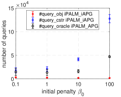
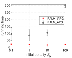
Fig. 1: Mean and standard deviation results by the proposed iPALM_iAPG and iPALM_APG with different values of initial penalty parameter $\beta_{0}$ on solving 10 random instances of the constrained LASSO problem (7.2) with $m=2000$ and $n=5000$.

7.3 Portfolio optimization

In this subsection, we test the proposed method iPALM_iAPG on solving the portfolio optimization:

(7.3) $$\min_{\mathbf{x}}\textstyle\frac{1}{2}{\mathbf{x}}^{\top}{\mathbf{Q}}{\mathbf{x}},\mbox{ s.t. }{\mathbf{x}}\geqslant\mathbf{0},\ \sum_{i=1}^{n}x_{i}\leqslant 1,\ {\boldsymbol{\xi}}^{\top}{\mathbf{x}}\geqslant c,\vspace{-0.1cm}$$

where ${\boldsymbol{\xi}}$ is the vector of expected return rate of $n$ assets, ${\mathbf{Q}}$ is the covariance matrix of the return rates, and $c$ is the imposed minimum total return. We solve instances of (7.3) with synthetic data and the real NASDAQ dataset that has been used in [49].

For synthetic data, we set $c=0.02$ and ${\mathbf{Q}}=\frac{{\mathbf{H}}{\mathbf{H}}^{\top}}{\|{\mathbf{H}}\|^{2}}+\mu{\mathbf{I}}$ with ${\mathbf{H}}\in\mathbb{R}^{n\times m}$ generated from the standard Gaussian distribution and $\mu\in\{0,10^{-3},0.1\}$, and the entries of ${\boldsymbol{\xi}}$ independently follow uniform distribution on $[-1,2]$. The dimensions of ${\mathbf{H}}$ were set to $n=2000$ and $m=1000$, and thus the objective of (7.3) with the generated data is $\mu$-strongly convex. For each value of $\mu$, we generated 10 independent instances. We compared to the APD method in [15] and the primal-dual sliding (PDS) method in [35]. The parameters of iPALM_iAPG and APD were set to the same values as in section 7.2, and the parameters of PDS were set by following [35, Theorem 2.2] with $R=1$. The results are reported in Table 3, where cmpl represents the amount of violation of complementarity condition in the KKT system, and all other quantities have the same meanings as those in Table 2. From the results, we see that the proposed method iPALM_iAPG can be significantly more efficient than APD and PDS in terms of the running time. APD with line search is less efficient than APD without line search in this test, while iPALM_iAPG performed similarly well with and without line search. PDS required significantly fewer queries to the objective but much more queries to the constraint functions. This is because the inner loop of PDS needs to run to a theoretically-determined maximum number of iterations rather than to a computationally-checkable stopping condition.

For the NASDAQ dataset, ${\boldsymbol{\xi}}$ is the mean of 30-day return rates. The original covariance matrix ${\mathbf{Q}}_{0}\in\mathbb{R}^{2730\times 2730}$ is rank-deficient, and in (7.3), we set ${\mathbf{Q}}={\mathbf{Q}}_{0}+\mu{\mathbf{I}}$ with $\mu\in\{0,10^{-3},0.1\}$. We also set $c=0.02$. These instances have worse condition numbers than the previous randomly generated ones. Hence, besides setting a stopping tolerance to $\varepsilon=10^{-6}$, we also set a maximum running time to one hour. We found that APD with line search did not work well for these instances, possibly because of the rounding error during the line search. Hence, we only reported the results of APD without line search by explicitly computing the smoothness constants and setting constant stepsizes. The results by all compared methods are shown in Table 4. Again, we see that the proposed method iPALM_iAPG was significantly more efficient than APD and PDS in terms of running time. For the hardest case that corresponds to $\mu=0$, APD and PDS both failed to reach the desired accuracy within one hour. Similar to the instances with synthetic data, PDS required much more queries to the constraint functions, though its queries to the objective was significantly fewer than the proposed method.

Table 3: Results by the proposed method iPALM_iAPG with and without line search, the accelerated primal-dual (APD) method in [15] with and without line search, and the primal-dual sliding (PDS) method in [35] on solving 10 instances of the portfolio optimization (7.3) with independently generated synthetic data. The numbers in the parentheses are the standard deviations.

	Method	#query_obj	#query_cstr	pres	dres	cmpl	time
$\mu=0$	iPALM_iAPG no line search	2709(28.8)	315480(19209.5)	0.0e+00	8.2e-7(1.2e-7)	0.0e+00	7.2
	iPALM_iAPG with line search	3172(68.2)	14984(403.7)	0.0e+00	8.2e-7(1.2e-7)	0.0e+00	3.2
	APD no line search	9229(772.6)		0.0e+00	8.2e-7(1.2e-7)	0.0e+00	7.0
	APD with line search	11736(1109.8)		0.0e+00	8.2e-7(1.2e-7)	0.0e+00	10.9
	PDS	1578(514.6)	18738280(12011557.5)	3.5e-19(1.1e-18)	8.1e-7(1.2e-7)	3.2e-27(1.0e-26)	278.7
$\mu=10^{-3}$	iPALM_iAPG no line search	1451(20.4)	183307(4012.1)	4.3e-8(8.9e-9)	6.8e-7(8.3e-8)	1.7e-15(6.8e-16)	4.3
	iPALM_iAPG with line search	1782(25.5)	50905(2211.4)	4.2e-8(8.8e-9)	7.0e-7(7.9e-8)	1.7e-15(6.7e-16)	2.6
	APD no line search	20931(1489.6)		3.4e-9(1.1e-9)	6.9e-7(7.9e-8)	1.6e-16(4.9e-17)	15.1
	APD with line search	26949(2055.4)		2.5e-9(9.1e-10)	6.9e-7(7.9e-8)	1.2e-16(4.0e-17)	24.1
	PDS	526(20.0)	5008697(786935.0)	1.7e-18(1.8e-18)	6.8e-7(8.0e-8)	1.7e-25(6.4e-26)	74.9
$\mu=0.1$	iPALM_iAPG no line search	243(1.9)	24951(497.0)	1.4e-7(1.3e-8)	6.4e-8(5.4e-9)	2.8e-13(2.6e-14)	1.2
	iPALM_iAPG with line search	262(1.0)	22420(703.6)	1.4e-7(1.3e-8)	6.9e-8(1.4e-9)	2.8e-13(2.6e-14)	1.2
	APD no line search	36869(2361.9)		5.8e-14(1.8e-14)	1.4e-7(1.3e-8)	1.1e-19(3.6e-20)	26.3
	APD with line search	59976(5195.3)		2.9e-14(1.2e-14)	1.4e-7(1.3e-8)	5.7e-20(2.4e-20)	53.3
	PDS	110(1.8)	2216395(309914.2)	6.9e-19(1.5e-18)	1.3e-7(1.5e-8)	4.1e-24(3.5e-24)	33.2

Table 4: Results by the proposed method iPALM_iAPG with and without line search, the accelerated primal-dual (APD) method in [15] without line search, and the primal-dual sliding (PDS) method in [35] on solving instances of the portfolio optimization (7.3) with NASDAQ data.

	Method	#query_obj	#query_cstr	pres	dres	cmpl	time
$\mu=0$	iPALM_iAPG no line search	112704	5530144	0.0e+00	4.2e-07	9.2e-19	350.6
	iPALM_iAPG with line search	37235	715328	0.0e+00	4.2e-07	0.0e+00	97.0
	APD no line search	1118808		0.0e+00	1.3e-06	2.2e-17	3603.8
	PDS	54058	176318909	3.5e-18	1.1e-06	1.5e-25	3604.0
$\mu=10^{-3}$	iPALM_iAPG no line search	21314	375994	0.0e+00	2.3e-07	7.0e-14	54.1
	iPALM_iAPG with line search	48643	117194	0.0e+00	2.3e-07	7.1e-14	108.4
	APD no line search	1119046		0.0e+00	8.5e-07	4.9e-18	3603.6
	PDS	6278	8927446	0.0e+00	2.2e-07	0.0e+00	195.5
$\mu=0.1$	iPALM_iAPG no line search	3206	32178	4.4e-09	6.2e-08	4.8e-13	10.8
	iPALM_iAPG with line search	6601	16451	5.2e-09	6.2e-08	5.6e-13	17.8
	APD no line search	1119360		0.0e+00	9.0e-08	2.6e-21	3603.6
	PDS	1404	29512311	0.0e+00	5.6e-08	0.0e+00	591.7

8 Conclusions

We have presented an inexact accelerated proximal gradient (iAPG) method for solving structured composite convex optimization, which have two smooth components with significantly different computational costs. When the more costly component has a significantly smaller smoothness constant than the less costly one, the proposed iAPG can significantly reduce the overall complexity than its exact counterpart, by querying the more costly component less frequently than the less costly one. Using the iAPG method as a subroutine, we proposed gradient-based methods for solving affine-constrained composite convex optimization and for solving bilinear saddle-point structured nonsmooth convex optimization. Our methods can have significantly lower overall complexity than existing methods when the coefficient matrix (in the affine constraint or in the bilinear term) permits matrix-vector multiplications with low cost.

References

• [1] Z. Allen-Zhu and E. Hazan. Optimal black-box reductions between optimization objectives. Advances in Neural Information Processing Systems, 29:1614–1622, 2016.
• [2] A. Beck and M. Teboulle. A fast iterative shrinkage-thresholding algorithm for linear inverse problems. SIAM journal on imaging sciences, 2(1):183–202, 2009.
• [3] A. Beck and M. Teboulle. Smoothing and first order methods: A unified framework. SIAM Journal on Optimization, 22(2):557–580, 2012.
• [4] R. I. Bot, E. R. Csetnek, and D.-K. Nguyen. Fast augmented lagrangian method in the convex regime with convergence guarantees for the iterates. arXiv preprint arXiv:2111.09370, 2021.
• [5] R. I. Boţ and D.-K. Nguyen. Improved convergence rates and trajectory convergence for primal-dual dynamical systems with vanishing damping. Journal of Differential Equations, 303:369–406, 2021.
• [6] K. Bredies and H. Sun. Accelerated douglas-rachford methods for the solution of convex-concave saddle-point problems. arXiv preprint arXiv:1604.06282, 2016.
• [7] A. Chambolle and T. Pock. A first-order primal-dual algorithm for convex problems with applications to imaging. Journal of mathematical imaging and vision, 40(1):120–145, 2011.
• [8] Y. Chen, G. Lan, and Y. Ouyang. Optimal primal-dual methods for a class of saddle point problems. SIAM Journal on Optimization, 24(4):1779–1814, 2014.
• [9] Y. Chen, G. Lan, and Y. Ouyang. Accelerated schemes for a class of variational inequalities. Mathematical Programming, 165(1):113–149, 2017.
• [10] D. Dvinskikh and A. Gasnikov. Decentralized and parallel primal and dual accelerated methods for stochastic convex programming problems. Journal of Inverse and Ill-posed Problems, 29(3):385–405, 2021.
• [11] T. Evgeniou, C. A. Micchelli, M. Pontil, and J. Shawe-Taylor. Learning multiple tasks with kernel methods. Journal of machine learning research, 6(4), 2005.
• [12] B. R. Gaines, J. Kim, and H. Zhou. Algorithms for fitting the constrained lasso. Journal of Computational and Graphical Statistics, 27(4):861–871, 2018.
• [13] E. Gorbunov, D. Dvinskikh, and A. Gasnikov. Optimal decentralized distributed algorithms for stochastic convex optimization. arXiv preprint arXiv:1911.07363, 2019.
• [14] X. Gu, F.-L. Chung, H. Ishibuchi, and S. Wang. Multitask coupled logistic regression and its fast implementation for large multitask datasets. IEEE transactions on cybernetics, 45(9):1953–1966, 2014.
• [15] E. Y. Hamedani and N. S. Aybat. A primal-dual algorithm with line search for general convex-concave saddle point problems. SIAM Journal on Optimization, 31(2):1299–1329, 2021.
• [16] B. He, S. Xu, and J. Yuan. Indefinite linearized augmented lagrangian method for convex programming with linear inequality constraints. arXiv preprint arXiv:2105.02425, 2021.
• [17] B. He and X. Yuan. On the acceleration of augmented lagrangian method for linearly constrained optimization. Optimization online, 3, 2010.
• [18] X. He, R. Hu, and Y.-P. Fang. Convergence rate analysis of fast primal-dual methods with scalings for linearly constrained convex optimization problems. arXiv preprint arXiv:2103.10118, 2021.
• [19] X. He, R. Hu, and Y. P. Fang. Convergence rates of inertial primal-dual dynamical methods for separable convex optimization problems. SIAM Journal on Control and Optimization, 59(5):3278–3301, 2021.
• [20] X. He, R. Hu, and Y.-P. Fang. Fast convergence of primal-dual dynamics and algorithms with time scaling for linear equality constrained convex optimization problems. arXiv preprint arXiv:2103.12931, 2021.
• [21] X. He, R. Hu, and Y.-P. Fang. Inertial primal-dual methods for linear equality constrained convex optimization problems. arXiv preprint arXiv:2103.12937, 2021.
• [22] X. He, R. Hu, and Y.-P. Fang. Perturbed primal-dual dynamics with damping and time scaling coefficients for affine constrained convex optimization problems. arXiv preprint arXiv:2106.13702, 2021.
• [23] Y. He and R. D. Monteiro. An accelerated hpe-type algorithm for a class of composite convex-concave saddle-point problems. SIAM Journal on Optimization, 26(1):29–56, 2016.
• [24] M. R. Hestenes. Multiplier and gradient methods. Journal of optimization theory and applications, 4(5):303–320, 1969.
• [25] B. Huang, S. Ma, and D. Goldfarb. Accelerated linearized bregman method. Journal of Scientific Computing, 54(2):428–453, 2013.
• [26] G. M. James, C. Paulson, and P. Rusmevichientong. Penalized and constrained optimization: an application to high-dimensional website advertising. Journal of the American Statistical Association, 2019.
• [27] K. Jiang, D. Sun, and K.-C. Toh. An inexact accelerated proximal gradient method for large scale linearly constrained convex sdp. SIAM Journal on Optimization, 22(3):1042–1064, 2012.
• [28] M. Kang, M. Kang, and M. Jung. Inexact accelerated augmented lagrangian methods. Computational Optimization and Applications, 62(2):373–404, 2015.
• [29] M. Kang, S. Yun, H. Woo, and M. Kang. Accelerated bregman method for linearly constrained $\backslash\ell_{1}-\backslash\ell_{2}$ minimization. Journal of Scientific Computing, 56(3):515–534, 2013.
• [30] G. Lan. Gradient sliding for composite optimization. Mathematical Programming, 159(1):201–235, 2016.
• [31] G. Lan, S. Lee, and Y. Zhou. Communication-efficient algorithms for decentralized and stochastic optimization. Mathematical Programming, 180(1):237–284, 2020.
• [32] G. Lan and R. D. Monteiro. Iteration-complexity of first-order penalty methods for convex programming. Mathematical Programming, 138(1):115–139, 2013.
• [33] G. Lan and R. D. Monteiro. Iteration-complexity of first-order augmented lagrangian methods for convex programming. Mathematical Programming, 155(1-2):511–547, 2016.
• [34] G. Lan and Y. Ouyang. Accelerated gradient sliding for structured convex optimization. arXiv preprint arXiv:1609.04905, 2016.
• [35] G. Lan, Y. Ouyang, and Y. Zhou. Graph topology invariant gradient and sampling complexity for decentralized and stochastic optimization. arXiv preprint arXiv:2101.00143, 2021.
• [36] G. Lan and Y. Zhou. Conditional gradient sliding for convex optimization. SIAM Journal on Optimization, 26(2):1379–1409, 2016.
• [37] H. Li, C. Fang, and Z. Lin. Convergence rates analysis of the quadratic penalty method and its applications to decentralized distributed optimization. arXiv preprint arXiv:1711.10802, 2017.
• [38] Z. Li and Y. Xu. Augmented lagrangian–based first-order methods for convex-constrained programs with weakly convex objective. INFORMS Journal on Optimization, 2021.
• [39] Q. Lin and L. Xiao. An adaptive accelerated proximal gradient method and its homotopy continuation for sparse optimization. Computational Optimization and Applications, 60(3):633–674, 2015.
• [40] A. Nemirovski. Prox-method with rate of convergence o (1/t) for variational inequalities with lipschitz continuous monotone operators and smooth convex-concave saddle point problems. SIAM Journal on Optimization, 15(1):229–251, 2004.
• [41] A. S. Nemirovskij and D. B. Yudin. Problem complexity and method efficiency in optimization. 1983.
• [42] Y. Nesterov. Introductory lectures on convex optimization: A basic course, volume 87. Springer Science & Business Media, 2003.
• [43] Y. Nesterov. Excessive gap technique in nonsmooth convex minimization. SIAM Journal on Optimization, 16(1):235–249, 2005.
• [44] Y. Nesterov. Smooth minimization of non-smooth functions. Mathematical programming, 103(1):127–152, 2005.
• [45] Y. Nesterov. Gradient methods for minimizing composite functions. Mathematical Programming, 140(1):125–161, 2013.
• [46] Y. Ouyang and T. Squires. Universal conditional gradient sliding for convex optimization. arXiv preprint arXiv:2103.11026, 2021.
• [47] Y. Ouyang and Y. Xu. Lower complexity bounds of first-order methods for convex-concave bilinear saddle-point problems. Mathematical Programming, 185(1):1–35, 2021.
• [48] A. Patrascu, I. Necoara, and Q. Tran-Dinh. Adaptive inexact fast augmented lagrangian methods for constrained convex optimization. Optimization Letters, 11(3):609–626, 2017.
• [49] Z. Peng, T. Wu, Y. Xu, M. Yan, and W. Yin. Coordinate-friendly structures, algorithms and applications. Annals of Mathematical Sciences and Applications, 1(1):57–119, 2016.
• [50] M. J. Powell. A fast algorithm for nonlinearly constrained optimization calculations. In Numerical analysis, pages 144–157. Springer, 1978.
• [51] R. T. Rockafellar. Augmented lagrangians and applications of the proximal point algorithm in convex programming. Mathematics of operations research, 1(2):97–116, 1976.
• [52] S. Sabach and M. Teboulle. Faster lagrangian-based methods in convex optimization. arXiv preprint arXiv:2010.14314, 2020.
• [53] M. Schmidt, N. L. Roux, and F. Bach. Convergence rates of inexact proximal-gradient methods for convex optimization. arXiv preprint arXiv:1109.2415, 2011.
• [54] M. Tao and X. Yuan. Accelerated uzawa methods for convex optimization. Mathematics of Computation, 86(306):1821–1845, 2017.
• [55] Q. Tran-Dinh and V. Cevher. Constrained convex minimization via model-based excessive gap. Advances in Neural Information Processing Systems, 27:721–729, 2014.
• [56] Q. Tran-Dinh and V. Cevher. A primal-dual algorithmic framework for constrained convex minimization. arXiv preprint arXiv:1406.5403, 2014.
• [57] Q. Tran-Dinh, O. Fercoq, and V. Cevher. A smooth primal-dual optimization framework for nonsmooth composite convex minimization. SIAM Journal on Optimization, 28(1):96–134, 2018.
• [58] P. Tseng. On accelerated proximal gradient methods for convex-concave optimization. submitted to SIAM Journal on Optimization, 2(3), 2008.
• [59] X. Wei, H. Yu, Q. Ling, and M. J. Neely. Solving non-smooth constrained programs with lower complexity than O (1/$\varepsilon$) a primal-dual homotopy smoothing approach. In Proceedings of the 32nd International Conference on Neural Information Processing Systems, pages 3999–4009, 2018.
• [60] Y. Xu. Accelerated first-order primal-dual proximal methods for linearly constrained composite convex programming. SIAM Journal on Optimization, 27(3):1459–1484, 2017.
• [61] Y. Xu. First-order methods for problems with ${O}(1)$ functional constraints can have almost the same convergence rate as for unconstrained problems. arXiv preprint arXiv:2010.02282, 2020.
• [62] Y. Xu. First-order methods for constrained convex programming based on linearized augmented lagrangian function. Informs Journal on Optimization, 3(1):89–117, 2021.
• [63] Y. Xu. Iteration complexity of inexact augmented lagrangian methods for constrained convex programming. Mathematical Programming, 185(1):199–244, 2021.
• [64] Y. Xu, I. Akrotirianakis, and A. Chakraborty. Proximal gradient method for huberized support vector machine. Pattern Analysis and Applications, 19(4):989–1005, 2016.
• [65] Y. Xu and W. Yin. A block coordinate descent method for regularized multiconvex optimization with applications to nonnegative tensor factorization and completion. SIAM Journal on Imaging Sciences, 6(3):1758–1789, 2013.
• [66] W. Yin. Analysis and generalizations of the linearized bregman method. SIAM Journal on Imaging Sciences, 3(4):856–877, 2010.
• [67] W. Yin, S. Osher, D. Goldfarb, and J. Darbon. Bregman iterative algorithms for $\backslash$ell_1-minimization with applications to compressed sensing. SIAM Journal on Imaging sciences, 1(1):143–168, 2008.
• [68] A. Yurtsever, Q. Tran-Dinh, and V. Cevher. A universal primal-dual convex optimization framework. In Proceedings of the 28th International Conference on Neural Information Processing Systems-Volume 2, pages 3150–3158, 2015.
• [69] R. Zhao. Accelerated stochastic algorithms for convex-concave saddle-point problems. arXiv preprint arXiv:1903.01687, 2019.
• [70] R. Zhao, W. B. Haskell, and V. Y. Tan. An optimal algorithm for stochastic three-composite optimization. In The 22nd International Conference on Artificial Intelligence and Statistics, pages 428–437. PMLR, 2019.