Gradient descent dynamics and the jamming transition in infinite dimensions

Abstract

Gradient descent dynamics in complex energy landscapes, i.e. featuring multiple minima, finds application in many different problems, from soft matter to machine learning. Here, we analyze one of the simplest examples, namely that of soft repulsive particles in the limit of infinite spatial dimension $d$. The gradient descent dynamics then displays a jamming transition: at low density, it reaches zero-energy states in which particles’ overlaps are fully eliminated, while at high density the energy remains finite and overlaps persist. At the transition, the dynamics becomes critical. In the $d\rightarrow\infty$ limit, a set of self-consistent dynamical equations can be derived via mean field theory. We analyze these equations and we present some partial progress towards their solution. We also study the Random Lorentz Gas in a range of $d=2\ldots 22$, and obtain a robust estimate for the jamming transition in $d\rightarrow\infty$. The jamming transition is analogous to the capacity transition in supervised learning, and in the appendix we discuss this analogy in the case of a simple one-layer fully-connected perceptron.

I Introduction

Gradient descent (GD) dynamics is one of the simplest dynamics one can imagine. It consists in following the gradient of an energy function in search of a local minimum. Yet, if the energy function is sufficiently complex, i.e. it features multiple minima and saddle points, GD dynamics can lead to an unexpectedly complex phenomenology. For example, in simple models for spin glasses, it features persistent aging dynamics, as first demonstrated in the pioneering work of Cugliandolo and Kurchan [1, 2, 3], and subsequently developed in, among others, Refs. [4, 5, 6, 7, 8, 9]: the energy decays to its asymptotic value as a power law, and the correlation functions continue to evolve at all times. The system keeps descending into the landscape, going through saddle points of lower and lower order, getting closer and closer to local minima but never reaching them [1, 7].

GD dynamics finds application in many contexts, especially related to theoretical computer science and optimization problems, i.e. when one needs to minimize a cost or loss function. A renowned example is given by machine learning, especially considering supervised learning. In this case, one has to learn an unknown function to relate an input data $x$ to an output label $y=f(x)$, based on a training set where the relation between the input data (e.g. the pixels of an image) and the output label (e.g. “cat” or “dog”) is known. The unknown function $f(x)$ is then parametrized by a guess function $g(x;\theta)$, whose parameters $\theta$ can be learnt by minimizing a loss function accounting for the error made in labelling data from the training set. Also in this case the GD dynamics can be surprisingly complex [10, 11, 12, 13, 14, 15, 16, 17].

A special class of such loss minimization problems is obtained whenever the loss function associated to a single data point is continuous and perfectly vanishing when the data point is correctly classified, and positive otherwise, e.g. the so-called squared hinge loss [18, 19, 20, 21, 22]. The question then becomes whether a choice of parameters $\theta$ exists, such that all data points in the training set are perfectly classified, leading to a zero loss. This question defines a satisfiability transition [23, 24, 25, 26, 27]: if such a configuration exists, then all the constraints are satisfied (SAT phase), whereas the existence of some violated constraints for all possible configurations defines the UNSAT phase. In the UNSAT case, one can then shift the problem to an optimization problem, i.e. finding a configuration that minimizes the number of unsatisfied constraints. The SAT/UNSAT transition becomes sharp in the thermodynamic limit $N\rightarrow\infty$, and search algorithms critically slow down when looking for solutions near the transition [26, 24, 25, 23, 28]. In neural networks, the transition corresponds to a capacity transition [29, 30, 31, 32]; in the SAT phase, the network is able to perfectly learn the input-output association $y=f(x)$ for all training examples, while in the UNSAT phase this relation is not correctly learned for some of the training examples. In a typical setting [29], $P=\alpha N$ random inputs with corresponding labels are given as training data to a neural network of $N$ units, and there is a critical value $\alpha_{c}$ above which the system is unable to perfectly learn all the training examples, i.e. the available information exceed the storage capacity of the network. GD dynamics and constraint satisfaction problems (CSP) also find application in many other contexts, e.g. in the study of complex ecological [33, 34, 35] and economical systems [36, 37, 38].

We will be particularly interested here in the application to soft matter problems, in which one can consider an idealized model of emulsions or soft athermal colloids, i.e. an assembly of finite-range interacting soft repulsive particles [39]. Such a system displays a sharp jamming transition [40, 41, 42, 43], which is fully analogous to the capacity or satisfiability transition introduced above [18, 19]. At low density, the GD dynamics converges exponentially to a floppy, zero-energy state in which particle overlaps are fully eliminated (unjammed phase, SAT) [44, 45]. At high density instead, the GD dynamics closely resembles that of mean field spin glasses [46, 47], i.e. it displays power-law relaxation to the final energy with persistent aging, while particle overlaps persist at long times, leading to a finite asymptotic energy (jammed phase, UNSAT). The jamming phase transition that separates the two regimes displays diverging length and time scales [40, 41, 42, 43]. The aim of this work is to investigate to some extent the dynamical mean field theory (DMFT) equations [1, 2, 3, 48, 49, 50, 51, 52, 53, 13, 17, 14, 54, 8, 9] that describe GD dynamics in mean-field complex systems, which display a jamming transition. We will focus in particular on the infinite-dimensional limit of soft repulsive particles [53], and we will thus use the jamming terminology in the main text.

Our results are the following. First of all, in section II, we present some analytical results on the long-time behavior of the DMFT equations for GD dynamics in the unjammed (SAT) phase, and we obtain simple analytical expressions for the response kernel and the response function in terms of the long-time limit of a single one-time quantity, namely the contact number. From these results we derive analytically the vibrational spectrum of the Hessian in the final unjammed state, which is of the Marcenko-Pastur form, as suggested numerically for infinite-dimensional particles in [55], see also [56] (the same result had been previously obtained in the perceptron model [57]). Our calculation, however, misses the isolated eigenvalue that is responsible for critical slowing down around jamming [58, 28, 44, 59, 45]. Moreover, our analysis of the DMFT equations does not provide the location of the jamming transition, because we are unable to evaluate the long-time limit of the contact number.

We thus turn in section III to the numerical study of a finite-dimensional model to get additional insight on the convergence to the DMFT limit when $d\rightarrow\infty$. It has been shown [60, 61] that the Random Lorentz Gas (RLG) is a very convenient model for this kind of investigation. In the present context, the RLG model consists in a single tracer that interacts via a soft repulsive interaction with a set of randomly drawn obstacles. Despite the striking difference between a many-body dynamics as in particle systems and a single-particle dynamics as in the RLG, it has been shown that these problems converge to the same DMFT equations in the $d\rightarrow\infty$ limit [60, 61]. The simplicity of the RLG allows one to investigate it numerically over a wide range of $d$. We then confirm that the dynamics converge to the DMFT limit, and obtain some additional insight on the range of validity of the analytical results. We also obtain an estimate of the location of the jamming transition in $d\rightarrow\infty$.

In the conclusion section IV, we briefly discuss the state-of-the-art of the analytical calculations of the asymptotic energy for GD dynamics in complex landscapes. We show that none of these methods is able to provide the correct asymptotic energy in the UNSAT phase, and we discuss some possible routes towards the solution of the problem.

In the appendix, in order to show the generality of the approach, we discuss the single-layer fully-connected perceptron [18, 19, 52, 57, 28], which is one of the simplest data classifiers in supervised machine learning. We show how the results of the main text can be translated to that case.

II Dynamical mean field theory

In this section, we recapitulate the DMFT equations for infinite-dimensional particle systems, as derived in [50, 51, 52, 53, 54]. We focus on the specific case of GD dynamics of soft repulsive spheres, see e.g. the discussion in [62, chapter 9]. Unfortunately, these equations are particularly difficult to solve numerically [63]. We discuss here some analytical results, while the numerical solution will be discussed in section III.

II.1 Definitions

For a system of $N$ particles with positions $\mathbf{x}_{i}(t)$ confined in a periodic volume $V\subset\mathbb{R}^{d}$, starting in equilibrium at infinite temperature $\beta_{0}=0$ (that corresponds to a uniformly random initial condition), consider the gradient descent equations:

$$\zeta\dot{\mathbf{x}}_{i}(t)=\bm{F}_{i}(t)\ ,\qquad\bm{F}_{i}(t)=-\frac{\partial V(\underline{X}(t))}{\partial\mathbf{x}_{i}(t)}\ ,\qquad V(\underline{X})=\sum_{i<j}v(\mathbf{x}_{i}-\mathbf{x}_{j})\ .$$ (1)

Important observables that characterize the dynamics are the correlation and response function

$${\cal C}(t,t^{\prime})=\frac{d}{\ell^{2}N}\sum_{i}\left\langle[\mathbf{x}_{i}(t)-\mathbf{x}_{i}(0)]\cdot[\mathbf{x}_{i}(t^{\prime})-\mathbf{x}_{i}(0)]\right\rangle\ ,\qquad{\cal R}(t,t^{\prime})=\frac{d}{\ell^{2}N}\sum_{i\mu}\frac{\delta\left\langle x_{i\mu}(t)\right\rangle}{\delta\lambda_{i\mu}(t^{\prime})}\ ,$$ (2)

where $\mu=1,\cdots,d$ is a coordinate index and ${\bm{\lambda}}_{i}(t)$ is an external field added to the force $\bm{F}_{i}(t)$ in order to compute the response, and the mean square displacement (MSD)

$$\Delta(t,t^{\prime})=\frac{d}{\ell^{2}N}\sum_{i}\left\langle[\mathbf{x}_{i}(t)-\mathbf{x}_{i}(t^{\prime})]^{2}\right\rangle\ ,\qquad\Delta_{r}(t)=\Delta(t,0)\ .$$ (3)

We take first the thermodynamic limit $N\rightarrow\infty$ and $V\rightarrow\infty$ at constant number density $\rho=N/V$. In [53] it is shown that if the limit $d\rightarrow\infty$ is taken next, with

• time $t$ remaining finite;

• potential $v(r)=\bar{v}(h)$, with $h=d(r/\ell-1)$ the scaled inter-particle gap and $\ell$ the particle diameter;

• packing fraction scaled as $\widehat{\varphi}=2^{d}\varphi/d$, with $2^{d}\varphi=\rho V_{d}\ell^{d}$ and $V_{d}$ the volume of a $d$-dimensional unit sphere;

• friction coefficient scaled as

  $$\widehat{\zeta}=\frac{\ell^{2}}{2d^{2}}\zeta\ ;$$ (4)

then the system dynamics is described by a set of one-dimensional stochastic equations with a Gaussian colored noise $\Xi(t)$, given by

$$\begin{split}&\widehat{\zeta}\dot{y}(t)=-\kappa(t)y(t)+\int_{0}^{t}\!\!\mathrm{d}t^{\prime}\,{\cal M}_{R}(t,t^{\prime})\,y(t^{\prime})-\bar{v}^{\prime}(h_{0}+y(t)+\Delta_{r}(t))+\Xi(t)\ ,\qquad y(0)=0\ ,\\ &\left\langle\Xi(t)\right\rangle=0\ ,\quad\left\langle\Xi(t)\Xi(t^{\prime})\right\rangle={\cal M}_{C}(t,t^{\prime})\ ,\\ \end{split}$$ (5)

with ${h(t)=h_{0}+y(t)+\Delta_{r}(t)}$ being the time-dependent inter-particle gap, and with memory kernels

$$\begin{split}\kappa(t)&=\frac{\widehat{\varphi}}{2}\int^{\infty}_{-\infty}\,\mathrm{d}h_{0}\,e^{h_{0}}\left\langle\bar{v}^{\prime\prime}(h(t))+\bar{v}^{\prime}(h(t))\right\rangle_{h_{0}}\ ,\\ {\cal M}_{C}(t,t^{\prime})&=\frac{\widehat{\varphi}}{2}\int^{\infty}_{-\infty}\mathrm{d}h_{0}\,e^{h_{0}}\langle\bar{v}^{\prime}(h(t))\bar{v}^{\prime}(h(t^{\prime}))\rangle_{h_{0}}\ ,\\ {\cal M}_{R}(t,t^{\prime})&=\frac{\widehat{\varphi}}{2}\int^{\infty}_{-\infty}\mathrm{d}h_{0}\,e^{h_{0}}\left.\frac{\delta\langle\bar{v}^{\prime}(h(t))\rangle_{h_{0},{\cal P}}}{\delta{\cal P}(t^{\prime})}\right|_{{\cal P}=0}=\frac{\widehat{\varphi}}{2}\int^{\infty}_{-\infty}\mathrm{d}h_{0}\,e^{h_{0}}\langle\bar{v}^{\prime\prime}(h(t))H(t,t^{\prime})\rangle_{h_{0}}\ .\end{split}$$ (6)

Here, the averages $\left\langle\bullet\right\rangle_{h_{0}}$ are over the noise $\Xi(t)$ at fixed $h_{0}=h(0)$, the perturbation ${{\cal P}(t)}$ acts via the replacement ${\bar{v}^{\prime}(h_{0}+y(t)+\Delta_{r}(t))\rightarrow\bar{v}^{\prime}(h_{0}+y(t)+\Delta_{r}(t)-{\cal P}(t))}$ in Eq. (5), and $H(t,t^{\prime})=\delta h(t)/\delta{\cal P}(t^{\prime})|_{{\cal P}=0}$, which, differentiating Eq. (5), satisfies

$$\widehat{\zeta}\frac{\partial}{\partial t}H(t,t^{\prime})=-\kappa(t)H(t,t^{\prime})-\bar{v}^{\prime\prime}(h(t))\left[H(t,t^{\prime})-\delta(t-t^{\prime})\right]+\int^{t}_{t^{\prime}}\mathrm{d}u\,{\cal M}_{R}(t,u)H(u,t^{\prime})\ .$$ (7)

Note that $H(t,t^{\prime})$ is a functional of $h(t)$, but we omit this dependence in order to simplify the notation. The correlation and response functions and the MSD are given by

$$\begin{split}\widehat{\zeta}\frac{\partial}{\partial t}{\cal C}(t,t^{\prime})=&-\kappa(t){\cal C}(t,t^{\prime})+\int_{0}^{t}\mathrm{d}u\,{\cal M}_{R}(t,u){\cal C}(u,t^{\prime})+\int_{0}^{t^{\prime}}\mathrm{d}u\,{\cal M}_{C}(t,u){\cal R}(t^{\prime},u)\ ,\\ \widehat{\zeta}\frac{\partial}{\partial t}{\cal R}(t,t^{\prime})=&\frac{\delta(t-t^{\prime})}{2}-\kappa(t){\cal R}(t,t^{\prime})+\int_{t^{\prime}}^{t}\mathrm{d}u\,{\cal M}_{R}(t,u){\cal R}(u,t^{\prime})\ ,\\ \frac{\widehat{\zeta}}{2}\frac{\partial}{\partial t}\Delta(t,t^{\prime})=&-\frac{\kappa(t)}{2}\left[\Delta(t,t^{\prime})+\Delta_{r}(t)-\Delta_{r}(t^{\prime})\right]+\frac{1}{2}\int_{0}^{t}\mathrm{d}u\,{\cal M}_{R}(t,u)\left[\Delta_{r}(t)-\Delta_{r}(t^{\prime})+\Delta(u,t^{\prime})-\Delta(u,t)\right]\\ &+\int_{0}^{\max(t,t^{\prime})}\mathrm{d}u\,{\cal M}_{C}(t,u)\left[{\cal R}(t,u)-{\cal R}(t^{\prime},u)\right]\ .\\ \end{split}$$ (8)

Here $\Delta(t,t^{\prime})={\cal C}(t,t)+{\cal C}(t^{\prime},t^{\prime})-2{\cal C}(t,t^{\prime})$ with ${\cal C}(t,0)={\cal C}(0,t)=0$, hence $\Delta_{r}(t)\equiv\Delta(t,0)={\cal C}(t,t)$.

It is convenient to define the integrated responses,

$$\chi(t,t^{\prime})=\int^{t}_{t^{\prime}}\mathrm{d}u\,{\cal R}(t,u)\ ,\qquad\widehat{\chi}(t,t^{\prime})=\kappa(t)-\int^{t}_{t^{\prime}}\mathrm{d}u\,{\cal M}_{R}(t,u)\ ,$$ (9)

and $\widehat{\chi}(t,t^{\prime})$ encodes the response kernels as

$$\kappa(t)=\widehat{\chi}(t,t)\ ,\qquad{\cal M}_{R}(t,t^{\prime})=\theta(t-t^{\prime})\,\partial_{t^{\prime}}\widehat{\chi}(t,t^{\prime})\ .$$ (10)

Eqs. (5), (6), (7) and (8) form a closed set that can be in principle solved numerically. Using the integrated response $\widehat{\chi}(t,t^{\prime})$ instead of ${\cal M}_{R}(t,t^{\prime})$, one can write them in an alternative form (appendix B):

$$\begin{split}\widehat{\zeta}\dot{y}(t)&=-\int_{0}^{t}\!\!\mathrm{d}t^{\prime}\,\widehat{\chi}(t,t^{\prime})\,\dot{y}(t^{\prime})-\bar{v}^{\prime}(h(t))+\Xi(t)\ ,\qquad y(0)=0\ ,\\ \left\langle\Xi(t)\right\rangle&=0\ ,\quad\left\langle\Xi(t)\Xi(t^{\prime})\right\rangle={\cal M}_{C}(t,t^{\prime})\ ,\\ h(t)&=h_{0}+y(t)+\Delta_{r}(t)\ ,\\ \widehat{\zeta}\frac{\partial}{\partial t}H(t,t^{\prime})&=-\frac{1}{\widehat{\zeta}}\bar{v}^{\prime\prime}(h(t^{\prime}))\widehat{\chi}(t,t^{\prime})-\int^{t}_{t^{\prime}}\mathrm{d}u\,\widehat{\chi}(t,u)\frac{\partial}{\partial u}H(u,t^{\prime})-\bar{v}^{\prime\prime}(h(t))\left[H(t,t^{\prime})-\delta(t-t^{\prime})\right]\ ,\\ \widehat{\zeta}\frac{\partial}{\partial t}{\cal C}(t,t^{\prime})&=-\int_{0}^{t}\mathrm{d}u\,\widehat{\chi}(t,u)\frac{\partial}{\partial u}{\cal C}(u,t^{\prime})+\int_{0}^{t^{\prime}}\mathrm{d}u\,{\cal M}_{C}(t,u){\cal R}(t^{\prime},u)\ ,\\ \widehat{\zeta}\frac{\partial}{\partial t}{\cal R}(t,t^{\prime})&=\frac{\delta(t-t^{\prime})}{2}-\frac{1}{2\widehat{\zeta}}\widehat{\chi}(t,t^{\prime})-\int_{t^{\prime}}^{t}\mathrm{d}u\,\widehat{\chi}(t,u)\frac{\partial}{\partial u}{\cal R}(u,t^{\prime})\ ,\\ \frac{\widehat{\zeta}}{2}\frac{\partial}{\partial t}\Delta(t,t^{\prime})&=-\frac{1}{2}\int_{0}^{t}\mathrm{d}u\,\widehat{\chi}(t,u)\frac{\partial}{\partial u}\left[\Delta(u,t^{\prime})-\Delta(u,t)\right]+\int_{0}^{\max(t,t^{\prime})}\mathrm{d}u\,{\cal M}_{C}(t,u)\left[{\cal R}(t,u)-{\cal R}(t^{\prime},u)\right]\ ,\\ \Delta_{r}(t)&=\Delta(t,0)\ ,\\ \widehat{\chi}(t,t^{\prime})&=\frac{\widehat{\varphi}}{2}\int^{\infty}_{-\infty}\,\mathrm{d}h_{0}\,e^{h_{0}}\left\langle\bar{v}^{\prime\prime}(h(t))\left[1-\int^{t}_{t^{\prime}}\mathrm{d}u\,H(t,u)\right]+\bar{v}^{\prime}(h(t))\right\rangle_{h_{0}}\ ,\\ {\cal M}_{C}(t,t^{\prime})&=\frac{\widehat{\varphi}}{2}\int^{\infty}_{-\infty}\mathrm{d}h_{0}\,e^{h_{0}}\left\langle\bar{v}^{\prime}(h(t))\bar{v}^{\prime}(h(t^{\prime}))\right\rangle_{h_{0}}\ ,\end{split}$$ (11)

having exploited the initial conditions $y(0)={\cal C}(0,t)=0$ and ${\cal R}(t^{+},t)=1/(2\widehat{\zeta})$, $H(t^{+},t)=\bar{v}^{\prime\prime}(h(t))/\widehat{\zeta}$. The time integrals are taken over $[t^{\prime}+\epsilon,t-\epsilon]$ for arbitrarily small $\epsilon$, excluding the singular contributions that have been accounted for separately.

We also recall the definition of the scaled energy, pressure and isostaticity index at infinite dimensions [53], which read, respectively,

$$\begin{split}e(t)&=\frac{\widehat{\varphi}}{2}\int^{\infty}_{-\infty}\,\mathrm{d}h_{0}\,e^{h_{0}}\left\langle\bar{v}(h(t)\right\rangle_{h_{0}}\ ,\\ p(t)&=-\frac{\widehat{\varphi}}{2}\int^{\infty}_{-\infty}\,\mathrm{d}h_{0}\,e^{h_{0}}\left\langle\bar{v}^{\prime}(h(t)\right\rangle_{h_{0}}\ ,\\ c(t)&=\frac{\widehat{\varphi}}{2}\int^{\infty}_{-\infty}\,\mathrm{d}h_{0}\,e^{h_{0}}\left\langle\theta(-h(t))\right\rangle_{h_{0}}\ ,\\ \end{split}$$ (12)

where the isostaticity index $c(t)=z(t)/(2d)$ is the number of contacts per particle $z(t)$ divided by the isostatic number $z=2d$, which is the minimal number of contacts required for mechanical stability [62].

II.2 Long-time limit of the dynamics in the unjammed phase

In the following we consider the harmonic soft sphere potential [39], which in infinite dimensions corresponds to $\bar{v}(h)=\varepsilon h^{2}\theta(-h)/2$ [62], and we fix $\varepsilon=1$ and $\widehat{\zeta}=1$ for simplicity, and without loss of generality.

For infinite-dimensional particle systems, the GD dynamics in the jammed phase is expected to display a non-trivial aging dynamics, belonging to the same universality class of $p$-spin models [1, 6, 7]. The energy should then decay as a power-law and correlation functions should age indefinitely; numerical evidence for this has been given in [46, 47]. It is not clear if the memory of the initial condition is lost or not [6, 7]: in finite dimensions, the MSD with respect to the initial condition, i.e. $\Delta_{r}(t)$, reaches a finite plateau, thus suggesting a persistent memory of the initial condition [47]. However, this pleateau seems to increase upon increasing $d$. Our numerical results (see section III) also suggest that, in the $d\rightarrow\infty$ limit, $\Delta_{r}(t)$ keeps growing with $t$, but they are not conclusive. Because the asymptotic dynamics in this regime is extremely difficult to describe [1, 6, 7, 8], we do not consider the jammed phase here; some speculations will be presented in the conclusion section IV.

We focus instead on the unjammed phase, where the gradient descent dynamics converges exponentially to a unique final configuration [28, 45], and we follow similar steps as in Ref. [14]. Because at long times motion is arrested, we have

$$\lim_{t\rightarrow\infty}\Delta(t+\tau,t)=\Delta^{\infty}(\tau)=0\ ,\qquad\forall\tau\ ,\qquad\text{and}\qquad\lim_{t\rightarrow\infty}\Delta_{r}(t)=\Delta_{r}^{\infty}\ ,$$ (13)

and a constant effective gap

$$\lim_{t\rightarrow\infty}h(t)=h_{\infty}=h_{0}+\Delta_{r}^{\infty}+y_{\infty}\geq 0\ ,$$ (14)

which is a positive random variable because by definition of the unjammed phase, all overlaps between particles are removed in the final state. Therefore

$$\begin{split}\kappa_{\infty}&=\lim_{t\rightarrow\infty}\kappa(t)=\frac{\widehat{\varphi}}{2}\int^{\infty}_{-\infty}\,\mathrm{d}h_{0}\,e^{h_{0}}\left\langle\bar{v}^{\prime\prime}(h_{\infty})+\bar{v}^{\prime}(h_{\infty})\right\rangle_{h_{0}}=\frac{\widehat{\varphi}}{2}\int^{\infty}_{-\infty}\,\mathrm{d}h_{0}\,e^{h_{0}}\left\langle\theta(-h_{\infty})\right\rangle_{h_{0}}=c_{\infty}\ ,\\ {\cal M}_{C}^{\infty}(\tau)&=\lim_{t\rightarrow\infty}{\cal M}_{C}(t+\tau,t)=\frac{\widehat{\varphi}}{2}\int^{\infty}_{-\infty}\mathrm{d}h_{0}\,e^{h_{0}}\langle\bar{v}^{\prime}(h_{\infty})^{2}\rangle_{h_{0}}=0\ ,\qquad\forall\tau\ .\end{split}$$ (15)

Following Ref. [14], we make an additional assumption, i.e. that the decay of the response kernel is fast enough to ensure that, for any function $f(t)$ that has a finite long-time limit, $f(t\rightarrow\infty)=f_{\infty}$,

$$\int_{0}^{t}\mathrm{d}u{\cal M}_{R}(t,u)f(u)\underset{t\rightarrow\infty}{\sim}\int_{0}^{t}\mathrm{d}u{\cal M}_{R}(t,u)f_{\infty}=[\kappa(t)-\widehat{\chi}(t,0)]f_{\infty}\ .$$ (16)

Under this assumption, the explicit time-dependence in Eq. (7) disappears when $t,t^{\prime}\rightarrow\infty$, and as a result response functions become time-translationally invariant (TTI):

$$\lim_{t\rightarrow\infty}H(t+\tau,t)=H^{\infty}(\tau)\qquad\Rightarrow\qquad\lim_{t\rightarrow\infty}{\cal M}_{R}(t+\tau,t)={\cal M}_{R}^{\infty}(\tau)\qquad\Rightarrow\qquad\lim_{t\rightarrow\infty}{\cal R}(t+\tau,t)={\cal R}^{\infty}(\tau)\ .$$ (17)

We also define the long-time limit of the integrated response kernels as

$$\chi=\lim_{t\rightarrow\infty}\chi(t,0)=\int_{0}^{\infty}\mathrm{d}\tau{\cal R}^{\infty}(\tau)\ ,\qquad\widehat{\chi}=\lim_{t\rightarrow\infty}\widehat{\chi}(t,0)=\kappa_{\infty}-\int_{0}^{\infty}\mathrm{d}\tau{\cal M}_{R}^{\infty}(\tau)\ .$$ (18)

Combining the previous results, the equation for $H^{\infty}(\tau)$ is

$$\partial_{\tau}H^{\infty}(\tau)=-[c_{\infty}+\theta(-h_{\infty})]H^{\infty}(\tau)+\theta(-h_{\infty})\delta(\tau)+\int_{0}^{\tau}\mathrm{d}u{\cal M}^{\infty}_{R}(\tau-u)H^{\infty}(u)\ .$$ (19)

Note that $h_{\infty}>0$ then implies $H^{\infty}(\tau)=0$ because the source term vanishes. Multiplying by $\bar{v}^{\prime\prime}(h_{\infty})=\theta(-h_{\infty})$ and averaging over $h_{0}$ as in Eq. (6), we obtain a closed equation for ${\cal M}^{\infty}_{R}(\tau)$:

$$\begin{split}\partial_{\tau}{\cal M}_{R}^{\infty}(\tau)&=-(c_{\infty}+1){\cal M}_{R}^{\infty}(\tau)+c_{\infty}\delta(\tau)+\int_{0}^{\tau}\mathrm{d}u{\cal M}^{\infty}_{R}(\tau-u){\cal M}_{R}^{\infty}(u)\ .\end{split}$$ (20)

In Laplace space, ${\cal M}_{R}^{\infty}(s)=\int_{0}^{\infty}\mathrm{d}\tau{\cal M}_{R}^{\infty}(\tau)e^{-s\tau}$, this gives

$$s{\cal M}^{\infty}_{R}(s)=-(1+c_{\infty}){\cal M}_{R}^{\infty}(s)+c_{\infty}+[{\cal M}^{\infty}_{R}(s)]^{2}\quad\Rightarrow\quad{\cal M}^{\infty}_{R}(s)=\frac{(1+c_{\infty}+s)-\sqrt{(1+c_{\infty}+s)^{2}-4c_{\infty}}}{2}\ .$$ (21)

Note that at short times we must have

$${\cal M}^{\infty}_{R}(\tau\rightarrow 0)\sim c_{\infty}+{\cal O}(t)\qquad\Leftrightarrow\qquad{\cal M}^{\infty}_{R}(s\rightarrow\infty)=\frac{c_{\infty}}{s}+{\cal O}(1/s^{2})\ ,$$ (22)

which fixes the choice of sign in Eq. (21), because the other solution has an unphysical behavior ${\cal M}^{\infty}_{R}(s)\sim s$ at large $s$. Note also that in order for Eq. (21) to be well defined we need the condition

$$(1+c_{\infty})^{2}\geq 4c_{\infty}\qquad\Leftrightarrow\qquad(1-c_{\infty})^{2}\geq 0\ ,$$ (23)

which is always satisfied. We also obtain

$$\widehat{\chi}=\kappa_{\infty}-{\cal M}^{\infty}_{R}(s=0)=\kappa_{\infty}-c_{\infty}=0\ ,$$ (24)

which guarantees a proper cancellation of the response kernels in the long time limit. Indeed, recalling that in the long time limit the noise vanishes and $h(t\rightarrow\infty)=h_{\infty}$, and applying Eq. (16) to the equation for $y(t)$ in Eq. (5), Eq. (24) implies:

$$0=-\kappa_{\infty}y_{\infty}+{\cal M}^{\infty}_{R}(s=0)y_{\infty}-\bar{v}^{\prime}(h_{\infty})=-\bar{v}^{\prime}(h_{\infty})\qquad\Rightarrow\qquad h_{\infty}\geq 0\ ,$$ (25)

which leaves $h_{\infty}$ indeterminate but ensures its positivity. Eq. (24) is therefore crucial for the consistency of the initial assumptions.

The Laplace transform in Eq. (21) can be inverted as

$${\cal M}^{\infty}_{R}(\tau)=\frac{\sqrt{c_{\infty}}}{\tau}e^{-(1+c_{\infty})\tau}I_{1}(2\sqrt{c_{\infty}}\tau)\ ,$$ (26)

where $I_{1}(x)$ is the modified Bessel function of first kind. Because $I_{1}(x)\sim e^{x}/\sqrt{2\pi x}$ at large $x$, we obtain that ${\cal M}^{\infty}_{R}(\tau)\sim e^{-(1-\sqrt{c_{\infty}})^{2}\tau}$ at large $\tau$, provided $c_{\infty}<1$, but when $c_{\infty}=1$ (the isostatic point) we obtain ${\cal M}^{\infty}_{R}(\tau)\sim\tau^{-3/2}$. Note that in both cases, the decay is fast enough to ensure the validity of Eq. (16).

Under the assumption of Eq. (15) we can inject the expression of ${\cal M}^{\infty}_{R}(\tau)$ in the equation for ${\cal R}(t,t^{\prime})$ and in Laplace space we get

$${\cal R}^{\infty}(s)=\frac{1}{2}\frac{1}{s+c_{\infty}-{\cal M}_{R}^{\infty}(s)}=\frac{1}{c_{\infty}-1+s+\sqrt{(1+c_{\infty}+s)^{2}-4c_{\infty}}}=\frac{1-c_{\infty}-s+\sqrt{(1+c_{\infty}+s)^{2}-4c_{\infty}}}{4s}\ ,$$ (27)

hence

$$\chi={\cal R}^{\infty}(s=0)=\infty\ ,$$ (28)

i.e. $\chi$ diverges in the whole unjammed phase, which indicates that the response function reaches a plateau at long times. When $s\rightarrow 0$ we have, from Eq. (27),

$${\cal R}^{\infty}(s)\sim\frac{1-c_{\infty}}{2s}\qquad\Rightarrow\qquad{\cal R}^{\infty}(\tau\rightarrow\infty)\rightarrow\frac{1-c_{\infty}}{2}\ .$$ (29)

II.3 Density of vibrational states

From the results of section II.2 we can derive the shape of the density of vibrational states in the unjammed phase, and get some physical insight on the origin of the TTI regime and of the plateau in the response function. At long times, the system reaches a unique configuration $\underline{X}^{*}=\{\mathbf{x}_{i}^{*}\}$. We can then linearize the dynamics around this configuration, with ${\bf y}_{i}(t)=\mathbf{x}_{i}(t)-\mathbf{x}_{i}^{*}$, and Eq. (1), with the inclusion of the external field $\bm{\lambda}_{i}(t)$, becomes

$$\zeta\dot{\bf y}_{i}(t)=-\sum_{j}\frac{\partial V(\underline{X}^{*})}{\partial\mathbf{x}_{i}\partial\mathbf{x}_{j}}\cdot{\bf y}_{j}(t)+\bm{\lambda}_{i}(t)=-\sum_{j}{\cal H}_{ij}\cdot{\bf y}_{j}(t)+\bm{\lambda}_{i}(t)\ ,$$ (30)

which is solved by

$$\underline{Y}(t)=\frac{1}{\zeta}\int_{0}^{t}\mathrm{d}u\,e^{-{\cal H}(t-u)/\zeta}\underline{\Lambda}(u)\ ,$$ (31)

where ${\cal H}$ is the Hessian in the minimum and $\underline{\Lambda}(t)=\{\bm{\lambda}_{i}(t)\}$ is the external field. The response function in this approximation can then be expressed in terms of the density of scaled vibrational states,

$$\rho(\lambda)=\frac{1}{Nd}\sum_{\alpha=1}^{Nd}\delta\left(\lambda-\frac{\ell^{2}\lambda_{\alpha}}{2\varepsilon d^{2}}\right)\ ,$$ (32)

as

$$\begin{split}{\cal R}^{\infty}(t)&=\left.\frac{d}{\ell^{2}N}\sum_{i\mu}\frac{\delta y_{i\mu}(t)}{\delta\lambda_{i\mu}(0)}\right|_{\bm{\lambda}=0}=\frac{d}{\ell^{2}\zeta N}\text{Tr}\,e^{-{\cal H}t/\zeta}=\frac{1}{2\widehat{\zeta}Nd}\text{Tr}\,e^{-{\cal H}t/\zeta}\\ &=\frac{1}{2\widehat{\zeta}Nd}\sum_{\alpha=1}^{Nd}e^{-\lambda_{\alpha}t/\zeta}=\frac{1}{2\widehat{\zeta}}\int\mathrm{d}\lambda\rho(\lambda)e^{-\varepsilon\lambda t/\widehat{\zeta}}\ ,\end{split}$$ (33)

which gives in Laplace space

$${\cal R}^{\infty}(s)=\frac{1}{2\varepsilon}\int\mathrm{d}\lambda\frac{\rho(\lambda)}{\lambda+\widehat{\zeta}s/\varepsilon}\ .$$ (34)

Note that the potential $V(\underline{X})$ has an energy scale $\varepsilon d^{2}$, hence the Hessian has a natural scale ${\cal H}\propto\varepsilon d^{2}/\ell^{2}$, which explains the scaling of $\lambda_{\alpha}$ in Eq. (32).

Combining Eqs. (34) and (27) (now with $\widehat{\zeta}=1$ and $\varepsilon=1$) we obtain the Cauchy transform (see e.g.  [64]) of $\rho(\lambda)$ in the form:

$$g(z)=\int\mathrm{d}\lambda\frac{\rho(\lambda)}{z-\lambda}=-2{\cal R}^{\infty}(s=-z)=\frac{1-c_{\infty}+z+\sqrt{(1+c_{\infty}-z)^{2}-4c_{\infty}}}{2z}\ ,$$ (35)

which shows that $\rho(\lambda)$ is the Marcenko-Pastur distribution with parameter $c_{\infty}<1$, i.e.

$$\rho(\lambda)=(1-c_{\infty})\delta(\lambda)+\frac{\sqrt{(\lambda_{+}-\lambda)(\lambda-\lambda_{-})}}{2\pi\lambda}\ ,\qquad\lambda_{\pm}=(1\pm\sqrt{c_{\infty}})^{2}\ .$$ (36)

This result provides a mathematical derivation of the conjecture proposed in Ref. [55]. The density of states displays a finite density of zero modes in the unjammed phase with $c_{\infty}<1$, which explains the finite plateau in the response function: if the system is perturbed away from the final state of the GD dynamics, it can be displaced along the zero modes, so that it never returns to the state it had before the perturbation. Finally, note that the present calculation gives the density of states in the thermodynamic limit, and it is thus unable to detect the isolated eigenvalue that is responsible for the critical slowing down upon approaching the jamming transition [58, 59, 45].

II.4 Dilute limit

Because the numerical solution of the DMFT equations is difficult, it is useful to consider here a low-density, dilute limit, to have an idea of what to expect at higher densities. In the very low-density limit, we can neglect all the kernels, because they have a factor $\widehat{\varphi}$ in front [63]. Following the same calculation line exposed in [65], the equations for correlation and response reduce to

$$\begin{split}\widehat{\zeta}\frac{\partial}{\partial t}{\cal R}(t,t^{\prime})&=\frac{\delta(t-t^{\prime})}{2}\quad\Rightarrow\quad{\cal R}(t,t^{\prime})=\frac{1}{2\widehat{\zeta}}\theta(t-t^{\prime})\ ,\\ \widehat{\zeta}\frac{\partial}{\partial t}{\cal C}(t,t^{\prime})&=0\quad\Rightarrow\quad{\cal C}(t,t^{\prime})=\Delta(t,t^{\prime})=0\ .\end{split}$$ (37)

The evolution equation for $h(t)$ then becomes

$$\widehat{\zeta}\dot{h}(t)=-\bar{v}^{\prime}(h(t))\quad\Rightarrow\quad h(t)=\begin{cases}h_{0}\,e^{-\varepsilon t/\widehat{\zeta}}&h_{0}<0\\ h_{0}&h_{0}\geq 0\end{cases}\ ,$$ (38)

and the fluctuating response $H(t,t^{\prime})$ then satisfies

$$\widehat{\zeta}\frac{\partial}{\partial t}H(t,t^{\prime})=-\bar{v}^{\prime\prime}(h(t))\left[H(t,t^{\prime})-\delta(t-t^{\prime})\right]\quad\Rightarrow\quad H(t,t^{\prime})=\frac{\varepsilon}{\widehat{\zeta}}\,e^{-\varepsilon(t-t^{\prime})/\widehat{\zeta}}\,\theta(t-t^{\prime})\,\theta(-h_{0})\ .$$ (39)

With these results we can compute the kernels. The instantaneous response is

$$\kappa(t)=\frac{\widehat{\varphi}}{2}\int^{0}_{-\infty}\mathrm{d}h_{0}\,e^{h_{0}}\,\varepsilon\,\left(1+h_{0}\,e^{-\varepsilon t/\widehat{\zeta}}\right)=\frac{\widehat{\varphi}}{2}\varepsilon\left(1-e^{-\varepsilon t/\widehat{\zeta}}\right)\ ,$$ (40)

the retarded response is

$${\cal M}_{R}(t,t^{\prime})=\frac{\widehat{\varphi}}{2}\int^{0}_{-\infty}\mathrm{d}h_{0}\,e^{h_{0}}\,\frac{\varepsilon^{2}}{\widehat{\zeta}}e^{-\varepsilon(t-t^{\prime})/\widehat{\zeta}}\,\theta(t-t^{\prime})=\frac{\widehat{\varphi}}{2}\frac{\varepsilon^{2}}{\widehat{\zeta}}\,e^{-\varepsilon(t-t^{\prime})/\widehat{\zeta}}\,\theta(t-t^{\prime})\ ,$$ (41)

and the integrated response is

$$\widehat{\chi}(t,0)=\int_{0}^{t}\mathrm{d}s\,{\cal M}_{R}(t,s)=\frac{\widehat{\varphi}}{2}\varepsilon\left(1-e^{-\varepsilon t/\widehat{\zeta}}\right)=\kappa(t)\ ,$$ (42)

which shows that $\widehat{\chi}(t,0)=\kappa(t)$ at all times in this limit. The noise correlation is

$${\cal M}_{C}(t,t^{\prime})=\frac{\widehat{\varphi}}{2}\int^{0}_{-\infty}\mathrm{d}h_{0}\,e^{h_{0}}\,\varepsilon^{2}\,h_{0}^{2}e^{-\varepsilon(t+t^{\prime})/\widehat{\zeta}}=\widehat{\varphi}\,\varepsilon^{2}\,e^{-\varepsilon(t+t^{\prime})/\widehat{\zeta}}\ .$$ (43)

Note that this correlation matrix is a projector, and as a consequence in the dilute limit the only randomness in the noise comes from its initial value, i.e. $\Xi(t)=\Xi(0)e^{-\varepsilon t/\widehat{\zeta}}$.

II.5 Methods for the numerical solution of the DMFT equations

The DMFT equations can be solved by means of two alternatives methods [66, 63, 67, 68, 69]:

• An iterative method, where we fix a maximum time $t_{\rm max}$ and we discretize the time with a step $\Delta t$, leading to a grid of $N_{t}=t_{\rm max}/\Delta t$ points. We then solve the self-consistent DMFT equations in the following way:

  1. Start with an initial guess for the memory kernels in Eq. (6). We typically set them to zero, as this corresponds to the dilute limit.

  2. Integrate the equations for the correlation and response functions in Eq. (8).

  3. Simulate the stochastic dynamics of Eqs. (5) to generate trajectories $y(t)$, and for each of them, integrate Eq. (7) to obtain $H(t,t^{\prime})$.

  4. Compute the new kernels in Eq. (6) averaging over the stochastic dynamics.

  5. Repeat until convergence.

  This scheme relies on the structure of the self-consistent equations for the memory kernels, which can be written as a kind of low-density expansion, i.e.

  $$\begin{split}\left\{\kappa_{i+1}(t),{\cal M}_{R,i+1}(t,t^{\prime}),{\cal M}_{C,i+1}(t,t^{\prime})\right\}&=\widehat{\varphi}\,{\cal F}[\left\{\kappa_{i}(t),{\cal M}_{R,i}(t,t^{\prime}),{\cal M}_{C,i}(t,t^{\prime})\right\}]\\ &\Downarrow\\ \kappa(t)&=\widehat{\varphi}\,\kappa^{(1)}(t)+\widehat{\varphi}^{2}\,\kappa^{(2)}(t)+\ldots\ ,\end{split}$$ (44)

  and so on for all the kernels, being $i$ the iteration step. The outcome of the first iteration is then given by the dilute solution at $\widehat{\varphi}\ll 1$ derived in section II.4, as we explicitly checked in the numerical implementation. This algorithm is the extension to the out-of-equilibrium case of the equilibrium algorithm implemented in [63].

• A step-by-step method, where we exploit the causal structure of the DMFT equations as follows. First of all, note that we only need to know the kernels for $t\geq t^{\prime}$, either because they are symmetric under exchange of times (correlation functions), or because they vanish for $t<t^{\prime}$ (response functions). Then, we can proceed as follows:

  1. Set the initial value of the kernels using their analytical expression in Eq. (6) at $t=t^{\prime}=0$.

  2. Integrate the first time step $\Delta t$ of the dynamical Eqs. (5), (7) and (8) with the memory kernels computed above; in particular we obtain a sample of values of $h(\Delta t)$.

  3. From these, we can numerically compute the kernels at $(t=\Delta t,t^{\prime}=0)$ and $(t=\Delta t,t^{\prime}=\Delta t)$ by averaging over the stochastic process.

  4. Repeat the procedure by extending at each step the stochastic trajectories $\{h(0),h(\Delta t),\ldots,h(t)\}$ to add a new point $h(t+\Delta t)$; from this, compute the kernels at subsequent times $t+\Delta t$ and $0\leq t^{\prime}\leq t+\Delta t$, given the kernels at previous times.

The two methods are theoretically equivalent and so are the expected outcomes. Using them, we could achieve the numerical integration of the DMFT equations for short trajectories of total duration $t\sim 10$ in natural units $\widehat{\zeta}=\varepsilon=1$. However, both methods become unreliable at long times because of a numerical instability in the generation of the correlated noise $\Xi(t)$ in Eq. (5). More precisely, the noise is generated in the following ways:

• Iterative algorithm: solving the eigenproblem for the correlation matrix $M_{ij}={\cal M}_{C}(i\Delta t,j\Delta t)$ at any iteration and generating the correlated noise $\Xi(t)$ independently before constructing each trajectory as

  $$\Xi(i\Delta t)\equiv\Xi_{i}=\sum_{j=0}^{N_{t}-1}\sqrt{\lambda_{j}}\,v_{i}^{j}\,\xi_{j}\ ,$$ (45)

  being $\lambda_{j}$ the $j$-th eigenvalue of the matrix $M$ and $v_{i}^{j}$ the $i$-th component of the corresponding eigenvector, and $\xi_{j}$ a Gaussian white noise of zero mean and covariance $\left\langle\xi_{i}\xi_{j}\right\rangle=\delta_{ij}$.

• Step-by-step algorithm: in this case the matrix $M$ is constructed step-by-step by extending existing trajectories, so we need to generate the noise $\Xi_{i}$ at time $t=i\Delta t$ for each trajectory, from the knowledge of the correlation matrix elements $M_{nm}$ at $n,m=0,\ldots,i$ and conditioned to the previous noise realization $(\Xi_{0},\ldots,\Xi_{i-1})$. This is done through the relation

  $$P(\Xi_{i}|\Xi_{0},\ldots,\Xi_{i-1})\propto\exp\left[-\frac{1}{2}\left(M^{-1}\right)_{ii}\Xi_{i}^{2}-\sum_{j=0}^{i-1}\left(M^{-1}\right)_{ij}\Xi_{j}\,\Xi_{i}\right]\ .$$ (46)

  Therefore $\Xi_{i}$ is Gaussian with mean $\left\langle\Xi_{i}\right\rangle=-\dfrac{1}{(M^{-1})_{ii}}\sum_{j=0}^{i-1}(M^{-1})_{ij}\Xi_{j}$ and variance $1/(M^{-1})_{ii}$.

The numerical instability in the noise generation is related to the physical behavior of the trajectories; when the GD dynamics approaches its final state, the force due to the self-consistent bath converges to a constant value, either vanishing (unjammed phase) or finite (jammed phase). In both cases, the correlation matrix develops almost-zero modes that lead to numerical instabilities either in the solution of the eigenproblem (iterative algorithm) or in the inversion of the correlation matrix (step-by-step algorithm). A second source of instability comes from the computation of memory kernels from Eq. (6): the trajectories flowing towards negative $h(t)$ starting from large positive $h_{0}$ have an exponential weight $e^{h_{0}}$ in the kernels, and are at the same time exponentially rare (as it should be to ensure convergence of the integration over $h_{0}$), thus leading to strong fluctuations in the numerical computation of the kernels. We were unfortunately not able to solve this problem. As a consequence of that, the numerical solution of the DMFT equations becomes unreliable at high density, and it is unable to describe the jamming transition properly, as we discuss in more details in sections III.

III Numerical results

We now compare the numerical solution of the DMFT equations discussed in section II with finite-dimensional numerical simulation results. For a study of the GD dynamics in many-body (MB) soft harmonic particle systems in varying $d$ we refer to Refs. [40, 41, 46, 44, 45, 47]. Because finite-dimensional MB systems converge quite slowly to the asymptotic $d\rightarrow\infty$ limit [70, 71, 72, 73], here we focus on the simpler Random Lorentz Gas (RLG) [60, 61], which is a single particle tracer with $d$ degrees of freedom embedded in a sea of random obstacles. In the limit $d\rightarrow\infty$, the MB problem can be mapped onto the RLG [60, 61], via a simple rescaling described in appendix C. In short, a given value of density $\widehat{\varphi}$ in the RLG corresponds to twice that value in the MB problem. At corresponding densities, one-time observables such as the energy and isostaticity index in Eq. (12) have equal values, the memory function of the MB problem is twice that of the RLG, and the MSD of the MB problem is half that of the RLG. Finally, the friction coefficient of the RLG has to be set as half that of the MB problem. All the results presented in this section will be expressed in RLG units, i.e. the DMFT results have been rescaled by appropriate factors as described above.

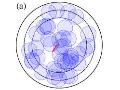
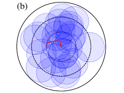
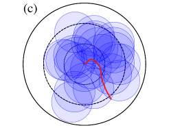
Figure 1: Illustration of three typical trajectories in the 2$d$ RLG, with $\widehat{\varphi}=1,A=7$ (a), $\widehat{\varphi}=3,A=2$ (b,c). In panels a (unjammed phase) and b (jammed phase), the tracer descends the energy landscape until it reaches a local minimum where it gets arrested, and the trajectory never escapes the 2$d$ sphere of radius $A/d$. In panel c, the tracer reaches the zero-energy endpoint in a region outside the cutoff radius, therefore leading to an unphysical trajectory for this problem. The obstacle radius is $\ell=1$, the dotted, dashed and full circle have radius $A/d$, $1+A/d$ and $2+A/d$ respectively.

III.1 Random Lorentz Gas

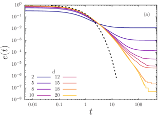
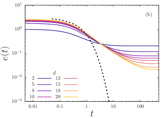
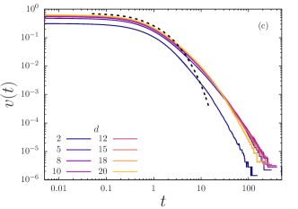
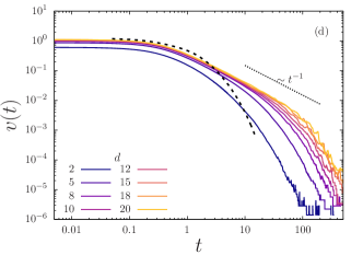
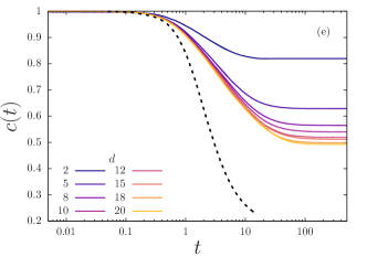
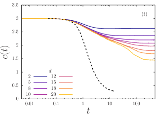
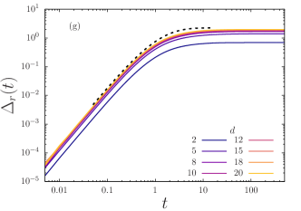
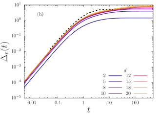
Figure 2: Time dependence of $e(t)$, $v(t)$, $c(t)$ and $\Delta_{r}(t)$ for the RLG, as obtained from the numerical solution of the DMFT equations in $d\rightarrow\infty$ (black dashed line: iterative method; the step-by-step method coincides at short times but becomes unreliable around $t\sim 1$) and from the direct numerical simulation at finite $d$ (colored lines). The finite-$d$ data converge to the DMFT predictions at short times, and converge upon increasing $d$ at all times, but the DMFT predictions are not reliable at long times, as also evidenced by the discrepancy between the two DMFT solution methods (not shown). At low density $\widehat{\varphi}=1$, the energy (a) and velocity (c) both decay exponentially, the isostaticity index (e) converges to a value $c_{\infty}<1$, and the MSD (g) goes to a finite plateau (unjammed phase). At large density $\widehat{\varphi}=3$, the energy (b) goes to a finite plateau, the velocity (d) decays as a power law over a range of times that increases with $d$, the long-time isostaticity index (f) is $c_{\infty}>1$, and the MSD (h) keeps increasing slowly with time when $d$ increases (jammed phase).

We simulate the dynamics of a point-like tracer moving in a $d$-dimensional space occupied by $N$ obstacles of radius $\ell$; the positions $\mathbf{X}_{i}$ ($i=1,\ldots,N$) of the latter are drawn independently and uniformly in space. Because of translational invariance, we can assume that the tracer starts at the origin without loss of generality. The microscopic dynamics of the tracer position $\mathbf{x}(t)$ then reads

$$\zeta\dot{\mathbf{x}}(t)=-\nabla V(\mathbf{x}(t))\ ,\qquad V(\mathbf{x})=\sum_{i=1}^{N}v(|\mathbf{x}-\mathbf{X}_{i}|)\ ,\qquad\mathbf{x}(0)=0\ .$$ (47)

This dynamics corresponds to the zero-noise limit of Ref. [61, Eq. (30)]. We analyze the case of a soft sphere interaction potential $v(r)=(d^{2}\varepsilon/2)(r/\ell-1)^{2}\theta(\ell-r)$, whose infinite-dimensional limit is equivalent to the potential $\bar{v}(h)=(\varepsilon/2)h^{2}\theta(-h)$ defined in section II. The friction coefficient must also be scaled with dimension through the relation $\zeta=(2d^{2}/\ell^{2})\widehat{\zeta}$, with $\widehat{\zeta}$ remaining finite in the infinite-dimensional limit. We fix $\varepsilon=1$, $\widehat{\zeta}=1/2$ (in such a way that the RLG value is half that of the MB problem, see appendix C) and $\ell=1$ without loss of generality, because these choices define a time and length unit. Under these assumptions, the dynamics read

$$\dot{\mathbf{x}}(t)=-\frac{1}{d}\sum^{N}_{i=1}\bar{v}^{\prime}(h_{i})\,\hat{\mathbf{r}}_{i}=-\frac{1}{d}\sum^{N}_{i=1}h_{i}\theta(-h_{i})\,\hat{\mathbf{r}}_{i}\ ,\qquad\hat{\mathbf{r}}_{i}=\dfrac{\mathbf{x}-\mathbf{X}_{i}}{|\mathbf{x}-\mathbf{X}_{i}|}\ ,\qquad h_{i}=d\left(\frac{|\mathbf{x}-\mathbf{X}_{i}|}{\ell}-1\right)\ .$$ (48)

The dynamics is therefore deterministic once the obstacles have been drawn. The number of obstacles represents the main computational challenge to the simulation. We draw obstacles in a spherical region of radius $R$, which then provides a cutoff on the maximal distance of an obstacle from the origin where the tracer starts its dynamics. This cutoff is justified if the displacement of the tracer’s trajectory from the origin never exceeds $R-\ell$, meaning that the tracer always explores a portion of space with a uniform obstacle density. The number of obstacles is then $N=\rho V=d\widehat{\varphi}(R/\ell)^{d}$, being $\rho=d\widehat{\varphi}/(V_{d}\ell^{d})$ and $V=V_{d}R^{d}$ the volume of the $d$-dimensional sphere of radius $R$. We therefore define $R=\ell(1+A/d)$, introducing the cutoff parameter $A$, so that at fixed $A$ the number of obstacles grows linearly rather than exponentially with $d$, namely $N\approx d\widehat{\varphi}e^{A}$. This choice will be justified a posteriori through the distribution of the tracer’s MSD.

The simulations are run by numerical integration of Eq. (48) using the Euler scheme with a fixed time step ${\Delta t=10^{-3}}$. The trajectories continue until the velocity becomes smaller than a threshold value, typically $|\dot{\mathbf{x}}(t)|<10^{-8}$, where we assume that a local minimum has been reached. Three examples of 2$d$ trajectories are shown in Fig. 1, illustrating the descent of the tracer in the obstacles’ energy landscape (both in the unjammed and jammed phases), and the escape from the cutoff radius in a high density trajectory. The dependence on the cutoff will be discussed in section III.3.

III.2 Time-dependent results

In Fig. 2 we plot the time evolution of the average (over the realizations of the obstacles) MSD $\Delta_{r}(t)=d\left\langle|\mathbf{x}(t)|^{2}\right\rangle$, energy $e(t)=\frac{1}{2d}\left\langle\sum_{i}h_{i}^{2}\theta(-h_{i})\right\rangle$, velocity $v(t)=\sqrt{-\dot{e}(t)}$ and isostaticity index $c(t)=\frac{1}{d}\left\langle\sum_{i}\theta(-h_{i})\right\rangle$, at two representative density values $\widehat{\varphi}=1.0$ and $3.0$, which are expected to be respectively below and above the jamming transition [62]. In all cases, we observe that at very short times, the two DMFT solution algorithms described in section II.5 coincide, and correctly describe the large-$d$ limit of the numerical data. Unfortunately, however, the agreement between the two DMFT solution schemes quickly worsen upon increasing time, and the DMFT numerical solution is thus not reliable at intermediate and long times. While we were unable to overcome this numerical limitation, we can still compare some exact asymptotic long-time predictions of DMFT with numerical data, see section III.4.

From the finite-$d$ simulation we can obtain insight on the behavior of the system (both MB, RLG and DMFT) in the $d\rightarrow\infty$ limit. Let us discuss first the case $\widehat{\varphi}=1$. We observe that the numerical data converge quite well upon increasing $d$, such that $d\approx 20$ with a cutoff $A\approx 7$ seems representative of the asymptotic limit. We observe that the energy and velocity both decay exponentially, and the isostaticity index converges to a value $c_{\infty}<1$. This is consistent with the expectation in the unjammed phase [44, 45]. Furthermore, the MSD goes to a finite plateau, indicating that the tracer relaxes over a few valleys before settling on the boundary of a final “lake” of zero energy, and that a lake can always be found at finite distance from any initial condition.

Conversely, for $\widehat{\varphi}=3$, the energy approaches a finite plateau at long times, while the velocity seems to decay as a power law, and the isostaticity index converges to a value $c_{\infty}>1$, consistently with the expectation for a jammed phase [46, 47]. In this case, while for any finite $d$ the MSD seems to converge to a finite plateau, the value of the plateau keeps increasing with dimension [47]. Furthermore, a slow time-dependence of the MSD seems to appear upon increasing $d$. This suggests the existence of persistent aging with weak ergodicity breaking (i.e. loss of the memory of the initial condition) [74] in the jammed phase [46, 47], akin to that of $p$-spin models [1, 7]. Because in the infinite-dimensional RLG the only non-trivial correlation is the MSD, weak ergodicity breaking implies that the MSD must keep growing at all times. Our data are, however, not conclusive on this issue, because the growth is modest and it is not clear whether it persists at longer times.

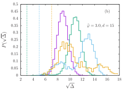
Figure 3: Probability distribution of the displacement $\sqrt{\Delta}=\sqrt{d}\,|\mathbf{x}_{\infty}|$ in the RLG at $\widehat{\varphi}=1$ (a) and $\widehat{\varphi}=3$ (b), $d=15$ and several values of $A$. At low densities the distributions converge upon increasing the cutoff when $A\geq 3.0$, while at high densities the distribution has not converged at $A=9.0$ and two peaks emerge. The vertical lines are placed at $x=A/\sqrt{d}$ with corresponding color codes. Panel c shows the average MSD versus $1/d$ for several values of $\widehat{\varphi}$ with $A=5$ (squares) and $A=7$ (circles). The points at $1/d=0$ are estimated from DMFT and the dashed lines are linear fits of the MSD at finite $d$.

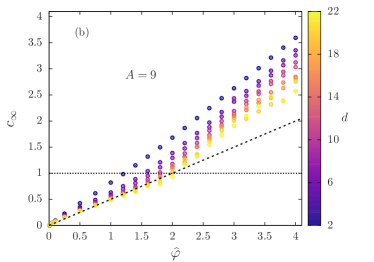
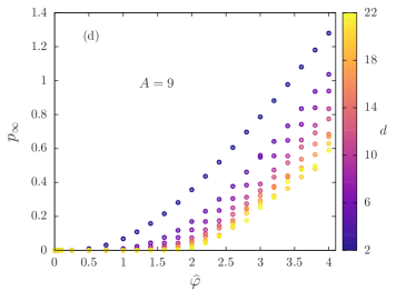
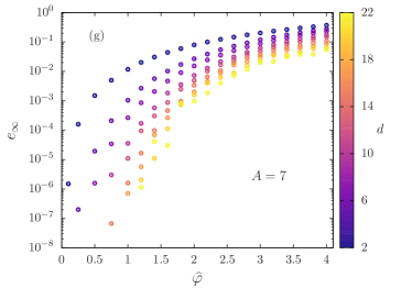
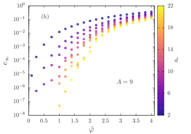
Figure 4: Average asymptotic values of the isostatiticy index $c_{\infty}=\lim_{t\rightarrow\infty}z(t)/d$, where $z(t)$ is the number of obstacles in contact with the RLG tracer at time $t$, of the pressure $p_{\infty}$, and of the energy $e_{\infty}$ (shown both in linear and log scales), as a function of density $\widehat{\varphi}$, for several values of $d$ and two values of $A=7$ (panels a, c, e, g) and $A=9$ (panels b, d, f, h). It is observed that $c_{\infty}\approx\widehat{\varphi}/2$, as predicted by the low-density expansion, up to the jamming transition point $\widehat{\varphi}=\widehat{\varphi}_{J}$ where $c_{\infty}=1$. Consistently, $p_{\infty}$ and $e_{\infty}$ are observed to vanish for $\widehat{\varphi}\lesssim\widehat{\varphi}_{J}$ upon increasing $d$, while $p_{\infty}$ grows linearly and $e_{\infty}$ grows quadratically in $\widehat{\varphi}-\widehat{\varphi}_{J}$ for $\widehat{\varphi}\gtrsim\widehat{\varphi}_{J}$.

III.3 Asymptotic long-time results and cutoff dependence

We now focus on the asymptotic results at long times. For each trajectory, we compute the final energy $e_{\infty}$, final pressure $p_{\infty}$, final isostatic index $c_{\infty}$, and final MSD $\Delta_{r}^{\infty}$. The cutoff dependence of the probability distribution of $\Delta_{r}^{\infty}$ over realizations of the disorder is shown in Fig. 3(a,b). At low densities and high dimensions, it converges with increasing $A$; conversely, at high density it becomes double-peaked upon increasing the cutoff and it does not converge within the accessible range of $A$. This is because the average value of $\Delta_{r}^{\infty}$ is larger (possibly divergent with $d\rightarrow\infty$, as discussed in section III.2) in this regime; at low $A$, the peak is due to the cutoff, i.e. all trajectories escape the sphere of radius $A/d$ and are thus unphysical, see Fig. 1(c). Upon increasing the cutoff, we start to observe a cutoff-independent “physical” peak, but the peak due to escaping trajectories remains visible, although it decreases with the cutoff. Clearly, the distribution would converge for larger $A$, but the number of obstacles then becomes exceedingly large for our available computational resources.

We also compare in Fig. 3(c) the rescaled MSD computed at $d=5,\ldots,22$ in the RLG with the prediction for $\Delta_{r}^{\infty}$ computed from the DMFT. At low densities, the MSD converges at $A\approx 5$ and a linear extrapolation at $d=\infty$ corresponds with the DMFT result. At higher densities the MSD does not converge with the cutoff nor with $d\rightarrow\infty$, and its value is also far from the DMFT prediction. This suggests once again that the DMFT numerical solution is not reliable, as discussed in section III.2.

Even if the available computational resources do not allow us to reach convergence in the cutoff at high density, we can still elucidate a somehow counterintuitive behavior of the dynamics, i.e. the increase of the MSD with density at fixed $d$. The situation is indeed inverted with respect to systems in thermal equilibrium, where a density increase yields the transition from diffusive to arrested dynamics and the asymptotic MSD decreases upon increasing density [63]; in this athermal case, in the low-density unjammed phase the tracer reaches the boundary of a zero-energy lake, and stops its motion there, leading to a finite displacement from the origin. Upon increasing the density, the tracer starts its dynamics from a higher energy level and it surfes over several energy valleys before reaching the zero-energy region. The final MSD from the origin thus increases with density. Whether the MSD diverges when jamming is reached remains an open problem. Under the weak ergodicity breaking scheme mentioned above [74, 1, 7], one should expect the MSD to diverge, because just above jamming, the tracer keeps surfing and surfing without ever finding a local minimum, so its MSD keeps increasing with time. While the data of Fig. 3(c) for the MSD seem to increase with $d$ when $\widehat{\varphi}\gtrsim\widehat{\varphi}_{J}$ and to saturate when $\widehat{\varphi}\lesssim\widehat{\varphi}_{J}$, they are, unfortunately, not conclusive, because our limited computational resources do not allow us to describe this regime in detail.

More precise information is obtained by plotting the asymptotic value of the average isostaticity index as a function of density, dimension, and cutoff, see Fig. 4. We observe that the data converge to a stable result when $A\approx 7$ and $d\approx 20$ in the regime $\widehat{\varphi}\lesssim 2.5$, in which $c_{\infty}\approx\widehat{\varphi}/2$ as predicted by the dilute limit of section II.4. As a consequence, we obtain $c_{\infty}\sim 1$ for $\widehat{\varphi}_{J}\approx 2$, which provides a rough estimate (to be refined below) of the jamming transition in the infinite-dimensional RLG, and therefore also suggests $\widehat{\varphi}_{J}\approx 4$ for the infinite-dimensional many-body problem, a value lower than that estimated in Ref. [62] by a less reliable procedure. The origin of this discrepancy is left for future investigation; in particular the simulations of the Mari-Kurchan model quoted in Ref. [62] should probably be extended to higher dimension. Consistently with this estimate, we observe that both $p_{\infty}$ and $e_{\infty}$ vanish upon increasing $d$ for $\widehat{\varphi}\lesssim 2$, suggesting that the tracer is reaching a zero-energy region without overlaps. On the contrary, for $\widehat{\varphi}\gtrsim 2$, we observe that $p_{\infty}$ grows linearly and $e_{\infty}$ grows quadratically in the distance from jamming, as observed in the MB problem [40, 41].

We obtain a more precise estimate of the jamming density $\widehat{\varphi}_{J}$ by extrapolating its value from the limit of $d,A\rightarrow\infty$. Therefore, we fit the pressure and energy functions as

$$\begin{split}p(\widehat{\varphi})&=ab\log\left(1+e^{(\widehat{\varphi}-\widehat{\varphi}_{J})/b}\right)\underset{b\approx 0^{+}}{\approx}a(\widehat{\varphi}-\widehat{\varphi}_{J})\theta(\widehat{\varphi}-\widehat{\varphi}_{J})\ ,\\ e(\widehat{\varphi})&=a\left[b\log\left(1+e^{(\widehat{\varphi}-\widehat{\varphi}_{J})/b}\right)\right]^{2}\underset{b\approx 0^{+}}{\approx}a(\widehat{\varphi}-\widehat{\varphi}_{J})^{2}\theta(\widehat{\varphi}-\widehat{\varphi}_{J})\ ,\end{split}$$ (49)

using $a$, $b$ and $\widehat{\varphi}_{J}$ as fitting parameters (distinct for the two observables).

We thus get a jamming point $\widehat{\varphi}_{J}(d,A)$ for every $d$ and $A$; keeping one of the two parameters constant, one can extrapolate an asymptotic value $\widehat{\varphi}_{J}(d)$ taking the intercept of a linear fit in $1/A$. Repeating the same extrapolation in $1/d$, one finally obtains the values for $\widehat{\varphi}_{J}=\lim_{d\rightarrow\infty}\lim_{A\rightarrow\infty}\widehat{\varphi}_{J}(d,A)$. The same procedure can be repeated by extrapolating first in $1/d$ and then $1/A$. Both are reported in Fig. 5. A conservative estimate of the jamming density therefore gives $\widehat{\varphi}_{J}=2.1\pm 0.2$.

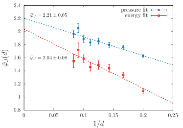
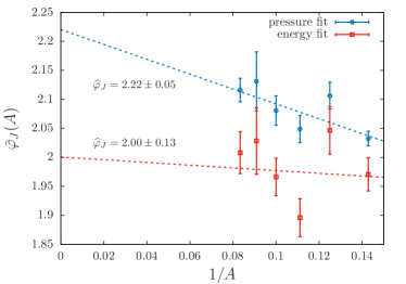
Figure 5: Jamming density $\widehat{\varphi}_{J}(d)$ vs. $1/d$ (left) or $\widehat{\varphi}(A)$ vs. $1/A$ (right). These values are obtained by first fitting the pressure and energy curves in Fig. 4 by means of Eq. (49), to obtain $\widehat{\varphi}_{J}(d,A)$, which is then fitted as $\widehat{\varphi}_{J}(d)+\alpha/A$ (left) or $\widehat{\varphi}_{J}(A)+\beta/d$ (right). The points represents the intercept of these extrapolations. Finally, the values $\widehat{\varphi}_{J}$ represent the intercepts of a second linear fit with respect to the other parameter. The final extrapolation is weakly dependent on the order of the two limits; conversely, the critical values obtained fitting the energy curves slightly differ from those obtained fitting the pressure curves.

III.4 Memory kernel and response function

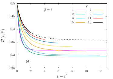
Figure 6: Plot of the $\hat{\chi}(t,t^{\prime})/\hat{\chi}(t^{\prime},t^{\prime})$ and ${\cal R}(t,t^{\prime})$ vs $t-t^{\prime}$ for various $t^{\prime}$ from DMFT (colored lines), to be compared with the stationary state predictions for $\hat{\chi}(\tau)/c^{\infty}$ and ${\cal R}^{\infty}(\tau)$ (black dashed lines).

Finally, we check the validity of the analytical computation of the long-time asymptotic memory kernel ${\cal M}^{\infty}_{R}(\tau)$ and response function ${\cal R}^{\infty}(\tau)$, given in Eqs. (26) and (27), respectively. We plot in Fig. 6(a,b) the integrated response kernel $\chi(t,t^{\prime})$ defined in Eq. (9), normalized by its value at equal times, as function of the time difference $t-t^{\prime}$. We compare the result obtained from the numerical solution of DMFT with the asymptotic prediction from Eq. (27), at the same rescaled densities discussed above, setting $c_{\infty}$ as the long-time limit of $c(t)$ obtained from the DMFT solution. The value of ${\cal R}^{\infty}(t)$ are obtained by the numerical inversion of the solution obtained in Laplace space. The curves in Fig. 6(c,d) show the convergence of the numerical solution to the TTI analytical solution in the unjammed phase, confirming the validity of the analysis of section II.2. Surprisingly, the analytical result matches the long-time behavior also in the jammed phase; this last feature may be a signal of a more robust validity of the theoretical prediction derived in Sec. II.2.

IV Conclusions and perspectives

In this paper, we have investigated the gradient descent dynamics of soft repulsive spheres in the limit $d\rightarrow\infty$, focusing in particular on the jamming dynamical transition.

In the unjammed phase, in which GD dynamics reaches zero energy, we have derived some analytical predictions for the long-time asymptotic dynamics, by analyzing the dynamical mean field theory equations. We have shown that the asymptotic solution of the DMFT equations can be written in closed form in terms of a single quantity, namely the asymptotic value $c_{\infty}$ of the contact number (section II.2). Most notably, we derived an expression for the response functions that implies a Marcenko-Pastur vibrational spectrum in the final state (section II.3), as conjectured in [55] (see also [57]). Unfortunately, the value of $c_{\infty}$ remains undetermined by the asymptotic analysis, and has to be derived from the full solution of the dynamics, as shown for example by the dilute limit (section II.4). The jamming transition point, which corresponds to $c_{\infty}=1$, thus remains undetermined. Another important problem that remains open is the derivation of the dynamical critical exponents that characterize the divergence of the relaxation time upon approaching the jamming transition from below [75, 76, 77, 45].

We then presented a (rather unsuccessful) attempt to solve numerically the DMFT equations. Unfortunately, our solution algorithms display convergence problems even at rather short times, thus preventing us to obtain reliable numerical predictions for the jamming transition from DMFT. Similar problems where encountered in Ref. [17]. To obtain more insight into the problem, we then simulated the Random Lorentz Gas in several dimensions ranging from $d=2$ to $d=22$. This study allowed us to confirm some predictions of DMFT, and more importantly to obtain an estimate of the jamming transition in $d\rightarrow\infty$, i.e. $\widehat{\varphi}_{J}\sim 2.1$ for the RLG and $\widehat{\varphi}_{J}\sim 4.2$ for the many-body problem. Note that this value is smaller than the dynamical Mode-Coupling transition, which is $\widehat{\varphi}_{\rm d}=4.8$ in $d\rightarrow\infty$ [62]. This result suggests that the so-called J-line [78, 79, 80, 81] extends to densities below the equilibrium glass transition in large enough dimensions, contrarily to what is found in physical dimensions $d=2,3$. This results confirms the idea that the equilibrium dynamical Mode-Coupling arrest is not relevant for the gradient descent dynamics [7], thus suggesting a very complex energy landscape in which zero-temperature jammed states can exist even in a region that is fully ergodic in presence of thermal noise [14].

The problem that remains strikingly open, in our opinion, is that of computing the asymptotic final energy $e_{\infty}$ reached by GD dynamics in the jammed (SAT) phase. We considered here the simplest case, in which GD starts from a fully random infinite-temperature initial condition, see [7] for the case where GD starts in equilibrium at finite temperature. Our numerical results for $e_{\infty}$ are reported in Fig. 4. Clearly, if one could compute this quantity analytically, one could then derive the jamming density at which $e_{\infty}=0$. Let us then review some approaches that have been proposed for the computation of $e_{\infty}$.

• First of all, one might wonder whether the system simply asymptotically reaches the ground state energy, i.e. $e_{\infty}=e_{\rm GS}$, which could then be computed by a standard thermodynamic zero-temperature calculation. However, such calculation can be done [82], and in the inifinite-dimensional limit [83] it predicts that the ground state energy is zero up to values of $\widehat{\varphi}$ that diverge when $d\rightarrow\infty$. Because our numerical results strongly suggest that $e_{\infty}$ remains finite for finite values of $\widehat{\varphi}\geq\widehat{\varphi}_{J}$ in the limit $d\rightarrow\infty$, this hypothesis can be ruled out, and the system must remain out of equilibrium in the asymptotic long-time limit.

• The first consistent out-of-equilibrium solution for the gradient descent dynamics in the long-time limit was obtained in the pioneering work of Cugliandolo and Kurchan [1]. Their asymptotic solution is based on the following assumptions: (i) memory of the initial condition is lost, i.e. $\Delta_{r}(t\rightarrow\infty)\rightarrow\infty$ in our formalism, which is deemed weak ergodicity breaking [74]; (ii) for large $t^{\prime}$ and $t>t^{\prime}$, there is a sharp separation between a short-time regime where the dynamics is time-translational invariant, $\Delta(t,t^{\prime})=\Delta(t-t^{\prime})$, and reaches equilibrium at temperature $T$ (here $T=0$ and $\Delta(t-t^{\prime})=0$) and a long-time regime where persistent aging is observed, with a scaling $\Delta(t,t^{\prime})=\overline{\Delta}[{\cal H}(t)/{\cal H}(t^{\prime})]$ with scaling functions $\overline{\Delta}[\lambda]$ and ${\cal H}(t)$; (iii) in the long-time regime correlations and responses are related by a modified effective temperature $T_{\rm eff}=T/m$; and (iv) dynamics is asymptotically marginal, i.e. the eigenvalue spectrum $\rho(\lambda)$ in the final state touches zero and as a consequence the response function and the energy have a power-law decay at long times (see section II.3). Based on these assumptions, Cugliandolo and Kurchan derived a consistent and exact asymptotic solution that also provides the value of $e_{\infty}$ in the spherical pure $p$-spin model [1]. It can be shown in full generality, see e.g.  [8] for a pedagogical derivation, that this asymptotic solution coincides with the zero-temperature version of the Monasson replica calculation [84], with the additional condition that the replicon eigenvalue vanishes [1, 4, 8]. Although the replica derivation is not needed, because the result can be fully derived from the DMFT equations [1, 8], it provides a simple recipe, and the corresponding formulae have been already derived in the literature [82, 83, 62]. In appendix D, we show that this asymptotic solution is inconsistent with our numerical data for the RLG, which suggests that some of its underlying assumptions are not verified in this system. This is also suggested by the fact that jammed packings display non-trivial critical exponents in their structural properties [40, 41, 42, 43, 85, 86] that are not captured by this asymptotic solution [80, 82, 62]. Hence, this solution can also be ruled out, at least in the vicinity of jamming.

• An attempt to go beyond this ansatz was presented by Montanari and Ricci-Tersenghi [87, 5] and then Rizzo [6]. Putting aside its dynamical justification, they extended the Monasson replica calculation mentioned above to take into account replica symmetry breaking. While, unfortunately, this scheme gives inconclusive results in what concerns the calculation of $e_{\infty}$ [87, 5, 6], it was shown in [88, 89] that it provides the correct critical exponents of jamming, see [62] for a detailed discussion. Yet, the value of $e_{\infty}$, and thus $\widehat{\varphi}_{J}$, still remain undetermined. An estimate of $\widehat{\varphi}_{J}$ within this approach (again, without a dynamical justification) was given in [88], but it overestimates our numerical results, and it moves from $\widehat{\varphi}_{J}=6.26$ ($\widehat{\varphi}_{J}=3.13$ in RLG units) to an even worse $\widehat{\varphi}_{J}=6.87$ ($\widehat{\varphi}_{J}=3.43$ in RLG units) upon increasing the steps of replica symmetry breaking. Hence, around the values of $\widehat{\varphi}_{J}$ we find numerically, no consistent solution of the full replica symmetry breaking equations in the Monasson scheme can be found. In summary, not only the dynamical meaning of this proposal remains obscure (except in the Cugliandolo-Kurchan scheme mentioned above), but it also cannot provide a consistent solution in the relevant regime of jamming densities. Yet, the fact that the jamming transition displayed by the asymptotic dynamics has the same critical properties of that obtained within this approach clearly calls for a first-principle justification, beyond the marginal stability argument put forward in [86]. Other replica approaches have been attempted, see [62] for a review, with similar drawbacks.

• Assumptions (ii) and (iii) in the Cugliandolo-Kurchan approach can be generalized to introduce a hierarchy of well separated time scales, each associated to an effective temperature [2, 3, 8, 9]. Such an approach provides a dynamical justification to full replica symmetry breaking, because it leads to the same set of equations. However, it is not clear to us how to fix the asymptotic dynamical energy within this approach, see [8] for a discussion.

• The other assumptions of the Cugliandolo-Kurchan solution should also be checked carefully. Results obtained on the Ising $p$-spin model seem to suggest that memory of the initial condition is not completely lost, even when the gradient descent dynamics is initialized in a fully random initial configurations [6], hence indicating strong ergodicity breaking. Similar results have been obtained for the Sherrington-Kirkpatrick model [90] and for spherical mixed $p$-spin models [91]. Our own results are inconclusive on this point. The validity of the weak ergodicity breaking is then not certain, at least in the vicinity of jamming. Concerning assumption (iv), it has also been suggested [6, 90] that the relaxation could be slower than a power-law (e.g. logarithmic). Our numerics is consistent with power-law relaxation, however, which suggests that marginality is a robust assumption.

Overall, we believe that despite much progress, the problem of investigating the long-time aging of GD dynamics, which was fully solved by Cugliandolo and Kurchan for the pure $p$-spin model [1], remains still open for more general models, including those investigated here. Our observations suggest that strong ergodicity breaking [6, 7, 90] and a multithermalization structure with an infinite hierarchy of time scales [2, 8, 9] should both be present in the proper asymptotic solution. Preliminary (and unsuccessful) attempts at constructing such kind of solutions have been presented in Refs. [4, 7]. Future work will hopefully provide better numerical algorithms to solve the DMFT equations, and thus provide insight on how to make further progress.

Data availability statement

The codes used to solve the DMFT equations and to simulate the RLG gradient descent are available at the GitHub repositories https://github.com/amanacorda/dmft_jamming.git and https://github.com/amanacorda/rlg_gd.git, respectively.

Appendix A The perceptron

In this appendix, we show how the results of section II can be adapted to the perceptron, the simplest supervised data classifier. We refer the reader to Refs. [19, 52] (and references therein) for an introduction to the model, and for recent work on its statics and dynamics.

A.1 Dynamical mean field equations for the perceptron model

We consider the harmonic perceptron Hamiltonian given by

$$H=\sum_{\mu=1}^{M}v(h_{\mu})\ ,\qquad h_{\mu}=\frac{1}{\sqrt{N}}\underline{\xi}^{\mu}\cdot\underline{x}-\sigma\ ,\qquad v(h)=\frac{1}{2}h^{2}\theta(-h)\ ,$$ (50)

and the gradient descent (GD) dynamics:

$$\dot{x}_{i}(t)=-\hat{\nu}(t)x_{i}(t)-\sum_{\mu}\frac{\xi^{\mu}_{i}}{\sqrt{N}}v^{\prime}(h_{\mu}(t))\ ,$$ (51)

where $\hat{\nu}(t)$ is a Lagrange multiplier needed to enforce the spherical constraint $|\underline{x}(t)|^{2}=N$, which can be expressed as

$$\hat{\nu}(t)=-\frac{1}{N}\sum_{\mu}(h_{\mu}(t)+\sigma)v^{\prime}(h_{\mu}(t))=-\alpha\left\langle(h(t)+\sigma)v^{\prime}(h(t))\right\rangle\ .$$ (52)

The DMFT equations corresponding to GD dynamics have been derived in Ref. [52], and are expressed in terms of an effective variable $h(t)$. If the initial condition is extracted at infinite temperature, i.e. uniformly on the sphere $|\underline{x}(t)|^{2}=N$, they read

$$\begin{split}\dot{h}(t)&=-\tilde{\nu}(t)[h(t)+\sigma]-v^{\prime}(h(t)-P(t))+\int_{0}^{t}\mathrm{d}sM_{R}(t,t^{\prime})[h(t^{\prime})+\sigma]+\eta(t)\ ,\qquad h(0)=h_{0}\ ,\\ P(h_{0})&=e^{-\frac{1}{2}(h_{0}+\sigma)^{2}}/\sqrt{2\pi}\ ,\\ M_{C}(t,t^{\prime})&=\langle\eta(t)\eta(t^{\prime})\rangle=\alpha\langle v^{\prime}(h(t))v^{\prime}(h(t^{\prime}))\rangle\ ,\\ M_{R}(t,t^{\prime})&=\left.\alpha\frac{\delta\langle v^{\prime}(h(t))\rangle}{\delta P(t^{\prime})}\right|_{P=0}\ ,\\ \tilde{\nu}(t)&=\hat{\nu}(t)+\alpha\langle v^{\prime\prime}(h(t))\rangle=\alpha\langle v^{\prime\prime}(h(t))-(h(t)+\sigma)v^{\prime}(h(t))\rangle=\int_{0}^{t}\mathrm{d}u\left[M_{R}(t,u)C(t,u)+M_{C}(t,u)R(t,u)\right]\ ,\\ \partial_{t}C(t,t^{\prime})&=-\tilde{\nu}(t)C(t,t^{\prime})+\int_{0}^{t}\mathrm{d}uM_{R}(t,u)C(u,t^{\prime})+\int_{0}^{t^{\prime}}\mathrm{d}uM_{C}(t,u)R(t^{\prime},u)\ ,\\ \partial_{t}R(t,t^{\prime})&=\delta(t-t^{\prime})-\tilde{\nu}(t)R(t,t^{\prime})+\int_{t^{\prime}}^{t}\mathrm{d}uM_{R}(t,u)R(u,t^{\prime})\ ,\end{split}$$ (53)

where the field $P(t)$ is only used to compute $M_{R}(t,t^{\prime})$ (with the derivative taken by keeping the kernels constant) and otherwise is set to $P=0$. Note that using the explicit expression for $\tilde{\nu}(t)$ in terms of an average over the process $h(t)$, the first five equations above provide closed equations for $h(t)$, $M_{C}(t,t^{\prime})$, $M_{R}(t,t^{\prime})$ and $\tilde{\nu}(t)$, without the need of solving for $C(t,t^{\prime})$ and $R(t,t^{\prime})$.

As in section II.1, it is convenient to derive an expression of the response function that does not require an explicit computation of the functional derivative. For this we write

$$M_{R}(t,t^{\prime})=\alpha\left\langle\frac{\delta v^{\prime}(h(t))}{\delta P(t^{\prime})}\right\rangle_{P=0}=\alpha\left\langle v^{\prime\prime}(h(t))\frac{\delta h(t)}{\delta P(t^{\prime})}_{P=0}\right\rangle=\alpha\left\langle v^{\prime\prime}(h(t))H(t,t^{\prime})\right\rangle_{P=0}\ ,\qquad H(t,t^{\prime})=\frac{\delta h(t)}{\delta P(t^{\prime})}_{P=0}\ .$$ (54)

Taking the functional derivative with respect to $P(t^{\prime})$ of the equation for $h(t)$, we obtain

$$\partial_{t}H(t,t^{\prime})=-\tilde{\nu}(t)H(t,t^{\prime})-v^{\prime\prime}(h(t))[H(t,t^{\prime})-\delta(t-t^{\prime})]+\int_{t^{\prime}}^{t}\mathrm{d}uM_{R}(t,u)H(u,t^{\prime})\ ,$$ (55)

with $H(t,t^{\prime})=0$ for $t<t^{\prime}$. This linear equation allows one to compute the function $H(t,t^{\prime})$ associated to each trajectory of $h(t)$. Note that another possible approach is to use the Novikov theorem [66], which gives

$$M_{R}(t,t^{\prime})=\int\mathrm{d}uM_{C}^{-1}(t^{\prime},u)\left\langle v^{\prime}(h(t))v^{\prime\prime}(h(t^{\prime}))\eta(u)\right\rangle\ ,$$ (56)

but this expression is not very practical for our purposes, because of the need to invert $M_{C}(t,t^{\prime})$ and of the presence of a three-point correlation.

As in section II.1, we define the integrated response:

$$\chi(t,t^{\prime})=\int_{t^{\prime}}^{t}\mathrm{d}uR(t,u)\ ,$$ (57)

and we note that an equation for $\chi(t,t^{\prime})$ can be obtained from the dynamical equation for $R(t,t^{\prime})$,

$$\dot{\chi}(t,t^{\prime})=1-\tilde{\nu}(t)\chi(t,t^{\prime})+\int_{0}^{t}\mathrm{d}uM_{R}(t,u)\chi(u,t^{\prime})\ .$$ (58)

We also define the integrated kernel of response, for $t>t^{\prime}$, as

$$\widehat{\chi}(t,t^{\prime})=\tilde{\nu}(t)-\int^{t}_{t^{\prime}}\mathrm{d}u\,M_{R}(t,u)\ ,$$ (59)

which encodes the kernels as

$$\tilde{\nu}(t)=\widehat{\chi}(t,t)\ ,\qquad M_{R}(t,t^{\prime})=\theta(t-t^{\prime})\,\partial_{t^{\prime}}\widehat{\chi}(t,t^{\prime})\ .$$ (60)

A.2 Some general properties of the long-time GD dynamics

We now discuss the general behavior of the GD dynamics in the long time limit.

A.2.1 Long-time TTI regime

Because the GD must converge to a unique final configuration, we must have

$$\lim_{t\rightarrow\infty}C(t+\tau,t)=C^{\infty}(\tau)=1\ ,\qquad\forall\tau\ .$$ (61)

At long times, the effective gap $h(t)$ must also converge to a constant value, $h_{\infty}$, which is itself a random variable, and therefore

$$\begin{split}\tilde{\nu}_{\infty}&=\lim_{t\rightarrow\infty}\tilde{\nu}(t)=\alpha\langle v^{\prime\prime}(h_{\infty})-(h_{\infty}+\sigma)v^{\prime}(h_{\infty})\rangle\ ,\\ M_{C}^{\infty}(\tau)&=\lim_{t\rightarrow\infty}M_{C}(t+\tau,t)=\alpha\langle v^{\prime}(h_{\infty})^{2}\rangle\ .\end{split}$$ (62)

Furthermore, in Eq. (55), when $t,t^{\prime}\rightarrow\infty$ we do not have any explicit time dependence, and as a result

$$\lim_{t\rightarrow\infty}H(t+\tau,t)=H^{\infty}(\tau)\qquad\Rightarrow\qquad\lim_{t\rightarrow\infty}M_{R}(t+\tau,t)=M_{R}^{\infty}(\tau)=\alpha\left\langle v^{\prime\prime}(h_{\infty})H^{\infty}(\tau)\right\rangle\ ,$$ (63)

with

$$\partial_{\tau}H^{\infty}(\tau)=-[\tilde{\nu}_{\infty}+v^{\prime\prime}(h_{\infty})]H^{\infty}(\tau)+v^{\prime\prime}(h_{\infty})\delta(\tau)+\int_{0}^{\tau}\mathrm{d}uM^{\infty}_{R}(\tau-u)H^{\infty}(u)\ .$$ (64)

Note that if $h_{\infty}>0$, then $v^{\prime\prime}(h_{\infty})=0$, which implies $H^{\infty}(\tau)=0$. Furthermore, from Eq. (59) we have

$$\widehat{\chi}^{\infty}(\tau)=\lim_{t\rightarrow\infty}\widehat{\chi}(t+\tau,t)=\tilde{\nu}_{\infty}-\int_{0}^{\tau}\mathrm{d}uM_{R}^{\infty}(u)\ ,\qquad\widehat{\chi}=\lim_{\tau\rightarrow\infty}\widehat{\chi}^{\infty}(\tau)=\tilde{\nu}_{\infty}-\int_{0}^{\infty}\mathrm{d}uM_{R}^{\infty}(u)\ .$$ (65)

Note that the response function also satisfies

$$\lim_{t\rightarrow\infty}R(t+\tau,t)=R^{\infty}(\tau)\ ,\qquad\partial_{t}R^{\infty}(\tau)=\delta(\tau)-\tilde{\nu}_{\infty}R(\tau)+\int_{0}^{\tau}\mathrm{d}uM^{\infty}_{R}(\tau-u)R^{\infty}(u)\ ,$$ (66)

and recalling Eq. (57) we can define

$$\chi=\lim_{\tau\rightarrow\infty}\lim_{t\rightarrow\infty}\chi(t+\tau,t)=\int_{0}^{\infty}\mathrm{d}uR^{\infty}(u)\ .$$ (67)

A.2.2 Exact solution for quadratic potential

Following section II.2, in the special case $v(h)=h^{2}\theta(-h)/2$ we have $v^{\prime\prime}(h)=\theta(-h)$ and we can thus obtain a closed equation for $M^{\infty}_{R}(\tau)$. Recalling Eq. (63), multiplying Eq. (64) by $v^{\prime\prime}(h_{\infty})$ and taking the average, we obtain

$$\begin{split}\partial_{\tau}M_{R}^{\infty}(\tau)&=-(1+\tilde{\nu}_{\infty})M_{R}^{\infty}(\tau)+c_{\infty}\delta(\tau)+\int_{0}^{\tau}\mathrm{d}uM^{\infty}_{R}(\tau-u)M_{R}^{\infty}(u)\ ,\qquad c_{\infty}=\alpha\left\langle\theta(-h_{\infty})\right\rangle\ ,\end{split}$$ (68)

where $c_{\infty}$ is the isostaticity index for the perceptron [19]. In Laplace space, this gives

$$sM^{\infty}_{R}(s)=-(1+\tilde{\nu}_{\infty})M_{R}^{\infty}(s)+c_{\infty}+[M^{\infty}_{R}(s)]^{2}\qquad\Rightarrow\qquad M^{\infty}_{R}(s)=\frac{(1+\tilde{\nu}_{\infty}+s)-\sqrt{(1+\tilde{\nu}_{\infty}+s)^{2}-4c_{\infty}}}{2}\ .$$ (69)

Note that at short times we must have

$$M^{\infty}_{R}(\tau\rightarrow 0)\sim c_{\infty}+{\cal O}(t)\qquad\Leftrightarrow\qquad M^{\infty}_{R}(s\rightarrow\infty)=\frac{c_{\infty}}{s}+{\cal O}(1/s^{2})\ ,$$ (70)

which fixes the choice of sign in Eq. (69), because the other solution has an unphysical behavior $M^{\infty}_{R}(s)\sim s$ at large $s$. Note also that in order for Eq. (69) to be well defined we need the condition

$$(1+\tilde{\nu}_{\infty})^{2}\geq 4c_{\infty}\ ,$$ (71)

whose meaning will be discussed below. The Laplace transform can be inverted and we get

$$M^{\infty}_{R}(\tau)=\frac{\sqrt{c_{\infty}}}{\tau}e^{-(1+\tilde{\nu}_{\infty})\tau}I_{1}(2\sqrt{c_{\infty}}\tau)\ ,$$ (72)

where $I_{1}(x)$ is the modified Bessel function of first kind. Injecting the expression of $M^{\infty}_{R}(\tau)$ in Eq. (66) in Laplace space, we get

$$R^{\infty}(s)=\frac{1}{s+\tilde{\nu}_{\infty}-M_{R}^{\infty}(s)}=\frac{2}{(\tilde{\nu}_{\infty}+s-1)+\sqrt{(1+\tilde{\nu}_{\infty}+s)^{2}-4c_{\infty}}}\ ,$$ (73)

hence

$$\chi=R^{\infty}(s=0)=\frac{2}{(\tilde{\nu}_{\infty}-1)+\sqrt{(1+\tilde{\nu}_{\infty})^{2}-4c_{\infty}}}\ .$$ (74)

A.3 Memory-less solution

We are now going make a stronger assumption as in Eq. (16), i.e. we assume that the convergence to the TTI regime described in appendix A.2.1 is fast enough, and the memory kernels decay fast enough, such that, for a function $f(t)$ that tends to a constant, $f(t\rightarrow\infty)=f_{\infty}$, one can write

$$\lim_{t\rightarrow\infty}\int_{0}^{t}\mathrm{d}t^{\prime}M_{R}(t,t^{\prime})f(t^{\prime})=\int_{0}^{\infty}\mathrm{d}\tau M_{R}^{\infty}(\tau)f_{\infty}=(\tilde{\nu}_{\infty}-\widehat{\chi})f_{\infty}\ ,$$ (75)

where we used Eq. (65). In other words, all the previous dynamical history is lost and only the TTI regime contributes at long times.

Because we know that the effective gap satisfies $h(t\rightarrow\infty)=h_{\infty}$, applying this assumption to the equation for $h(t)$ in Eq. (53), we obtain

$$0=-\widehat{\chi}(h_{\infty}+\sigma)-v^{\prime}(h_{\infty})+\eta_{\infty}\ ,\qquad\text{where}\qquad\langle\eta_{\infty}^{2}\rangle=\alpha\langle v^{\prime}(h_{\infty})^{2}\rangle=M_{C}^{\infty}\ .$$ (76)

Applying the same assumption to the equation for $\tilde{\nu}(t)$ in Eq. (53) we obtain

$$\widehat{\chi}=M_{C}^{\infty}\chi\ .$$ (77)

At this point, it is worth to note that $\chi$, which is the integral of the response function, can be finite or formally infinite. We analyze the two cases separately below.

A.3.1 UNSAT phase

The content of this appendix was communicated to us by P.Urbani at the beginning of this project, and is reported here for completeness; it has been published in Ref. [14] in a slightly different model. Let us suppose that $\chi$ is finite. This corresponds to a response function $R(t,t^{\prime})$ that decays sufficiently fast to be integrable. In other words, the final state reached by GD is such that, if the system is infinitesimally displaced away from it, it returns to the same state fast enough that the perturbation is integrable in time. Physically, this suggest that GD reaches a minimum that admits a harmonic expansion with well-defined and strictly positive frequencies; we come back to this point below. Using Eq. (77), Eq. (76) becomes

$$0=-M_{C}^{\infty}\chi(h_{\infty}+\sigma)-v^{\prime}(h_{\infty})+\eta_{\infty}\ .$$ (78)

We then need to eliminate $M_{C}^{\infty}$. Under the assumption that the GD converges sufficiently fast, and that the response function $R(t,t^{\prime})$ is integrable, we have $\lim_{t\rightarrow\infty}\chi(t,0)=\lim_{t\rightarrow\infty}\chi(t,t^{\prime})$ for all $t^{\prime}$, because the memory of the initial time is lost. By taking the limit $t\rightarrow\infty$ of Eq. (58), we then obtain

$$\widehat{\chi}=\frac{1}{\chi}\qquad\Rightarrow\qquad M_{C}^{\infty}=\chi^{-2}\ ,$$ (79)

which leads to a closed equation for $\chi$ by noting that

$$\eta_{\infty}=(h_{\infty}+\sigma)/\chi+v^{\prime}(h_{\infty})\ ,\qquad\langle\eta_{\infty}^{2}\rangle=\chi^{-2}=\alpha\langle v^{\prime}(h_{\infty})^{2}\rangle\ .$$ (80)

More explicitly, we have

$$P(h_{\infty})=P(\eta_{\infty})\frac{\mathrm{d}\eta_{\infty}}{\mathrm{d}h_{\infty}}=\frac{e^{-\frac{1}{2}\left(h_{\infty}+\sigma+\chi v^{\prime}(h_{\infty})\right)^{2}}}{\sqrt{2\pi}}\left(1+\chi v^{\prime\prime}(h_{\infty})\right)\ ,\qquad\chi^{-2}=\alpha\int\mathrm{d}h_{\infty}P(h_{\infty})v^{\prime}(h_{\infty})^{2}\ ,$$ (81)

which is a closed equation for $\chi$ from which all the other quantities can be derived. Specializing to $v(h)=h^{2}\theta(-h)/2$, we get

$$\frac{1}{\chi^{2}}=\frac{\alpha}{(1+\chi)^{2}}\int_{-\infty}^{0}\mathrm{d}hh^{2}\gamma_{1}(h+\sigma)\ ,$$ (82)

which is the same equation one gets from replicas [19] in the replica symmetric UNSAT phase of the perceptron. In fact, Eq. (81) gives a finite probability to negative gaps, $h_{\infty}<0$, which indicates that the system is in an UNSAT phase. Furthermore, the equation for $C(t,0)$ in the limit $t\rightarrow\infty$ gives

$$0=\widehat{\chi}C(\infty,0)\qquad\Rightarrow\qquad C(\infty,0)=0\ ,$$ (83)

which indicates a complete loss of correlation with the initial condition. This indicates that the ground state is unique, which is consistent with the replica symmetric ansatz and also with our initial assumption, that the response function at long times is integrable.

Given the expression of $P(h_{\infty})$, one can easily derive the expressions of $\tilde{\nu}_{\infty}$ and $c_{\infty}$, see Ref. [19]. Inserting these expressions into the exact result in Eq. (72), one can show that:

• $M^{\infty}_{R}(\tau)$ decays exponentially for $\sigma>0$ and all values of $\alpha>\alpha_{J}(\sigma)$ such that the system is in the UNSAT phase [19].

• When $\sigma=0$ and $\alpha>2$, one has $M^{\infty}_{R}(\tau)\sim\tau^{-3/2}$. This is the critical line on which replica symmetry is marginally broken [19].

• For $\sigma<0$ one obtains an inconsistency. In fact, the value of $\widehat{\chi}$ obtained from Eq. (77) corresponds to the wrong choice of sign in Eq. (69). This indicates that the assumption of loss of memory is incorrect in this case, and we know indeed that the system displays replica symmetry breaking and a complex landscape with multiple minima in the UNSAT phase for $\sigma<0$ [19].

A.3.2 SAT phase

Upon approaching the SAT phase, it is known from the replica analysis that $\chi\rightarrow\infty$ [19]. Indeed, this is the only way to suppress negative values of $h_{\infty}$, corresponding to unsatisfied gaps, in Eq. (81). We then expect that in the SAT phase one formally has $\chi=\infty$ and $M_{C}^{\infty}=0$, but with $\chi M_{C}^{\infty}=0$, as suggested by Eq. (79). This is also consistent with the observation that in the SAT phase, because $h_{\infty}\geq 0$ and $v^{\prime}(h_{\infty})=0$, one has $\tilde{\nu}_{\infty}=c_{\infty}$, see Eq. (62), which, once inserted into Eq. (73), gives for the response function

$$R^{\infty}(s)=\frac{2}{c_{\infty}-1+s+\sqrt{(1+c_{\infty}+s)^{2}-4c_{\infty}}}=\frac{1-c_{\infty}-s+\sqrt{(1+c_{\infty}+s)^{2}-4c_{\infty}}}{2s}\ ,$$ (84)

hence

$$\chi=R^{\infty}(s=0)=\infty\ ,$$ (85)

i.e. $\chi$ diverges in the whole unjammed phase, which indicates that the response function reaches a plateau at long times. When $s\rightarrow 0$ we have indeed

$$R^{\infty}(s)\sim\frac{1-c_{\infty}}{s}\qquad\Rightarrow\qquad R^{\infty}(\tau\rightarrow\infty)\rightarrow 1-c_{\infty}\ .$$ (86)

Physically, this corresponds to the fact that in the SAT phase the GD dynamics stops on the boundary of the finite volume of phase space corresponding to solutions, i.e. zero energy states. A random perturbation applied to this state has a finite probability to bring the system inside this volume, and as a consequence the system will not relax back to its initial state; the response function does not decay at long times and $\chi$ thus diverges.

Furthermore, setting $\tilde{\nu}_{\infty}=c_{\infty}$ in Eq. (72) and using $I_{1}(x)\sim e^{x}/\sqrt{2\pi x}$ at large $x$, we obtain that ${\cal M}^{\infty}_{R}(\tau)\sim e^{-(1-\sqrt{c_{\infty}})^{2}\tau}$ at large $\tau$, provided $c_{\infty}<1$, but when $c_{\infty}=1$ (the isostatic point) we obtain ${\cal M}^{\infty}_{R}(\tau)\sim\tau^{-3/2}$, consistently with the results obtained in the UNSAT phase.

Because then $\widehat{\chi}=1/\chi=0$ and $\left\langle\eta_{\infty}^{2}\right\rangle=1/\chi^{2}=0$, hence $\eta_{\infty}=0$, Eq. (76) becomes a trivial equation for $h_{\infty}$,

$$v^{\prime}(h_{\infty})=0\qquad\Leftrightarrow\qquad h_{\infty}\geq 0\ ,$$ (87)

which expresses the SAT condition but leaves $h_{\infty}$ indeterminate. Also, Eq. (83) leaves $C(\infty,0)$ indeterminate, which indicates that the memory of the initial state of the dynamics is not lost. The distribution of $h_{\infty}$, and all the observables that derive from it, such as $c_{\infty}$, can then only be determined by the solution of the dynamics.

To obtain some insight we can consider first the free case $\alpha=0$, which implies $\tilde{\nu}(t)=0$, $M_{C}(t,t^{\prime})=0$, $M_{R}(t,t^{\prime})=0$, and $\eta(t)=0$, and we specialize to the quadratic potential. Then, the evolution equation for $h(t)$ is simply

$$\dot{h}(t)=-v^{\prime}(h(t))=-h(t)\theta(-h(t))\qquad\Rightarrow\qquad h(t)=\begin{cases}h_{0}&h_{0}\geq 0\ ,\\ h_{0}e^{-t}&h_{0}<0\ .\end{cases}$$ (88)

and the distribution of initial states is $P(h_{0})=e^{-\frac{1}{2}(h_{0}+\sigma)^{2}}/\sqrt{2\pi}=\gamma_{1}(h_{0}+\sigma)$. Introducing

$$\Theta_{n}(\sigma)=\int_{-\infty}^{0}\mathrm{d}h_{0}\,h_{0}^{n}\gamma_{1}(h_{0}+\sigma)\ ,$$ (89)

we get

$$P(h,t)=\theta(-h)e^{t}\gamma_{1}\left(e^{t}h+\sigma\right)+\theta(h)\gamma_{1}(h+\sigma)\qquad\Rightarrow\qquad P_{\infty}(h)=\Theta_{0}(\sigma)\delta(h)+\theta(h)\gamma_{1}(h+\sigma)\ .$$ (90)

We also obtain

$$\begin{split}M_{C}(t,t^{\prime})&=\alpha\langle v^{\prime}(h(t))v^{\prime}(h(t^{\prime}))\rangle=\alpha\int_{-\infty}^{0}\mathrm{d}h_{0}\gamma_{1}(h_{0}+\sigma)h_{0}^{2}e^{-(t+t^{\prime})}=\alpha\Theta_{2}(\sigma)e^{-(t+t^{\prime})}\ ,\\ \tilde{\nu}(t)&=\alpha\langle v^{\prime\prime}(h(t))-(h(t)+\sigma)v^{\prime}(h(t))\rangle=\alpha\left[\Theta_{0}(\sigma)-\sigma\Theta_{1}(\sigma)e^{-t}-\Theta_{2}(\sigma)e^{-2t}\right]\ .\end{split}$$ (91)

To compute $M_{R}(t,t^{\prime})$ we need to compute $H(t,t^{\prime})$. For $h_{0}\geq 0$, we have $H(t,t^{\prime})=0$. For $h_{0}<0$, we obtain

$$\partial_{t}H(t,t^{\prime})=-[1+\tilde{\nu}(t)]H(t,t^{\prime})+\delta(t-t^{\prime})\qquad\Rightarrow\qquad H(t,t^{\prime})=\theta(t-t^{\prime})e^{-\int_{t^{\prime}}^{t}\mathrm{d}u[1+\tilde{\nu}(u)]}\ ,$$ (92)

so that $H(t,t^{\prime})$ is independent of $h_{0}$ and

$$M_{R}(t,t^{\prime})=\alpha\left\langle\theta(-h(t))H(t,t^{\prime})\right\rangle=\alpha\Theta_{0}(\sigma)H(t,t^{\prime})=\alpha\Theta_{0}(\sigma)\theta(t-t^{\prime})e^{-\int_{t^{\prime}}^{t}\mathrm{d}u[1+\tilde{\nu}(u)]}\ .$$ (93)

Note that at large times $\tilde{\nu}(t)\rightarrow\tilde{\nu}_{\infty}=c_{\infty}=\alpha\Theta_{0}(\sigma)$ and then

$$M^{\infty}_{R}(\tau)=c_{\infty}\theta(\tau)e^{-(1+c_{\infty})\tau}\ ,\qquad c_{\infty}=\alpha\Theta_{0}(\sigma)\ ,$$ (94)

which indeed coincides with the small $\alpha$ expansion of Eq. (72).

A.4 Vibrational density of states

At long times, the system reaches a unique configuration $\underline{X}^{*}=\{x_{i}^{*}\}$. We can then linearize the dynamics around this configuration, with $y_{i}(t)=x_{i}(t)-x_{i}^{*}$, and the GD equation become

$$\dot{y}_{i}(t)=-\hat{\nu}_{\infty}y_{i}(t)-\sum_{j}\frac{\partial H(\underline{X}^{*})}{\partial x_{i}\partial x_{j}}\cdot y_{j}(t)+\lambda_{i}(t)=-\sum_{j}{\cal H}_{ij}\cdot y_{j}(t)+\lambda_{i}(t)\ ,$$ (95)

where ${\cal H}$ is the Hessian in the minimum, which includes a diagonal term equal to $\hat{\nu}_{\infty}$ due to the spherical constraint [57] and $\underline{\Lambda}(t)=\{\lambda_{i}(t)\}$ is the source term used to compute the response [52]. This is solved by

$$\underline{Y}(t)=\int_{0}^{t}\mathrm{d}t^{\prime}e^{-{\cal H}(t-t^{\prime})}\underline{\Lambda}(t^{\prime})\ ,$$ (96)

which gives

$$\begin{split}R^{\infty}(t)&=\left.\frac{1}{N}\sum_{i}\frac{\delta y_{i}(t)}{\delta\lambda_{i}(0)}\right|_{\lambda=0}=\frac{1}{N}\text{Tr}\,e^{-{\cal H}t}=\frac{1}{N}\sum_{\alpha=1}^{N}e^{-\lambda_{\alpha}t}=\int\mathrm{d}\lambda\rho(\lambda)e^{-\lambda t}\ ,\qquad\rho(\lambda)=\frac{1}{N}\sum_{\alpha=1}^{N}\delta\left(\lambda-\lambda_{\alpha}\right)\ ,\end{split}$$ (97)

where $\rho(\lambda)$ is the vibrational density of states. In Laplace space

$$R^{\infty}(s)=\int\mathrm{d}\lambda\frac{\rho(\lambda)}{\lambda+s}\ .$$ (98)

We focus for simplicity to the SAT phase. Combining Eqs. (98) and (84) we obtain the Cauchy transform of $\rho(\lambda)$ in the form

$$g(z)=\int\mathrm{d}\lambda\frac{\rho(\lambda)}{z-\lambda}=-R^{\infty}(s=-z)=\frac{1-c_{\infty}+z+\sqrt{(1+c_{\infty}-z)^{2}-4c_{\infty}}}{2z}\ ,$$ (99)

which shows that $\rho(\lambda)$ is the Marcenko-Pastur distribution with parameter $c_{\infty}<1$, i.e.

$$\rho(\lambda)=(1-c_{\infty})\delta(\lambda)+\frac{\sqrt{(\lambda_{+}-\lambda)(\lambda-\lambda_{-})}}{2\pi\lambda}\ ,\qquad\lambda_{\pm}=(1\pm\sqrt{c_{\infty}})^{2}\ ,$$ (100)

which is consistent with the result of Ref. [57] for the vibrational spectrum of the perceptron. Note that the present calculation is unable to detect the isolated eigenvalue that is responsible for the critical slowing down upon approaching the jamming transition [28].

Appendix B An alternative formulation of the DMFT equations

In this appendix, we derive an alternative but equivalent formulation of the DMFT equations, that can be useful for both analytical and numerical purposes.

B.1 Perceptron

Using an integration by parts, we can then rewrite all the response contributions as

$$-\tilde{\nu}(t)\,f(t)+\int^{t}_{t^{\prime}}\mathrm{d}u\,M_{R}(t,u)\,f(u)=-\widehat{\chi}(t,t^{\prime})f(t^{\prime})-\int^{t}_{t^{\prime}}\mathrm{d}u\,\widehat{\chi}(t,u)\,\dot{f}(u)\ ,$$ (103)

having assumed $t>t^{\prime}$. We can then write the equation for $h(t)$ as

$$\dot{h}(t)=-v^{\prime}(h(t))-\widehat{\chi}(t,0)[h(0)+\sigma]-\int_{0}^{t}\mathrm{d}u\,\widehat{\chi}(t,u)\dot{h}(u)+\eta(t)\ ,$$ (104)

and the dynamics can be determined self-consistently in terms of the two kernels $\widehat{\chi}(t,t^{\prime})$ and $M_{C}(t,t^{\prime})$. From Eqs. (53), the latter is given by $M_{C}(t,t^{\prime})=\alpha\langle v^{\prime}(h(t))v^{\prime}(h(t^{\prime}))\rangle$ while the former is given, using Eqs. (54) and (55), by

$$\widehat{\chi}(t,t^{\prime})=\alpha\left\langle v^{\prime\prime}(h(t))F(t,t^{\prime})-[h(t)+\sigma]v^{\prime}(h(t))\right\rangle\ ,\qquad F(t,t^{\prime})=1-\int^{t}_{t^{\prime}}\mathrm{d}u\,H(t,u)\ .$$ (105)

Given the structure of Eq. (55), we can write $H(t,t^{\prime})=H_{r}(t,t^{\prime})\theta(t-t^{\prime})$, with $H_{r}(t,t)=v^{\prime\prime}(h(t))$, and using Eq. (103) we obtain for $t>t^{\prime}$:

$$\partial_{t}H_{r}(t,t^{\prime})=-v^{\prime\prime}(h(t))H_{r}(t,t^{\prime})-\widehat{\chi}(t,t^{\prime})H_{r}(t^{\prime},t^{\prime})-\int^{t}_{t^{\prime}}\mathrm{d}u\,\widehat{\chi}(t,u)\partial_{u}H_{r}(u,t^{\prime})\ .$$ (106)

We can then write

$$\begin{split}\partial_{t}F(t,t^{\prime})&=-H_{r}(t,t)-\int^{t}_{t^{\prime}}\mathrm{d}u\,\partial_{t}H_{r}(t,u)\\ &=-v^{\prime\prime}(h(t))+\int^{t}_{t^{\prime}}\mathrm{d}u\,v^{\prime\prime}(h(t))H_{r}(t,u)+\int^{t}_{t^{\prime}}\mathrm{d}u\widehat{\chi}(t,u)H_{r}(u,u)+\int^{t}_{t^{\prime}}\mathrm{d}u\int^{t}_{u}\mathrm{d}w\,\widehat{\chi}(t,w)\partial_{w}H_{r}(w,u)\ .\end{split}$$ (107)

Now we use the relation

$$\int^{t}_{t^{\prime}}\mathrm{d}u\int^{t}_{u}\mathrm{d}w\,\widehat{\chi}(t,w)\partial_{w}H_{r}(w,u)=\int^{t}_{t^{\prime}}\mathrm{d}w\,\widehat{\chi}(t,w)\int^{w}_{t^{\prime}}\mathrm{d}u\,\partial_{w}H_{r}(w,u)$$ (108)

to rewrite the last two terms in Eq. (107) as

$$\int^{t}_{t^{\prime}}\mathrm{d}u\,\widehat{\chi}(t,u)H_{r}(u,u)+\int^{t}_{t^{\prime}}\mathrm{d}u\int^{t}_{u}\mathrm{d}w\,\widehat{\chi}(t,w)\partial_{w}H_{r}(w,u)=-\int^{t}_{t^{\prime}}\mathrm{d}w\,\widehat{\chi}(t,w)\partial_{w}F(w,t^{\prime})\ ,$$ (109)

and we obtain the final form of the equation for $F(t,t^{\prime})$:

$$\partial_{t}F(t,t^{\prime})=-v^{\prime\prime}(h(t))F(t,t^{\prime})-\int^{t}_{t^{\prime}}\mathrm{d}u\,\widehat{\chi}(t,u)\partial_{u}F(u,t^{\prime})\ .$$ (110)

Note that $F(t,t^{\prime})$ is only defined for $t\geq t^{\prime}$ and $F(t,t)=1$. To summarize, it is useful to collect the final closed set of equations, equivalent to Eqs. (53), as follows:

$$\begin{split}\dot{h}(t)&=-v^{\prime}(h(t))-\widehat{\chi}(t,0)[h(0)+\sigma]-\int_{0}^{t}\mathrm{d}u\,\widehat{\chi}(t,u)\dot{h}(u)+\eta(t)\ ,\qquad h(0)=h_{0}\ ,\\ P(h_{0})&=e^{-\frac{1}{2}(h_{0}+\sigma)^{2}}/\sqrt{2\pi}\ ,\\ M_{C}(t,t^{\prime})&=\langle\eta(t)\eta(t^{\prime})\rangle=\alpha\langle v^{\prime}(h(t))v^{\prime}(h(t^{\prime}))\rangle\ ,\\ \widehat{\chi}(t,t^{\prime})&=\alpha\left\langle v^{\prime\prime}(h(t))F(t,t^{\prime})-[h(t)+\sigma]v^{\prime}(h(t))\right\rangle\ ,\qquad\text{for }t>t^{\prime}\ ,\\ \partial_{t}F(t,t^{\prime})&=-v^{\prime\prime}(h(t))F(t,t^{\prime})-\int^{t}_{t^{\prime}}\mathrm{d}u\,\widehat{\chi}(t,u)\partial_{u}F(u,t^{\prime})\ ,\qquad\text{for }t>t^{\prime}\text{ with }F(t,t)=1\ .\end{split}$$ (111)

B.2 Infinite-dimensional particles

The definition of integrated response given in Eq. (9) has two main advantages:

• In the equilibrium case we have

  $$\widehat{\chi}(t,t^{\prime})=\beta{\cal M}_{C}(t-t^{\prime})\ ,\qquad\widehat{\chi}(t,t)=\beta{\cal M}_{C}(0)=\kappa\ .$$ (112)

• It allows one to rewrite all the response contributions as

  $$-\kappa(t)\,f(t)+\int^{t}_{t^{\prime}}\mathrm{d}u\,{\cal M}_{R}(t,u)\,f(u)=-\widehat{\chi}(t,t^{\prime})f(t^{\prime})-\int^{t}_{t^{\prime}}\mathrm{d}u\,\widehat{\chi}(t,u)\,\dot{f}(u)\ ,$$ (113)

  having assumed $t^{\prime}<t$ as usual, thus getting rid of the spring term attached to $f(t)$.

The response equation then takes the form:

$$\begin{split}{\cal R}(t,t^{\prime})&={\cal R}_{r}(t,t^{\prime})\,\theta(t-t^{\prime})\ ,\qquad{\cal R}_{r}(t^{\prime},t^{\prime})=\frac{1}{2\widehat{\zeta}}\ ,\\ \widehat{\zeta}\frac{\partial}{\partial t}{\cal R}_{r}(t,t^{\prime})&=-\frac{1}{2\widehat{\zeta}}\,\widehat{\chi}(t,t^{\prime})-\int^{t}_{t^{\prime}}\mathrm{d}u\,\widehat{\chi}(t,u)\frac{\partial}{\partial u}{\cal R}_{r}(u,t^{\prime})\ ,\end{split}$$ (114)

while the correlation equation is, recalling that ${\cal C}(t,0)=0$,

$$\widehat{\zeta}\frac{\partial}{\partial t}{\cal C}(t,t^{\prime})=-\int^{t}_{0}\mathrm{d}u\,\widehat{\chi}(t,u)\frac{\partial}{\partial u}{\cal C}(u,t^{\prime})+\int^{t^{\prime}}_{0}\mathrm{d}u\,{\cal M}_{C}(t,u){\cal R}(t^{\prime},u)\ .$$ (115)

We can write similarly the equation for $y(t)$, recalling that $y(0)=0$,

$$\widehat{\zeta}\,\dot{y}(t)=-\int^{t}_{0}\mathrm{d}u\,\widehat{\chi}(t,u)\dot{y}(u)-\bar{v}^{\prime}(h(t))+\Xi(t)\ ,\qquad h(t)=h_{0}+y(t)+\Delta_{r}(t)\ ,$$ (116)

The dynamics can be thus determined self-consistently if one knows the two kernels $\widehat{\chi}(t,t^{\prime})$ and ${\cal M}_{C}(t,t^{\prime})$; the former is defined as

$$\begin{split}\widehat{\chi}(t,t^{\prime})&=\frac{\widehat{\varphi}}{2}\int\mathrm{d}h_{0}\,e^{h_{0}}\left\langle\bar{v}^{\prime\prime}(h(t))+\bar{v}^{\prime}(h(t))-\bar{v}^{\prime\prime}(h(t))\int^{t}_{t^{\prime}}\mathrm{d}u\,H(t,u)\right\rangle_{h_{0}}\\ &=\frac{\widehat{\varphi}}{2}\int\mathrm{d}h_{0}\,e^{h_{0}}\left\langle\bar{v}^{\prime\prime}(h(t))F(t,t^{\prime})+\bar{v}^{\prime}(h(t))\right\rangle_{h_{0}}\ ,\end{split}$$ (117)

having now defined

$$F(t,t^{\prime})=1-\int^{t}_{t^{\prime}}\mathrm{d}u\,H(t,u)\ .$$ (118)

The equation for $H(t,t^{\prime})=H_{r}(t,t^{\prime})\theta(t-t^{\prime})$, with $\widehat{\zeta}H_{r}(t,t)=v^{\prime\prime}(h(t))$, becomes

$$\widehat{\zeta}\frac{\partial}{\partial t}H_{r}(t,t^{\prime})=-\bar{v}^{\prime\prime}(h(t))H_{r}(t,t^{\prime})-\widehat{\chi}(t,t^{\prime})H_{r}(t^{\prime},t^{\prime})-\int^{t}_{t^{\prime}}\mathrm{d}u\,\widehat{\chi}(t,u)\frac{\partial}{\partial u}H_{r}(u,t^{\prime})\ .$$ (119)

We can write

$$\begin{split}\widehat{\zeta}\frac{\partial}{\partial t}F(t,t^{\prime})&=-\widehat{\zeta}H_{r}(t,t)-\int^{t}_{t^{\prime}}\mathrm{d}u\,\widehat{\zeta}\frac{\partial}{\partial t}H_{r}(t,u)\\ &=-v^{\prime\prime}(h(t))+\int^{t}_{t^{\prime}}\mathrm{d}u\bar{v}^{\prime\prime}(h(t))H_{r}(t,u)+\int^{t}_{t^{\prime}}\mathrm{d}u\widehat{\chi}(t,u)H_{r}(u,u)+\int^{t}_{t^{\prime}}\mathrm{d}u\int^{t}_{u}\mathrm{d}w\,\widehat{\chi}(t,w)\frac{\partial}{\partial w}H_{r}(w,u)\ ,\end{split}$$ (120)

which can be simplified using relations analogous to Eqs. (108) and (109), to obtain the equation for $F(t,t^{\prime})$:

$$\widehat{\zeta}\frac{\partial}{\partial t}F(t,t^{\prime})=-\bar{v}^{\prime\prime}(h(t))F(t,t^{\prime})-\int^{t}_{t^{\prime}}\mathrm{d}u\,\widehat{\chi}(t,u)\frac{\partial}{\partial u}F(u,t^{\prime})\ .$$ (121)

Appendix C Equivalence between the many-particle problem and the Random Lorentz Gas in infinite dimensions

The equivalence between a many-body (MB) system of spherical particles and the Random Lorentz Gas (RLG) in high dimension has been exploited throughout section III. This equivalence is based on a mapping of the mean field equations for the one-particle and two-particle dynamics for the MB [53] and RLG [61] problems. We restrict here to the equilibrium case for simplicity. The equations for the one-particle dynamics, namely [53, Eq. (24)] and [61, Eqs. (49,50)], are equivalent and lead to the same evolution equation for the MSD $D(t)$, namely

$$\frac{\zeta}{2}\dot{D}(t)=T-\frac{\beta}{2}\int_{0}^{t}\mathrm{d}t^{\prime}\,M(t-t^{\prime})\,\dot{D}(t^{\prime})\ .$$ (122)

In the arrested phase, this equation leads to a plateau $D_{\infty}=2T^{2}/M_{\infty}$. We have to understand if the coefficients are also the same or need to be rescaled by a proper factor. We then compare the two-particle processes, i.e. [53, Eq. (123)] and [61, Eqs. (55,56)], getting the following self-consistent equations:

$$\text{MB:}\qquad\left\{\begin{split}\zeta\dot{\mathbf{r}}(t)&=-\beta\int_{0}^{t}\mathrm{d}t^{\prime}\,M(t-t^{\prime})\,\dot{\mathbf{r}}(t^{\prime})-2\nabla v(\mathbf{r}(t))+\sqrt{2}\,\bm{\Xi}(t)\\ \left\langle\Xi_{\mu}(t)\,\Xi_{\nu}(t^{\prime})\right\rangle&=\delta_{\mu\nu}\left[2\zeta T\,\delta(t-t^{\prime})+M(t-t^{\prime})\right]\\ M(t)&=\frac{\rho}{d}\int\mathrm{d}\mathbf{r}_{0}\,e^{-\beta v(\mathbf{r}_{0})}\left\langle\nabla v(\mathbf{r}_{0})\cdot\nabla v(\mathbf{r}(t))\right\rangle_{\mathbf{r}_{0}}\end{split}\right.\ ,$$ (123)

and

$$\text{RLG:}\qquad\left\{\begin{split}\zeta\dot{\mathbf{r}}(t)&=-\beta\int_{0}^{t}\mathrm{d}s\,M(t-t^{\prime})\,\dot{\mathbf{r}}(t^{\prime})-\nabla v(\mathbf{r}(t))+\bm{\Xi}(t)\\ \left\langle\Xi_{\mu}(t)\,\Xi_{\nu}(t^{\prime})\right\rangle&=\delta_{\mu\nu}\left[2\zeta T\,\delta(t-t^{\prime})+M(t-t^{\prime})\right]\\ M(t)&=\frac{\rho}{d}\int\mathrm{d}\mathbf{r}_{0}\,e^{-\beta v(\mathbf{r}_{0})}\left\langle\nabla v(\mathbf{r}_{0})\cdot\nabla v(\mathbf{r}(t))\right\rangle_{\mathbf{r}_{0}}\end{split}\right.\ .$$ (124)

The two equations above differ only for the factors 2 in the first lines, while the others are formally equivalent. Introducing the rescaling

$$\zeta_{\rm MB}=2\zeta_{\rm RLG}\ ,\quad\rho_{\rm MB}=2\rho_{\rm RLG}\ ,\quad M_{\rm MB}(\rho_{\rm MB},t)=2M_{\rm RLG}(\rho_{\rm RLG},t)\ ,$$ (125)

the systems of equations coincide. For the plateau value of the MSD one finds

$$D^{\infty}_{\rm RLG}(\rho_{\rm RLG})=\frac{2T^{2}}{M^{\infty}_{\rm RLG}(\rho_{\rm RLG})}=2\frac{2T^{2}}{M^{\infty}_{\rm MB}(\rho_{\rm MB})}=2D^{\infty}_{\rm MB}(\rho_{\rm MB})\ .$$ (126)

In summary, the MB dynamics is equivalent to that of the RLG, but with a value of density twice as smaller, a reference time scale $\tau=\zeta^{-1}$ twice as smaller, and a MSD twice as larger. The same results on density and MSD have been derived in Ref. [61].

To conclude the discussion, it is useful to examine the one-time quantities given in Eq. (12), which are all sums of pair interactions. Consider for example the energy. In the MB case, what remains finite in the limit $d\rightarrow\infty$ is the average energy per degree of freedom, i.e.

$$e_{\rm MB}(t)=\frac{1}{Nd}\sum_{i<j}\left\langle v(\mathbf{x}_{i}-\mathbf{x}_{j})\right\rangle=\frac{1}{2Nd}\sum_{i\neq j}\left\langle v(\mathbf{x}_{i}-\mathbf{x}_{j})\right\rangle=\frac{1}{2d}\sum_{j(\neq i)}\left\langle v(\mathbf{x}_{i}-\mathbf{x}_{j})\right\rangle\ .$$ (127)

In the RLG, the average energy per degree of freedom is

$$e_{\rm RLG}(t)=\frac{1}{d}\sum_{i=1}^{N}\left\langle v(\mathbf{x}-{\bf X}_{i})\right\rangle\ .$$ (128)

Hence, the RLG energy does not have the factor 2 in front. Because each term in the sum contributes a factor $\int^{\infty}_{-\infty}\,\mathrm{d}h_{0}\,e^{h_{0}}\left\langle\bar{v}(h(t)\right\rangle_{h_{0}}$ in the $d\rightarrow\infty$ limit, the factor $1/2$ in front of the energy in equation Eq. (12) is not present for the RLG. Taking into account Eq. (125), we obtain

$$e_{\rm MB}(\rho_{\rm MB},t)=e_{\rm RLG}(\rho_{\rm RLG},t)\ ,$$ (129)

i.e. the two models have the same energy per degree of freedom when the state points are properly mapped as in Eq. (125). Similar considerations apply to any observables that is a sum of pair contributions, and in particular to the number of contacts per degree of freedom, i.e. the isostaticity index defined in Eq. (12). Hence, the jamming density at which $c=1$ is twice as smaller in the RLG than in the MB problem. Note that for the RLG the number of degrees of freedom is $d$, hence the isostaticity index is $c=z/d$, and at jamming we have $z=d$, i.e. the tracer has $d$ obstacles in contact.

To conclude, let us note that the value of the memory at equal times is a static quantity, i.e. in the equilibrium case ${M(t=0)=\frac{\rho}{d}\int\mathrm{d}\mathbf{r}_{0}\,e^{-\beta v(\mathbf{r}_{0})}|\nabla v(\mathbf{r}_{0})|^{2}}$. However, the previous reasoning about static quantities does not apply here, because the memory is not a sum of pair interactions, but rather the square of such a sum [53]. This is why an additional factor of two appears in Eq. (125).

Appendix D Cugliandolo-Kurchan asymptotic solution in the jammed phase

We discuss here the predictions of the asymptotic solution first proposed in [1], with a single time scale. For convenience, we exploit the fact that this solution is formally analogous to the replica scheme of Monasson [84]. We thus start from the replica-symmetric Monasson free energy at density $\widehat{\varphi}$, temperature $T$, and effective temperature $T/m$ [62, Eq.(7.34)],

$$\begin{split}-\beta\Phi(m;\widehat{\varphi},T,\Delta)=&\frac{d}{2}\log\left(\frac{2\pi e}{d}\right)+\frac{d\,(m-1)}{2}\log\left(\frac{\pi e\Delta}{d^{2}}\right)+\frac{d}{2}\log m+\frac{d\widehat{\varphi}}{2}\int_{-\infty}^{\infty}\mathrm{d}h\,e^{h}\left[q(\Delta,\beta;h)^{m}-1\right]\ ,\end{split}$$ (130)

with [62, Eqs.(4.69,4.74)]

$$q(\Delta,\beta;h)=\gamma_{\Delta}\star e^{-\beta\bar{v}(h+\Delta/2)}=\int_{-\infty}^{\infty}\frac{\mathrm{d}z}{\sqrt{2\pi\Delta}}e^{-\frac{z^{2}}{2\Delta}}e^{-\beta\bar{v}(h-z+\Delta/2)}\ .$$ (131)

The caging order parameter $\Delta$ must be determined by optimization of the free energy, and the replicon [62, Eq.(7.54)]

$$\begin{split}\lambda_{R}&=1-\frac{\widehat{\varphi}}{2}\Delta^{2}\int_{-\infty}^{\infty}\mathrm{d}he^{h}q(\Delta,\beta;h)^{m}\left(\frac{\mathrm{d}^{2}}{\mathrm{d}h^{2}}\log q(\Delta,\beta;h)\right)^{2}\end{split}$$ (132)

must be positive to ensure the consistency of the replica symmetric calculation.

We then consider soft harmonic spheres with $\bar{v}(h)=h^{2}\theta(-h)/2$, setting $\varepsilon=1$ for simplicity, and we take the limit $T\rightarrow 0$ with $\beta m=y$ and $\beta\Delta=\chi$ [82, 62]. We define [62, Eq.(9.73)]

$$f(\Delta,\beta,h)=\log\gamma_{\Delta}\star e^{-\beta\frac{1}{2}h^{2}\theta(-h)}=\log q(\Delta,\beta;h-\Delta/2)\ ,$$ (133)

with [62, Eq.(9.76)]

$$\begin{split}\lim_{T\rightarrow 0,\,\Delta=\chi T}\Delta f(\Delta,\beta,h)=-\frac{\chi}{1+\chi}\frac{h^{2}\theta(-h)}{2}\ .\end{split}$$ (134)

In this zero temperature limit, within the Monasson approach, the free energy reduces to the Legendre transform of the complexity [82], i.e. the logarithm of the number of minima of energy $e$, i.e. we have $-\beta\Phi\rightarrow\SS=\max_{e}[\Sigma(e)-ye]$ with

$$\begin{split}\SS(y;\widehat{\varphi},\chi)=&\frac{d}{2}\log\left(\frac{2\pi e}{d}\right)-\frac{d}{2}\log\left(\frac{\pi e\chi}{d^{2}y}\right)+\frac{d\widehat{\varphi}}{2}\left[{\cal F}\left(\frac{1+\chi}{y}\right)-1\right]\ ,\\ {\cal F}(x)&=1+\int_{-\infty}^{\infty}\mathrm{d}h\,e^{h}\left\{e^{-\frac{h^{2}\theta(-h)}{2x}}-1\right\}=\int_{-\infty}^{0}\mathrm{d}h\,e^{h-\frac{h^{2}}{2x}}\ ,\end{split}$$ (135)

from which the equation for $\chi$ is

$$\frac{1}{\widehat{\varphi}}=\frac{\chi}{y}{\cal F}^{\prime}\left(\frac{1+\chi}{y}\right)=\left(x-\frac{1}{y}\right){\cal F}^{\prime}(x)\ ,\qquad x=\frac{1+\chi}{y}\ ,$$ (136)

the energy is

$$e(y;\widehat{\varphi},\chi)=-\frac{\partial\SS}{\partial y}=-\frac{d}{2}\left\{\frac{1}{y}-\widehat{\varphi}{\cal F}^{\prime}\left[\frac{1+\chi}{y}\right]\frac{1+\chi}{y^{2}}\right\}=-\frac{d}{2}\frac{1-\widehat{\varphi}x{\cal F}^{\prime}(x)}{y}=\frac{d}{2}\frac{1}{y^{2}(x-1/y)}\ ,$$ (137)

where in the last step we used Eq. (136), and the replicon is

$$\lambda_{R}=1-\frac{\widehat{\varphi}}{2}\left(\frac{\chi}{1+\chi}\right)^{2}{\cal F}\left[\frac{1+\chi}{y}\right]=1-\frac{\widehat{\varphi}}{2}\left(\frac{x-1/y}{x}\right)^{2}{\cal F}(x)\ .$$ (138)

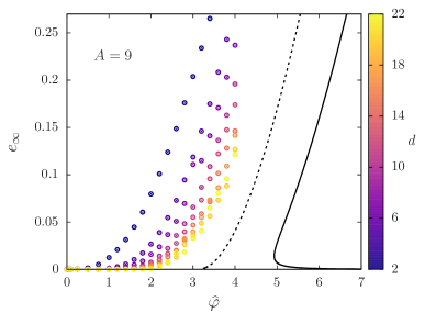
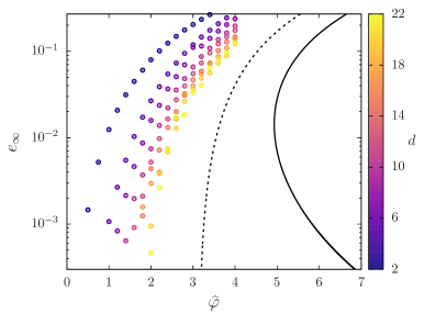
Figure 7: Numerical results for $e_{\infty}$ versus $\widehat{\varphi}$ in the RLG (same data as in Fig. 4(f), with cutoff $A=9$) compared with the Cugliandolo-Kurchan asymptotic prediction with one single time scale, using the marginal stability condition (full line), or the energy at which the solution for $\Delta$ disappears (dashed line). The left panel is in linear scale, while the right panel is in log-linear scale. Both predictions are inconsistent with the numerical results.

Some results are shown in Fig. 7. The full line is the Cugliandolo-Kurchan asymptotic prediction with one single time scale, i.e. the Monasson calculation at zero temperature given by Eqs. (136) and (137), together with the marginal stability condition $\lambda_{R}=0$ from Eq. (138). The curve is clearly not in agreement with the data, and is unphysically re-entrant at low energies. Replacing the condition of marginal stability with the energy at which the solution for $x$ in Eq. (136) disappears [82, 62] (dashed line) provides a qualitatively better result, but still inconsistent with the numerical results, and is dynamically unjustified (the line ends at $e_{\infty}$ at $\widehat{\varphi}_{J}=6.26$ as given in [80, 82]).

References

• Cugliandolo and Kurchan [1993] L. F. Cugliandolo and J. Kurchan, Analytical solution of the off-equilibrium dynamics of a long-range spin-glass model, Physical Review Letters 71, 173 (1993).
• Cugliandolo and Kurchan [1994] L. F. Cugliandolo and J. Kurchan, On the out-of-equilibrium relaxation of the Sherrington-Kirkpatrick model, Journal of Physics A: Mathematical and General 27, 5749 (1994).
• Cugliandolo [2003] L. F. Cugliandolo, Dynamics of glassy systems, in Slow relaxations and nonequilibrium dynamics in condensed matter, edited by J. Barrat, M. Feigelman, J. Kurchan, and J. Dalibard (Springer-Verlag, 2003) arXiv.org:cond-mat/0210312 .
• Barrat et al. [1997] A. Barrat, S. Franz, and G. Parisi, Temperature evolution and bifurcations of metastable states in mean-field spin glasses, with connections with structural glasses, Journal of Physics A: Mathematical and General 30, 5593 (1997).
• Montanari and Ricci-Tersenghi [2004] A. Montanari and F. Ricci-Tersenghi, Cooling-schedule dependence of the dynamics of mean-field glasses, Physical Review B 70, 134406 (2004).
• Rizzo [2013] T. Rizzo, Replica-symmetry-breaking transitions and off-equilibrium dynamics, Physical Review E 88, 032135 (2013).
• Folena et al. [2020] G. Folena, S. Franz, and F. Ricci-Tersenghi, Rethinking mean-field glassy dynamics and its relation with the energy landscape: The surprising case of the spherical mixed p-spin model, Physical Review X 10, 031045 (2020).
• Altieri et al. [2020] A. Altieri, G. Biroli, and C. Cammarota, Dynamical mean-field theory and aging dynamics, Journal of Physics A: Mathematical and Theoretical 53, 375006 (2020).
• Kurchan [2021] J. Kurchan, Time-reparametrization invariances, multithermalization and the Parisi scheme, arXiv:2101.12702  (2021).
• Baity-Jesi et al. [2019] M. Baity-Jesi, L. Sagun, M. Geiger, S. Spigler, G. B. Arous, C. Cammarota, Y. LeCun, M. Wyart, and G. Biroli, Comparing dynamics: deep neural networks versus glassy systems, Journal of Statistical Mechanics: Theory and Experiment 2019, 124013 (2019).
• Mannelli et al. [2019a] S. S. Mannelli, F. Krzakala, P. Urbani, and L. Zdeborova, Passed & spurious: Descent algorithms and local minima in spiked matrix-tensor models, in International conference on machine learning (PMLR, 2019) pp. 4333–4342.
• Mannelli et al. [2019b] S. S. Mannelli, G. Biroli, C. Cammarota, F. Krzakala, and L. Zdeborová, Who is afraid of big bad minima? analysis of gradient-flow in spiked matrix-tensor models, Advances in Neural Information Processing Systems 32, 8679 (2019b).
• Mannelli et al. [2020a] S. S. Mannelli, G. Biroli, C. Cammarota, F. Krzakala, P. Urbani, and L. Zdeborová, Complex dynamics in simple neural networks: Understanding gradient flow in phase retrieval, Advances in Neural Information Processing Systems 33, 3265 (2020a).
• Sclocchi and Urbani [2022] A. Sclocchi and P. Urbani, High dimensional optimization under non-convex excluded volume constraints, Phys. Rev. E 105, 024134 (2022).
• Biroli et al. [2020] G. Biroli, C. Cammarota, and F. Ricci-Tersenghi, How to iron out rough landscapes and get optimal performances: averaged gradient descent and its application to tensor pca, Journal of Physics A: Mathematical and Theoretical 53, 174003 (2020).
• Mannelli et al. [2020b] S. S. Mannelli, G. Biroli, C. Cammarota, F. Krzakala, P. Urbani, and L. Zdeborová, Marvels and pitfalls of the Langevin algorithm in noisy high-dimensional inference, Physical Review X 10, 011057 (2020b).
• Mignacco et al. [2021a] F. Mignacco, P. Urbani, and L. Zdeborová, Stochasticity helps to navigate rough landscapes: comparing gradient-descent-based algorithms in the phase retrieval problem, Machine Learning: Science and Technology 2, 035029 (2021a).
• Franz and Parisi [2016] S. Franz and G. Parisi, The simplest model of jamming, Journal of Physics A: Mathematical and Theoretical 49, 145001 (2016).
• Franz et al. [2017] S. Franz, G. Parisi, M. Sevelev, P. Urbani, and F. Zamponi, Universality of the sat-unsat (jamming) threshold in non-convex continuous constraint satisfaction problems, SciPost Physics 2, 019 (2017).
• Franz et al. [2019] S. Franz, S. Hwang, and P. Urbani, Jamming in multilayer supervised learning models, Physical Review Letters 123, 160602 (2019).
• Spigler et al. [2019] S. Spigler, M. Geiger, S. d’Ascoli, L. Sagun, G. Biroli, and M. Wyart, A jamming transition from under-to over-parametrization affects generalization in deep learning, Journal of Physics A: Mathematical and Theoretical 52, 474001 (2019).
• Franz et al. [2021] S. Franz, A. Sclocchi, and P. Urbani, Surfing on minima of isostatic landscapes: avalanches and unjamming transition, Journal of Statistical Mechanics: Theory and Experiment 2021, 023208 (2021).
• Mitchell et al. [1992] D. Mitchell, B. Selman, and H. Levesque, Hard and easy distributions of sat problems (1992).
• Kirkpatrick and Selman [1994] S. Kirkpatrick and B. Selman, Critical behavior in the satisfiability of random boolean expressions, Science 264, 1297 (1994).
• Monasson et al. [1999] R. Monasson, R. Zecchina, S. Kirkpatrick, B. Selman, and L. Troyansky, Determining computational complexity from characteristic ‘phase transitions’, Nature 400, 133 (1999).
• Altarelli et al. [2009] F. Altarelli, R. Monasson, G. Semerjian, and F. Zamponi, A review of the Statistical Mechanics approach to Random Optimization Problems, in Handbook of Satisfiability, Frontiers in Artificial Intelligence and Applications, edited by A. Biere, M. Heule, H. van Maaren, and T. Walsh (IOS Press, 2009) arXiv:0802.1829 .
• Folena et al. [2022] G. Folena, A. Manacorda, and F. Zamponi, Introduction to the dynamics of disordered systems: equilibrium and gradient descent, arXiv:0802.1829  (2022).
• Hwang and Ikeda [2020] S. Hwang and H. Ikeda, Force balance controls the relaxation time of the gradient descent algorithm in the satisfiable phase, Physical Review E 101, 052308 (2020).
• Gardner and Derrida [1988] E. Gardner and B. Derrida, Optimal storage properties of neural network models, Journal of Physics A: Mathematical and general 21, 271 (1988).
• Krauth and Mézard [1989] W. Krauth and M. Mézard, Storage capacity of memory networks with binary couplings, Journal de Physique 50, 3057 (1989).
• Brunel et al. [1992] N. Brunel, J.-P. Nadal, and G. Toulouse, Information capacity of a perceptron, Journal of Physics A: Mathematical and General 25, 5017 (1992).
• Monasson and Zecchina [1995] R. Monasson and R. Zecchina, Learning and generalization theories of large committee-machines, Modern Physics Letters B 9, 1887 (1995).
• Tikhonov and Monasson [2017] M. Tikhonov and R. Monasson, Collective phase in resource competition in a highly diverse ecosystem, Physical Review Letters 118, 048103 (2017).
• Landmann and Engel [2018] S. Landmann and A. Engel, Systems of random linear equations and the phase transition in MacArthur’s resource-competition model, EPL (Europhysics Letters) 124, 18004 (2018).
• Altieri and Franz [2019] A. Altieri and S. Franz, Constraint satisfaction mechanisms for marginal stability and criticality in large ecosystems, Physical Review E 99, 010401 (2019).
• De Martino et al. [2004] A. De Martino, M. Marsili, and I. P. Castillo, Statistical mechanics analysis of the equilibria of linear economies, Journal of Statistical Mechanics: Theory and Experiment 2004, P04002 (2004).
• Moran and Bouchaud [2019] J. Moran and J.-P. Bouchaud, May’s instability in large economies, Physical Review E 100, 032307 (2019).
• Sharma et al. [2021] D. Sharma, J.-P. Bouchaud, M. Tarzia, and F. Zamponi, Good speciation and endogenous business cycles in a constraint satisfaction macroeconomic model, Journal of Statistical Mechanics: Theory and Experiment 2021, 063403 (2021).
• Durian [1995] D. J. Durian, Foam mechanics at the bubble scale, Physical Review Letters 75, 4780 (1995).
• O’Hern et al. [2002] C. S. O’Hern, S. A. Langer, A. J. Liu, and S. R. Nagel, Random packings of frictionless particles, Physical Review Letters 88, 075507 (2002).
• O’Hern et al. [2003] C. S. O’Hern, L. E. Silbert, A. J. Liu, and S. R. Nagel, Jamming at zero temperature and zero applied stress: the epitome of disorder, Physical Review E 68, 011306 (2003).
• Liu and Nagel [2010] A. J. Liu and S. R. Nagel, The jamming transition and the marginally jammed solid, Annual Review of Condensed Matter Physics 1, 347 (2010).
• Liu et al. [2011] A. Liu, S. Nagel, W. Van Saarloos, and M. Wyart, The jamming scenario – an introduction and outlook, in Dynamical Heterogeneities and Glasses, edited by L. Berthier, G. Biroli, J.-P. Bouchaud, L. Cipelletti, and W. van Saarloos (Oxford University Press, 2011) arXiv:1006.2365 .
• Ikeda et al. [2020] A. Ikeda, T. Kawasaki, L. Berthier, K. Saitoh, and T. Hatano, Universal relaxation dynamics of sphere packings below jamming, Physical Review Letters 124, 058001 (2020).
• Nishikawa et al. [2021a] Y. Nishikawa, A. Ikeda, and L. Berthier, Relaxation dynamics of non-brownian spheres below jamming, Journal of Statistical Physics 182, 1 (2021a).
• Chacko et al. [2019] R. N. Chacko, P. Sollich, and S. M. Fielding, Slow coarsening in jammed athermal soft particle suspensions, Physical Review Letters 123, 108001 (2019).
• Nishikawa et al. [2021b] Y. Nishikawa, M. Ozawa, A. Ikeda, P. Chaudhuri, and L. Berthier, Relaxation dynamics in the energy landscape of glass-forming liquids, arXiv:2106.01755  (2021b).
• Sompolinsky and Zippelius [1981] H. Sompolinsky and A. Zippelius, Dynamic theory of the spin-glass phase, Physical Review Letters 47, 359 (1981).
• Sompolinsky and Zippelius [1982] H. Sompolinsky and A. Zippelius, Relaxational dynamics of the edwards-anderson model and the mean-field theory of spin-glasses, Physical Review B 25, 6860 (1982).
• Maimbourg et al. [2016] T. Maimbourg, J. Kurchan, and F. Zamponi, Solution of the dynamics of liquids in the large-dimensional limit, Physical Review Letters 116, 015902 (2016).
• Szamel [2017] G. Szamel, Simple theory for the dynamics of mean-field-like models of glass-forming fluids, Physical Review Letters 119, 155502 (2017).
• Agoritsas et al. [2018] E. Agoritsas, G. Biroli, P. Urbani, and F. Zamponi, Out-of-equilibrium dynamical mean-field equations for the perceptron model, Journal of Physics A: Mathematical and Theoretical 51, 085002 (2018).
• Agoritsas et al. [2019] E. Agoritsas, T. Maimbourg, and F. Zamponi, Out-of-equilibrium dynamical equations of infinite-dimensional particle systems. i. the isotropic case, Journal of Physics A: Mathematical and Theoretical 52, 144002 (2019).
• Liu et al. [2021] C. Liu, G. Biroli, D. R. Reichman, and G. Szamel, Dynamics of liquids in the large-dimensional limit, Physical Review E 104, 054606 (2021).
• Ikeda and Shimada [2020] H. Ikeda and M. Shimada, Vibrational density of states of jammed packing: mean-field theory and beyond, arXiv:2009.12060  (2020).
• Shimada et al. [2020] M. Shimada, H. Mizuno, L. Berthier, and A. Ikeda, Low-frequency vibrations of jammed packings in large spatial dimensions, Physical Review E 101, 052906 (2020).
• Franz et al. [2015] S. Franz, G. Parisi, P. Urbani, and F. Zamponi, Universal spectrum of normal modes in low-temperature glasses, Proceedings of the National Academy of Sciences 112, 14539 (2015).
• Lerner et al. [2013] E. Lerner, G. During, and M. Wyart, Low-energy non-linear excitations in sphere packings, Soft Matter 9, 8252 (2013).
• Ikeda [2020] H. Ikeda, Relaxation time below jamming, The Journal of Chemical Physics 153, 126102 (2020).
• Biroli et al. [2021a] G. Biroli, P. Charbonneau, E. I. Corwin, Y. Hu, H. Ikeda, G. Szamel, and F. Zamponi, Interplay between percolation and glassiness in the random Lorentz gas, Physical Review E 103, L030104 (2021a).
• Biroli et al. [2021b] G. Biroli, P. Charbonneau, Y. Hu, H. Ikeda, G. Szamel, and F. Zamponi, Mean-field caging in a random Lorentz gas, The Journal of Physical Chemistry B 125, 144 (2021b).
• Parisi et al. [2020] G. Parisi, P. Urbani, and F. Zamponi, Theory of simple glasses: exact solutions in infinite dimensions (Cambridge University Press, 2020).
• Manacorda et al. [2020] A. Manacorda, G. Schehr, and F. Zamponi, Numerical solution of the dynamical mean field theory of infinite-dimensional equilibrium liquids, The Journal of chemical physics 152, 164506 (2020).
• Bun et al. [2017] J. Bun, J.-P. Bouchaud, and M. Potters, Cleaning large correlation matrices: tools from random matrix theory, Physics Reports 666, 1 (2017).
• Arnoulx de Pirey et al. [2021] T. Arnoulx de Pirey, A. Manacorda, F. van Wijland, and F. Zamponi, Active matter in infinite dimensions: Fokker–planck equation and dynamical mean-field theory at low density, The Journal of Chemical Physics 155, 174106 (2021).
• Roy et al. [2019] F. Roy, G. Biroli, G. Bunin, and C. Cammarota, Numerical implementation of dynamical mean field theory for disordered systems: Application to the Lotka–Volterra model of ecosystems, Journal of Physics A: Mathematical and Theoretical 52, 484001 (2019).
• Mignacco et al. [2021b] F. Mignacco, F. Krzakala, P. Urbani, and L. Zdeborová, Dynamical mean-field theory for stochastic gradient descent in gaussian mixture classification, Journal of Statistical Mechanics: Theory and Experiment 2021, 124008 (2021b).
• Folena and Urbani [2021] G. Folena and P. Urbani, Marginal stability of soft anharmonic mean field spin glasses, arXiv:2106.16221  (2021).
• Mignacco and Urbani [2021] F. Mignacco and P. Urbani, The effective noise of stochastic gradient descent, arXiv:2112.10852  (2021).
• Charbonneau et al. [2015] P. Charbonneau, E. I. Corwin, G. Parisi, and F. Zamponi, Jamming criticality revealed by removing localized buckling excitations, Physical Review Letters 114, 125504 (2015).
• Mangeat and Zamponi [2016] M. Mangeat and F. Zamponi, Quantitative approximation schemes for glasses, Physical Review E 93, 012609 (2016).
• Charbonneau et al. [2021] P. Charbonneau, Y. Hu, J. Kundu, and P. K. Morse, The dimensional evolution of structure and dynamics in hard sphere liquids, arXiv:2111.13749  (2021).
• Sartor et al. [2021] J. D. Sartor, S. A. Ridout, and E. I. Corwin, Mean-field predictions of scaling prefactors match low-dimensional jammed packings, Physical Review Letters 126, 048001 (2021).
• Bouchaud [1992] J.-P. Bouchaud, Weak ergodicity breaking and aging in disordered systems, Journal de Physique I 2, 1705 (1992).
• Olsson and Teitel [2007] P. Olsson and S. Teitel, Critical Scaling of Shear Viscosity at the Jamming Transition, Physical Review Letters 99, 178001 (2007).
• Vagberg et al. [2011] D. Vagberg, P. Olsson, and S. Teitel, Glassiness, rigidity, and jamming of frictionless soft core disks, Physical Review E 83, 031307 (2011).
• Olsson and Teitel [2020] P. Olsson and S. Teitel, Dynamic length scales in athermal, shear-driven jamming of frictionless disks in two dimensions, Phys. Rev. E 102, 042906 (2020).
• Mari et al. [2009] R. Mari, F. Krzakala, and J. Kurchan, Jamming versus glass transitions, Physical Review Letters 103, 025701 (2009).
• Mari and Kurchan [2011] R. Mari and J. Kurchan, Dynamical transition of glasses: from exact to approximate, The Journal of Chemical Physics 135, 124504 (2011).
• Parisi and Zamponi [2010] G. Parisi and F. Zamponi, Mean-field theory of hard sphere glasses and jamming, Reviews of Modern Physics 82, 789 (2010).
• Ozawa et al. [2017] M. Ozawa, L. Berthier, and D. Coslovich, Exploring the jamming transition over a wide range of critical densities, SciPost Physics 3, 027 (2017).
• Berthier et al. [2011] L. Berthier, H. Jacquin, and F. Zamponi, Microscopic theory of the jamming transition of harmonic spheres, Physical Review E 84, 051103 (2011).
• Scalliet et al. [2019] C. Scalliet, L. Berthier, and F. Zamponi, Marginally stable phases in mean-field structural glasses, Physical Review E 99, 012107 (2019).
• Monasson [1995] R. Monasson, Structural glass transition and the entropy of the metastable states, Physical Review Letters 75, 2847 (1995).
• Wyart [2012] M. Wyart, Marginal stability constrains force and pair distributions at random close packing, Physical Review Letters 109, 125502 (2012).
• Müller and Wyart [2015] M. Müller and M. Wyart, Marginal stability in structural, spin, and electron glasses, Annual Review of Condensed Matter Physics 6, 177 (2015).
• Montanari and Ricci-Tersenghi [2003] A. Montanari and F. Ricci-Tersenghi, On the nature of the low-temperature phase in discontinuous mean-field spin glasses, The European Physical Journal B 33, 339 (2003).
• Charbonneau et al. [2014a] P. Charbonneau, J. Kurchan, G. Parisi, P. Urbani, and F. Zamponi, Exact theory of dense amorphous hard spheres in high dimension. III. The full replica symmetry breaking solution, Journal of Statistical Mechanics: Theory and Experiment 2014, P10009 (2014a).
• Charbonneau et al. [2014b] P. Charbonneau, J. Kurchan, G. Parisi, P. Urbani, and F. Zamponi, Fractal free energies in structural glasses, Nature Communications 5, 3725 (2014b).
• Bernaschi et al. [2020] M. Bernaschi, A. Billoire, A. Maiorano, G. Parisi, and F. Ricci-Tersenghi, Strong ergodicity breaking in aging of mean-field spin glasses, Proceedings of the National Academy of Sciences 117, 17522 (2020).
• [91] G. Folena, private communication.