On the origin of Field-Induced Boson Insulating States in a 2D Superconducting Electron Gas with Strong Spin-Orbit Scatterings

Abstract

We search for the deep origin of the field-induced superconductor-to-insulator transitions observed experimentally in electron-doped SrTiO₃/LaAlO₃ interfaces, which were analyzed theoretically very recently within the framework of superconducting fluctuations approach (Phys. Rev. B 104, 054503 (2021)). Employing the 2D electron-gas model with strong spin-orbit scatterings, we have found that in the zero temperature limit, field-induced unbounded growth of the fluctuation mass, and consequent divergence of Cooper-pair density in mesoscopic puddles, drives the system to Boson insulating states at high fields. Application of this model to the gate-voltage tuned 2D electron system, created in the SrTiO₃/LaAlO₃ (111) interface at low temperatures, shows that, at sufficiently high fields, the DOS conductivity prevails over the paraconductivity, resulting in strongly enhanced magnetoresistance in systems with sufficiently small carriers density. Dynamical quantum tunneling of Cooper pairs breaking into mobile normal-electrons states, which prevent the divergence at zero temperature, contain the high-field resistance onset.

In a very recent paper MZPRB2021 we have shown that Cooper-pair fluctuations in a 2D electron gas with strong spin-orbit scatterings can lead at low temperatures to pronounced magnetoresistance (MR) peaks above a crossover field to superconductivity. The model was applied to the high mobility electron systems formed in the electron-doped interfaces between two insulating perovskite oxides—SrTiO₃ and LaAlO₃ Ohtomo04 , showing good quantitative agreement with a large body of experimental sheet-resistance data obtained under varying gate voltage Mograbi19 .

The model employed was based on the opposing effects generated by fluctuations in the superconducting (SC) order parameter: The nearly singular enhancement of conductivity (paraconductivity) due to fluctuating Cooper pairs below the nominal (mean-field) critical magnetic field, on one hand, and the suppression of conductivity, associated with the loss of unpaired electrons due to Cooper pairs formation, on the other hand. The self-consistent treatment of the interaction between fluctuations UllDor90 ,UllDor91 , employed in these calculations, avoids the critical divergence of both the Aslamazov-Larkin (AL) paraconductivity AL68 and the DOS conductivity LV05 , allowing to extend the theory to regions well below the nominal critical SC transition. The absence of long range phase coherence implied by this approach is consistent with the lack of the ultimate zero-resistance state in the entire data analyzed there.

In the present paper we focus our attention on the most intriguing question arising from the Cooper-pair fluctuations scenario of the superconductor–insulator transition (SIT) presented in Ref.MZPRB2021 , that is how Cooper-pairs liquid, whose condensation (in momentum space) is customarily associated with superconductivity, could metamorphose into an insulator just by lowering its temperature under sufficiently high magnetic field ? We have already identified the highly suppressed normal-state DOS due to Cooper-pairs formation as the dominant origin of the insulator side of the SIT.

Here we show that field-induced vanishing of the fluctuations stiffness in the zero temperature limit is at the core of this intriguing phenomenon. Under these extreme circumstances, the fluctuation mass enhances without limit, the AL paraconductivity vanishes and the DOS conductivity diverges, so that at low but finite temperature the DOS conductivity prevails over the AL conductivity at fields that roughly indicate the presence of the observed enhanced MR.

It is therefore concluded that the consequent divergence of the Cooper-pairs density within mesoscopic puddles, as predicted by the thermal fluctuations approach in the zero temperature limit, should bolster dynamical quantum tunneling of Cooper pairs breaking into unpaired mobile electrons states, and so containing the resistance onset. This feature reflects on the overall comparison process with the experimental data, which shows selective sensitivity to the phenomenological parameters determining both the rate of quantum tunneling and the normal-state conductivity.

I Conductance fluctuations in the zero temperature limit

In order to reveal the origin of the puzzling insulating state that emerges in our approach from SC fluctuations we will consider in this section the fluctuations contributions to the sheet conductivity in the magnetic fields region where they are rigorously derivable from the microscopic Gor’kov Ginzburg-Landau theory, i.e. above the nominal (mean-field) critical field, determined from the vanishing of the Gaussian critical shift-parameter MZPRB2021 :

$$\varepsilon_{H}\equiv\ln\left(\frac{T}{T_{c0}}\right)+a_{+}\psi\left(\frac{1}{2}+f_{-}\right)+a_{-}\psi\left(\frac{1}{2}+f_{+}\right)-\psi\left(1/2\right)$$ (1)

Here $T_{c0}$ is the mean-field SC transition temperature at zero magnetic field, $\psi$ is the digamma function, $\ f_{\pm}=\delta H^{2}+\beta\pm\sqrt{\beta^{2}-\mu^{2}H^{2}}$, $a_{\pm}=\left(1\pm\beta/\sqrt{\beta^{2}-\mu^{2}H^{2}}\right)/2$ are dimensionless functions of the magnetic field $H$, with the basic parameters: $\ \beta\equiv\varepsilon_{SO}/4\pi k_{B}T,$ $\mu\equiv\mu_{B}/2\pi k_{B}T,$ $\delta\equiv D\left(de\right)^{2}/2\pi k_{B}T\hslash$, where $D\equiv\hbar E_{F}/m^{\ast}\varepsilon_{SO}$ the electron diffusion coefficient, and $\varepsilon_{SO}=\hbar/\tau_{SO}$ is the spin-orbit energy. There are no restrictions on the temperature $T$ as we are mainly interested in the low temperatures region well below $T_{c0}$ down to the limit of $T\rightarrow 0$.

I.1 DOS conductivity

As indicated in MZPRB2021 , the phenomenological approach to the calculation of the DOS conductivity, based on the simple Drude formula: $\delta\sigma_{DOS}=-2n_{s}e^{2}\tau_{SO}/m^{\ast}$, as first introduced by Larkin and Varlamov LV05 for the zero-field case in the dirty limit, can fit nicely the result derived by means of a fully microscopic (diagrammatic) approach. The key factor is the Cooper-pair fluctuations number density $n_{s}$:

$$n_{s}=\frac{1}{d}\frac{1}{\left(2\pi\right)^{2}}\int\left\langle\left|\psi\left(q\right)\right|^{2}\right\rangle d^{2}q$$ (2)

which depends on an appropriate selection of its momentum distribution function: $\left\langle\left|\psi\left(q\right)\right|^{2}\right\rangle$.  The latter was selected by generalizing the pure-limit zero-field expression LV05 : $\left\langle\left|\psi\left(q\right)\right|^{2}\right\rangle=\alpha^{-1}\left[\ln\left(T/T_{c0}\right)+\xi^{2}q^{2}\right]^{-1},$ with:$\ \alpha=4\pi^{2}k_{B}T/7\zeta\left(3\right)E_{F}$, $\zeta\left(3\right)\simeq 1.202$, and $\xi=\hbar v_{F}/2\pi k_{B}T$, to the dirty-limit finite-field expression:

$$\left\langle\left|\psi\left(q\right)\right|^{2}\right\rangle\simeq\frac{7\zeta\left(3\right)E_{F}}{4\pi^{2}k_{B}T}\frac{1}{\Phi\left(x;\varepsilon_{H}\right)}$$ (3)

where:

$$\Phi\left(x;\varepsilon_{H}\right) = \varepsilon_{H}+a_{+}\left[\psi\left(1/2+f_{-}+x\right)-\psi\left(1/2+f_{-}\right)\right]$$ (4)

$$+a_{-}\left[\psi\left(1/2+f_{+}+x\right)-\psi\left(1/2+f_{+}\right)\right]$$

and $x=\hbar Dq^{2}/4\pi k_{B}T$.  The resulting expression of the DOS conductivity contribution is given by:

$$\delta\sigma_{DOS}d\simeq-3.5\zeta\left(3\right)\left(\frac{G_{0}}{\pi}\right)\int_{0}^{x_{c}}\frac{dx}{\Phi\left(x;\varepsilon_{H}\right)}$$ (5)

where $G_{0}=e^{2}/\pi\hbar$ is the conductance quantum, $x_{c}=\hbar Dq_{c}^{2}/4\pi k_{B}T$, with $q_{c}$ the cutoff wave number, and $3.5\zeta\left(3\right)\simeq 4.207$.

Further insight into the zero-temperature limit of $\delta\sigma_{DOS}d$ is gained by exploiting the linear approximation of Eq.(4), i.e.:  $\Phi\left(x;\varepsilon_{H}\right)\simeq\varepsilon_{H}+\eta\left(H\right)x$, where:

$$\eta\left(H\right)=a_{+}\psi^{\prime}\left(\frac{1}{2}+f_{-}\right)+a_{-}\psi^{\prime}\left(\frac{1}{2}+f_{+}\right)$$ (6)

and performing the integration over $x$ analytically, which yields:

$$\delta\sigma_{DOS}d\simeq-3.5\zeta\left(3\right)\left(\frac{G_{0}}{\pi}\right)\frac{1}{\eta\left(H\right)}\ln\left(1+\frac{\eta\left(H\right)x_{c}}{\varepsilon_{H}}\right)$$ (7)

In the zero field limit ( $\eta\left(H\rightarrow 0\right)=\psi^{\prime}\left(1/2\right)=\pi^{2}/2\equiv\eta$), and for sufficiently large cutoff, i.e. $x_{c}\gg\varepsilon_{H}/\eta\left(H\right)$, we find:  $\delta\sigma^{DOS}\left(H\rightarrow 0\right)\simeq-3.5\zeta\left(3\right)\left(\frac{G_{0}}{\pi d\eta}\right)\ln\frac{\eta x_{c}}{\varepsilon}$, so that:

$$\delta\sigma^{DOS}\simeq-\left(\frac{7\zeta\left(3\right)}{\pi^{4}}\right)\left(\frac{e^{2}}{d\hbar}\right)\ln\left(\frac{\eta x_{c}}{\varepsilon}\right)$$

in complete agreement footnote1 with the result of a fully microscopic (diagrammatic) approach presented in Appendix A (Eq.23) for a 2D system, following the method used in Ref.LV05 for a layered superconductor.

I.2 Paraconductivity

The AL contribution to the sheet conductance derived in Ref.MZPRB2021 was obtained from the retarded current-current correlator:

$$Q_{AL}^{R}\left(\omega\right)=k_{B}T\left(\frac{2e}{\hbar}\right)^{2}\left(\frac{1}{2\pi d}\right)\int\limits_{0}^{x_{c}}xdx$$ (8)

$$\sum\limits_{n=0,\pm 1,\pm 2,....}\frac{\Phi^{\prime}\left(x+\left|n+y\right|;\varepsilon_{H}\right)}{\Phi\left(x+\left|n+y\right|;\varepsilon_{H}\right)}\frac{\Phi^{\prime}\left(x+\left|n\right|;\varepsilon_{H}\right)}{\Phi\left(x+\left|n\right|;\varepsilon_{H}\right)}$$

where $y=i\hbar\omega/2\pi k_{B}T$, and $\omega$ is the frequency of the response function.

Using Eq.8 all nonzero Matsubara-frequency terms in the corresponding AL static conductivity $\sigma_{AL}=\lim_{\omega\rightarrow 0}\left(i/\omega\right)\left[Q_{AL}^{R}\left(\omega\right)-Q_{AL}^{R}\left(0\right)\right]$ are canceled out and the remaining $n=0$ term can be written in the form:

$$\sigma_{AL}d=\frac{1}{4}\left(\frac{G_{0}}{\pi}\right)\int\limits_{0}^{x_{c}}\left(\frac{\Phi^{\prime}\left(x;\varepsilon_{H}\right)}{\Phi\left(x;\varepsilon_{H}\right)}\right)^{2}dx$$ (9)

Exploiting the linear approximation of Eq.(4), i.e.:  $\Phi\left(x;\varepsilon_{H}\right)\simeq\varepsilon_{H}+\eta\left(H\right)x$, and performing the integration over $x$ analytically we find:

$$\sigma_{AL}d\simeq\frac{1}{4}\left(\frac{G_{0}}{\pi}\right)\frac{\eta\left(H\right)}{\varepsilon_{H}\left(1+\frac{\varepsilon_{H}}{\eta\left(H\right)x_{c}}\right)}$$ (10)

I.3 Infinite boson mass at zero temperature

Combining Eq.(7) with Eq.(10), the total fluctuations contributions to the sheet conductance is written as:

$$\sigma^{fluct}d\simeq\left(\frac{G_{0}}{\pi}\right)\left[\frac{\eta\left(H\right)}{4}\frac{1}{\varepsilon_{H}\left(1+\frac{\varepsilon_{H}}{\eta\left(H\right)x_{c}}\right)}\right.$$

$$\left.-\frac{3.5\zeta\left(3\right)}{\eta\left(H\right)}\ln\left(1+\frac{\eta\left(H\right)x_{c}}{\varepsilon_{H}}\right)\right]$$ (11)

which highlights the complementary roles played by the stiffness parameter $\eta\left(H\right)$ in the AL and DOS conductivities. The importance of $\eta\left(H\right)$ in controlling the development of an insulating bosonic state at low temperatures and high magnetic field can be clearly understood by considering the extreme situation of its zero temperature limit.

To effectively investigate this limiting situation it will be helpful to rewrite $\eta\left(H\right)$ as a sum over fermionic Matzubara frequency, that is:

$$\eta\left(h\right)=\sum\limits_{n=0}^{\infty}\frac{\left(n+1/2+2\beta+\overline{\delta}h^{2}\right)^{2}-\overline{\mu}^{2}h^{2}}{\left[\left(n+1/2+\overline{\delta}h^{2}\right)\left(n+1/2+2\beta+\overline{\delta}h^{2}\right)+\overline{\mu}^{2}h^{2}\right]^{2}}$$ (12)

where: $h\equiv H/H_{c\parallel 0}^{\ast},t\equiv T/T_{c}^{\ast},\beta=\beta_{0}/t,\overline{\mu}=\mu_{0}/t,\overline{\delta}=\delta_{0}/t,\beta_{0}\equiv\varepsilon_{SO}/4\pi k_{B}T_{c}^{\ast},\delta_{0}\equiv D\left(deH_{c\parallel 0}^{\ast}\right)^{2}/2\pi k_{B}T_{c}^{\ast}\hslash,$

$\mu_{0}\equiv\mu_{B}H_{c\parallel 0}^{\ast}/2\pi k_{B}T_{c}^{\ast}$, with $H_{c\parallel 0}^{\ast}$ and $T_{c}^{\ast}$ being characteristic scales of the critical parallel magnetic field and critical temperature, respectively.

In the zero temperature ($t\rightarrow 0$) limit, at finite magnetic field, $h>0$, the discrete summation in Eq.(12) transforms into integration, i.e.: $\ \eta\left(h\right)\rightarrow t\int\limits_{0}^{\infty}d\nu\frac{\left(\nu+2\beta_{0}+\delta_{0}h^{2}\right)^{2}-\mu_{0}^{2}h^{2}}{\left[\left(\nu+\delta_{0}h^{2}\right)\left(\nu+2\beta_{0}+\delta_{0}h^{2}\right)+\mu_{0}^{2}h^{2}\right]^{2}}=t\frac{1}{h^{2}}\frac{\delta_{0}h^{2}+2\beta_{0}}{h^{2}\delta_{0}^{2}+2\beta_{0}\delta_{0}+\mu_{0}^{2}}$, so that:

$$\eta\left(h\right)\rightarrow t\left(\frac{\eta_{0}\left(h\right)}{h^{2}}\right)\rightarrow 0$$ (13)

where:

$$\eta_{0}\left(h\right)\equiv\frac{\delta_{0}h^{2}+2\beta_{0}}{\left(\delta_{0}h^{2}+2\beta_{0}\right)\delta_{0}+\mu_{0}^{2}}$$ (14)

Note that at zero magnetic field: $\eta\left(h=0\right)=\sum_{n=0}^{\infty}\left(n+1/2\right)^{-2}=\psi^{\prime}\left(1/2\right)=\pi^{2}/2$, independent of temperature.

Thus, the zero temperature limit of the sheet conductance, Eq.(11), at fields above the nominal critical field $H_{c\parallel 0}^{\ast}$ can be written in the form:

$$\left(\sigma^{fluct}\right)_{h>1,t\rightarrow 0}d\rightarrow\left(\frac{G_{0}}{\pi}\right)\left[t\left(\frac{\eta_{0}\left(h\right)}{4h^{2}}\right)\frac{1}{\varepsilon_{h}\left(1+\frac{h^{2}\varepsilon_{h}}{\eta_{0}\left(h\right)x_{0}}\right)}\right.$$

$$\left.-\frac{1}{t}\left(\frac{3.5\zeta\left(3\right)h^{2}}{\eta_{0}\left(h\right)}\right)\ln\left(1+\frac{\eta_{0}\left(h\right)x_{0}}{h^{2}\varepsilon_{h}}\right)\right]$$ (15)

where $x_{0}\equiv\hbar Dq_{c}^{2}/4\pi k_{B}T_{c}^{\ast}$ is the temperature-independent cutoff parameter. It should be stressed at this point that the temperature-independent argument of the logarithmic factor in Eq.(15) (see Ref.footnote2 ) is consistent with the temperature-dependent cutoff parameter $x_{c}=x_{0}/t$.

Thus, we conclude that in the $t\rightarrow 0$ limit the AL paraconductivity follows the vanishing stiffness parameter $\eta\left(h\right)\propto t$, Eq.(13), whereas the DOS conductivity diverges with $1/\eta\left(h\right)\propto 1/t$. The former effect is a direct consequence of the divergent effective mass of the fluctuations, whereas the latter is due to the unlimited accumulation of Cooper-pairs within fluctuation puddles, whose characteristic spatial size:

$$\xi\left(t\rightarrow 0\right)=\left(\frac{\eta_{0}\left(h\right)}{h^{2}\varepsilon_{h}}\frac{\hbar D}{4\pi k_{B}T_{c}^{\ast}}\right)^{1/2}$$

remains finite in this extreme limiting situation. The decreasing asymptotic field dependence ($\eta\left(h\right)\propto 1/h^{2}$) of the stiffness parameter (see Eq.(13)) further enhances the sheet resistance at high fields by diminishing the localization length ($\xi\left(t\rightarrow 0\right)\propto 1/h\sqrt{\varepsilon_{h}}$).

II Quantum tunneling and pair breaking in the boson-insulating state

It is evident that, in light of the limited number of unpaired electrons available for the total conductivity, the ultimately divergent negative conductance implied by Eq.(15) is an unphysical result, which clearly indicates the nature of the correction introduced in Ref.MZPRB2021 . In particular, the limitlessly rising Cooper-pairs density within mesoscopic puddles, predicted by Eq.(15) in the zero temperature limit, can be stopped only by allowing the superfluous Cooper pairs to tunnel out of the puddles while breaking into unpaired mobile electron states. This should prevent the vanishing of the total conductivity and the consequent divergence of the sheet resistance at high fields.

The formal incorporation of such a quantum correction into the thermal conductance fluctuation, which was made in Ref. MZPRB2021 , amounts to multiplying the AL term in Eq.(11) by the factor $\left(1+T_{Q}/T\right)$, where $T_{Q}$ stands for the tunneling attempt rate, and dividing the DOS conductivity term by the same factor (see Appendix B for the physical motivation). In parallel with these external corrections, the electron pairing functions $\varepsilon_{H}$ and $\eta\left(H\right)$ appearing in Eq.(11) were modified by inserting the frequency-shift term $T_{Q}/2T$ to the arguments of the digamma functions and their derivatives in Eq.(1) and Eq.(6) respectively (see Appendix B for more details). The external corrections are equivalent to replacing the stiffness parameter appearing in the prefactors of the AL and the DOS terms in Eq.(11) with the hybrid expression:

$$\eta\left(H\right)\rightarrow\left(1+\frac{T_{Q}}{T}\right)\eta_{U}\left(h\right)$$ (16)

where $\eta_{U}\left(h\right)$ is obtained from $\eta\left(h\right)$ in Eq.(12) by inserting, under the Fermion Matsubara frequency summation, the frequency-shift term $T_{Q}/2T$ :

$$\eta_{U}\left(h\right)=\sum\limits_{n=0}^{\infty}$$ (17)

$$\frac{\left(n+1/2+T_{Q}/2T+2\beta+\overline{\delta}h^{2}\right)^{2}-\overline{\mu}^{2}h^{2}}{\left[\left(n+1/2+T_{Q}/2T+\overline{\delta}h^{2}\right)\left(n+1/2+T_{Q}/2T+2\beta+\overline{\delta}h^{2}\right)+\overline{\mu}^{2}h^{2}\right]^{2}}$$

In Eq.(16), $\left({\normalsize 1+T_{Q}/T}\right)$ represents the effect of quantum tunneling of Cooper pairs, whereas the frequency-shift term $T_{Q}/2T$ appearing in Eq.(17) for $\eta_{U}\left(h\right)$, represents pair-breaking effect associated with the tunneling process.

The corresponding pair-breaking effect on the critical-shift parameter results in transforming $\varepsilon_{H}$ according to:

$$\varepsilon_{H} \rightarrow \varepsilon_{h}^{U}\equiv\ln\left(\frac{T}{T_{c0}}\right)+a_{+}\psi\left(\frac{1}{2}+T_{Q}/2T+f_{-}\right)$$

$$+a_{-}\psi\left(\frac{1}{2}+T_{Q}/2T+f_{+}\right)-\psi\left(1/2\right)$$

In the absence of quantum tunneling $\varepsilon_{H}$ (Eq.(1)) is subjected to the usual magnetic field induced pair-breaking effect ShahLopatin07 through either the Zeeman spin-splitting energy ($\mu_{B}H$), or/and the diamagnetic energy ($D\left(deH\right)^{2}/\hslash$) terms. In the zero temperature limit, the effect is dramatically reflected in the removal of the (Cooper) singularity of the logarithmic term in Eq.(1), due to exact cancellation by the asymptotic values of the digamma functions for $\ f_{\pm}\gg 1$ (see Appendix C). In the presence of quantum tunneling, the excitation frequency shift $\pi k_{B}$$T_{Q}/\hbar$ introduced to define $\varepsilon_{h}^{U}$, Eq.(II), causes in this limit an additional, field-independent pair-breaking effect through the asymptotic behavior of the digamma functions for $T_{Q}/2T\gg 1$ (see Appendix C).

For systems with long range phase coherence described, e.g. in Ref.ShahLopatin07 , Lopatinetal05 the main impact of the pair-breaking perturbations is near the critical point $\varepsilon_{H}=0$ for Cooper pairs condensation (at $q=0)$ in momentum space. For the system of strong SC fluctuations at very low temperatures, under consideration here, where Cooper pairs tend to condense within mesoscopic puddles in real space, and their excitation process associated with the frequency shift $\pi k_{B}T_{Q}/\hbar$  greatly disperse in momentum space, dynamical quantum tunneling, which is inherently connected to this excitation process, strongly reinforces pair-breaking processes into unpaired electron states.

The sharp plunge of $\eta\left(h\right)$ just above $h=0$ for $T\rightarrow 0$, discussed below Eq.(13) (see Fig.1), is a reflection in the stiffness parameter of the field-induced pair-breaking effect. As indicated above, the frequency shift that transforms $\eta\left(h\right)$ to $\eta_{U}\left(h\right)$, and represents field-independent pair breaking effect, is intimately connected to the quantum tunneling process discussed above. This is clearly seen by considering the zero temperature limit of $\eta_{U}\left(h\right)$ in Eq.(17):

$$\left(\eta_{U}\left(h\right)\right)_{T\rightarrow 0}=\left(\frac{T}{T_{Q}}\right)_{T\rightarrow 0}\eta_{Q}\left(h\right)$$ (19)

where:

$$\eta_{Q}\left(h\right)\equiv$$

$$\int\limits_{0}^{\infty}d\nu\frac{\left(\nu+1/2+2\beta_{Q}+\delta_{Q}h^{2}\right)^{2}-\mu_{Q}^{2}h^{2}}{\left[\left(\nu+1/2+\delta_{Q}h^{2}\right)\left(\nu+1/2+2\beta_{Q}+\delta_{Q}h^{2}\right)+\mu_{Q}^{2}h^{2}\right]^{2}}$$

$$=\frac{1}{h^{2}}\frac{\delta_{Q}h^{2}+2\beta_{Q}}{h^{2}\delta_{Q}^{2}+2\beta_{Q}\delta_{Q}+\mu_{Q}^{2}}$$ (20)

and: $\beta_{Q}=\beta_{0}/t_{Q},\mu_{Q}=\mu_{0}/t_{Q},\delta_{Q}=\delta_{0}/t_{Q},t_{Q}\equiv T_{Q}/T_{c}^{\ast}$.

The limiting function $\eta_{Q}\left(h\right)$ in Eq.(II) is a continuous smooth function of the field $h$, including at $h=0$.  Therefore, Eq.(19) implies that the discontinuous plunge of $\eta\left(h\right)$ at $h=0$ in the zero temperature limit is removed by the frequency shift term, as can be directly checked in Eq.(17). The overall magnitude of $\eta_{U}\left(h\right)$ diminishes to zero with $T/T_{Q}$ in this limit. However, by multiplying with the divergent quantum tunneling factor $\left(1+T_{Q}/T\right)$ the resulting hybrid product in Eq.(16), which represents the combined effect of quantum tunneling and pair breaking, is a smooth finite function of the field $\eta_{Q}\left(h\right)$ (see Fig.1).

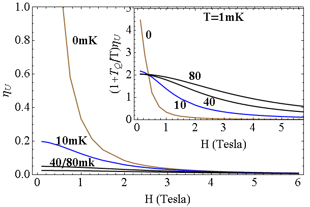
Figure 1: Field-dependent stiffness parameter $\eta_{U}\left(H\right)$ calculated at $T=1$ mK for $T_{Q}=0,10,40,80$ mK. Inset: The hybrid product $\left(1+T_{Q}/T\right)\eta_{U}\left(H\right)$ calculated for the same $T$ and $T_{Q}$ values as presented in the main figure.

Our self-consistent field (SCF) approach, exploited in Ref.MZPRB2021 for calculating the critical-shift parameter $\widetilde{{\normalsize\varepsilon}}_{H}$ in the presence of interaction between Gaussian fluctuations, avoids the critical divergence of both the AL paraconductivity and the DOS conductivity, and allows to extend Eq.(11) for the conductance fluctuations to regions well below the nominal critical SC transition. It also offers an extended proper measure of the pair-breaking effect. In contrast to $\varepsilon$_H, $\widetilde{{\normalsize\varepsilon}}_{H}$ is positive definite in the entire fields range, including that below the critical field where $\varepsilon$${}_{H}<0$ (see Fig.2). The uniform enhancement of $\widetilde{{\normalsize\varepsilon}}$${}_{H}^{U}$ with respect to $\widetilde{{\normalsize\varepsilon}}_{H}$, seen in Fig.2, resulting from the introduction of the frequency shift to the SCF equation (see Ref.MZPRB2021 ), is a genuine measure of the pair-breaking effect associated with the frequency shift. Its monotonically increasing field dependence seen in Fig.2 properly reflects the field-induced pair-breaking effect in the entire fields range.

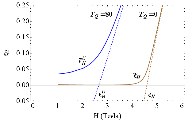
Figure 2: Field dependence, at $T=30$ mK, of the "bare" critical-shift parameter $\varepsilon_{H}^{U}$ (dashed lines), and the corresponding self-consistently "dressed" parameter $\widetilde{\varepsilon}_{H}^{U}$ (solid lines), in the absence of quantum tunneling (brown curves) and for $T_{Q}=80$ mK (blue curves).  Note the downward shift of the critical field and the uniform enhancement of the dressed critical-shift parameter associated with the quantum tunneling effect.

III Sensitivity tests of the fitting process

Practically speaking, the quantum tunneling introduced into the thermal fluctuations theory–an essential requirement for avoiding the unphysical divergence of the high-field DOS conductivity at zero temperature, and the normal-electron conductivity term, which is closely related to the pair-breaking processes bound to the tunneling events, are both phenomenological constituents of our model, which are exclusively determined by the experimental sheet-resistance data reported in Ref.Mograbi19 .

The other parameters in this model have microscopic origins and so can either be evaluated from first principles or be extracted independently from (other) experiments. Among the former group of microscopic parameters the numerical prefactor of the total fluctuations conductance given by Eq.(11) can be checked versus the relevant literature LV05 . At zero field, where the stiffness parameter $\eta\left(h=0\right)=\pi^{2}/2$, is independent of the spin-orbit energy parameter $\beta_{0}$, and the corresponding conductance is:

$$\sigma^{fluct}\left(H=0\right)\simeq\left(\frac{e^{2}}{\hbar d}\right)\left[\left(\frac{1}{8}\right)\frac{1}{\varepsilon}-\left(\frac{7\zeta\left(3\right)}{\pi^{4}}\right)\ln\left(\frac{\pi^{2}x_{c}}{2\varepsilon}\right)\right]$$ (21)

the prefactor is found here to be twice larger than that reported in Ref.LV05 . While we have not been able so far to successfully trace back to the origin of this discrepancy such a variation in the amplitude of the total (AL plus DOS) fluctuations conductivity is not expected to significantly change the results of the fitting process presented in Ref. MZPRB2021 . As will be elaborated below, the results of the fitting process can exactly be reproduced by slightly readjusting only the two phenomenological parameters of the theory:–the tunneling attempt rate, $T_{Q}\left(T,H\right)$, and the normal-state conductivity, $\sigma_{n}\left(H,T\right).$

An important parameter in the fitting process is the magnetic field $H_{\max}$ at which the sheet resistance has its maximum:– the outstanding feature characterizing the emergence of the insulating state at low temperatures. This parameter is predominantly determined by the location of the minimum $H_{\min}$ of the fluctuations conductivity $\sigma^{fluct}\left(H,T\right)$, but is slightly shifted downward due to the field dependence (increasing with increasing field) of the normal state conductivity $\sigma_{n}$$\left(H,T\right)$. In the absence of quantum tunneling, $\sigma^{fluct}\left(H,T\right)$ at very low temperature exhibits an asymmetrical sharp minimum arising from the opposing effects of the sharply diminishing AL term with increasing field above the nominal (mean-field) critical point and the less sharply decreasing DOS conductivity term in Eq.(11). The relevant field dependencies of these terms above the nominal critical point are controlled by the field dependencies of $\eta\left(h\right)$ and $\varepsilon$_h, as shown in Figs.1 and 2, respectively. The dimensionless spin-orbit energy parameter $\beta_{0}$ exclusively determines $H_{\min}$ in the absence of quantum tunneling. The dependence of $H_{\max}$ on the gate voltage shown in Fig.3 is therefore conveyed through the dependence of $\beta_{0}$ on the Fermi energy $E_{F}$.

Allowing for quantum tunneling of Cooper pairs, with attempt rate $T_{Q}$, the sharp minimum of $\sigma^{fluct}\left(H,T\right)$ is smeared, and due to the asymmetry of the latter, $H_{\min}$ is shifted downward (see Fig.4). The corresponding shift of $H_{\max}$, in conjunction with the downward shift associated with the field dependence of $\sigma_{n}$$\left(H,T\right)$, enable us fitting the data by exclusively varying the phenomenological parameters $T_{Q}\left(H,T\right)$ and $\sigma_{n}$$\left(H,T\right)$, without changing the other parameters. Note that, in contrast to $H_{\min}$ which shifts downward with decreasing $\beta_{0}$ (or $E_{F}$), the depths of the minima in Fig.4 are seen to be independent of $\beta_{0}$.   Consequently, the high-field tails of $\sigma^{fluct}\left(H,T\right)$ for the smaller value of $\beta_{0}$ shown in Fig.4, which always lay below zero, are seen to situate above the corresponding tails for the larger value of $\beta_{0}$. To compensate for these negative values, the field independent normal-state conductivity parameter in our fitting process, $\sigma_{0}\left(T\right)$, should be smaller for smaller values of $\beta_{0}$ (as indeed found, see Table I). This feature reflects the underlying consistency of our fluctuations approach (through the dependence of $\sigma^{fluct}\left(H,T\right)$ upon the normal-state carrier density) with the experimentally observed high-field resistance (through its dependence on the gate voltage).

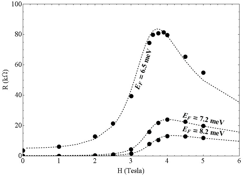
Figure 3: Measured sheet resistance at $T=30$ mK, as a function of field for three gate voltages (corresponding to $R_{N}=20.5,10.5,7.5$ k$\Omega$) as reported in Ref. Mograbi19 (full circles). The dashed lines represent the results of calculations (for the respective Fermi energies: $E_{F}=6.5,7.2,8.2$ meV) similar to those performed in Ref. MZPRB2021 , but with $1/2$ of the total amplitude of $\sigma^{fluct}\left(H,T\right)$, and modified phenomenological adjustable parameters $T_{Q}\left(H,T\right)$ and $\sigma_{n}$$\left(H,T\right)$, as described in the text.

The results of the fittings of the sheet resistance data at $T=30$mK for the various gate voltages, using the reduced total amplitude of $\sigma_{U}^{fluct}\left(H,T\right)$, is shown in Fig.3. The quality of the agreement with the experimental data is identical to that found in Ref.MZPRB2021 with the larger amplitude. The values of the phenomenological fitting parameters obtained for the smaller amplitude are given in Table I in Appendix D.  All the other (i.e. microscopic) parameters have not been changed. Variations of the tunneling attempt rate for the two amplitudes and two gate voltages in the entire temperatures range are shown in Fig.5. The collapse of all values of $T_{Q}\left(H_{\max},T\right)$ shown in Fig.5 in the zero temperature limit to: $T_{Q}\left(H_{\max},T\rightarrow 0\right)=60$ mK, reflects some sort of universality of the quantum tunneling phenomenon which requires further investigation.

IV Discussion

The model system, introduced in Ref.Mograbi19 and further analyzed in the present paper, has been motivated by the experimental observations of pronounced MR peaks above a crossover field to superconductivity Mograbi19 ,MZPRB2021 in the high mobility electron systems formed in the electron-doped SrTiO₃/LaAlO₃ (111) interface. Similar electrostatically tuned SIT was reported for the LaAlO₃/SrTiO₃ (001) interface Caviglia08 , showing however Biscaras13 ,Mehta14 no clear indication of pronounced MR peaks similar to those reported for the (111) interface. The theory predicts great sensitivity of the fluctuation-induced MR peaks, observed at high fields, to variation of the electronic interface density of states in the transition region of strong spin-orbit induced band-mixing DiezPRL15 , KhannaPRL19 , JoshuaNcomm12 (see Fig.3). This feature was exploited in Ref.MZPRB2021  for extracting the mobile electrons states density from the experimental sheet-resistance data just by varying the gate voltage. The sensitivity of the fitting process to uncertainty in the overall amplitude of the conductance fluctuations has been tested in the present paper, showing only minor changes restricted to the phenomenological parameters, i.e. the normal state conductivity and the quantum-tunneling attempt rate (see Appendix D and Fig.5).

For the various 2D electrons’ systems generated by varying the gate voltage applied to this interface, the diminishing sheet resistance measured at decreasing temperature down to $30$ mK in the low magnetic fields region, has not reached the ultimate zero-resistance characterizes a genuine SC state. The self-consistent treatment of the interaction between fluctuations UllDor90 employed in our analysis accounts well for this feature and for the consequent absence of a true critical point, allowing to extend the theory to regions well below the nominal critical SC transition.

In our search for the deep origin of the high-field insulating states we have discovered that, under increasing magnetic field, Cooper-pair fluctuations in the zero temperature limit tend to localize within mesoscopic puddles of decreasing spatial size, $\xi\left(t\rightarrow 0\right)=\left(\eta_{0}\left(h\right)/h^{2}\varepsilon_{h}\right)^{1/2}\left(\hbar D/4\pi k_{B}T_{c}^{\ast}\right)^{1/2}$ while developing an infinitely large mass. The emerging picture of condensation of Cooper-pairs in real space puddles is of course ideal, but basically reflects real tendency toward a boson insulating state. It also calls for a pair-breaking mechanism into unpaired electron states, stimulated by quantum tunneling of Cooper pairs, which prevents the unphysical divergence of the Cooper-pairs density.

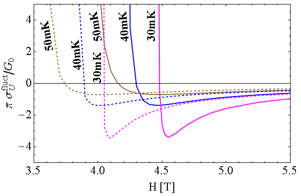
Figure 4: Normalized fluctuations conductivity, $\pi\sigma_{U}^{fluct}\left(H,T\right)/G_{0}$, as a function of field at $T=1$ mK, around its minimum, for $\beta_{0}=14$ (solid lines) and for $\beta_{0}=11$ (dashed lines), for three values of the quantum tunneling attempt rate; $T_{Q}=30$ mK (magenta), $T_{Q}=40$ mK (blue) and $T_{Q}=50$ mK (brown). Note the downward shifts of $H_{\min}$ with the decreasing values of $\beta_{0}$ and/or the increasing values of $T_{Q}$.

Realization of this scenario in 2D electron systems with strong spin-orbit scatterings under a parallel magnetic field at low temperatures shows that at sufficiently high fields the DOS conductivity prevails over the paraconductivity, resulting in strongly enhanced MR in systems with sufficiently small carriers density. Dynamical quantum tunneling of Cooper pairs, breaking into mobile normal-electrons states, contain the resistance onset at high magnetic field. In this system of heavy, charged bosons in equilibrium with unpaired mobile electrons, the dilute system of mobile electrons are responsible for most of the residual conductance.

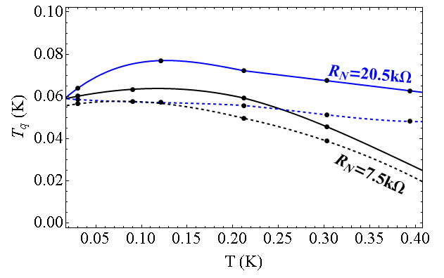
Figure 5: Best fitting values of the quantum tunneling attempt rate $T_{Q}\left(H_{\max},T\right)$ at the maximum point $H_{\max}$ of the sheet resistance as a function of Temperatures, for $\beta_{0}=11$ ($R_{N}=20.5$ k$\Omega$, blue lines), and for $\beta_{0}=14$ ($R_{N}=7.5$ k$\Omega$, black lines).  Dashed lines represent results for the fitting expression employed in Ref.MZPRB2021 , whereas the solid lines represent the results for the same expression, in which the total amplitude of $\sigma_{U}^{fluct}\left(H,T\right)$ was multiplied by 1/2.

An important feature of the localization process predicted in this approach is its dynamical nature, namely that it occurs in response to the driving electric force MZPRB2021 , and not spontaneously in a thermodynamical process toward equilibrium state. This feature seems to distinguish it from the various approaches to the phenomenon of SIT discussed in the literature Dubi07 , Bouadim2011 , GhosalPRL98 , Vinokur2008 , in which disorder-induced spatial inhomogeneity in the form of SC islands is involved in generating the insulating state. However, in a similar manner the formation of fluctuation puddles in our approach is controlled by disorder, which strongly affect the Cooper-pairs amplitude correlation function in real space. This can be seen by comparing the pair correlation function derived in the dirty limit MZPRB2021 ,CaroliMaki67I to that obtained in the pure limit CaroliMaki67II .

Another important parameter in our approach of relevance to the insulating behavior that seems to have a parallel in the literature Bouadim2011 , is the self-consistent critical shift parameter $\widetilde{\varepsilon}_{H}$, which also plays the role of an energy gap in the Cooper-pair fluctuations spectrum MZPRB2021 . Thus, it is interesting to note that the two-particle gap, which characterizes the insulating state in Ref.Bouadim2011 , vanishes at the SIT. Analogously, in our approach the (two-particle) Cooper-pair fluctuation gap $\widetilde{\varepsilon}_{H}$ gradually diminishes to very small (nonvanishing) values upon decreasing field below the sheet-resistance peak (see Fig.2 and Fig.3), in accord with the lack of a critical point.

V Acknowledgments

We would like to thank Eran Maniv, Itai Silber and Yoram Dagan for helpful discussions.

Appendix A The DOS conductivity from microscopic theory

In this appendix we evaluate the DOS conductivity in a 2D system in the zero field limit, following the fully microscopic (diagrammatic) approach presented in Ref.LV05 for a layered superconductor.

Starting with diagram No.5, and using the notation employed in Ref.LV05 (according to which $\hbar=k_{B}=1$ and the distance between layers is $s$) the corresponding response function is given by:

$$Q_{xx}^{\left(5\right)}\left(\omega\right)=i\omega\kappa_{1}\left(T\tau\right)\frac{\pi\eta_{\left(2\right)}e^{2}}{4s}A_{xx}\frac{1}{\left(2\pi\right)^{2}}\int\frac{d^{2}q}{\varepsilon+\eta_{\left(2\right)}q^{2}}$$

where $\varepsilon\equiv\ln\left(T/T_{c0}\right)$, $A_{xx}=2\left\langle v^{2}\right\rangle_{FS}/v_{F}^{2}=2\left\langle\cos^{2}\theta\right\rangle=1$, and $\eta_{\left(2\right)}=\pi D/8T$, so that by performing the integration over $x\equiv\eta_{\left(2\right)}q^{2}$, i.e.: $Q_{xx}^{\left(5\right)}\left(\omega\right)=i\omega\kappa_{1}\int_{0}^{x_{c}}dx\left(\varepsilon+x\right)^{-1}\left(e^{2}/16s\right)$, one finds:

$$Q_{xx}^{\left(5\right)}\left(\omega\right)=i\omega\kappa_{1}\frac{e^{2}}{16s}\ln\left(\frac{x_{c}}{\varepsilon}\right)$$

The corresponding conductivity:

$$\sigma_{xx}^{\left(5\right)}=-\frac{Q_{xx}^{\left(5\right)}\left(\omega\right)}{i\omega}=-\kappa_{1}\frac{e^{2}}{16s}\ln\left(\frac{x_{c}}{\varepsilon}\right)$$ (22)

which together with the topologically equivalent diagram 6 gives:

$$\sigma_{xx}^{\left(5+6\right)}=2\sigma_{xx}^{\left(5\right)}=-\kappa_{1}\frac{e^{2}}{8s}\ln\left(\frac{x_{c}}{\varepsilon}\right)$$

For the two other diagrams 7, and 8, the result is:

$$\sigma_{xx}^{\left(7+8\right)}=2\sigma_{xx}^{\left(7\right)}=-\kappa_{2}\frac{e^{2}}{8s}\ln\left(\frac{x_{c}}{\varepsilon}\right)$$

Taking into account all the four diagrams contributing to the DOS conductivity we have for the 2D limit:

$$\sigma_{xx}^{\left(5+6+7+8\right)}=-\frac{e^{2}}{8s}\kappa\left(T\tau\right)\ln\left(\frac{x_{c}}{\varepsilon}\right)$$

where:

$$\kappa\left(T\tau\right)\equiv\kappa_{1}+\kappa_{2}=\frac{-\psi^{\prime}\left(\frac{1}{2}+\frac{1}{4\pi T\tau}\right)+\frac{1}{2\pi T\tau}\psi^{\prime\prime}\left(\frac{1}{2}\right)}{\pi^{2}\left[\psi\left(\frac{1}{2}+\frac{1}{4\pi T\tau}\right)-\psi\left(\frac{1}{2}\right)-\frac{1}{4\pi T\tau}\psi^{\prime}\left(\frac{1}{2}\right)\right]}$$

Estimating $\kappa\left(T\tau\right)$ in the dirty limit: $T\tau\ll 1$ by exploiting the asymptotic expansion of the digamma function, $\psi\left(z\right)\rightarrow\ln z,\psi^{\prime}\left(z\right)\rightarrow 1/z$, we find: $\ \kappa\left(T\tau\right)_{T\tau\ll 1}\rightarrow-2\psi^{\prime\prime}\left(\frac{1}{2}\right)/\pi^{2}\psi^{\prime}\left(\frac{1}{2}\right),\psi^{\prime}\left(\frac{1}{2}\right)=\pi^{2}/2,\psi^{\prime\prime}\left(z\right)=-14\zeta\left(3\right)$, so that: $\kappa\left(T\tau\right)_{T\tau\ll 1}\rightarrow 8\times 7\zeta\left(3\right)/\pi^{4}$, and:

$$\left(\sigma_{xx}^{\left(5+6+7+8\right)}\right)_{T\tau\ll 1}\rightarrow-\kappa\left(T\tau\right)_{T\tau\ll 1}\frac{e^{2}}{8s}\ln\left(\frac{x_{c}}{\varepsilon}\right)$$ (23)

$$= -\left(\frac{7\zeta\left(3\right)}{\pi^{4}}\right)\left(\frac{e^{2}}{s}\right)\ln\left(\frac{x_{c}}{\varepsilon}\right)$$

It should be stressed at this point that this expression, which was derived here directly from the 2D limit of the response function $Q_{xx}\left(\omega\right)$, as presented in Ref.LV05 for a layered (quasi 2D) system, is by a factor of 2 larger than the 2D limit of the final expression for the total DOS conductivity reported in Ref.LV05 .

Appendix B The quantum fluctuations correction to conductivity

In this appendix we outline the physical reasoning behind our phenomenological quantum fluctuations correction to the two ingredients of the conductance fluctuations. Starting with the DOS conductivity we consider the Cooper-pair density, $n_{s}$, given in Eq.(2), with $\left\langle\left|\psi\left(q\right)\right|^{2}\right\rangle$ in Eq.(3). Approximating $7\zeta\left(3\right)\simeq 8.4$ we rewrite:

$$\left\langle\left|\psi\left(q\right)\right|^{2}\right\rangle\simeq\left(\frac{2.1E_{F}}{\pi^{2}k_{B}T}\right)\frac{1}{\Phi\left(x;\varepsilon_{H}\right)}=4.2\frac{\left(N_{2D}\lambda_{T}^{2}\right)}{\Phi\left(x;\varepsilon_{H}\right)}$$ (24)

where $N_{2D}=k_{F}^{2}/2\pi$ is the density of the 2D electron gas and $\lambda_{T}=\sqrt{\hbar^{2}/2\pi m^{\ast}k_{B}T}$ is the thermal wavelength.

The momentum distribution function $\left\langle\left|\psi\left(q\right)\right|^{2}\right\rangle$ measures the number of bosons per wave vector $\mathbf{q}$ in the Cooper-pairs liquid, engaged in equilibrium with a 2D gas of unpaired mobile electrons with a nominal density $N_{2D}$. The prefactor $N_{2D}\lambda_{T}^{2}=\left(1/2\pi^{2}\right)\left(E_{F}\tau_{T}/\hbar\right)$, that is the number of electrons in an area of size equal to the thermal wavelength, is proportional to the characteristic thermal activation time $\tau_{T}=\hbar/k_{B}T$.

The quantum corrections, introduced in Ref.MZPRB2021 , amount to modifying Expression 24 in two steps; in the first, replacing the temperature $T$, appearing in the denominator of the prefactor, with $T+T_{Q}$, and in the second step inserting the frequency-shift term $T_{Q}/2T$ to the arguments of the digamma functions in Eq.(4) consistently with the replacement of $\varepsilon_{H}$ with $\varepsilon_{H}^{U}$. The total modification takes the form:

$$\left\langle\left|\psi\left(q\right)\right|^{2}\right\rangle \rightarrow \left\langle\left|\psi_{U}\left(q\right)\right|^{2}\right\rangle=N_{2D}\lambda_{U}^{2}\frac{4.2}{\Phi_{U}\left(x;\varepsilon_{H}^{U}\right)}$$

$$= \frac{2.1}{\pi^{2}}\frac{\left(E_{F}\tau_{U}/\hbar\right)}{\Phi_{U}\left(x;\varepsilon_{H}^{U}\right)}$$

where $1/\tau_{U}=1/\tau_{T}+1/\tau_{Q}$, and $\tau_{Q}=\hbar/k_{B}T_{Q}$, is the characteristic time for Cooper-pair tunneling. The prefactor $N_{2D}\lambda_{U}^{2}$, is the number of electrons in an effective area $\lambda_{U}^{2}=\hbar^{2}/2\pi m^{\ast}k_{B}\left(T+T_{Q}\right)$ that is proportional to the characteristic time, $\tau_{U}$, for both thermal activation and quantum tunneling of Cooper pairs. Thus, increasing the temperature and/or shortening the time $\tau_{Q}$ for quantum tunneling (which also enhance pair breaking by increasing $\Phi_{U}\left(x;\varepsilon_{H}^{U}\right)$), result in larger rate of thermal and/or quantum leakage from puddles of Cooper pairs. The resulting reduction in the number of Cooper-pairs, which occurs versus a corresponding increase in the number of unpaired mobile electrons, would suppress the DOS contribution to the resistance.

The corresponding unified (quantum thermal (QT)) density (per unit area) of the Cooper-pairs liquid is now evaluated: $n_{s}^{U}=\frac{1}{d}\frac{1}{\left(2\pi\right)^{2}}\int\left\langle\left|\psi_{U}\left(q\right)\right|^{2}\right\rangle d^{2}q=\frac{1}{d}\frac{1}{\left(2\pi\right)^{2}}\int_{0}^{q_{c}^{2}}\pi d\left(q^{2}\right)\left(\frac{2.1E_{F}}{\pi^{2}k_{B}\left(T+T_{Q}\right)}\right)\frac{1}{\Phi_{U}\left(x;\varepsilon_{H}^{U}\right)}$, so that the unified DOS conductivity, $\sigma_{DOS}^{U}=-\left(2n_{s}^{U}e^{2}/m^{\ast}\right)\tau_{SO}$, is given by:

$$\sigma_{DOS}^{U}d\simeq-4.2\left(\frac{G_{0}}{\pi}\right)\int_{0}^{t^{-1}x_{0}}\frac{dx}{\left(1+T_{Q}/T\right)\Phi_{U}\left(x;\varepsilon_{H}^{U}\right)}$$ (25)

For the AL thermal fluctuations conductivity we start with the retarded current-current correlator $Q_{AL}^{R}\left(\omega\right)$, Eq.(8), which was obtained from the Matsubara correlator $Q_{AL}\left(i\Omega_{\nu}\right)$ following the analytic continuation $i\Omega_{\nu}\rightarrow\omega$.  The corresponding electrical response function is seen to be proportional to the thermal energy $k_{B}T=\hbar/\tau_{T}$.  The effects of quantum tunneling and pair breaking are introduced by adding to the thermal attempt rate $1/\tau_{T}\propto k_{B}T$ the quantum tunneling attempt rate $1/\tau_{Q}\propto k_{B}T_{Q}$ , and by appropriately inserting the frequency-shift term $T_{Q}/2T$  into the function $\Phi\left(x+\left|n+y\right|;\varepsilon_{H}\right)$, as explained in the main text, i.e.:

$$Q_{AL}^{U,R}\left(\omega\right)=k_{B}\left(T+T_{Q}\right)\left(\frac{2e}{\hbar}\right)^{2}\left(\frac{1}{2\pi d}\right)\int\limits_{0}^{x_{c}}xdx\sum\limits_{n=0,\pm 1,\pm 2,....}\frac{\Phi_{U}^{\prime}\left(x+\left|n+y\right|;\varepsilon_{H}^{U}\right)}{\Phi_{U}\left(x+\left|n+y\right|;\varepsilon_{H}^{U}\right)}\frac{\Phi_{U}^{\prime}\left(x+\left|n\right|;\varepsilon_{H}^{U}\right)}{\Phi_{U}\left(x+\left|n\right|;\varepsilon_{H}^{U}\right)}$$

where $2i\pi yk_{B}T/\hslash=\omega$.

The corresponding conductivity is: $\sigma_{AL}^{U}=\lim_{\omega\rightarrow 0}\left(i/\omega\right)\left[Q_{AL}^{U,R}\left(\omega\right)-Q_{AL}^{U,R}\left(0\right)\right]=$

$k_{B}\left(T+T_{Q}\right)\lim_{y\rightarrow 0}\left(-\frac{\hbar}{2\pi k_{B}Ty}\right)\left(\frac{2e}{\hbar}\right)^{2}\left(\frac{1}{2\pi d}\right)\int\limits_{0}^{\infty}xdx\sum\limits_{n=0,\pm 1,\pm 2,....}\left[\frac{\Phi_{U}^{\prime}\left(x+\left|n+y\right|;\varepsilon_{H}^{U}\right)}{\Phi_{U}\left(x+\left|n+y\right|;\varepsilon_{H}^{U}\right)}\frac{\Phi_{U}^{\prime}\left(x+\left|n\right|;\varepsilon_{H}^{U}\right)}{\Phi_{U}\left(x+\left|n\right|;\varepsilon_{H}^{U}\right)}-\frac{\Phi_{U}^{\prime}\left(x+\left|n\right|;\varepsilon_{H}^{U}\right)}{\Phi_{U}\left(x+\left|n\right|;\varepsilon_{H}^{U}\right)}\frac{\Phi_{U}^{\prime}\left(x+\left|n\right|;\varepsilon_{H}^{U}\right)}{\Phi_{U}\left(x+\left|n\right|;\varepsilon_{H}^{U}\right)}\right]$

$=-\left(\frac{T+T_{Q}}{T}\right)\left(\frac{e}{\pi}\right)^{2}\left(\frac{1}{d\hbar}\right)\int\limits_{0}^{\infty}xdx\sum\limits_{n=0,\pm 1,\pm 2,....}\frac{\Phi_{U}^{\prime}\left(x+\left|n\right|;\varepsilon_{H}^{U}\right)}{\Phi_{U}\left(x+\left|n\right|;\varepsilon_{H}^{U}\right)}\lim_{y\rightarrow 0}\frac{1}{y}\left[\frac{\Phi_{U}^{\prime}\left(x+\left|n+y\right|;\varepsilon_{H}^{U}\right)}{\Phi_{U}\left(x+\left|n+y\right|;\varepsilon_{H}^{U}\right)}-\frac{\Phi_{U}^{\prime}\left(x+\left|n\right|;\varepsilon_{H}^{U}\right)}{\Phi_{U}\left(x+\left|n\right|;\varepsilon_{H}^{U}\right)}\right]$,  which can be reduced to (compare Eq.9):

$$\sigma_{AL}^{U}d=\frac{1}{4}\left(\frac{G_{0}}{\pi}\right)\left(1+\frac{T_{Q}}{T}\right)\int\limits_{0}^{t^{-1}x_{0}}\left(\frac{\Phi_{U}^{\prime}\left(x;\varepsilon_{H}^{U}\right)}{\Phi_{U}\left(x;\varepsilon_{H}^{U}\right)}\right)^{2}dx$$ (26)

$R_{N}=7.5[k\Omega$]						$R_{N}=10.5[k\Omega$]						$R_{N}=20.5[k\Omega$]
$T[mK]$	$T_{q}[mK]$	$H_{q}[T]$	$H_{n}[T]$	$\sigma_{0}[k\Omega^{-1}]$		$T[mK]$	$T_{q}[mK]$	$H_{q}[T]$	$H_{n}[T]$	$\sigma_{0}[k\Omega^{-1}]$		$T[mK]$	$T_{q}[mK]$	$H_{q}[T]$	$H_{n}[T]$	$\sigma_{0}[k\Omega^{-1}]$
30	83	8	6.9	.065		30	80	7.3	7	.041		30	97	6.5	4.25	.014
90	77	10	7	.065		130	75	10	7.1	.041		121	90	10	4.35	.014
212	62	20	12	.09		230	62	15	8	.051		212	82	10	4.5	.015
303	47	25	14	.096		330	55	18	10	.065		303	72	12	6.5	.026
485	10	30	20	.106		430	35	25	12	.069		394	67	15	8	.029

Table 1: Values of the temperature-dependent parameters extracted in the fitting process of the measured sheet resistance for the 1/2-reduced amplitude of $\sigma^{fluct}\left(H,T\right)$, which determine the temperature and field dependencies of the phenomenological parameters $\sigma_{n}\left(H,T\right)$ and $T_{Q}\left(T,H\right)$ (see Appendix D for details).  As elaborated in Ref. MZPRB2021 , the three gate voltages employed correspond to $R_{N}=20.5,10.5,7.5$ k$\Omega$ .

Appendix C The Quantum limit of the Critical-shift parameter

In this appendix we study the pair-breaking effect due to magnetic field and to quantum tunneling of Cooper pairs in the zero temperature limit.  Consider the unified (quantum-thermal) expression, Eq.(II), for the critical shift parameter $\varepsilon_{h}^{U}$ in the zero-temperature (quantum) limit.

Using the asymptotic expansion of $\psi\left(\frac{1}{2}+T_{Q}/2T+f_{\pm}\right)$ for $T_{Q}/T,$ $f_{\pm}\gg 1$, i.e. $\psi\left(\frac{1}{2}+T_{Q}/2T+f_{\pm}\right)\rightarrow\ln\left(T_{Q}/2T+f_{\pm}\right)=\ln\left[\left(T_{Q}+T_{\pm}\right)/2T\right]$, we have:

$$\varepsilon_{h}^{U}\rightarrow\varepsilon_{h}^{Q}=\ln\left(T/T_{c0}\right)-\ln T+$$ (27)

$$a_{+}\ln\left(T_{Q}+T_{-}\right)+a_{-}\ln\left(T_{Q}+T_{+}\right)-\ln 2-\psi\left(1/2\right)$$

where:

$$T_{\pm}\equiv\frac{D\left(de\right)^{2}H^{2}}{\pi k_{B}\hslash}+\frac{\varepsilon_{SO}}{2\pi k_{B}}\pm\sqrt{\left(\frac{\varepsilon_{SO}}{2\pi k_{B}}\right)^{2}-\left(\frac{\mu_{B}H}{\pi k_{B}}\right)^{2}}$$ (28)

In the above expression for $\varepsilon_{h}^{Q}$ (Eq.27), the Cooper singular term, $\ln\left(T/T_{c0}\right)$, is exactly cancelled by the logarithmic term arising from the asymptotic expansion of the digamma functions, so that the remaining regular terms are rearranged to yield the following temperature independent expression for ${\normalsize\varepsilon_{h}^{Q}}$:

$${\normalsize\varepsilon_{h}^{Q}\rightarrow a_{+}\ln\left(\frac{T_{Q}+T_{-}}{T_{c0}}\right)+a_{-}\ln\left(\frac{T_{Q}+T_{+}}{T_{c0}}\right)+\ln 2+\gamma}$$ (29)

where $\gamma\approx 0.5772$… is the Euler–Mascheroni constant, and:

$$a_{\pm}=\frac{1}{2}\left(1\pm\frac{1}{\sqrt{1-\left(\mu_{0}/\beta_{0}\right)^{2}h^{2}}}\right)$$

with $\mu_{0}\equiv\mu_{B}H_{c\parallel 0}^{\ast}/2\pi k_{B}T_{c}^{\ast},\beta_{0}\equiv\varepsilon_{SO}/4\pi k_{B}T_{c}^{\ast}$.

Appendix D The phenomenological fitting parameters

As in our fitting process, described in Ref.MZPRB2021 , the normal-state conductivity contribution $\sigma_{n}\left(H,T\right)$ has a quadratic field-dependent form: $\sigma_{n}\left(H,T\right)=\sigma_{0}\left(T\right)\left[1+\left(H/H_{n}\left(T\right)\right)\right]^{2}$, with two adjustable, temperature-dependent parameters $\sigma_{0}\left(T\right),H_{n}\left(T\right)$. The corresponding expression for the MR, defined as usual by: $MR\left(H,T\right)\equiv\left[\rho_{n}\left(H,T\right)-\rho_{n}\left(0,T\right)\right]/\rho_{n}\left(0,T\right)$, where $\rho_{n}\left(H,T\right)=1/\sigma_{n}\left(H,T\right)$, is given by:

$$MR\left(H,T\right)=-\frac{\left(H/H_{n}\left(T\right)\right)^{2}}{1+\left(H/H_{n}\left(T\right)\right)^{2}}$$ (30)

yielding negative MR in qualitative agreement with that observed in Refs.RoutPRB17 and DiezPRL15  at temperatures well above $T_{c}$.

Similarly, for the temperature and field dependence of the phenomenological quantum tunneling "temperature" parameter $T_{Q}\left(T,H\right)$ we use here the form employed in Ref.MZPRB2021 :

$$T_{Q}\left(T,H\right)=T_{Q}\left(T\right)\left[1-\left(\frac{H}{H_{Q}\left(T\right)}\right)^{2}\right]$$ (31)

with the two adjustable parameters, $T_{Q}\left(T\right)$ and $H_{Q}\left(T\right)$.

The best fitting values for $T_{Q}\left(T\right),H_{Q}\left(T\right),H_{n}\left(T\right)$, and $\sigma_{0}\left(T\right)$, obtained in our fitting process for the 1/2-reduced amplitude of $\sigma^{fluct}\left(H,T\right)$ are listed in Table I.

References

- (1) T. Maniv and V. Zhuravlev, "Superconducting fluctuations and giant negative magnetoresistance in a gate-voltage tuned two-dimensional electron system with strong spin-orbit impurity scattering", Phys. Rev. B 104, 054503 (2021).
- (2) A. Ohtomo, and H. Y. Hwang, "A high-mobility electron gas at the LaAlO3/SrTiO3 heterointerface", Nature 427, 423 (2004).
- (3) M. Mograbi, E. Maniv, P. K. Rout, D. Graf, J. -H Park and Y. Dagan, "Vortex excitations in the Insulating State of an Oxide Interface", Phys. Rev. B 99, 094507 (2019).
- (4) S. Ullah and A.T. Dorsey, "Critical Fluctuations in High-Temperature Superconductors and the Ettingshausen Effect", Phys. Rev. Lett. 65, 2066 (1990). Properties of (111) LaAlO3/SrTiO3", Phys. Re. Lett. 123, 036805 (2019).
- (5) S. Ullah and A.T. Dorsey, "Effect of fluctuations on the transport properties of type-II superconductors in a magnetic field", Phys. Rev. B 44, 262 (1991).
- (6) L. G. Aslamazov and A.I. Larkin, Phys. Lett. A 26 p. 238 (1968).
- (7) A. Larkin and A. Varlamov, "Theory of fluctuations in superconductors", Oxford University Press 2005.
- (8) In Ref.MZPRB2021 we have made two technical errors, which nearly cancelled each other, while approximately arriving to the exact expression 23 derived in Appendix A.
- (9) Estimation of the argument of the logarithmic factor in Eq.(15) just above the "nominal" critical field T () in the limit, based on typical values of our fitting parameters yields . Estimations of the field-dependent prefactors of the AL and the DOS conductivities under the same conditions yield, respectively: .
- (10) N. Shah and A. V. Lopatin, "Microscopic analysis of the superconducting quantum critical point: Finite-temperature crossovers in transport near a pair-breaking quantum phase transition", Phys. Rev. B 76, 094511 (2007).
- (11) A. V. Lopatin, N. Shah, and V. M. Vinokur, "Fluctuation Conductivity of Thin Films and Nanowires Near a Parallel-Field-Tuned Superconducting Quantum Phase Transition", Phys. Rev. Lett. 94, 037003 (2005).
- (12) A. D. Caviglia, S. Gariglio, N. Reyren, D. Jaccard, T. Schneider, M. Gabay, S. Thiel, G. Hammerl, J. Mannhart and J.-M. Triscone, "Electric field control of the LaAlO3/SrTiO3 interface ground state", Nature (London) 456, 624 (2008).
- (13) J. Biscaras, N. Bergeal, S. Hurand, C. Feuillet-Palma, A. Rastogi, R. C. Budhani, M. Grilli, S. Caprara and J. Lesueur, "Multiple quantum criticality in a two-dimensional superconductor", Nat. Mater. 12, 542 (2013).
- (14) M. M. Mehta, D. A. Dikin, C. W. Bark, S. Ryu, C. M. Folkman, C. B. Eom, and V. Chandrasekhar, "Magnetic field tuned superconductor-to-insulator transition at the LaAlO3/SrTiO3 interface", Phys. Rev. B 90, 100506 (2014).
- (15) M. Diez, A. M. R. V. L. Monteiro, G. Mattoni, E. Cobanera, T. Hyart, E. Mulazimoglu, N. Bovenzi, C.W. J. Beenakker, and A. D. Caviglia, "Giant Negative Magnetoresistance Driven by Spin-Orbit Coupling at the LaAlO3/SrTiO3 Interface", Phys. Re. Lett. 115, 016803 (2015).
- (16) Udit Khanna, P. K. Rout, Michael Mograbi, Gal Tuvia, Inge Leermakers, Uli Zeitler, Yoram Dagan, and Moshe Goldstein, "Symmetry and Correlation Effects on Band Structure Explain the Anomalous Transport Properties of (111) LaAlO3/SrTiO3", Phys. Re. Lett. 123, 036805 (2019).
- (17) Arjun Joshua, S. Pecker, J. Ruhman, E. Altman and S. Ilani, "A universal critical density underlying the physics of electrons at the LaAlO3/SrTiO3 interface", Nat. Commun. 3, 1129 (2012).
- (18) Y. Dubi, Y. Meir and Y. Avishai, "Nature of the superconductor–insulator transition in disordered superconductors", Nature 449, 876 (2007).
- (19) K. Bouadim, Y. L. Loh, M. Randeria and N. Trivedi, "Single- and two-particle energy gaps across the disorder-driven superconductor–insulator transition", Nature Phys. 7, 884 (2011).
- (20) A. Ghosal, M. Randeria, and N. Trivedi, "Role of Spatial Amplitude Fluctuations in Highly Disordered s-Wave Superconductors", Phys. Re. Lett. 81, 3940 (1998).
- (21) V. Vinokur, T. I. Baturina, M. V. Fistul, A. Yu. Mironov, M. R. Baklanov and C. Strunk, "Superinsulator and quantum synchronization", Nature 452, 613 (2008).
- (22) C. Caroli and K. Maki, "Fluctuations of the Qrder Parameter in Type-II Superconductors. I. Dirty Limit", Phys. Rev. 159, 306 (1967).
- (23) C. Caroli and K. Maki, "Fluctuations of the Qrder Parameter in Type-II Superconductors. II. Pure Limit", Phys. Rev. 159, 316 (1967).
- (24) P. K. Rout, I. Agireen, E. Maniv, M. Goldstein, and Y. Dagan, "Six-fold crystalline anisotropic magnetoresistance in the (111) LaAlO3/SrTiO3 oxide interface", Phys. Rev. B 95, 241107(R) (2017).