Compressed Training for Dual-Wideband Time-Varying Sub-Terahertz Massive MIMO

Abstract

6G operators may use millimeter wave (mmWave) and sub-terahertz (sub-THz) bands to meet the ever-increasing demand for wireless access. Sub-THz communication comes with many existing challenges of mmWave communication and adds new challenges associated with the wider bandwidths, more antennas, and harsher propagations. Notably, the frequency- and spatial-wideband (dual-wideband) effects are significant at sub-THz. This paper presents a compressed training framework to estimate the time-varying sub-THz MIMO-OFDM channels. A set of frequency-dependent array response matrices are constructed, enabling channel recovery from multiple observations across subcarriers via multiple measurement vectors (MMV). Using the temporal correlation, MMV least squares (LS) is designed to estimate the channel based on the previous beam support, and MMV compressed sensing (CS) is applied to the residual signal. We refer to this as the MMV-LS-CS framework. Two-stage (TS) and MMV FISTA-based (M-FISTA) algorithms are proposed for the MMV-LS-CS framework. Leveraging the spreading loss structure, a channel refinement algorithm is proposed to estimate the path coefficients and time delays of the dominant paths. To reduce the computational complexity and enhance the beam resolution, a sequential search method using hierarchical codebooks is developed. Numerical results demonstrate the improved channel estimation accuracy of MMV-LS-CS over state-of-the-art techniques.

I Introduction

Future wireless applications will require networks to provide high rates, reduced power consumption, and low latency in a wide range of deployment scenarios [2]. These requirements motivate policy and technical research on making spectrum at higher frequencies, outside the popularly used sub-6 GHz spectrum, commercially available for wireless broadband thanks to large bandwidth availability. In 5G, this technical work culminated in the standardization and deployment of communications in the millimeter wave (mmWave) spectrum.

In the sub-terahertz (sub-THz) spectrum, roughly defined as $100-300$ GHz, there is approximately $21.2$ GHz available for wireless broadband [3]. Making these bands “usable” promises to alleviate backhaul and access concerns far into the future [3, 4, 5]. Unfortunately, sub-THz communication poses signal processing and wideband communication challenges unique to the spectrum. Notable challenges include the need for i) a dramatic increase in bandwidth and antenna aperture and ii) signal processing techniques that leverage the unique propagation features. As dictated by Friis’ equation, the spreading loss increases with the operating frequency, inducing a more serious issue in sub-THz than in mmWave or sub-6 GHz systems [6]. Caused mainly by water vapor, molecular absorption loss becomes more pronounced as the frequency increases [7]. Also, the reflection coefficient [8] should be considered when modeling the pathloss of the sub-THz channel in non-line-of-sight (NLOS). By combining these effects together, the overall pathloss is a frequency-selective attenuation. To compensate for such severe signal attenuation, sub-THz systems require highly-directional beamforming via massive multiple-input multiple-output (MIMO) [9]. Thanks to the short wavelength of sub-THz signals, massive MIMO is possible even with a small form factor. However, the hardware limitations (e.g., high power consumption and cost) of the radio frequency (RF) chains in massive MIMO make digital baseband precoding infeasible. An analog precoder overcomes the hardware limitation but suffers from performance degradation. To achieve larger precoding gains with a limited number of RF chains, hybrid transceiver structures have been proposed and investigated in [10, 11]. Our work focuses on the design of a channel training algorithm under a hybrid transceiver structure.

Orders-of-Magnitude Larger Bandwidths and Wideband Effects: Frequency-wideband and spatial-wideband effects of the MIMO channel will be exacerbated in sub-THz systems. The frequency-wideband effect is caused by the delay spread of the multipath channel responses. The spatial-wideband effect arises from differences in time delays across the antenna aperture. This primarily arises because the angles of arrival of the propagation paths observed by the receiver vary within the operating frequencies, known as the beam squint effect [12, 13, 14, 15, 11, 16]. Most existing works focusing on sub-6 GHz or mmWave systems [10, 17, 18, 19, 20, 21, 22, 23, 24, 25] consider only the frequency-wideband effect but ignore the spatial-wideband effect since it is negligible when the available bandwidth is not very wide, which is a reasonable assumption in current and past wireless deployments. However, sub-THz communication systems may use one order of magnitude more bandwidth than mmWave communication systems [3], hence are more severely affected by the wideband effect. Motivated by this fact, in this paper, we are concerned with both effects, meaning that we consider systems with dual-wideband (also known as spatial-frequency wideband) effects. To this end, we develop an accurate channel model capturing the dual-wideband effect for sub-THz communication systems.

Because of the promising beamforming gains, massive MIMO communication systems with dual-wideband effects are employed to compensate for the impairments of sub-THz channels. MIMO orthogonal frequency division multiplexing (MIMO-OFDM) has been envisioned as a vital tool to combat the frequency-wideband effect and inter-symbol interference of the multipath channel. For MIMO-OFDM channel estimation, the works [21, 22] recover the channel from multiple measurements among subcarriers sharing a common support, known as multiple measurement vectors (MMV). Yet, the works [21, 22] neglect the spatial-wideband effect, which breaks the common support assumption across subcarriers and degrades the estimation accuracy. The work [11] addresses the issue by designing a set of frequency-dependent dictionary matrices to preserve the common support across subcarriers, mitigating the estimation losses from the spatial-wideband effect. However, the work [11] does not exploit the temporal correlation in the time-varying MIMO-OFDM systems to aid the channel training, which is the focus of this paper.

Few dominant paths and channel sparsity: Massive MIMO requires accurate channel state information (CSI) acquired via channel estimation to enable coherent alignment in narrow beam communications for high beamforming gains. Yet, traditional MIMO channel estimation techniques are impractical due to the prohibitive overhead that comes with (non-adaptive) omni-directional training over a large number of antennas. This burden can be reduced by exploiting the fact that the MIMO channel in sub-THz bands is determined by the geometry (positions and antenna geometry) of the transmitter and receiver, and exhibits a high degree of channel sparsity, with few propagation clusters. For instance, the work [26] reported an average of 6 clusters and 4 multipath components (MPCs) per cluster at 140GHz, compared to 8 clusters and 5 MPCs per cluster at 28GHz. One approach is to utilize a predetermined set of beams (e.g., a codebook), usually designed to allocate power in specific directions, and to tailor the channel training algorithm to this lower-dimensional beam set instead of the true higher-dimensional MIMO channel. For example, the most-discussed approach [27, 28] is to scan over some set of candidate beams and estimate the strongest (e.g., through received power measurement), but even this approach incurs a prohibitively large overhead due to the typically large size of the beamforming codebook. This issue is exacerbated in time-varying channels, due to the need for periodic beam training. For time-varying channels, one approach is to model the dynamic behavior of the channel as a birth-death process of MPCs [29, 30], which models the temporal correlation of the surviving MPCs. The channel sparsity, combined with the slow temporal variations, results in slowly-varying beam support, which could be exploited for MIMO channel estimation [31]. Channel estimation algorithms exploiting the temporal correlation of the channel, via the use of a common (or slow-varying) channel support over time, have been studied for narrowband MIMO systems in [31] and for frequency-wideband multiuser MIMO-OFDM systems in [21]. Nevertheless, these techniques cannot be directly applied to time-varying dual-wideband MIMO-OFDM channels due to the beam squint effect and frequency-dependent path gains, which may harm the estimation performance. To address the issues, we propose a new channel training framework (MMV-LS-CS) in time-varying dual-wideband MIMO-OFDM systems with a hybrid transceiver structure and a channel refinement algorithm that leverages the spreading loss structure to improve the estimation performance by deriving the path coefficients and time delays of the dominant paths across the pilot subcarriers.

Prior Works

Over the last decade, researchers have focused on MIMO channel estimation in mmWave and (sub-)THz bands. Several works focused on the beam alignment problem, including feedback-based schemes [32, 33, 34, 35, 36, 37, 38, 39, 40], data-assisted schemes [41, 42, 43, 44], and multipath estimation [10, 17, 31, 18, 19, 20, 21, 22, 23, 24, 25, 12, 13, 11, 14, 15]. Feedback-based schemes adapt the beam training according to the feedback information sent from the receiver in an online fashion [32] or leverage the UEs’ mobility as in [33, 34]. Data-assisted schemes perform the beam training by using side information from other available sources, e.g., GPS positional information [41], lower-frequency communication [42], radar [43], and LIDAR [44]. Multipath estimation schemes can exploit the channel sparsity of the MIMO channel via compressed sensing (CS) to acquire the associated channel parameters, e.g., angles of arrival (AOAs), angles of departure (AODs), time delays, and path gains. The channel training proposed in this work is a form of multipath estimation.

The narrowband MIMO channel estimation problem has been investigated in [10, 17]. The work [10] proposes an adaptive algorithm for mmWave massive MIMO channel estimation using a hierarchical multi-resolution codebook. With an adaptive structure, the work [17] proposes channel estimation using a compressive beacon codebook with different pseudorandom phase settings of the antenna arrays. In contrast to [10, 17], our work focuses on wideband MIMO channel estimation, taking advantage of the abundant bandwidth available in sub-THz bands.

Initial works on wideband MIMO channel estimation considering the frequency-wideband include [18, 19, 20, 21, 22, 23, 24, 25]. Assuming channel sparsity, the work [18] formulates MIMO-OFDM channel estimation as a sparse recovery problem solved via orthogonal matching pursuit (OMP). The work [19] applies a tensor decomposition to the training signal with multiple dimensions corresponding to the beams and subcarriers and proposes a CANDECOMP/PARAFAC decomposition-based algorithm. The work [20] proposes a CS-aided channel estimation using the Tucker tensor as a compressible representation and reconstruction by tensor-OMP (T-OMP). These works, however, do not leverage the dual-wideband structure of wideband MIMO-OFDM channels.

Dual-wideband estimation of MIMO-OFDM channels has been studied in [12, 13, 14, 15, 11, 16]. The challenges of dual-wideband MIMO in mmWave are outlined in [12], and a channel estimation strategy exploiting the asymptotic characteristics of the channel is proposed. The work [13] presents a CS-aided channel estimation on dual-wideband MIMO-OFDM exploiting uplink/downlink channel reciprocity. The work in [14] considers the block sparsity of the beam squint effect to design a CS-based channel estimation. A tensor-based channel training using the Vandermonde constraint and spatial smoothing method is proposed in [15]. The dual-wideband effect in THz communications with uniform planar arrays (UPAs) is studied in [11], and an algorithm (GSOMP) to recover the channel by simultaneous OMP exploiting the common support across the subcarriers preserved by the frequency-dependent dictionary matrices is proposed (evaluated numerically in Section V). These prior works, however, do not address channel estimation over time-varying channels. In fact, the channel tends to manifest temporal correlation between consecutive frames, which may be leveraged to improve channel estimation. In our work, we devise a channel training framework in dual-wideband MIMO-OFDM that uses the temporal correlation and common support across the frequencies to improve the estimation performance.

Contributions

We develop a support tracking-based channel training framework utilizing the estimated previous channel support for time-varying sub-THz dual-wideband MIMO-OFDM systems. For the spatial-wideband effect, a set of frequency-dependent array response matrices are constructed to preserve the common channel support, leading to the MMV formulation of recovering the sparse beamspace channel from multiple observations across subcarriers. In a slowly-varying channel, the channel supports of consecutive frames tend to share many common elements, enabling the LS-CS residual approach [45, 46], that substitutes the CS on the measurements with the CS on the LS residual signal. We propose channel estimation that incorporates the MMV and LS-CS residual approach, called two-stage MMV-LS-CS (TS). In addition, we formulate a joint MMV-LS-CS optimization problem, and solve it using the framework of the Fast Iterative Shrinkage-Thresholding Algorithm (FISTA) [47], called MMV FISTA (M-FISTA).

In summary, the contributions of this paper are as follows:

• We propose a support tracking-based channel training framework, MMV-LS-CS, for time-varying dual-wideband MIMO-OFDM systems with hybrid transceivers using the estimated previous channel support.

• We propose two channel estimation algorithms in MMV-LS-CS framework: TS and M-FISTA.

  • The TS algorithm does MMV-LS estimation on the estimated previous channel support, followed by MMV-CS estimation on the residual to estimate the time-varying channel components. Note that TS can reduce its average execution time by parallel processing. However, inaccurate estimated previous channel support might induce the channel estimation error in MMV-LS, and an increased number of channel elements is expected to be estimated in MMV-CS.

  • To avoid the issue, the M-FISTA algorithm uses the framework of FISTA to solve a joint version of MMV-LS-CS optimization problem for the channel estimation. Unlike TS, M-FISTA is more resilient to the inaccuracy in the previous estimated channel. However, M-FISTA can not operate with parallel processing to reduce the average execution time.

  • Numerical results show that M-FISTA achieves a more accurate channel estimation than TS. Nonetheless, TS with parallel processing requires only $32$% of the average execution time of M-FISTA. It shows the trade-off of estimation accuracy and computational complexity between these two algorithms.

• We propose two additional operations, channel refinement and sequential search, to enhance the channel estimation performance. The channel refinement leverages the spreading loss structure to derive the path gains and time delays of the estimated paths across the subcarriers, so the channel on all subcarriers can be reconstructed from the training measurements on the pilot subcarriers. The sequential search uses the hierarchical codebooks to reduce the computational complexity of the greedy beam selection in TS and increase the beam resolution in M-FISTA.

The rest of the paper is organized as follows. Section II introduces the channel and signal model. Section III proposes two channel estimation algorithms (TS and M-FISTA) in MMV-LS-CS training framework. Section IV develops the operations (channel refinement and sequential search) to enhance the performance, followed by the complexity analyses. Section V shows the numerical results, and Section VI concludes the paper.

Notation: Bold lowercase letters $\mathbf{x}$ and bold uppercase letters $\mathbf{X}$ denote vectors and matrices, respectively; $\mathbf{X}^{\top}$, $\mathbf{X}^{H}$, $\mathbf{X}^{+}$, $\textrm{vec}(\mathbf{X})$, $\textrm{det}(\mathbf{X})$ represent the transpose, conjugate transpose, Moore-Penrose pseudo-inverse, vectorization, and determinant of $\mathbf{X}$, respectively; $[\mathbf{X}]_{\Gamma}$ (respectively, $[\mathbf{x}]_{\Gamma}$) is the submatrix with columns of $\mathbf{X}$ (the subvector with elements of $\mathbf{x}$) associated with the indices set $\Gamma$; $(\mathbf{X})_{\mathbf{n}}$ is the $\mathbf{n}$-th element of $\mathbf{X}$; $\lvert\Psi\rvert$ is the cardinality of the set $\Psi$; $\otimes$ denotes the Kronecker product; $\mathbf{I}_{M}$ is an $M\times M$ identity matrix; $\mathcal{F}\{\cdot\}$ is the continuous Fourier transform. $\textrm{bdiag}(\mathbf{X}_{1},\dots,\mathbf{X}_{N})$ is a block diagonal matrix having the matrices $\mathbf{X}_{1},\dots,\mathbf{X}_{N}$ on its diagonal.

II System Model

Clearly defining the system model in sub-THz is critical. Section II-A describes a time-varying sub-THz wideband channel model. Section II-B discusses its frequency selectivity. Section II-C introduces the signal model of the hybrid transceiver, and Section II-D describes the extended virtual representation of the MIMO channel.

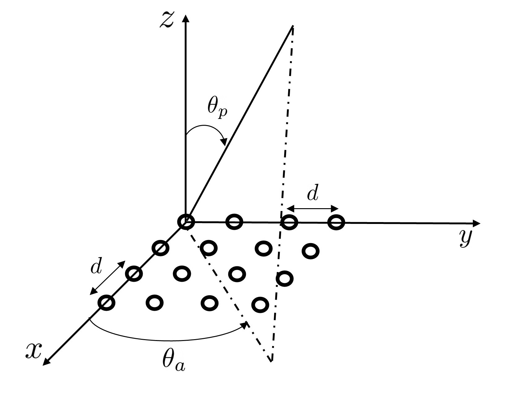
Figure 1: The array geometry of a $4\times 4$ UPA with the physical angle $(\theta_{p},\theta_{a})$ [48].

II-A Channel Model

We consider a MIMO-OFDM system with bandwidth $B$, carrier frequency $f_{c}$, and $K_{o}$ subcarriers. We define $\Delta\in[-B/2,B/2]$ as the baseband frequency centered at the carrier frequency $f_{c}$ so that the actual frequency is $f=f_{c}+\Delta$. Since $f_{c}$ is fixed, the dependence of the channel propagation quantities (such as attenuation, etc) on the carrier frequency $f_{c}$ is not shown explicitly. The receiver and transmitter employ a UPA with $N_{r}\!=\!N_{vr}\!\times\!N_{hr}$ antennas and a UPA with $N_{t}\!=\!N_{vt}\!\times\!N_{ht}$ antennas, respectively, both configured with antenna spacing $d$, as depicted in Fig. 1. The receive and transmit antennas are indexed as $\mathbf{n}_{r}=(n_{vr},n_{hr})$ and $\mathbf{n}_{t}=(n_{vt},n_{ht})$, respectively. We adopt a wideband geometric massive MIMO channel model with $L$ channel paths between the transmitter and receiver [49]. The $\ell$-th channel path ($\ell\!=\!1,\dots,L$) is characterized by its frequency-selective attenuation $\mathcal{B}_{\ell}(\Delta)$, time delay $\tau_{\ell}$, physical AOA $\boldsymbol{\theta}_{r}^{\ell}\!=\!(\theta_{pr}^{\ell},\theta_{ar}^{\ell})$, and physical AOD $\boldsymbol{\theta}_{t}^{\ell}\!=\!(\theta_{pt}^{\ell},\theta_{at}^{\ell})$, specifying the polar and azimuth angles (indexed by “$\mathit{p}$” and “$\mathit{a}$”, respectively). The time-domain response of the $\ell$-th channel path is denoted as $\beta_{\ell}(t;u)$. With the slowly-varying channel, the channel parameters are unchanged within the channel coherence time, so we omit the time variable $u$ of the channel parameters for ease of exposition. Due to the frequency selectivity of the interactions with the environment [50], $\beta_{\ell}(t)$ models the distortion of the $\ell$-th channel path with $\mathcal{F}\{\beta_{\ell}(t)\}=\mathcal{B}_{\ell}(\Delta)$, where $\mathcal{B}_{\ell}(\Delta)$ is the frequency-selective attenuation introduced in Section II-B. The baseband signal at the $\mathbf{n}_{r}$-th receive antenna is

$$r_{\mathbf{n}_{r}}(u)=\sum_{\mathbf{n}_{t}}\sum_{\ell=1}^{L}{\tilde{x}}_{{\ell},\mathbf{n}_{t}}(u-\tau_{\ell,\mathbf{n}_{r},\mathbf{n}_{t}})e^{-j2\pi f_{c}\tau_{\ell,\mathbf{n}_{r},\mathbf{n}_{t}}}+v_{\mathbf{n}_{r}}(u),$$ (1)

where $\tau_{\ell,\mathbf{n}_{r},\mathbf{n}_{t}}$ is the time delay of the $\ell$-th channel path between the $\mathbf{n}_{t}$-th transmit antenna and $\mathbf{n}_{r}\textrm{-th}$ receive antenna, $v_{\mathbf{n}_{r}}(u)$ is the additive noise at the $\mathbf{n}_{r}$-th receive antenna, and $\tilde{x}_{{\ell},\mathbf{n}_{t}}(u)\!=\!\beta_{\ell}\ast{x}_{\mathbf{n}_{t}}(u)$ is the convolution of the baseband signal ${x}_{\mathbf{n}_{t}}(u)$ transmitted at the $\mathbf{n}_{t}$-th antenna with the frequency-selective attenuation of the $\ell$-th channel path $\beta_{\ell}(t)$. Note that $\beta_{\ell}(t)$ is assumed the same for the $\ell$-th channel path between all possible pairs of the transmit and receive antennas, due to the fact that path gains are large-scale fading channel components.

Due to the increasing scale of the antenna arrays, the time delay of waves traveling across the array aperture is non-negligible, so we denote the time delay as [51]

$$\tau_{\ell,\mathbf{n}_{r},\mathbf{n}_{t}}=\tau_{\ell}+\tau_{\mathbf{n}_{r}}(\boldsymbol{\theta}_{r}^{\ell})-\tau_{\mathbf{n}_{t}}(\boldsymbol{\theta}_{t}^{\ell}),$$ (2)

where $\tau_{\ell}$ is the reference path delay of the $\ell$-th channel path on the first transmit and receive antenna pair ($\mathbf{n}_{t}\!=\!\mathbf{n}_{r}\!=\!(1,1)$). The propagation delay of the $\mathbf{n}_{r}$-th receive ($\mathbf{n}_{t}$-th transmit) antenna across the UPA aperture with respect to the $(1,1)$-th receive (transmit) antenna is denoted as $\tau_{\mathbf{n}_{\zeta}}(\boldsymbol{\theta}_{\zeta}^{\ell})\!=\!\frac{d}{c}\Big{(}(n_{h\zeta}-1)\cos\theta_{a\zeta}^{\ell}\sin\theta_{p\zeta}^{\ell}+(n_{v\zeta}-1)\sin\theta_{a\zeta}^{\ell}\sin\theta_{p\zeta}^{\ell}\Big{)},$ $\zeta\!\in\!\{r,t\}$ [48]. By applying the continuous Fourier transform on (1), we obtain the signal at the baseband frequency $\Delta$ as

$$(\mathbf{R}(\Delta))_{\mathbf{n}_{r}}=\mathcal{F}\{r_{\mathbf{n}_{r}}(u)\}=$$

$$\sum_{\mathbf{n}_{t}}\sum_{\ell=1}^{L}\alpha_{\ell}(\Delta)e^{-j2\pi(f_{c}+\Delta)\left(\tau_{\mathbf{n}_{r}}(\boldsymbol{\theta}_{r}^{\ell})-\tau_{\mathbf{n}_{t}}(\boldsymbol{\theta}_{t}^{\ell})\right)}e^{-j2\pi\Delta\tau_{\ell}}(\mathbf{X}(\Delta))_{\mathbf{n}_{t}}$$

$$+(\mathbf{V}(\Delta))_{\mathbf{n}_{r}},$$

where $(\mathbf{X}(\Delta))_{\mathbf{n}_{t}}\!\!=\!\mathcal{F}\{{x}_{\mathbf{n}_{t}}(u)\}$, $(\mathbf{V}(\Delta))_{\mathbf{n}_{r}}\!\!=\!\mathcal{F}\{v_{\mathbf{n}_{r}}(u)\}$, and we define the baseband path coefficient

$$\alpha_{\ell}(\Delta)\triangleq\mathcal{B}_{\ell}(\Delta)e^{-j2\pi f_{c}\tau_{\ell}}.$$ (3)

By stacking up the MIMO signal on UPA antennas, we obtain the frequency-dependent input-output relationship for the MIMO channel as

$$\mathbf{r}(\Delta)=\mathbf{H}(\Delta)\mathbf{x}(\Delta)+\mathbf{v}(\Delta),$$ (4)

where $\mathbf{r}(\Delta)=\textrm{vec}(\mathbf{R}(\Delta))\in\mathbb{C}^{N_{r}\times 1}$ is the received signal vector, $\mathbf{x}(\Delta)=\textrm{vec}(\mathbf{X}(\Delta))\in\mathbb{C}^{N_{t}\times 1}$ is the transmit signal vector, and ${\mathbf{v}(\Delta)=\textrm{vec}(\mathbf{V}(\Delta))\in\mathbb{C}^{N_{r}\times 1}}$ is the additive noise vector. The frequency response of the baseband MIMO channel $\mathbf{H}(\Delta)\in\mathbb{C}^{N_{r}\times N_{t}}$ is

$$\mathbf{H}(\Delta)=\sqrt{N_{r}N_{t}}\times$$

$$\sum_{\ell=1}^{L}\alpha_{\ell}(\Delta)\mathbf{b}_{N_{r}}(\psi_{hr}^{\ell},\psi_{vr}^{\ell};\Delta)\mathbf{b}_{N_{t}}^{H}(\psi_{ht}^{\ell},\psi_{vt}^{\ell};\Delta)e^{-j2\pi\Delta\tau_{\ell}},$$ (5)

where $\psi_{hr}^{\ell}$ (respectively, $\psi_{ht}^{\ell}$) is the horizontal spatial AOA (AOD) of the $\ell$-th path, $\psi_{vr}^{\ell}$ $(\psi_{vt}^{\ell})$ is the vertical spatial AOA (AOD) of the $\ell$-th path, defined as ${\psi_{h\zeta}^{\ell}=\frac{d}{\lambda_{c}}\cos\theta_{a\zeta}^{\ell}\sin\theta_{p\zeta}^{\ell}}$ and $\psi_{v\zeta}^{\ell}=\frac{d}{\lambda_{c}}\sin\theta_{a\zeta}^{\ell}\sin\theta_{p\zeta}^{\ell}$, for $\zeta\in\{r,t\}$; $\mathbf{b}_{N_{r}}(\psi_{hr},\psi_{vr};\Delta)$, $\mathbf{b}_{N_{t}}(\psi_{ht},\psi_{vt};\Delta)$ denote the receive and transmit spatial-frequency UPA vectors, respectively, given by

$$\mathbf{b}_{N_{\zeta}}(\psi_{h\zeta},\psi_{v\zeta};\Delta)=\mathbf{a}_{N_{h\zeta}}(\psi_{h\zeta};\Delta)\otimes\mathbf{a}_{N_{v\zeta}}(\psi_{v\zeta};\Delta),$$ (6)

for $\zeta\in\{r,t\}$, and the array response vector having $N$ antennas along each dimension is defined as

$$\mathbf{a}_{N}(\psi;\Delta)$$

$$=\frac{1}{\sqrt{N}}\left[1,e^{-j2\pi\left(1+\frac{\Delta}{f_{c}}\right)\psi},\dots,e^{-j2\pi(N-1)\left(1+\frac{\Delta}{f_{c}}\right)\psi}\right]^{\top}.$$ (7)

II-B Frequency-Selectivity of the MIMO Channel in Sub-THz Bands

Eq. (II-A) models the frequency-domain channel $\mathbf{H}(\Delta)$, which is frequency-selective due to the frequency-wideband effect, spatial-wideband effect, and path gain. The frequency-wideband effect originates from the frequency-selective channel response caused by the time delays of the multipath fading channel and has been widely investigated in the existing works [18, 19, 20, 21, 22, 23, 24, 25].

The spatial-wideband effect arises from the distinct time delays across the antenna array for a given channel path (as in (2)). Given a channel path associated with the array response vector $\mathbf{a}_{N}(\psi;\Delta)$ having a spatial angle $\psi$ (as in (7)), its effective spatial angle is $(1+\frac{\Delta}{f_{c}})\psi$, inducing a frequency-dependent phase shift $\frac{\Delta}{f_{c}}\psi$ that is called the beam squint effect [13]. A system that encounters both the frequency- and spatial-wideband effects is a dual-wideband system. Sub-THz systems are more susceptible to the dual-wideband effect owing to the several orders of magnitude increase in bandwidths in the higher frequency spectrum.

For the path gain of the channel, signals propagating in sub-THz bands suffer from a spreading loss $L_{spread}$, absorption loss $L_{abs}$, and reflection coefficient $\chi_{\ell}$. The equivalent path gain of the $\ell$-th channel path (as in (3)) in sub-THz bands [6] is defined as

$$\lvert\alpha_{\ell}(\Delta)\rvert^{2}\!=\!\lvert\mathcal{B}_{\ell}(\Delta)\rvert^{2}=\lvert\chi_{\ell}(\Delta)\rvert^{2}L_{spread}(\Delta,D_{\ell})L_{abs}(\Delta,D_{\ell}),$$ (8)

where $\Delta$ is the baseband frequency and $D_{\ell}$ is the distance covered by the $\ell$-th path. The spreading loss (viewed as the path loss in conventional wireless communication) models the attenuation incurred during wave propagation [6] and follows Friis’ transmission formula

$$L_{spread}(\Delta,D_{\ell})=\left(\frac{c}{4\pi(f_{c}+\Delta)D_{\ell}}\right)^{2},$$ (9)

where $c$ is the speed of light. The absorption loss is the signal attenuation suffering from the molecular absorption in sub-THz bands, mainly due to water vapor molecules [7, 6], defined as

$$L_{abs}(\Delta,D_{\ell})=e^{-D_{\ell}\kappa_{a}(f_{c}+\Delta)},$$ (10)

where $\kappa_{a}(\cdot)$ is the frequency-dependent molecular absorption coefficient and depends on the propagation medium at a molecular level [7]. The reflection coefficient of the LOS path $(\ell=1)$ is assumed to be ${\chi_{1}(\Delta)=1}$. For the NLOS paths $(\ell=2,\dots,L)$, we consider the single-bounce reflected rays model with the reflection coefficient defined according to [8, 6] as

$$\chi_{\ell}(\Delta)= \frac{Z(\Delta)\cos\varphi_{i,\ell}-Z_{o}\cos\varphi_{r,\ell}}{Z(\Delta)\cos\varphi_{i,\ell}+Z_{o}\cos\varphi_{r,\ell}}$$

$$\times\exp\left({-\frac{1}{2}\left(\frac{4\pi(f_{c}+\Delta)\sigma_{r}\cos\varphi_{i,\ell}}{c}\right)^{2}}\right),$$ (11)

where $Z(\cdot)$ is the wave impedance of the reflecting material and a function of the frequency, $Z_{o}=377\ \Omega$ is the wave impedance in free space, $\varphi_{r,\ell}=\arcsin(\frac{Z}{Z_{o}}\sin\varphi_{i,\ell})$ is the angle of refraction, $\varphi_{i,\ell}$ is the angle of incidence (or reflection), and $\sigma_{r}$ is the standard deviation of the reflecting surface characterizing the material roughness.

By combining these effects together, the overall pathloss $1/|\alpha_{\ell}(\Delta)|^{2}$ exhibits the frequency-dependent behavior depicted in Fig 2. Also, we plot a curve that uses the approximation $\varrho(1+\Delta/f_{c})^{2}$ (up to a scaling factor $\varrho$) which shows a good fit, so we approximate the baseband path coefficient as $\alpha_{\ell}(\Delta)\approx\frac{\alpha_{\ell}^{\prime}}{1+\Delta/f_{c}}$, where $\alpha_{\ell}^{\prime}$ is the reference path coefficient having the path gain at the carrier frequency ($\lvert\alpha_{\ell}^{\prime}\rvert\!=\!\lvert\alpha_{\ell}(0)\rvert$), with frequency-independent phase shift [6].

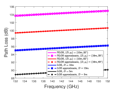
Figure 2: The overall pathloss $1/|\alpha_{\ell}(\Delta)|^{2}$ (dB) versus the operating frequency $(f_{c}+\Delta)$ in sub-THz bands, with the distance $D$ and $f_{c}=142$ GHz. For the NLOS path, the angle of reflection $\varphi_{i}$, the refractive index = $2.24-j0.025$, and $\sigma_{r}=0.088\times 10^{-3}$m are considered [6, 7, 52].

II-C Hybrid Transceiver and Signal Model

To facilitate the trade-off between performance and hardware cost, we consider a single-user hybrid transceiver design for MIMO-OFDM systems with $N_{t}^{RF}$ and $N_{r}^{RF}$ RF chains at the transmitter and receiver, respectively, as shown in Fig. 3. We can extend our work to the downlink multi-user scenario by viewing the link between the base station and each user as a single-user scenario. The fully connected network of phase shifters is implemented in the RF precoder and combiner. Our proposed training framework in Section III-A is general and applicable to the new hybrid structures [11, 53] that consider the beam squint effect. On a MIMO-OFDM system with $K_{o}$ subcarriers, we denote the MIMO channel on the $k$-th subcarrier as $\mathbf{H}_{k}\!=\!\mathbf{H}(\Delta_{k})$, where ${\Delta_{k}\!=\!(k\!-\!\frac{K_{o}+1}{2})\frac{B}{K_{o}}}$ is the baseband frequency of the $k$-th subcarrier.

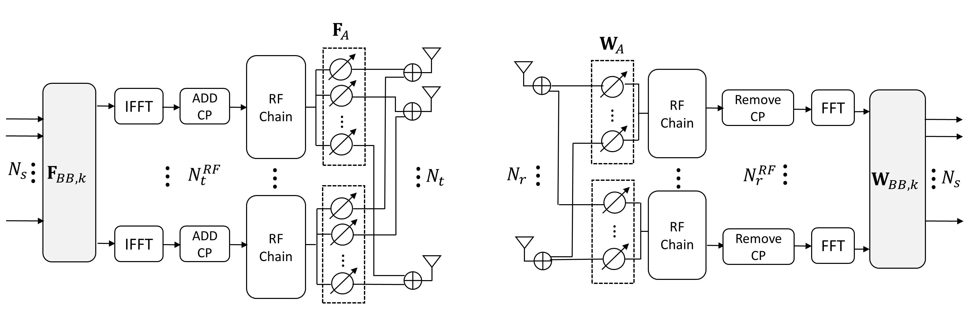
Figure 3: The MIMO-OFDM system with hybrid transceiver architecture [15, 11].

The transmitter sends the signal on the $k$-th subcarrier at the $\nu$-th subframe, denoted as

$$\mathbf{x}_{k,\nu}=\mathbf{F}_{A}\mathbf{F}_{BB,k}\mathbf{s}_{k,\nu}\in\mathbb{C}^{N_{t}\times 1},$$ (12)

where $\mathbf{s}_{k,\nu}\in\mathbb{C}^{N_{s}\times 1}$ is the baseband signal on the $k$-th subcarrier at the $\nu$-th subframe, $\mathbf{F}_{A}\in\mathbb{C}^{N_{t}\times N^{RF}_{t}}$ is a frequency-flat analog precoder, and $\mathbf{F}_{BB,k}\in\mathbb{C}^{N^{RF}_{t}\times N_{s}}$ is the baseband precoders for subcarrier $k$. At the receiver, the signal is received by the frequency-flat analog combiner $\mathbf{W}_{A}\in\mathbb{C}^{N_{r}\times N^{RF}_{r}}$ and then processed through the cyclic prefix removal and the discrete Fourier transform. The baseband combiner $\mathbf{W}_{BB,k}\in\mathbb{C}^{N^{RF}_{r}\times N_{s}}$ is processed for subcarrier $k$, yielding the received signal on the $k$-th subcarrier at the $\nu$-th subframe as

$$\mathbf{y}_{k,\nu}=\mathbf{W}_{BB,k}^{H}\mathbf{W}_{A}^{H}\mathbf{H}_{k}\mathbf{F}_{A}\mathbf{F}_{BB,k}\mathbf{s}_{k,\nu}+\mathbf{W}_{BB,k}^{H}\mathbf{W}_{A}^{H}\mathbf{v}_{k,\nu},$$ (13)

where $\mathbf{v}_{k,\nu}\in\mathbb{C}^{N_{r}\times 1}$ is the additive noise vector, with independent and identically distributed (i.i.d.) zero-mean complex Gaussian components with variance $\sigma_{n}^{2}$. Note that the hybrid precoder ($\mathbf{F}_{A}$/$\mathbf{F}_{BB,k}$) and combiner ($\mathbf{W}_{A}$/$\mathbf{W}_{BB,k}$) can be chosen differently on distinct subframes.

II-D Extended Virtual Representation of the MIMO Channel

Using the uniform antenna array assumption, the MIMO channel can be formulated as an extended virtual representation [54]. For the UPA at the receiver, we consider the physical AOA of interest as $(\theta_{pr},\theta_{ar})\in[-\pi/2,\pi/2)\times[-\pi,\pi)$. Assuming half wavelength antenna spacing $(\frac{d}{\lambda_{c}}=\frac{d}{c/f_{c}}=0.5)$, the beam direction region of interest is $(\psi_{hr},\psi_{vr})\in[-0.5,0.5)\times[-0.5,0.5)$. We assume that the horizontal (vertical) spatial AOAs take values from the uniform grid $\mathcal{G}_{hR}$ $(\mathcal{G}_{vR})$ of size $G_{hr}\geq L$ $(G_{vr}\geq L)$, given by

$$\mathcal{G}_{\rho R}=\bigg{\{}\psi_{i_{\rho}}=\frac{i_{\rho}-\frac{G_{\rho r}+1}{2}}{G_{\rho r}},\ i_{\rho}=1,\dots,G_{\rho r}\bigg{\}},$$ (14)

for $\rho\in\{h,v\}$. We define the grid of the receive UPA vectors as $\mathcal{G}_{R}=\mathcal{G}_{hR}\times\mathcal{G}_{vR}$, whose size $\lvert\mathcal{G}_{R}\rvert$ is $G_{r}=G_{hr}G_{vr}$. We construct the receive array response matrix on the $k$-th subcarrier by collecting the spatial-frequency UPA vectors with the AOAs taking values on $\mathcal{G}_{R}$ as

$$\mathbf{A}_{R,k}(:,i_{r})=\mathbf{a}_{N_{hr}}(\psi_{i_{h}};\Delta_{k})\otimes\mathbf{a}_{N_{vr}}(\psi_{i_{v}};\Delta_{k})\in\mathbb{C}^{N_{r}\times G_{r}},$$ (15)

where $i_{r}\!=\!(i_{h}-1)G_{vr}+i_{v}$ with $(\psi_{i_{h}},\psi_{i_{v}})\!\in\!\mathcal{G}_{R}$. Similarly, for the UPA at the transmitter, we assume the horizontal (vertical) spatial AODs take values from the uniform grid $\mathcal{G}_{hT}$ ($\mathcal{G}_{vT}$) of size $G_{ht}\geq L$ ($G_{vt}\geq L$). The grids $\mathcal{G}_{hT}$ and $\mathcal{G}_{vT}$ are constructed as in (14) by substituting $(G_{ht},G_{vt})$ for $(G_{hr},G_{vr})$, and the grid of the transmit UPA vectors is defined as $\mathcal{G}_{T}=\mathcal{G}_{hT}\times\mathcal{G}_{vT}$, whose size $\lvert\mathcal{G}_{T}\rvert$ is $G_{t}=G_{ht}G_{vt}$. By collecting the spatial-frequency UPA vectors with the AODs taking values on $\mathcal{G}_{T}$, we write the transmit array response matrix on the $k$-th subcarrier as

$$\mathbf{A}_{T,k}(:,i_{t})=\mathbf{a}_{N_{ht}}(\psi_{i_{h}};\Delta_{k})\otimes\mathbf{a}_{N_{vt}}(\psi_{i_{v}};\Delta_{k})\in\mathbb{C}^{N_{t}\times G_{t}},$$ (16)

where $i_{t}=(i_{h}-1)G_{vt}+i_{v}$ with $(\psi_{i_{h}},\psi_{i_{v}})\in\mathcal{G}_{T}$.

In this work, we consider a frame-based system, where each frame consists of $T_{c}$ subframes (channel uses). Assuming the frame duration is smaller than the channel coherence time, the channel remains constant in each frame, i.e., the common block-fading assumption. At the $F\textrm{-th}$ frame, the MIMO channel on the $k$-th subcarrier has an extended virtual representation [54] as

$$\mathbf{H}_{k}^{(F)}=\mathbf{A}_{R,k}\mathbf{D}_{k}^{(F)}\mathbf{A}_{T,k}^{H},$$ (17)

where $\mathbf{D}_{k}^{(F)}\in\mathbb{C}^{G_{r}\times G_{t}}$ is the beamspace channel matrix whose non-zero elements are located in positions corresponding to the spatial AOAs/AODs of the channel paths. Due to the mismatch between the spatial AOAs/AODs and the corresponding quantized values, a grid-mismatch error may exist but can be diminished if the grid sizes $(G_{hr},G_{vr},G_{ht},G_{vt})$ are chosen sufficiently large, which comes with a prohibitive computational complexity. In Section IV-B, we will design a sequential search method using hierarchical codebooks that allows mitigating the grid-mismatch problem with reduced computational complexity. The impact of grid-mismatch is numerically evaluated in Fig. 8, which shows the degradation of the channel estimation using small grid sizes. With the compact antenna deployments and the limited scattering of the sub-THz channel, the MIMO channels are spatially correlated and focus on certain spatial directions. The work [26] shows that the channel of a sub-THz band (140GHz) has an average of 6 clusters and 4 MPCs/cluster, whereas the mmWave band (28GHz) has an average of 8 clusters and 5 MPCs/cluster. Hence, the beamspace channel matrix $\mathbf{D}_{k}^{(F)}$ tends to be sparse. We assume that $\mathbf{D}_{k}^{(F)}$ has at most $L\!<\!G_{r}G_{t}$ non-zero elements, and the remaining elements are negligible.

We define the channel support of the $F$-th frame as $\Omega^{(F)}=\{(i_{r},i_{t}):\mathbf{{D}}_{k}^{(F)}(i_{r},i_{t})\!\neq\!0\},$ which is the indices set of the dominant elements in $\mathbf{{D}}_{k}^{(F)}$. The channel support is independent of the subcarrier $k$ since we construct the array response matrix $\mathbf{A}_{R,k}$, ($\mathbf{{A}}_{T,k}$) based on the same uniform grid $\mathcal{G}_{R}$ ($\mathcal{G}_{T}$) containing the quantized spatial AOAs (AODs). For the massive MIMO system, the channel support is mainly determined by the deployment geometry, hardware, and the time-varying effects of the propagation environment on the electromagnetic wave [29, 30].

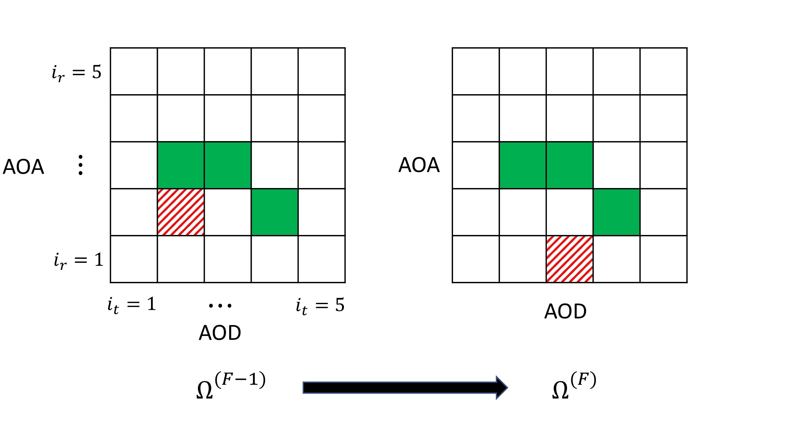
Figure 4: The evolution of beamspace channel with $(L,L_{cm})=(4,3)$ is illustrated. Between two consecutive frames, the green and red elements represent the common and changing elements, respectively.

In a frame-based system, the time-varying channel is approximated as fixed over the duration of a frame but may change across subsequent frames. With the temporal correlation, the channel support varies slowly over time, meaning that $\Omega^{(F-1)}$ and $\Omega^{(F)}$ share many common elements [31]. We assume $L_{cm}$ is the minimum number of channel elements shared between $\Omega^{(F-1)}$ and $\Omega^{(F)}$, denoted as $\lvert\Omega^{(F)}\cap\Omega^{(F-1)}\rvert\!\geq\!L_{cm}$, i.e., the AOA-AOD pairs that remain fixed between the consecutive frames. Given a fixed number of channel paths $L\geq L_{cm}$, there are at most $L-L_{cm}$ paths changing from one frame to the next. In Fig. 4, an example of the channel support evolution is illustrated, where the colored and white elements denote the dominant (non-zero) and negligible (zero) channel elements, respectively. For a slowly-varying channel with $L\!=\!4$ paths, the channel supports ${\Omega}^{(F-1)}$ and ${\Omega}^{(F)}$ share $L_{cm}\!=\!3$ common elements (shown in green), so only one path may change from one frame to the next (shown in red). This structure enables the LS-CS approach [45, 46] to reduce the training overhead, discussed in Section III.

III Proposed LS-CS Channel Training

In this section, we propose support tracking-based channel training for dual-wideband MIMO-OFDM systems. Section III-A depicts the beam training model, and Section III-B introduces the channel training protocol. Section III-C proposes a two-stage MMV-LS-CS (TS) channel estimation, and Section III-D proposes an MMV FISTA-based (M-FISTA) channel estimation.

III-A Beam Training Scheme

With each frame divided into $T_{c}$ equal-sized subframes, we assume that $T_{p}$ subframes are used for pilot-based channel training and the remaining $T_{c}\!-\!T_{p}$ subframes are used for data transmission. For the pilot transmission, we exploit $K_{p}\!<\!K_{o}$ subcarriers with a comb-type arrangement, i.e., $\mathcal{P}\!=\!\left\{1+(i-1)\delta_{p}:i=1,\dots,K_{p},\ \delta_{p}=\lceil{K_{o}}/{K_{p}}\rceil\right\}$, and the remaining subcarriers are used for data transmission. On the $k$-th subcarrier, the transmitter sends the precoded signal at the $\nu$-th subframe, and the receiver combines the measurement signal at the $q$-th stream by the combining vector $\mathbf{w}_{k,q}$. Assuming that the transmitter employs distinct precoded pilots of $T_{p}$ subframes in length and the receiver combines the signal into $Q_{p}$ streams, the $Q_{p}\times T_{p}$ combined signal on the $k$-th subcarrier, $k\in\mathcal{P}$, is denoted as

$$\mathbf{Y}_{k}=\mathbf{W}_{k}^{H}\mathbf{H}_{k}\mathbf{X}_{k}+\mathbf{\tilde{V}}_{k}=(\mathbf{A}_{R,k}^{H}\mathbf{W}_{k})^{H}\mathbf{D}_{k}(\mathbf{A}_{T,k}^{H}\mathbf{X}_{k})+\mathbf{\tilde{V}}_{k},$$ (18)

where $\mathbf{W}_{k}=[\mathbf{w}_{k,1},\dots,\mathbf{w}_{k,Q_{p}}]$ and $\mathbf{X}_{k}=[\mathbf{x}_{k,1},\dots,\mathbf{x}_{k,T_{p}}]$ are the measurement and pilot matrices, respectively. We denote the combined noise matrix as $\mathbf{\tilde{V}}_{k}=\mathbf{W}_{k}^{H}\mathbf{V}_{k}$, where $\mathbf{V}_{k}=[\mathbf{v}_{k,1},\dots,\mathbf{v}_{k,T_{p}}]$. With the extended virtual representation of the MIMO channel (17), we have a combined signal form (18). For the channel training, we adopt the random beamforming method [19, 15] to design the pilot and measurement matrices, i.e., $\mathbf{X}_{k}{(m,n)}\!=\!\frac{e^{j\zeta_{m,n}}}{\sqrt{N_{t}}},\ \zeta_{m,n}\!\sim\!\mathcal{U}(0,2\pi)$ and $\mathbf{W}_{k}{(m,n)}\!=\!\frac{e^{j\eta_{m,n}}}{\sqrt{N_{r}}},\ \eta_{m,n}\!\sim\!\mathcal{U}(0,2\pi)$. With sufficiently large $N_{r}$ and $N_{t}$, the elements of $\mathbf{A}_{R,k}^{H}\mathbf{W}_{k}$ and $\mathbf{A}_{T,k}^{H}\mathbf{X}_{k}$ are approximately i.i.d. $\mathcal{CN}(0,1/N_{r})$ (respectively, $\mathcal{CN}(0,1/N_{t})$) according to the central limit theorem [19, Appendix B], leading to the successful sparse recovery condition [55].

The hybrid transceiver is widely employed in mmWave and sub-THz communications, so we design the measurement and pilot matrices adopting the random beamforming method (discussed in the previous paragraph) based on the hybrid transceiver structure. For simplicity, we assume the number of subframes $T_{p}$ and the number of streams $Q_{p}$ satisfy $T_{p}\!=\!N_{ST}N_{t}^{RF}$ and $Q_{p}\!=\!N_{SR}N_{r}^{RF}$, for some $N_{ST},N_{SR}\!\in\!\mathbb{N}$, but the analysis can be generalized by considering $\mathbf{X}_{k}$ and $\mathbf{W}_{k}$ in (18). Then, we design a sequence of measurement matrices $\mathbf{W}_{k}\!=\!\left[\mathbf{W}_{k,1},\cdots,\mathbf{W}_{k,N_{SR}}\right]\!\in\!\mathbb{C}^{N_{r}\times Q_{p}}$ and of pilot matrices $\mathbf{X}_{k}\!=\!\left[\mathbf{X}_{k,1},\cdots,\mathbf{X}_{k,N_{ST}}\right]\!\in\!\mathbb{C}^{N_{t}\times T_{p}}$ so as to match the beamforming values generated randomly as explained in the previous paragraph. With the hybrid receiver structure, each submatrix $\mathbf{W}_{k,i}\!=\!\mathbf{W}_{A,i}\mathbf{W}_{BB,k,i}\!\in\!\mathbb{C}^{N_{r}\times N_{r}^{RF}},i\!=\!1,\dots,N_{SR}$ is obtained by setting $\mathbf{W}_{BB,k,i}\!=\!\mathbf{I}_{N_{r}^{RF}}$ and $\mathbf{W}_{A,i}{(m,n)}\!=\!\frac{e^{j\eta_{m,n}}}{\sqrt{N_{r}}},\ \eta_{m,n}\!\sim\!\mathcal{U}(0,2\pi)$. Similarly, each submatrix $\mathbf{X}_{k,i}\!=\!\mathbf{F}_{A,i}\mathbf{F}_{BB,k,i}\mathbf{S}_{k,i}\!\in\!\mathbb{C}^{N_{t}\times N_{t}^{RF}},i=1,\dots,N_{ST}$ is obtained by setting $\mathbf{F}_{BB,k,i}\!=\!\mathbf{S}_{k,i}\!=\!\mathbf{I}_{N_{t}^{RF}}$ and $\mathbf{F}_{A,i}{(m,n)}\!=\!\frac{e^{j\zeta_{m,n}}}{\sqrt{N_{t}}},\ \zeta_{m,n}\!\sim\!\mathcal{U}(0,2\pi)$. Our work focuses on the design of the channel training, and this configuration justifies our proposed channel training in the hybrid transceiver structure.

III-B Channel Training Protocol

We introduce the protocol of the support tracking-based channel training by exploiting the temporal correlation, shown in Fig. 5. In each frame, support tracking-based channel training is used to estimate the channel aided by the previous channel support. Note that the quality of the estimated previous channel support is crucial to the channel estimation performance. An inaccurate previous channel support might deteriorate the performance of the support tracking-based approach because more channel elements are required to be estimated in the CS stage. In the first frame, we initialize the previous channel support as an empty set since no prior CSI is available. In the following frames, the previous channel support is derived from the estimated channel in the preceding frame. To ensure satisfactory quality, we check the residual signal of the support tracking-based channel training. If its magnitude is smaller than a predefined threshold, we continue the support tracking-based channel training on the next frame. Otherwise, the estimated previous channel support is considered unreliable, and the channel training procedure is reset by setting the previous channel support as an empty set.

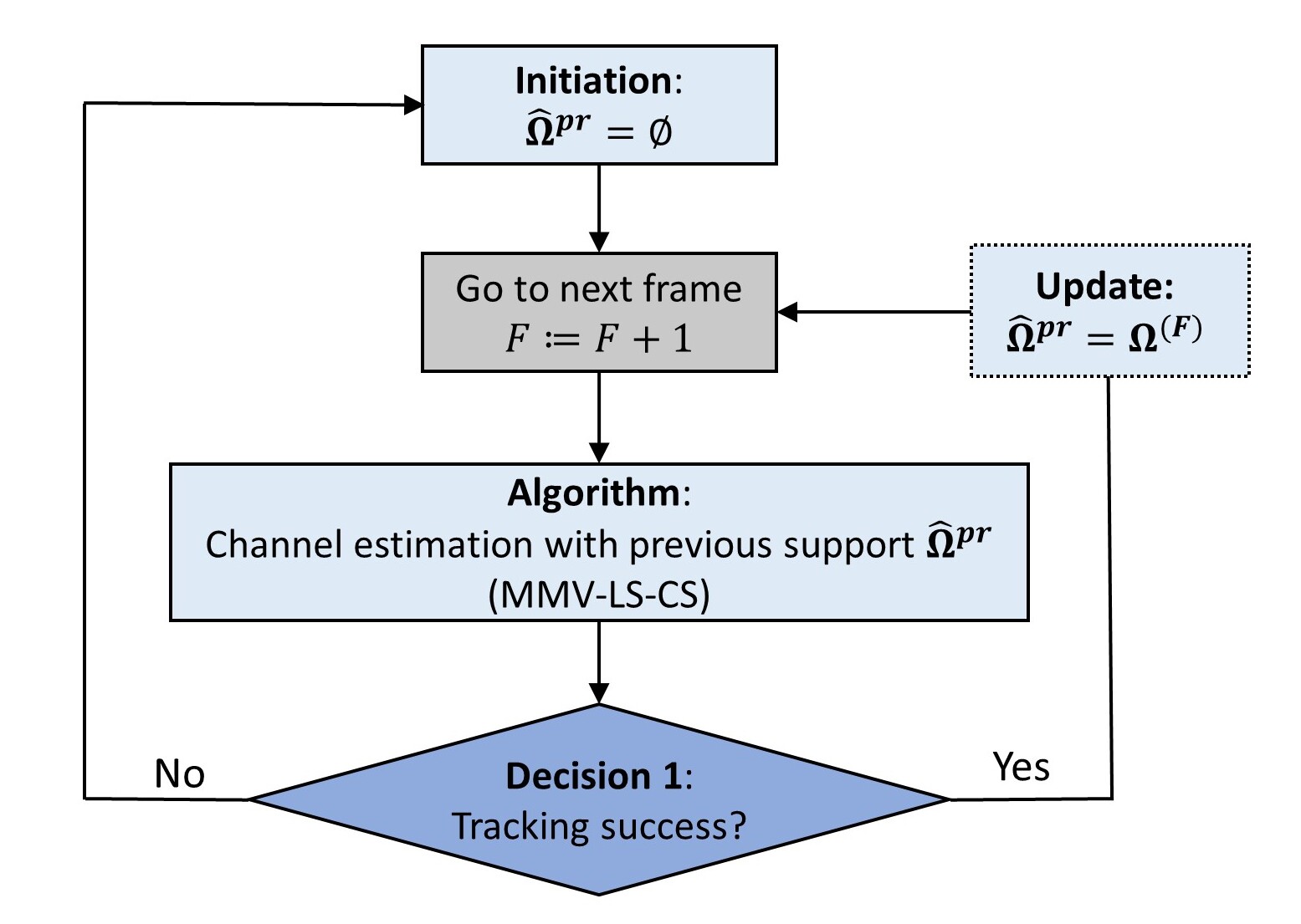
Figure 5: The proposed channel training protocol.

III-C Two-Stage MMV-LS-CS Channel Estimation (TS)

Our goal is to develop an approach to reduce the overhead of channel training using the estimated previous channel support $\hat{\Omega}^{pr}$, where the real previous channel support ${\Omega}^{pr}$ is unknown. We estimate the spatial AOAs/AODs of the dominant channel paths and then refine the time delays and path coefficients of the estimated paths. Given the training signal (18) with the measurement and pilot matrices $(\mathbf{W}_{k},\mathbf{X}_{k})$ and the relationship $\textrm{vec}(\mathbf{ABC})=(\mathbf{C}^{\top}\otimes\mathbf{A})\textrm{vec}(\mathbf{B})$, we have the vectorization of $\mathbf{Y}_{k}$ as

$$\mathbf{y}_{k}=\textrm{vec}(\mathbf{Y}_{k})=\mathbf{\Theta}_{k}\mathbf{z}_{k}+\mathbf{\tilde{v}}_{k},$$ (19)

where $\mathbf{\Theta}_{k}=(\mathbf{A}_{T,k}^{H}\mathbf{X}_{k})^{\top}\otimes(\mathbf{A}_{R,k}^{H}\mathbf{W}_{k})^{H}$ is the dictionary matrix on the $k$-th subcarrier, $\mathbf{z}_{k}=\textrm{vec}(\mathbf{D}_{k})$ and $\mathbf{\tilde{v}}_{k}=\textrm{vec}(\mathbf{\tilde{V}}_{k})$. We introduce the two-stage MMV-LS-CS (TS) algorithm for the time-varying MIMO-OFDM channel estimation, which separates the channel training into two stages: MMV-LS and MMV-CS. MMV-LS exploits the slowly-varying channel by performing the LS estimate on the estimated previous channel support. Next, MMV-CS applies a CS-based approach to the LS residual, expected to be sparse since most dominant channel elements have been estimated in MMV-LS. The TS algorithm is shown in Algorithm 1 and operates as follows.

First, MMV-LS estimates the beamspace channel elements corresponding to the estimated previous channel support $\hat{\Omega}^{pr}$. We denote the set of column indices (of $\mathbf{\Theta}_{k}$) corresponding to $\hat{\Omega}^{pr}$ as $\mathcal{Q}=\{(i_{t}-1)G_{r}+i_{r}:(i_{r},i_{t})\in\hat{\Omega}^{pr}\}$. The beamspace channel vectors share common support across the subcarriers, enabling the MMV to estimate the dominant paths. The MMV-LS algorithm is initialized as $\Gamma=\emptyset$ (line 3). Then, $\Gamma$ is reconstructed recursively by collecting the indices from $\mathcal{Q}$, which leads to the minimum residual error after orthogonalization, until $\lvert\Gamma\rvert=L_{cm}$ (lines 4-7). The estimated beamspace channel in MMV-LS is derived as $[\mathbf{\hat{z}}_{k}^{LS}]_{\Gamma}=[\mathbf{\Theta}_{k}]_{\Gamma}^{+}\textbf{y}_{k}$ and $[\mathbf{\hat{z}}_{k}^{LS}]_{\Gamma^{c}}=0$ (line 8), where $\Gamma^{c}=\{1,\dots,G_{r}G_{t}\}\backslash\Gamma$.

Secondly, MMV-CS executes a CS-based approach on the LS residual signal obtained by subtracting the effect of the MMV-LS estimated beamspace channel $\mathbf{\hat{z}}_{k}^{LS}$ (line 10), given as

$$\mathbf{y}_{k}^{CS}=\textbf{y}_{k}-\mathbf{\Theta}_{k}\mathbf{\hat{z}}_{k}^{LS}=\mathbf{\Theta}_{k}\mathbf{z}_{k}^{CS}+\mathbf{\tilde{v}}_{k},$$

where $\mathbf{z}_{k}^{CS}=\mathbf{z}_{k}-\mathbf{\hat{z}}_{k}^{LS}$ is expected to be sparser than $\mathbf{z}_{k}$ since most dominant path components ($L_{cm}$ out of $L$) are expected to be detected in $\mathbf{\hat{z}}_{k}^{LS}$, so that $\mathbf{z}_{k}^{CS}$ is expected to have only $(L-L_{cm})$ non-zero components. The sparse recovery problem on the pilot subcarriers is formulated as

$$\arg\min\limits_{\mathbf{z}_{k}^{CS}}\ \sum\nolimits_{k\in\mathcal{P}}\lVert\mathbf{z}_{k}^{CS}\rVert_{1},\ \textrm{s.t. }\lVert\mathbf{y}_{k}^{CS}-\mathbf{\Theta}_{k}\mathbf{z}_{k}^{CS}\rVert_{2}\leq\epsilon,$$ (20)

where $\epsilon>0$ is a constant threshold. Among many available sparse recovery algorithms using the common channel support across subcarriers, we adopt the simultaneous OMP algorithm (SOMP) [56]. The algorithm is initialized as $\Upsilon\!=\!\emptyset$ and the residual $\mathbf{r}_{k}\!=\!\mathbf{y}_{k}^{CS},\ k\in\mathcal{P}$ (line 10). Then, the set $\Upsilon$ is constructed by collecting the index of the column (of $\mathbf{\Theta}_{k}$) having the largest correlation with $\mathbf{r}_{k}$ (line 13). In each iteration, the residual $\mathbf{r}_{k}$ is updated by removing the channel effect of the indices in $\Upsilon$ (line 14-15). The TS algorithm stops when it reaches $t_{max}$ iterations or the relative error of the residual signal $\varepsilon_{t}<\epsilon$ (line 12). The estimated beamspace channel in MMV-CS is derived as $[\mathbf{\hat{z}}_{k}^{CS}]_{\Upsilon}=[\mathbf{\Theta}_{k}]_{\Upsilon}^{+}\textbf{y}_{k}^{CS}\textrm{ and }[\mathbf{\hat{z}}_{k}^{CS}]_{\Upsilon^{c}}=0$ (line 18), where $\Upsilon^{c}=\{1,\dots,G_{r}G_{t}\}\backslash\Upsilon$.

Algorithm 1 Two-stage MMV-LS-CS Channel Estimation (TS).

1:measurement $\mathbf{Y}_{k}$, dictionary matrix $\mathbf{\Theta}_{k}$, estimated previous channel support $\hat{\Omega}^{pr}$

2:estimated channel $\mathbf{\hat{H}}_{k}$

3:MMV-LS aided by the estimated previous channel support

4:$\mathbf{y}_{k}=\text{vec}(\mathbf{Y}_{k}),\ k\in\mathcal{P}$;

5:$\Gamma=\emptyset$; $\mathcal{Q}=\{(i_{t}-1)G_{r}+i_{r}:(i_{r},i_{t})\in\hat{\Omega}^{pr}\}$;

6:while $\lvert\Gamma\rvert<L_{cm}$ and $\hat{\Omega}^{pr}\neq\emptyset$ do

7:   $j^{*}=\arg\min\limits_{j\in\mathcal{Q}\backslash\Gamma}\sum_{k\in\mathcal{P}}\lVert\mathbf{y}_{k}-[\mathbf{\Theta}_{k}]_{\Gamma\cup{j}}[\mathbf{\Theta}_{k}]_{\Gamma\cup{j}}^{+}\mathbf{y}_{k}\rVert_{F}^{2};$

8:   $\Gamma\coloneqq\Gamma\cup j^{*};$

9:end while

10:$[\mathbf{\hat{z}}_{k}^{LS}]_{\Gamma}=[\mathbf{\Theta}_{k}]_{\Gamma}^{+}\textbf{y}_{k}\textrm{ and }[\mathbf{\hat{z}}_{k}^{LS}]_{\Gamma^{c}}=0,\ k\in\mathcal{P}$;

11:

12:MMV-CS on the LS residual

13:$\mathbf{y}_{k}^{CS}=\textbf{y}_{k}-\mathbf{\Theta}_{k}\mathbf{\hat{z}}_{k}^{LS},\ k\in\mathcal{P}$; $\Upsilon=\emptyset$; $\mathbf{r}_{k,t}=\mathbf{y}_{k}^{CS},\ k\in\mathcal{P}$;

14:$\mathcal{J}=\{1,\dots,G_{r}G_{t}\}$; $\varepsilon_{t}=\infty$;

15:while $\varepsilon_{t}>\epsilon$ and $t<t_{max}$ do

16:   $\Upsilon\coloneqq\Upsilon\cup\arg\max_{j\in\mathcal{J}\backslash\Upsilon}\sum_{k\in\mathcal{P}}\lvert\mathbf{\Theta}_{k}(:,j)^{H}\mathbf{r}_{k,t}\rvert^{2};$

17:   $\mathbf{\hat{g}}_{k}=\arg\min_{\mathbf{g}}\lVert\mathbf{y}_{k}^{CS}-[\mathbf{\Theta}_{k}]_{\Upsilon}\mathbf{g}\rVert_{F}^{2},\ k\in\mathcal{P};$

18:   $\mathbf{r}_{k,t+1}=\mathbf{y}_{k}^{CS}-[\mathbf{\Theta}_{k}]_{\Upsilon}\mathbf{\hat{g}}_{k},\ k\in\mathcal{P};$

19:   $\varepsilon_{t+1}=\frac{1}{\lvert\mathcal{P}\rvert}\sum_{k\in\mathcal{P}}\lVert\mathbf{r}_{k,t+1}-\mathbf{r}_{k,t}\rVert_{F}^{2}$; $t\coloneqq t+1$;

20:end while

21:$[\mathbf{\hat{z}}_{k}^{CS}]_{\Upsilon}=[\mathbf{\Theta}_{k}]_{\Upsilon}^{+}\textbf{y}_{k}^{CS}\textrm{ and }[\mathbf{\hat{z}}_{k}^{CS}]_{\Upsilon^{c}}=0,\ k\in\mathcal{P};$

22:

23:Combine the detections from MMV-LS and MMV-CS

24:$\Xi\!=\!\{i\!:\!i\in\{1,\dots,G_{r}G_{t}\},\ \frac{1}{\lvert\mathcal{P}\rvert}\sum\limits_{k\in\mathcal{P}}\lvert(\mathbf{\hat{z}}_{k}^{LS}+\mathbf{\hat{z}}_{k}^{CS})_{i}\rvert\neq 0\}$;

25:Derive the estimated current channel support

26:$[\mathbf{\hat{z}}_{k}^{det}]_{\Xi}=[\mathbf{\Theta}_{k}]_{\Xi}^{+}\textbf{y}_{k},\ [\mathbf{\hat{z}}_{k}^{det}]_{\Xi^{c}}=0,\ k\in\mathcal{P};$

27:$\mathbf{z}_{eq}=\frac{1}{\lvert\mathcal{P}\rvert}\sum_{k\in\mathcal{P}}\lvert\mathbf{\hat{z}}_{k}^{det}\rvert$;

28:$\tilde{\Xi}=\arg\max_{\tilde{\Xi}\subset\Xi,\ \lvert\tilde{\Xi}\rvert=L^{\prime}}\sum_{i\in\tilde{\Xi}}(\mathbf{z}_{eq})_{i}$;

29:

30:Reconstruct $\mathbf{\hat{H}}_{k}$ by Algorithm 3 with $(\mathbf{Y}_{k},\mathbf{\Theta}_{k},\tilde{\Xi})$;

As discussed in [46], with the $\ell_{1}$-norm minimization subject to the noise constraint (e.g., MMV-CS in (20)), the estimate $\mathbf{\hat{z}}_{k}^{CS}$ tends to be biased towards zero. Also, MMV-CS might lead to false detections of the components, whose beamspace channel value is zero but is detected as non-zero due to noise or detection error. To reduce the bias and improve performance in practical settings, we derive the channel support by combining the new detection $\mathbf{\hat{z}}_{k}^{CS}$ in MMV-CS with the estimated $\mathbf{\hat{z}}_{k}^{LS}$ from MMV-LS (line 20) as

$$\Xi=\Big{\{}i:i\in\{1,\dots,G_{r}G_{t}\},\ \frac{1}{\lvert\mathcal{P}\rvert}\sum_{k\in\mathcal{P}}\lvert(\mathbf{\hat{z}}_{k}^{LS}+\mathbf{\hat{z}}_{k}^{CS})_{i}\rvert\neq 0\Big{\}}.$$

The LS estimate on $\Xi$ is computed as $[\mathbf{\hat{z}}_{k}^{det}]_{\Xi}=[\mathbf{\Theta}_{k}]_{\Xi}^{+}\textbf{y}_{k}$ and $[\mathbf{\hat{z}}_{k}^{det}]_{\Xi^{c}}=0,\ k\in\mathcal{P},$ where $\Xi^{c}=\{1,\dots,G_{r}G_{t}\}\backslash\Xi$. Next, we derive the estimated channel support by collecting the indices of the largest $L^{\prime}$ values of $\mathbf{z}_{eq}=\frac{1}{\lvert\mathcal{P}\rvert}\sum_{k\in\mathcal{P}}\lvert\mathbf{\hat{z}}_{k}^{det}\rvert$, given by

$$\tilde{\Xi}=\arg\max_{\tilde{\Xi}\subset\Xi,\ \lvert\tilde{\Xi}\rvert=L^{\prime}}\sum\nolimits_{i\in\tilde{\Xi}}\lvert(\mathbf{z}_{eq})_{i}\rvert.$$

where $L^{\prime}\!=\!\lfloor mL\rfloor$ with $m\geq 1$. We choose $m\!=\!4$ to account for the potentially missed and false detections. The set $\tilde{\Xi}$ becomes the estimated previous channel support in the next frame.

Lastly, we apply the channel refinement algorithm (Algorithm 3, which will be introduced in Section IV-A) to reconstruct the estimated channel $\mathbf{\hat{H}}_{k}$. The channel refinement algorithm improves the channel estimation performance by deriving the path coefficients and time delays of the estimated paths corresponding to the estimated channel support $\tilde{\Xi}$ from the received signal jointly on the pilot subcarriers.

Note that the TS algorithm collects $L_{cm}$ elements from the estimated previous channel support $\hat{\Omega}^{pr}$ in MMV-LS. Due to the potential estimation errors in the preceding frame, $\hat{\Omega}^{pr}$ is possibly inaccurate and contains less than $L_{cm}$ correct channel elements. With an inaccurate $\hat{\Omega}^{pr}$, MMV-LS would collect wrong channel elements inducing the estimation error, and MMV-CS requires estimating an increased number of channel elements. To address this issue, we develop a joint MMV-LS-CS approach (M-FISTA) in the next subsection to do the channel estimation, which does not require the exact number of the correct channel elements in $\hat{\Omega}^{pr}$.

III-D MMV FISTA-based Channel Estimation (M-FISTA)

We propose a joint MMV-LS-CS using the framework of FISTA [47] instead of doing the MMV-LS-CS in two stages. Given the estimated previous channel support $\Gamma\!=\!\{(i_{t}-1)G_{r}\!+\!i_{r}:(i_{r},i_{t})\in\hat{\Omega}^{pr}\}$, by staking up the signal (19) over the subcarriers, we have the signal model as

$$\mathbf{\tilde{y}}=\mathbf{\Phi}_{A}\mathbf{\tilde{z}}^{LS}+\mathbf{\Phi}_{B}\mathbf{\tilde{z}}^{CS}+\mathbf{\tilde{v}},$$ (21)

where $\mathbf{\tilde{z}}^{LS}\!=\!\left[[\mathbf{z}_{1}]_{\Gamma}^{\top},\dots,[\mathbf{z}_{K_{p}}]_{\Gamma}^{\top}\right]^{\top}$, $\mathbf{\tilde{z}}^{CS}\!=\!\left[[\mathbf{z}_{1}]_{\Gamma^{c}}^{\top},\dots,[\mathbf{z}_{K_{p}}]_{\Gamma^{c}}^{\top}\right]^{\top}$, $\mathbf{\Phi}_{A}\!=\!\textrm{bdiag}\left(\left[\mathbf{\Theta}_{1}\right]_{\Gamma},\dots,\left[\mathbf{\Theta}_{K_{p}}\right]_{\Gamma}\right)$, $\mathbf{\Phi}_{B}=\textrm{bdiag}\left(\left[\mathbf{\Theta}_{1}\right]_{\Gamma^{c}},\dots,\left[\mathbf{\Theta}_{K_{p}}\right]_{\Gamma^{c}}\right)$, $\mathbf{\tilde{y}}\!=\![\mathbf{y}_{1}^{\top},\dots,\mathbf{y}_{K_{p}}^{\top}]^{\top}$ and $\mathbf{\tilde{v}}\!=\![\mathbf{\tilde{v}}_{1}^{\top},\dots,\mathbf{\tilde{v}}_{K_{p}}^{\top}]^{\top}$. For ease of exposition, we index the pilot subcarriers as $k=1,\dots,K_{p}$. For a vector $\mathbf{x}\in\mathbb{C}^{MN\times 1}$ with the subvectors $\mathbf{x}(1+i_{2}M:M+i_{2}M)\in\mathbb{C}^{M\times 1},\ i_{2}=0,\dots,N-1$ sharing the joint sparsity pattern, the mixed $\ell_{2}/\ell_{1}$ norm of $\mathbf{x}$ is defined as

$$\lVert\mathbf{x}\rVert_{2,1}=\sum_{i_{1}=1}^{M}\sqrt{\sum_{i_{2}=0}^{N-1}\left\lvert\mathbf{x}(i_{1}+i_{2}M)\right\rvert^{2}}.$$ (22)

We consider $(M,N)=(\lvert\Gamma\rvert,K_{p})$ for $\lVert\mathbf{\tilde{z}}^{LS}\rVert_{2,1}$ and $(M,N)=(\lvert\Gamma^{c}\rvert,K_{p})$ for $\lVert\mathbf{\tilde{z}}^{CS}\rVert_{2,1}$, respectively. The sparse recovery problem can be formulated as

$$\arg\min\limits_{\mathbf{\tilde{z}}^{LS},\ \mathbf{\tilde{z}}^{CS}}\ \frac{1}{2}\lVert\mathbf{\tilde{y}}-\mathbf{\Phi}_{A}\mathbf{\tilde{z}}^{LS}-\mathbf{\Phi}_{B}\mathbf{\tilde{z}}^{CS}\rVert^{2}$$

$$+\lambda_{1}\lVert\mathbf{\tilde{z}}^{LS}\rVert_{2,1}+\lambda_{2}\lVert\mathbf{\tilde{z}}^{CS}\rVert_{2,1},$$ (23)

where $\lambda_{1}$ and $\lambda_{2}$ are regularization numbers, determined by the non-zero entries in $\mathbf{\tilde{z}}^{LS},\mathbf{\tilde{z}}^{CS}$, that weight the penalty terms. The minimum number of the shared channel elements between the consecutive frames is $L_{cm}$ (out of $L$ paths), leading to different scales for $\lVert\mathbf{\tilde{z}}^{LS}\rVert_{2,1}$ and $\lVert\mathbf{\tilde{z}}^{CS}\rVert_{2,1}$. For a positive constant number $\lambda$, we choose $\lambda_{1}=\lambda\sqrt{\frac{1}{L_{cm}}}$ and $\lambda_{2}=\lambda\sqrt{\frac{1}{L-L_{cm}}}$ since $\lambda_{1}$ (respectively, $\lambda_{2}$) is inversely related to the scale of $\lVert\mathbf{\tilde{z}}^{LS}\rVert_{2,1}$ (respectively, $\lVert\mathbf{\tilde{z}}^{CS}\rVert_{2,1}$). Letting $\mathbf{\Phi}=[\mathbf{\Phi}_{A}\ \mathbf{\Phi}_{B}]$, $\mathbf{x}=[(\mathbf{\tilde{z}}^{LS})^{\top}\ (\mathbf{\tilde{z}}^{CS})^{\top}]^{\top}$, we have $f(\mathbf{x})=\frac{1}{2}\lVert\mathbf{\tilde{y}}-\mathbf{\Phi}\mathbf{x}\rVert^{2}$ and $g(\mathbf{x})=\lambda_{1}\lVert\mathbf{\tilde{z}}^{LS}\rVert_{2,1}+\lambda_{2}\lVert\mathbf{\tilde{z}}^{CS}\rVert_{2,1}$. The problem (23) can be viewed as a LASSO problem, formulated as

$$\arg\min\limits_{\mathbf{x}}\ F(\mathbf{x})=f(\mathbf{x})+g(\mathbf{x}),$$ (24)

where $f$ is a smooth, convex, and continuously differentiable function. For $f(\mathbf{x})$, we derive its gradient as $\nabla{f}(\mathbf{x})\!=\!\mathbf{\Phi}^{H}(\mathbf{\Phi}\mathbf{x}-\mathbf{\tilde{y}})$ and the Lipschitz constant equals to $\lVert\mathbf{\Phi}\rVert_{2}^{2}$. For the convex function $g:\mathbb{R}^{N}\rightarrow\mathbb{R}\cup\{\infty\}$ and $\eta\in\mathbb{R}$, the proximal operator of $\mathbf{x}$ associated with $\frac{1}{\eta}g$ is defined by $\textrm{prox}_{\frac{1}{\eta}g}(\mathbf{x})\!=\!\arg\min_{\mathbf{u}\in\mathbb{R}^{N}}\left\{g(\mathbf{u})\!+\!\frac{\eta}{2}\lVert\mathbf{u}\!-\!\mathbf{x}\rVert_{2}^{2}\right\}$, which is required to implement the FISTA. Given $\eta\!\geq\!\lVert\mathbf{\Phi}\rVert_{2}^{2}$, we derive the proximal operator of $\mathbf{x}$ associated with $\frac{1}{\eta}g$, given by

$$\text{prox}_{\frac{1}{\eta}g}(\mathbf{x})\!=\!\left[\text{prox}_{\frac{1}{\eta}\lambda_{1}\lVert\cdot\rVert_{2,1}}(\mathbf{\tilde{z}}^{LS})^{\top}\ \ \text{prox}_{\frac{1}{\eta}\lambda_{2}\lVert\cdot\rVert_{2,1}}(\mathbf{\tilde{z}}^{CS})^{\top}\right]^{\top}.$$

The operators $\text{prox}_{\frac{1}{\eta}\lambda_{1}\lVert\cdot\rVert_{2,1}}$ and $\text{prox}_{\frac{1}{\eta}\lambda_{2}\lVert\cdot\rVert_{2,1}}$ are the group-thresholding operators [57], given by

$$\text{prox}_{\frac{1}{\eta}\lambda_{1}\lVert\cdot\rVert_{2,1}}(\mathbf{\tilde{z}}^{LS}_{i})=\frac{\mathbf{\tilde{z}}^{LS}_{i}}{\lVert\mathbf{\tilde{z}}^{LS}_{i}\rVert_{2}}\max\Big{(}\lVert\mathbf{\tilde{z}}^{LS}_{i}\rVert_{2}-\frac{1}{\eta}\lambda_{1},0\Big{)},\$$

for $i=1,\dots,\lvert\Gamma\rvert,$ and

$$\text{prox}_{\frac{1}{\eta}\lambda_{2}\lVert\cdot\rVert_{2,1}}(\mathbf{\tilde{z}}^{CS}_{i})=\frac{\mathbf{\tilde{z}}^{CS}_{i}}{\lVert\mathbf{\tilde{z}}^{CS}_{i}\rVert_{2}}\max\Big{(}\lVert\mathbf{\tilde{z}}^{CS}_{i}\rVert_{2}-\frac{1}{\eta}\lambda_{2},0\Big{)},$$

for $i=1,\dots,\lvert\Gamma^{c}\rvert$. The vectors $\mathbf{\tilde{z}}^{LS}_{i}=[\mathbf{\tilde{z}}^{LS}(i)\ \mathbf{\tilde{z}}^{LS}(i+\lvert\Gamma\rvert)\ \cdots\ \mathbf{\tilde{z}}^{LS}(i+(K_{p}-1)\lvert\Gamma\rvert)]^{\top}$ and $\mathbf{\tilde{z}}^{CS}_{i}=[\mathbf{\tilde{z}}^{CS}(i)\ \mathbf{\tilde{z}}^{CS}(i+\lvert\Gamma^{c}\rvert)\ \cdots\ \mathbf{\tilde{z}}^{CS}(i+(K_{p}-1)\lvert\Gamma^{c}\rvert)]^{\top}$ are the subvectors of $\mathbf{\tilde{z}}^{LS}$ and $\mathbf{\tilde{z}}^{CS}$, respectively. The M-FISTA channel estimator is shown in Algorithm 2. With the estimated $\mathbf{x}_{u}$, the estimates of $\mathbf{\hat{z}}_{k}^{LS}$ and $\mathbf{\hat{z}}_{k}^{CS}$ can be derived with appropriate rearrangement (line 9). The M-FISTA algorithm stops when it reaches $U_{max}$ iterations or the relative error of the objective function $\lVert F(\mathbf{x}_{u})-F(\mathbf{x}_{u-1})\rVert<\epsilon$.

Algorithm 2 MMV FISTA-based Channel Estimation (M-FISTA).

1:measurement $\mathbf{\tilde{y}}$, dictionary matrix $\mathbf{\Phi}$, initial point $\mathbf{x}_{0}$, upper bound $\eta\geq\lVert\mathbf{\Phi}\rVert_{2}^{2}$

2:estimated channel $\mathbf{\hat{H}}_{k}$

3:Initialization: $u=1$, $\mathbf{q}_{1}=\mathbf{x}_{0}$, $t_{1}=1$, $\varepsilon=\infty$;

4:while $u<U_{max}$ and $\varepsilon>\epsilon$ do

5:   $\nabla f(\mathbf{q}_{u})=\mathbf{\Phi}^{H}(\mathbf{\Phi}\mathbf{q}_{u}-\mathbf{\tilde{y}})$;

6:   $\mathbf{x}_{u}=\text{prox}_{\frac{1}{\eta}g}(\mathbf{q}_{u}-\frac{1}{\eta}\nabla f(\mathbf{q}_{u}))$;

7:   $t_{u+1}=\frac{1+\sqrt{1+4t_{u}^{2}}}{2}$;

8:   $\mathbf{q}_{u+1}=\mathbf{x}_{u}+\frac{t_{u}-1}{t_{u+1}}(\mathbf{x}_{u}-\mathbf{x}_{u-1})$;

9:   $\varepsilon=\lvert F(\mathbf{x}_{u})-F(\mathbf{x}_{u-1})\rvert$; $u\coloneqq u+1$;

10:end while

11:Derive $\mathbf{\hat{z}}_{k}^{LS}$ and $\mathbf{\hat{z}}_{k}^{CS}$ from $\mathbf{x}_{u}$;

12:The support of $\mathbf{\Theta}_{k}^{(1)}$: $\Xi^{(1)}\!=\!\{i:\sum\limits_{k\in\mathcal{P}}\lvert(\mathbf{\hat{z}}_{k}^{LS}+\mathbf{\hat{z}}_{k}^{CS})_{i}\rvert\neq 0\}$;

13:

14:Enhance the beam resolution by sequential search method

15:$\Upsilon=\emptyset$; $\mathcal{R}=\emptyset$; $\mathbf{T}_{k}=[\ ]$, $\mathbf{r}_{k}=\mathbf{y}_{k},\ k\in\mathcal{P}$;

16:while $\lvert\Upsilon\rvert<L^{\prime}$ do

17:   $j_{1}^{*}=\arg\max\limits_{j\in\Xi^{(1)}\backslash\Upsilon}\sum\limits_{k\in\mathcal{P}}\lvert\mathbf{\Theta}_{k}^{(1)}(:,j)^{H}\mathbf{r}_{k}\rvert^{2}$; $\Upsilon:=\Upsilon\cup j_{1}^{*}$;

18:   Derive $(\hat{\psi}_{A}^{(1)},\hat{\psi}_{B}^{(1)},\hat{\psi}_{C}^{(1)},\hat{\psi}_{D}^{(1)})$ from $j_{1}^{*}$;

19:   Derive $(\hat{\psi}_{A}^{(M)},\hat{\psi}_{B}^{(M)},\hat{\psi}_{C}^{(M)},\hat{\psi}_{D}^{(M)})$ using (33)-(36);

20:   Derive $j_{2}^{*}$ from $(\hat{\psi}_{A}^{(M)},\hat{\psi}_{B}^{(M)},\hat{\psi}_{C}^{(M)},\hat{\psi}_{D}^{(M)})$; $\mathcal{R}:=\mathcal{R}\cup j_{2}^{*}$;

21:   $\mathbf{T}_{k}:=\Big{[}\mathbf{T}_{k}\ \mathbf{\Theta}_{k}^{(M)}(:,j_{2}^{*})\Big{]},\ k\in\mathcal{P}$;

22:   $\mathbf{r}_{k}=\mathbf{y}_{k}-\mathbf{T}_{k}\mathbf{T}_{k}^{+}\mathbf{y}_{k},\ k\in\mathcal{P}$;

23:end while

24:Derive $\tilde{\Xi}^{(M)}$ (i.e. the support of $\mathbf{\Theta}_{k}^{(M)}$) from $\mathcal{R}$;

25:

26:Reconstruct $\mathbf{\hat{H}}_{k}$ by Algorithm 3 with $(\mathbf{Y}_{k},\mathbf{\Theta}_{k}^{(M)},\tilde{\Xi}^{(M)})$;

Since the LASSO approach does not handle highly correlated variables well, we are not able to do the FISTA-based algorithm with dictionary matrices that have very large grid sizes, inducing a higher correlation between the atoms. Without additional processing, M-FISTA estimates the channel support with a low-resolution codebook (line 1-10), degrading the estimation accuracy due to the grid mismatch. To address the grid-mismatch issue, we apply a sequential search method with hierarchical codebooks (Section IV-B) to enhance the resolution of each estimated path. We construct the hierarchical codebook for the index selection on multiple levels, introduced in Section IV-B1. The first-level codebook $\mathbf{\Theta}_{k}^{(1)}$ is considered the low-resolution codebook, and the $M$-th level ($M\!>\!1$) codebook $\mathbf{\Theta}_{k}^{(M)}$ refers to the high-resolution codebook. We have the channel support (of $\mathbf{\Theta}_{k}^{(1)}$) by combining $\mathbf{\hat{z}}_{k}^{LS}$ with $\mathbf{\hat{z}}_{k}^{CS}$ as $\Xi^{(1)}\!=\!\{i\!:\!\sum\nolimits_{k\in\mathcal{P}}\lvert(\mathbf{\hat{z}}_{k}^{LS}+\mathbf{\hat{z}}_{k}^{CS})_{i}\rvert\!\neq\!0\}$ (line 10). Next, the algorithm is initialized as $\Upsilon=\emptyset$, $\mathcal{R}=\emptyset$, and the residual $\mathbf{r}_{k}=\mathbf{y}_{k},\ k\in\mathcal{P}$ (line 12). We construct the set $\Upsilon$ by collecting the $L^{\prime}$ paths that are most correlated with $\mathbf{r}_{k}$ (line 14). In each iteration, to enhance the resolution of the selected beam index $j_{1}^{*}$ (of $\mathbf{\Theta}_{k}^{(1)}$), the sequential search method derives the beam index $j_{2}^{*}$ (of $\mathbf{\Theta}_{k}^{(M)}$), collected in $\mathcal{R}$ (line 15-17). The residual $\mathbf{r}_{k}$ is updated by removing the channel effect of the indices in $\mathcal{R}$ (line 19). Lastly, we derive the estimated channel support $\tilde{\Xi}^{(M)}$ from $\mathcal{R}$ in an enhanced beam resolution (line 21).

To enhance the channel estimation performance, we apply the channel refinement algorithm (Algorithm 3, which will be introduced in Section IV-A) to reconstruct the estimated channel $\mathbf{\hat{H}}_{k}$ by deriving the path gains and time delays of the paths corresponding to $\tilde{\Xi}^{(M)}$ from the received signal jointly on the pilot subcarriers.

IV Performance Enhancement and Complexity Analysis

In this section, we propose additional operations to enhance the channel estimation performance. Section IV-A proposes a channel refinement algorithm that leverages the spreading loss structure, and Section IV-B proposes a sequential search method using a hierarchical codebook to reduce the complexity. Lastly, Section IV-C provides the complexity analysis.

Algorithm 3 Channel Refinement Algorithm.

1:measurement $\mathbf{Y}_{k}$, dictionary matrix $\mathbf{\Theta}_{k}$, support set ${\Xi}$

2:${\mathbf{\hat{H}}_{k}},k=1,\dots,K_{o}$

3:Derive $(i_{\theta,\ell},i_{\phi,\ell})$ from $\tilde{\Xi}$, $\ell=1,\dots,L^{\prime}$;

4:Derive $\mathbf{\hat{q}}_{k}$ by solving (25), $k=1,\dots,K_{p}$;

5:Derive $\hat{z}_{\ell}$ by (26), $\hat{\alpha}_{\ell}^{\prime}$ by (27), $\ell=1,\dots,L^{\prime}$;

6:Reconstruct $\mathbf{\hat{H}}_{k}$ by (28), $k=1,\dots,K_{o}$;

IV-A Channel Reconstruction And Path Coefficient/Time Delay Refinement

Given the channel support ${\Xi}$ estimated by the support tracking-based channel training, the effective path coefficient vector can be directly estimated by the LS estimator as

$$\arg\min_{\mathbf{q}_{k}}\left\|\mathbf{y}_{k}-[\mathbf{\Theta}_{k}]_{{\Xi}}\ \mathbf{q}_{k}\right\|_{F}^{2},\ k\in\mathcal{P},$$ (25)

where $\mathbf{y}_{k}=\textrm{vec}(\mathbf{Y}_{k})$ and $\mathbf{\Theta}_{k}=(\mathbf{A}_{T,k}^{H}\mathbf{X}_{k})^{\top}\otimes(\mathbf{A}_{R,k}^{H}\mathbf{W}_{k})^{H}$ as in (19). Assuming $\lvert{\Xi}\rvert=L^{\prime}$, the vector $\mathbf{q}_{k}=[\gamma_{1,k},\dots,\gamma_{L^{{}^{\prime}},k}]\!^{\top}$ is the effective path coefficient vector. The problem (25) is a least squares problem, solved by $\hat{\mathbf{q}}_{k}=[\hat{\gamma}_{1,k},\dots,\hat{\gamma}_{L^{{}^{\prime}},k}]\!^{\top}=\left([\mathbf{\Theta}_{k}]_{{\Xi}}\right)^{+}\mathbf{y}_{k}$. Note that we have the indices of the estimated AOAs/AODs as $(i_{\theta,\ell},i_{\phi,\ell}),\ \ell=1,\dots,L^{\prime}$, corresponding to the indices in ${\Xi}$. Thus, the MIMO-OFDM channel is reconstructed as $\mathbf{\hat{H}}_{k}=\sum_{\ell=1}^{L^{\prime}}\hat{\gamma}_{\ell,k}\mathbf{A}_{R,k}(:,i_{\theta,\ell})\mathbf{A}_{T,k}^{H}(:,i_{\phi,\ell})$.

Note that, however, such LS estimation does not embed any structure (e.g., as in (II-A)) in the path coefficients and time delays across the subcarriers (frequency). To leverage such structure, a channel refinement algorithm is proposed in Algorithm 3 to improve the estimation performance, which proceeds as follows. With the generator $\{z_{\ell}=e^{-j2\pi\frac{B}{K_{o}}\tau_{\ell}}\}$, the effective path coefficient is expressed as $\gamma_{\ell,k}\!=\!\sqrt{N_{r}N_{t}}\alpha_{\ell}(\Delta_{k}){z_{\ell}}^{k-\frac{K_{o}+1}{2}}$. In Section II-B, we have proposed and justified the use of the approximation $\alpha_{\ell}(\Delta)\!\approx\!\frac{\alpha_{\ell}^{\prime}}{1+\Delta/f_{c}}$. Therefore, the effective path coefficient can be approximated as $\gamma_{\ell,k}\approx\sqrt{N_{r}N_{t}}\frac{\alpha_{\ell}^{\prime}}{1+\Delta_{k}/f_{c}}{z_{\ell}}^{k-\frac{K_{o}+1}{2}}$. Given the estimated $\mathbf{\hat{q}}_{k}=[\hat{\gamma}_{1,k},\dots,\hat{\gamma}_{L^{{}^{\prime}},k}]^{\top}$ by (25) and $\frac{\gamma_{\ell,k+1}}{\gamma_{\ell,k}}\approx\frac{1+\Delta_{k}/f_{c}}{1+\Delta_{k+1}/f_{c}}z_{\ell}$, the estimation of $z_{\ell}$ can be formulated as

$$\arg\min_{z_{\ell}}\!\sum_{i=1}^{K_{p}-1}\!\left(z_{\ell}\!-\!\left(\frac{\hat{\gamma}_{\ell,1+i\delta_{p}}(1+\Delta_{1+i\delta_{p}}/f_{c})}{\hat{\gamma}_{\ell,1+(i-1)\delta_{p}}(1+\Delta_{1+(i-1)\delta_{p}}/f_{c})}\right)^{\frac{1}{\delta_{p}}}\right)^{2}$$

with $\delta_{p}$ as the pilot subcarrier spacing, which is solved by

$$\hat{z}_{\ell}=\frac{1}{K_{p}-1}\sum_{i=1}^{K_{p}-1}\left(\frac{\hat{\gamma}_{\ell,1+i\delta_{p}}(1+\Delta_{1+i\delta_{p}}/f_{c})}{\hat{\gamma}_{\ell,1+(i-1)\delta_{p}}(1+\Delta_{1+(i-1)\delta_{p}}/f_{c})}\right)^{\frac{1}{\delta_{p}}}.$$ (26)

The refined time delay is derived by ${\hat{\tau}_{\ell}=-\frac{K_{o}}{2\pi B}\measuredangle\hat{z}_{\ell}}$, where $\measuredangle\hat{z}_{\ell}$ denotes the phase angle of $\hat{z}_{\ell}$. Next, we estimate the reference path coefficient $\alpha_{\ell}^{\prime}$ by formulating the optimization problem as

$$\arg\min_{\alpha_{\ell}^{\prime}}\left\|\mathbf{p}_{\ell}-\mathbf{c}_{\ell}\alpha_{\ell}^{\prime}\right\|_{F}^{2},\ \ell=1,\dots,L,$$ (27)

where $\mathbf{p}_{\ell},\mathbf{c}_{\ell}\in\mathbb{C}^{K_{p}\times 1}$ with $\mathbf{p}_{\ell}(k)=\hat{\gamma}_{\ell,k}$ and $\mathbf{c}_{\ell}(k)=\frac{\sqrt{N_{r}N_{t}}}{1+\Delta_{k}/f_{c}}{\hat{z}_{\ell}}^{k-\frac{K_{o}+1}{2}}$, $k\in\mathcal{P}$. The problem (27) is a least squares problem, solved by $\hat{\alpha}_{\ell}^{\prime}=(\mathbf{c}_{\ell})^{+}\mathbf{p}_{\ell}$. Given the refined version of reference path coefficients $\hat{\alpha}_{\ell}^{\prime}$ and generators $\hat{z}_{\ell}$ (time delays $\hat{\tau}_{\ell}$) accompanied with the indices of the estimated AOAs/AODs, we reconstruct the MIMO channel by

$$\mathbf{\hat{H}}_{k}\!=\!\sqrt{N_{r}N_{t}}\sum_{\ell=1}^{L^{\prime}}\frac{\hat{\alpha}_{\ell}^{\prime}}{1+\frac{\Delta_{k}}{f_{c}}}{\hat{z}_{\ell}}^{k-\frac{K_{o}+1}{2}}\mathbf{A}_{R,k}(:,i_{\theta,\ell})\mathbf{A}_{T,k}^{H}(:,i_{\phi,\ell}).$$ (28)

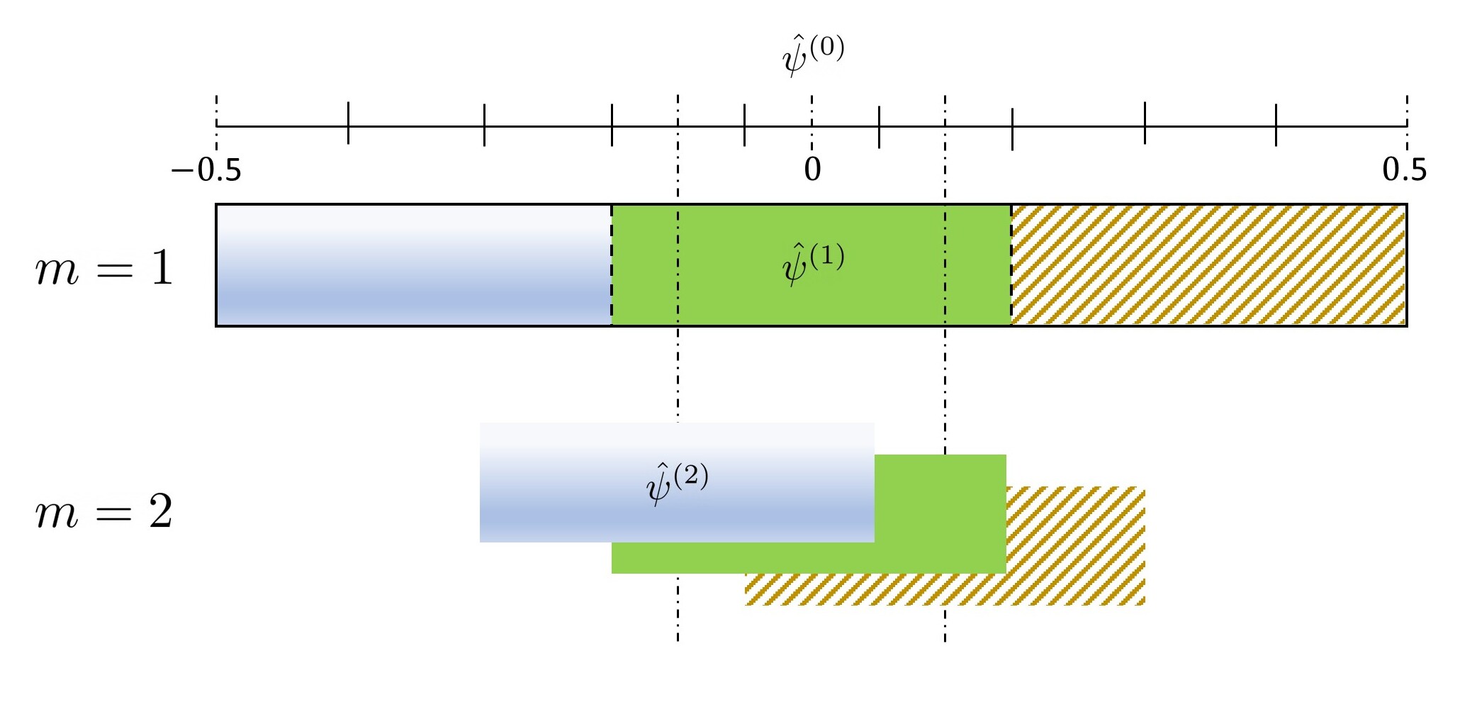
Figure 6: An example of the hierarchical codebook with $(G_{sub},M)=(3,2)$.

IV-B Sequential Search Method With Hierarchical Codebook

We develop a sequential search method using hierarchical codebooks to reduce the computational complexity of the greedy selection in the TS algorithm and enhance the beam resolution in the M-FISTA algorithm. Section IV-B1 introduces the hierarchical codebooks to divide the index selection into multiple levels. Section IV-B2 proposes the sequential search method.

IV-B1 Hierarchical Codebook

In each spatial dimension, we construct a hierarchical codebook to do the index selection on multiple levels. Considering an example of a uniform grid on $[-0.5,0.5)$ of size $G$ along a spatial dimension (same as in (14)) as $\mathcal{G}=\left\{\psi_{i}=\frac{i-\frac{G+1}{2}}{G},\ i=1,\dots,G\right\},$ we divide the index selection of $\mathcal{G}$ into the hierarchical search on $M$ levels, where each level has its sub-codebook of size $G_{sub}$, satisfying $G=G_{sub}^{M}$. We design the $m$-th level sub-codebook as

$$\mathcal{G}^{(m)}(\hat{\psi}^{(m-1)})$$

$$=\Big{\{}\psi_{(m,i)}=\hat{\psi}^{(m-1)}+\frac{i-\frac{G_{sub}+1}{2}}{{G_{sub}}^{m}},\ i=1,\dots,G_{sub}\Big{\}},$$ (29)

where $\hat{\psi}^{(m-1)}$ is the selected codeword from the previous level. The selected codeword is initialized as ${\hat{\psi}^{(0)}=0}$. In the first level ($m\!=\!1$), the index search is implemented with the resolution $G_{sub}^{-1}$. In the subsequent levels ($m\!>\!1$), the index search is done with a finer resolution $G_{sub}^{-m}$ centered around the previously selected $\hat{\psi}^{(m-1)}$. Hence, the total number of codewords to be searched is reduced from $G_{sub}^{M}$ to $MG_{sub}$. In Fig. 6, an example of the hierarchical codebook with $(G_{sub},M)\!=\!(3,2)$ is illustrated. A codebook of size $G\!=\!9$ is divided into $M\!=\!2$ levels, where each level has its sub-codebook with $G_{sub}\!=\!3$. Due to the narrow beam of massive MIMO, $G_{sub}$ should be selected to guarantee the beam coverage of $\mathcal{G}^{(1)}$ on all possible spatial angles.

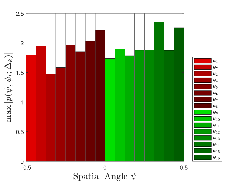
(a)

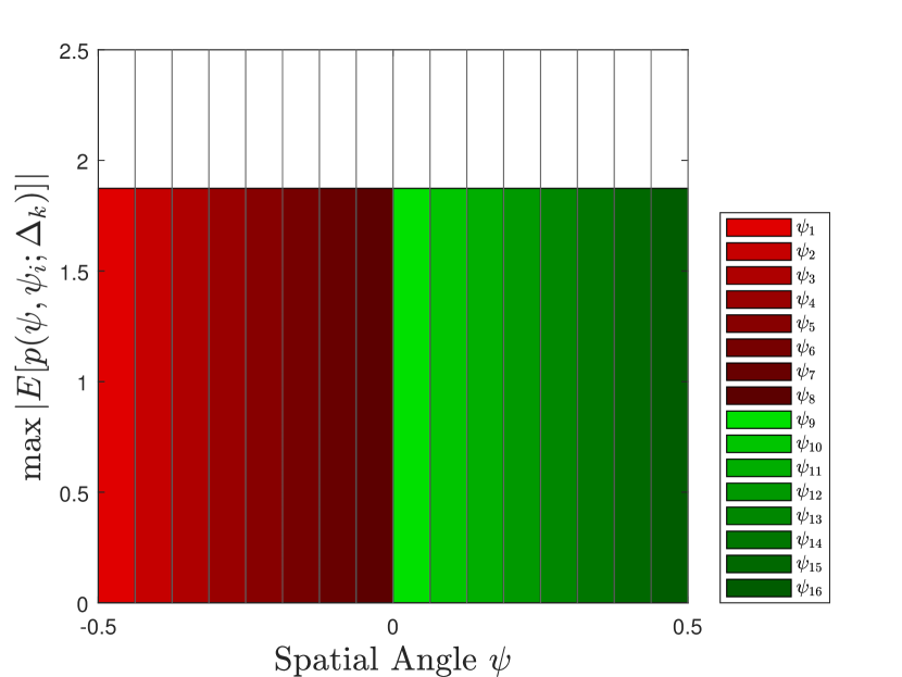
(b)

Figure 7: (a) Beamforming gain $\max_{\psi}\lvert p(\psi,\psi_{i};\Delta_{k})\rvert$ of the effective dictionary vector with $\psi_{i}\in\mathcal{G}^{(1)}$, given $G_{sub}=N=16$, $Q=30$, $B=8$ GHz, $f_{c}=142$ GHz, $k=50$ among $K_{o}=128$ subcarriers. (b) Expected beamforming gain $\max_{\psi}\lvert\mathbb{E}[p(\psi,\psi_{i};\Delta_{k})]\rvert$.

$$\hat{\psi}_{A}^{(m)}=\arg\max_{\psi\in\mathcal{G}_{hT}^{(m)}(\hat{\psi}_{A}^{(m-1)})}\sum\nolimits_{k\in\mathcal{P}}\lvert\mathbf{u}_{k}(\psi,\hat{\psi}_{B}^{(m-1)},\hat{\psi}_{C}^{(m-1)},\hat{\psi}_{D}^{(m-1)})^{H}\mathbf{r}_{k}\rvert^{2},$$ (33)

$$\hat{\psi}_{B}^{(m)}=\arg\max_{\psi\in\mathcal{G}_{vT}^{(m)}(\hat{\psi}_{B}^{(m-1)})}\sum\nolimits_{k\in\mathcal{P}}\lvert\mathbf{u}_{k}(\hat{\psi}_{A}^{(m)},\psi,\hat{\psi}_{C}^{(m-1)},\hat{\psi}_{D}^{(m-1)})^{H}\mathbf{r}_{k}\rvert^{2},$$ (34)

$$\hat{\psi}_{C}^{(m)}=\arg\max_{\psi\in\mathcal{G}_{hR}^{(m)}(\hat{\psi}_{C}^{(m-1)})}\sum\nolimits_{k\in\mathcal{P}}\lvert\mathbf{u}_{k}(\hat{\psi}_{A}^{(m)},\hat{\psi}_{B}^{(m)},\psi,\hat{\psi}_{D}^{(m-1)})^{H}\mathbf{r}_{k}\rvert^{2},$$ (35)

$$\hat{\psi}_{D}^{(m)}=\arg\max_{\psi\in\mathcal{G}_{vR}^{(m)}(\hat{\psi}_{D}^{(m-1)})}\sum\nolimits_{k\in\mathcal{P}}\lvert\mathbf{u}_{k}(\hat{\psi}_{A}^{(m)},\hat{\psi}_{B}^{(m)},\hat{\psi}_{C}^{(m)},\psi)^{H}\mathbf{r}_{k}\rvert^{2},$$ (36)

To choose $G_{sub}$, we analyze the beamwidth of the effective dictionary vector in (18). For ease of exposition, we consider the effective dictionary vector along a spatial dimension as $\mathbf{W}_{k}^{H}\mathbf{a}_{N}(\psi;\Delta_{k})$, where $\mathbf{W}_{k}\!\in\!\mathbb{C}^{N\times Q}$ is the measurement matrix and $\mathbf{a}_{N}(\psi;\Delta_{k})\!\in\!\mathbb{C}^{N\times 1}$ is the array response vector (as in (7)). The beamforming pattern of $\mathbf{W}_{k}^{H}\mathbf{a}_{N}(\psi_{i};\Delta_{k})$, $\psi_{i}\!\in\!\mathcal{G}^{(1)}$ is defined as

$$p(\psi,\psi_{i};\Delta_{k})=\left(\mathbf{W}_{k}^{H}\mathbf{a}_{N}(\psi;\Delta_{k})\right)^{H}\mathbf{W}_{k}^{H}\mathbf{a}_{N}(\psi_{i};\Delta_{k}).$$ (30)

Note that we adopt the random beamforming method for the channel training, i.e., $\mathbf{W}_{k}{(n,q)}=\frac{e^{j\eta_{n,q}}}{\sqrt{N}}$, $\eta_{n,q}\sim\mathcal{U}(0,2\pi)$. The expected beamforming pattern of $\mathbf{W}_{k}^{H}\mathbf{a}_{N}(\psi;\Delta_{k})$ is $\mathbb{E}[p(\psi,\psi_{i};\Delta_{k})]=\frac{Q}{N}\mathbf{a}_{N}(\psi;\Delta_{k})^{H}\mathbf{a}_{N}(\psi_{i};\Delta_{k})$, demonstrating that the expected beamwidth of $\mathbf{W}_{k}^{H}\mathbf{a}_{N}(\psi;\Delta_{k})$ is the same as the beamwidth of $\mathbf{a}_{N}(\psi_{i};\Delta_{k})$, represented by the Half Power Beamwidth (HPBW) ${=0.5\times\textrm{First Null Beamwidth (FNBW)}}$ [48]. We derive $\textrm{FNBW}=\frac{2}{N(1+\Delta_{k}/f_{c})}$ by analyzing the beamforming pattern, so the beamwidth of $\mathbf{a}_{N}(\psi_{i};\Delta_{k})$ is $\textrm{HPBW}\!=\!\frac{1}{N(1+\Delta_{k}/f_{c})}\!\approx\!\frac{1}{N}$. To guarantee the beam coverage of $\mathcal{G}^{(1)}$ on all spatial angles, the resolution ${G_{sub}^{-1}}$ is required to be at least finer than the beamwidth ${N}^{-1}$, so we choose $G_{sub}\!\geq\!N$. In Fig. 7a, we show the beamforming gain of $\mathbf{W}_{k}^{H}\mathbf{a}_{N}(\psi_{i};\Delta_{k})$ with $\psi_{i}\!\in\!\mathcal{G}^{(1)}$, given $N\!=\!G_{sub}\!=\!16$, $Q\!=\!30$, $B\!=\!8$GHz, $f_{c}\!=\!142$GHz, and $k\!=\!50$ among $K_{o}\!=\!128$ subcarriers. The expected beamforming gain is shown in Fig. 7b.

IV-B2 Sequential Search Method

With the extended virtual representation of the MIMO channel in Section II-D, the grid sizes $(G_{hr},G_{vr},G_{ht},G_{vt})$ should be chosen sufficiently large to minimize the grid-mismatch errors between the spatial AOAs/AODs and their quantized values. For the TS algorithm (Algorithm 1), however, the greedy selection (line 13) searches over four different grids $(\mathcal{G}_{hT},\mathcal{G}_{vT},\mathcal{G}_{hR},\mathcal{G}_{vR})$ jointly, which can be reformulated into the problem as

$$\arg\max_{\begin{subarray}{c}(\psi_{A},\psi_{B},\psi_{C},\psi_{D})\\ \in\mathcal{G}_{hT}\times\mathcal{G}_{vT}\times\mathcal{G}_{hR}\times\mathcal{G}_{vR}\end{subarray}}\sum\nolimits_{k\in\mathcal{P}}\lvert\mathbf{u}_{k}(\psi_{A},\psi_{B},\psi_{C},\psi_{D})^{H}\mathbf{r}_{k}\rvert^{2},$$ (31)

where the equivalent dictionary vector is defined as

$$\mathbf{u}_{k} (\psi_{A},\psi_{B},\psi_{C},\psi_{D})$$

$$= \left((\mathbf{a}_{N_{ht}}(\psi_{A};\Delta_{k})\otimes\mathbf{a}_{N_{vt}}(\psi_{B};\Delta_{k}))^{H}\mathbf{X}_{k}\right)^{\top}$$

$$\otimes\left((\mathbf{a}_{N_{hr}}(\psi_{C};\Delta_{k})\otimes\mathbf{a}_{N_{vr}}(\psi_{D};\Delta_{k}))^{H}\mathbf{W}_{k}\right)^{H}.$$

The problem (31) is computationally prohibitive for large grid sizes, due to the exhaustive search over $\{i_{hr},i_{vr},i_{ht},i_{vt}\}\in[1,G_{hr}]\times[1,G_{vr}]\times[1,G_{ht}]\times[1,G_{vt}]$. To address the issue, a sequential search method using hierarchical codebooks is developed to reduce the computational overhead of the greedy selection, detailed as below. First, the problem (32) is solved by searching over the index set $\mathcal{G}_{hT}^{(1)}\times\mathcal{G}_{vT}^{(1)}\times\mathcal{G}_{hR}^{(1)}\times$ $\mathcal{G}_{vR}^{(1)}$ to maximize the objective function, where $\mathcal{G}_{hT}^{(1)}$, $\mathcal{G}_{vT}^{(1)}$, $\mathcal{G}_{hR}^{(1)}$, $\mathcal{G}_{vR}^{(1)}$ are the first-level hierarchical codebooks of $\mathcal{G}_{hT}$, $\mathcal{G}_{vT}$, $\mathcal{G}_{hR}$, $\mathcal{G}_{vR}$, respectively.

$$(\hat{\psi}_{A}^{(1)},\hat{\psi}_{B}^{(1)},\hat{\psi}_{C}^{(1)},\hat{\psi}_{D}^{(1)})=$$

$$\arg\max_{\begin{subarray}{c}(\psi_{A},\psi_{B},\psi_{C},\psi_{D})\\ \in\mathcal{G}_{hT}^{(1)}\times\mathcal{G}_{vT}^{(1)}\times\mathcal{G}_{hR}^{(1)}\times\mathcal{G}_{vR}^{(1)}\end{subarray}}\sum\nolimits_{k\in\mathcal{P}}\lvert\mathbf{u}_{k}(\psi_{A},\psi_{B},\psi_{C},\psi_{D})^{H}\mathbf{r}_{k}\rvert^{2};$$ (32)

We assume the hierarchical codebooks are constructed with the same grid size $G_{sub}$. For the distinct spatial dimensions, $G_{sub}$ can be selected as a different value based on the desired resolution. Next, we sequentially solve the one-dimensional search problems using the hierarchical codebook, starting with the search on the horizontal spatial AODs (33), the vertical spatial AODs (34), the horizontal spatial AOAs (35), and then the vertical spatial AOAs (36), for the level $m=2,\dots,M$. With the sequential search method, we reduce the number of the index sets to be searched from ${G_{ht}G_{vt}G_{hr}G_{vr}=G_{sub}^{4M}}$ to ${G_{sub}^{4}+4(M-1)G_{sub}}$.

For the M-FISTA algorithm (Algorithm 2), instead of reducing the complexity, the sequential search method enhances the resolution of the estimated channel support. M-FISTA first estimates the channel with the low-resolution codebook (line 1-10) inducing the grid-mismatch errors. To address such issue, we apply the sequential search method using the codebook as described in (33)-(36) to estimate the channel support in an enhanced beam resolution (line 11-21).

IV-C Computational Complexity

We recall that TS is done in two stages, MMV-LS and MMV-CS. The complexity of MMV-LS is dominated by the subset selection and its pseudo-inverse operation, searching over the combinations of $\{i_{r},i_{t}\}\in\hat{\Omega}^{pr}$, with complexity $\mathcal{O}\Big{(}\lvert\hat{\Omega}^{pr}\rvert K_{p}(L_{cm})^{3}\Big{)}$ [58]. The complexity of MMV-CS is dictated by the greedy selection, searching over all combinations of $\{g_{r},g_{t}\}\in\mathcal{J}$, with complexity $\mathcal{O}\Big{(}G_{r}G_{t}K_{p}Q_{p}T_{p}\hat{L}\Big{)}$, where $\hat{L}$ is the number of estimated paths. The TS algorithm requires traversing over all candidate AOA-AOD pairs for the greedy beam selection in MMV-CS, which leads to a prohibitive average execution time. It can be reduced by parallel processing because the correlation with the signal of each AOA-AOD pair could be calculated separately, called TS with parallel processing. The proposed sequential search method greatly alleviates the overhead of the greedy selection, leading to the complexity $\mathcal{O}\Big{(}({G_{sub}^{4}}+4(M-1)G_{sub})K_{p}Q_{p}T_{p}\hat{L}\Big{)}$. For M-FISTA, the complexity is dominated by the gradient calculation $\nabla f$. Thanks to the block diagonal structure of $\mathbf{\Phi}_{A}$ and $\mathbf{\Phi}_{B}$, the gradient $\nabla f$ can be calculated on each subcarrier separately, which reduces the complexity from $\mathcal{O}\Big{(}K_{p}^{3}G_{r}^{2}G_{t}^{2}Q_{p}T_{p}\Big{)}$ to $\mathcal{O}\Big{(}K_{p}Q_{p}T_{p}\lvert\Gamma\rvert\lvert\Gamma^{c}\rvert\Big{)}$, where $\Gamma$ is the previous channel support. Note that M-FISTA is not suitable to operate with parallel processing since it applies the proximal gradient descent method. For the channel refinement algorithm, the complexity is dominated by the least squares operations (25). Assuming $L^{\prime}$ estimated paths, the update of $\mathbf{q}_{k}$ requires the pseudo-inverse operations on pilot subcarriers with complexity $\mathcal{O}\left(K_{p}(L^{\prime})^{3}\right)$. With the configuration as in TABLE I, we evaluate the complexity in terms of the average execution time: $30.12$s for TS, $7.12$s for TS with parallel processing, $21.7$s for M-FISTA, $16.1$s for M-FISTA without previous support, as opposed to $34.2$s for GSOMP (state-of-the-art). Note that TS with parallel processing starts a pool of $12$ workers in MATLAB for the greedy beam selection, which reduces the average execution time by $76$% in our configuration.

TABLE I: Common Simulation Parameters [3, 4]

Parameter	Symbol	Value
Carrier frequency	$f_{c}$	$142$ GHz
Bandwidth	$B$	$8$ GHz
Total subcarriers	$K_{o}$	$1024$
Channel paths	$(L,L_{cm})$	$(4,3)$
Ref. path coefficient	$\alpha_{\ell}^{\prime}$	$\mathcal{CN}(0,\sigma_{\alpha}^{2})$
Polar AOA/AOD	$\theta_{pr}/\theta_{pt}$	$\mathcal{U}(-\pi/2,\pi/2)$
Azimuth AOA/AOD	$\theta_{ar}/\theta_{at}$	$\mathcal{U}(-\pi,\pi)$
Tx antenna (UPA)	$N_{t}\ (N_{vt},N_{ht})$	$16\ (4,4)$
Rx antenna (UPA)	$N_{r}\ (N_{vr},N_{hr})$	$256\ (16,16)$
Tx/Rx sub-codebook	$(G_{sub,t},G_{sub,r})$	$(4,16)$
Pilot subcarriers	$K_{p}$	$10$
Training parameters	$(Q_{p},T_{p})$	$(25,25)$
Subframe/Frame duration	$\delta_{s}/T_{frame}$	$10\mu\textrm{s}/10\textrm{ms}$

V Numerical Results

We evaluate the performance of the proposed channel estimation in time-varying MIMO-OFDM, and the numerical parameters are listed in Table I. We consider the multipath channel having delays $\tau_{\ell}\sim\mathcal{U}(45,55)\textrm{ns}$ with the delay spread $D_{s}=10\textrm{ns}$ [4]. This yields a coherence bandwidth $B_{c}=\frac{1}{2D_{s}}=50\textrm{MHz}$ [51] and the minimum number of subcarriers $\frac{B}{B_{c}}=160$. We consider the total number of subcarriers as $K_{o}=1024$. The receive and transmit array response matrices $\mathbf{A}_{R,k}$, $\mathbf{A}_{T,k}$ are constructed as in (15) (16), with the uniform grid $\mathcal{G}_{R}\!=\!\mathcal{G}_{hR}\times\mathcal{G}_{vR}$ of size $G_{r}\!=\!G_{hr}G_{vr}$ and the uniform grid $\mathcal{G}_{T}\!=\!\mathcal{G}_{hT}\times\mathcal{G}_{vT}$ of size $G_{t}\!=\!G_{ht}G_{vt}$, respectively. The sequential search method with hierarchical codebooks as described in Section IV-B is applied. We consider a transmit hierarchical codebook with $(G_{sub,t},M)$ for the uniform grids $\mathcal{G}_{hT}$, $\mathcal{G}_{vT}$, i.e., $G_{ht}\!=\!G_{vt}\!=\!G_{sub,t}^{M}$. Similarly, a receive hierarchical codebook with $(G_{sub,r},M)$ is considered for the uniform grids $\mathcal{G}_{hR}$, $\mathcal{G}_{vR}$, i.e., $G_{hr}\!=\!G_{vr}\!=\!G_{sub,r}^{M}$. The receiving signal-to-noise ratio is defined as $\textrm{SNR}\!=\!\mathbb{E}\left[\frac{\sum_{k}\lVert\mathbf{W}_{k}^{H}\mathbf{H}_{k}\mathbf{X}_{k}\rVert_{F}^{2}}{\sum_{k}\mathbb{E}\left[\lVert\mathbf{\tilde{V}}_{k}\rVert_{F}^{2}\mid\mathbf{W}_{k},\mathbf{X}_{k},\mathbf{H}_{k},\forall k\right]}\right]$, where $\mathbf{W}_{k}$, $\mathbf{X}_{k}$, $\mathbf{H}_{k}$, and $\mathbf{\tilde{V}}_{k}$ are the measurement, pilot, channel, and combined noise matrices, respectively, as in (18).

We compare the proposed TS and M-FISTA channel estimation (with the ”estimated” previous channel support) with the estimation schemes listed as follows:

• GSOMP [11]: Apply the SOMP to estimate the AOAs/AODs and channel gains (with frequency-dependent dictionary matrices) using common support across the pilot subcarriers. GSOMP considers the dual-wideband effect.

• DGMP [22]: Apply the distributed CS to estimate the AOAs/AODs and channel gains (with frequency-flat dictionary matrices) using the structured sparsity and the grid mismatch pursuit strategy. We extend this design to the UPA case for comparison. DGMP considers the frequency-wideband effect but neglects the spatial-wideband effect.

• Genie-aided LS: The LS estimator is applied with the current channel support. This is considered a performance bound.

We also evaluate M-FISTA without previous channel support, called M-FISTA w/o prev support, which sets $\Gamma=\emptyset$ and ignores the term $\lambda_{1}\lVert\mathbf{\tilde{z}}^{LS}\rVert_{2,1}$ in (23). Note that we consider the number of training measurements with $(Q_{p},T_{p})=(25,25)$ (partial training of $15.3\%N_{r}N_{t}$ beams), while the work [11] evaluates the GSOMP estimator under the partial training of $80\%N_{r}N_{t}$ beams, which is much larger than our considered setting. In addition, the support tracking-based approaches needs to do the initial channel estimation (i.e., MMV-CS for TS or M-FISTA w/o prev support for M-FISTA) if the residual signal power is larger than a predefined threshold. In our simulation, the predefined threshold is chosen such that the number of frames of the initial channel estimation (i.e., $\hat{\Omega}^{pr}=\emptyset$) is less than $10\%$ of all frames. Note that the frames implementing the initial channel estimation are counted in the performance evaluation.

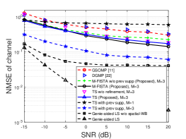
Figure 8: The NMSE versus the SNR.

To evaluate the channel estimation accuracy, we define the normalized mean squared error (NMSE) of the estimated channel as

$$\textrm{NMSE}=\frac{\sum_{k\in\mathcal{P}}\lVert\mathbf{H}_{k}-\mathbf{\hat{H}}_{k}\rVert_{F}^{2}}{\sum_{k\in\mathcal{P}}\lVert\mathbf{H}_{k}\rVert_{F}^{2}}.$$ (37)

In Fig. 8, we evaluate the NMSE of channel versus the SNR. Genie-aided LS attains $\text{NMSE}\!=\!1.5\times 10^{-2}$ above $\text{SNR}\!=\!-5$dB, which provides a lower bound for the NMSE. Genie-aided LS w/o spatial-WB applies the LS estimator with the correct AOAs/AODs, ignoring the spatial-wideband effect in the channel reconstruction. Even with the correct AOAs/AODs estimation, it attains only $\text{NMSE}\!=\!4\times 10^{-2}$ when $\text{SNR}\!\geq\!0$dB due to the spatial-wideband effect. To determine a suitable number of levels $M$ of the hierarchical codebook, we evaluate TS with the “correct” previous channel support (called TS with prev support) scheme with different $M$. For $M\!=\!1$, TS with prev support attains $\text{NMSE}\!=\!0.6$ with $\textrm{SNR}\!=\!10$dB. In the same configuration, the NMSE improves with a larger $M$, attaining $0.07$ for $M\!=\!3$. We observe that there is only minor improvement as we increase the number of levels from $M=3$ to $M\!=\!4$. Thus, $M\!=\!3$ is chosen for the following experiments. Given an $\textrm{SNR}\!=\!20$dB, the proposed TS attains $\textrm{NMSE}=0.17$, as opposed to $0.06$ for TS with prev support, $0.29$ for GSOMP, and $0.32$ for DGMP. TS is inferior to TS with prev support due to the potential errors in the estimated previous channel support because of the algorithm’s reliance on accurate past support estimation, which is difficult at low SNR. With $\textrm{SNR}\!=\!-10$dB, TS attains $\textrm{NMSE}\!=\!0.52$ while the TS w/o refinement only has $\textrm{NMSE}\!=\!0.7$. It shows that given the same estimated AOAs/AODs of the channel paths, the channel refinement algorithm improves the estimation accuracy in the low SNR region. In addition, with $\textrm{SNR}\!=\!20$dB, the proposed M-FISTA attains $\textrm{NMSE}\!=\!0.14$, as opposed to $\textrm{NMSE}\!=\!0.22$ for M-FISTA w/o previous support. We observe that M-FISTA has a better NMSE performance than M-FISTA w/o previous support at the high SNR region because the previous channel support can be estimated more accurately, which is beneficial to the LS-CS framework. When $\textrm{SNR}\!<\!0$dB, M-FISTA attains a similar NMSE to M-FISTA w/o prev support.

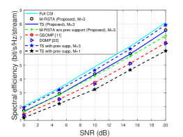
Figure 9: Spectral efficiency versus the SNR, with $N_{s}=4$.

Next, we evaluate the spectral efficiency (SE). The rate expression maximized by Gaussian signaling [10] over the channel is expressed as

$$R\!=\!\sum_{k=1}^{K_{o}}\!\frac{B}{K_{o}}\log_{2}\textrm{det}\left(\mathbf{I}_{N_{s}}+\frac{P_{t}}{N_{s}}\mathbf{R}_{\hat{\mathbf{v}}_{k}}^{-1}\mathbf{\hat{W}}_{k}^{H}\mathbf{H}_{k}\mathbf{\hat{F}}_{k}\mathbf{\hat{F}}_{k}^{H}\mathbf{H}_{k}^{H}\mathbf{\hat{W}}_{k}\right),$$ (38)

where $P_{t}$ is the average transmit power for each transmission. The number of data streams is assumed as $N_{s}=4$. The unconstrained combiner $\mathbf{\hat{W}}_{k}$ (or the precoder $\mathbf{\hat{F}}_{k}$) is derived by the directions of the eigenvectors of $\mathbf{\hat{H}}_{k}\mathbf{\hat{H}}_{k}^{H}$ (or $\mathbf{\hat{H}}_{k}^{H}\mathbf{\hat{H}}_{k}$). The post-processing noise covariance matrix is $\mathbf{R}_{\hat{\mathbf{v}}_{k}}=\mathbb{E}[\hat{\mathbf{v}}_{k}\hat{\mathbf{v}}_{k}^{H}]$, where $\hat{\mathbf{v}}_{k}=\mathbf{\hat{W}}_{k}^{H}\mathbf{v}$ with the additive complex Gaussian noise $\mathbf{v}$. The fraction of time for the pilot transmission is $\iota\!=\!\frac{T_{train}}{T_{frame}}$, where the duration of $T_{train}\!=\!T_{p}\delta_{s}$ on the $K_{p}$ pilot subcarriers is the resulting training overhead. The data transmission is allowed on the entire bandwidth at the transmission time, and also on the bandwidth other than the pilot subcarriers at the training time. We denote the rate on the training time as $R_{train}$, which is constructed as in (38) without the pilot subcarriers. Thus, the SE is defined as $\frac{\iota R_{train}+(1-\iota)R}{BN_{s}}$ (bit/s/Hz/stream), which includes the loss due to the training overhead. In Fig. 9, we evaluate the SE versus the SNR. Full CSI attains the largest SE because its $\mathbf{\hat{W}}_{k}$ and $\mathbf{\hat{F}}_{k}$ are derived from the perfect CSI. TS with prev support scheme attains a better SE with a larger number of levels, consistent with the NMSE evaluation. For $\textrm{SNR}\!=\!20$dB, the SE of M-FISTA and TS both attain $7.6$ bit/s/Hz/stream, while the SE of GSOMP and DGMP are $6.63$bit/s/Hz/stream and $6.58$bit/s/Hz/stream, respectively. As opposed to TS with prev support, the SE loss of TS is around $0.42$bit/s/Hz/stream, originating from the potential errors in the estimated previous channel support. Even for the case with no previous channel support, our proposed M-FISTA w/o prev support attains $7.1$bit/s/Hz/stream, which also outperforms the state-of-the-art (GSOMP) by $0.5$bit/s/Hz/stream.

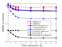
Figure 10: The NMSE versus the number of pilot subcarriers $K_{p}$, with $\textrm{SNR}=-10$dB.

In Fig. 10, we evaluate the NMSE versus the number of pilot subcarriers $K_{p}$, with $\textrm{SNR}=-10$dB. For $K_{p}=1$, we perform LS estimation to reconstruct the channel for the schemes with refinement since there are no multiple subcarriers to do the channel refinement algorithm. With $K_{p}=1$, we have $\textrm{NMSE}=1.1$ for both the TS and M-FISTA, as opposed to $\textrm{NMSE}=0.04$ for Genie-aided LS, $\textrm{NMSE}=0.8$ for TS with prev support, $\textrm{NMSE}=1.38$ for GSOMP, and $\textrm{NMSE}=1.23$ for DGMP. As we increase to $K_{p}\!=\!5$, we observe that the NMSE of TS and M-FISTA significantly improve to $\textrm{NMSE}\!=\!0.56$ and $\textrm{NMSE}\!=\!0.61$, respectively. The improvement comes from the MMV using the common channel support across subcarriers. Also, the channel refinement algorithm provides a more accurate estimation, especially in the low SNR region. Note that the NMSE of M-FISTA w/o prev support is omitted in Fig. 10 since it is similar to the one of M-FISTA in the low SNR region. We observe that Genie-aided LS with refinement attains $\textrm{NMSE}\!=\!0.018$ when $K_{p}\!=\!5$, as opposed to Genie-aided LS attains $\textrm{NMSE}\!=\!0.04$. The improvement arises from fitting the reference path coefficients and time delays across subcarriers. For $K_{p}>5$, all approaches have fairly minor improvement with additional pilot subcarriers.

In Fig. 11, with $\textrm{SNR}=20$dB, we evaluate the NMSE of the estimated channel versus the measurement ratio $M_{p}\!=\!\frac{N_{p}}{N_{r}N_{t}}$, where $N_{p}$ is the number of training measurements. Given $N_{p}$ measurements, we assume the training parameters as $Q_{p}\!=\!T_{p}\!=\!\sqrt{N_{p}}$. The NMSE of channel decreases with more training measurements. TS and M-FISTA both attain $\textrm{NMSE}=0.7$ with $M_{p}=3.5\%$ ($Q_{p}\!=\!T_{p}\!=\!12$), as opposed to GSOMP and DGMP achieves $\textrm{NMSE}\!=\!0.90$ and $\textrm{NMSE}\!=\!0.88$ in the same configuration. As we increase the training measurements to $M_{p}\!=\!15.3\%$ ($Q_{p}\!=\!T_{p}\!=\!25$), the NMSE performance improves ($\textrm{NMSE}\!=\!0.17$ for TS, $\textrm{NMSE}\!=\!0.14$ for M-FISTA, $\textrm{NMSE}\!=\!0.23$ for M-FISTA w/o prev support, $\textrm{NMSE}\!=\!0.32$ for DGMP, and $\textrm{NMSE}\!=\!0.29$ for GSOMP), which shows the advantage of our MMV-LS-CS channel training.

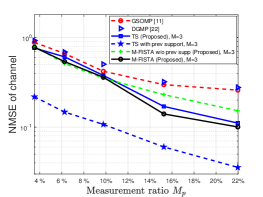
Figure 11: The NMSE versus the measurement ratio $M_{p}=Q_{p}T_{p}/N_{r}N_{t}$, with $\textrm{SNR}=20$dB.

In Fig. 12, we evaluate the NMSE of the estimated channel versus the bandwidth, with $\textrm{SNR}\!=\!20$dB. As the bandwidth increases from $0.7$ to $8$ GHz, the NMSE of channel increases by around $0.005$ for TS and $0.006$ for M-FISTA, as opposed to $0.03$ for GSOMP and $0.04$ for GSOMP. The TS, M-FISTA, and GSOMP algorithm are not sensitive to the change of bandwidths owing to the frequency-dependent dictionary matrices. In this configuration, the Genie-aided LS w/o spatial-WB scheme deteriorates from $\textrm{NMSE}\!=\!2.7\times 10^{-3}$ to $\textrm{NMSE}\!=\!4\times 10^{-2}$ because the dual-wideband effect becomes more severe with a larger bandwidth. We observe that the NMSE of channel increases even with the accurate AOAs/AODs estimation if the spatial-wideband effect is neglected, which shows the necessity of using the frequency-dependent dictionary matrices.

VI Conclusion

We proposed a CS channel training for time-varying sub-THz dual-wideband MIMO-OFDM systems. We constructed the frequency-dependent array response matrices to preserve the common channel support among subcarriers and enabled the MMV channel recovery. For slowly-varying channels, we employed the previous channel support to develop an MMV-LS-CS framework, and proposed two channel estimation algorithms (TS and M-FISTA). The TS algorithm adopts a two-stage procedure to do the MMV-CS on the MMV-LS residual signal. The M-FISTA algorithm solved a joint MMV-LS-CS using the framework of FISTA. We proposed a channel refinement algorithm to reconstruct the channel by estimating the time delays and path coefficients jointly on the subcarriers, leveraging the spreading loss structure. To reduce the computational complexity and enhance the beam resolution, we proposed a sequential search method using hierarchical codebooks. Numerical results showed that the TS and M-FISTA algorithms provide improved estimation accuracy and SE over the state-of-the-art techniques.

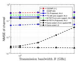
Figure 12: The NMSE versus the transmission bandwidth $B$, with $\textrm{SNR}=20$dB.

Tzu-Hsuan Chou (Member, IEEE) received the B.S. degree in electrical engineering and the M.S. degree in electrical and control engineering from National Chiao Tung University, Hsinchu, Taiwan, in 2011 and 2013, respectively, and the Ph.D. degree in electrical and computer engineering from Purdue University, West Lafayette, IN, USA, in 2022. He is currently a Senior Engineer with Qualcomm Inc., San Diego, CA, USA. From 2014 to 2017, he was a Software Engineer with MediaTek, Hsinchu, Taiwan. His research interests include massive MIMO, wireless communications, compressed sensing, and tensor decomposition for signal processing.

Nicolò Michelusi (Senior Member, IEEE) received the B.Sc. (with honors), M.Sc. (with honors), and Ph.D. degrees from the University of Padova, Italy, in 2006, 2009, and 2013, respectively, and the M.Sc. degree in telecommunications engineering from the Technical University of Denmark, Denmark, in 2009, as part of the T.I.M.E. double degree program. From 2013 to 2015, he was a Postdoctoral Research Fellow with the Ming-Hsieh Department of Electrical Engineering, University of Southern California, Los Angeles, CA, USA, and from 2016 to 2020, he was an Assistant Professor with the School of Electrical and Computer Engineering, Purdue University, West Lafayette, IN, USA. He is currently an Assistant Professor with the School of Electrical, Computer and Energy Engineering, Arizona State University, Tempe, AZ, USA. His research interests include 5G wireless networks, millimeter-wave communications, stochastic optimization, distributed optimization, and federated learning over wireless systems. He served as Associate Editor for the IEEE TRANSACTIONS ON WIRELESS COMMUNICATIONS from 2016 to 2021, and currently serves as Editor for the IEEE TRANSACTIONS ON COMMUNICATIONS. He was the Co-Chair for the Distributed Machine Learning and Fog Network workshop at the IEEE INFOCOM 2021, the Wireless Communications Symposium at the IEEE Globecom 2020, the IoT, M2M, Sensor Networks, and Ad-Hoc Networking track at the IEEE VTC 2020, and the Cognitive Computing and Networking symposium at the ICNC 2018. He is the Technical Area Chair for the Communication Systems track at Asilomar 2023. He received the NSF CAREER award in 2021 and the 2022 Early Achievement Award of the IEEE Communications Society - Communication Theory Technical Committee (CTTC).

David J. Love (Fellow, IEEE) received the B.S. (with highest honors), M.S.E., and Ph.D. degrees in electrical engineering from the University of Texas at Austin in 2000, 2002, and 2004, respectively. Since 2004, he has been with the Elmore Family School of Electrical and Computer Engineering at Purdue University, where he is now the Nick Trbovich Professor of Electrical and Computer Engineering. He served as a Senior Editor for IEEE Signal Processing Magazine, Editor for the IEEE Transactions on Communications, Associate Editor for the IEEE Transactions on Signal Processing, and guest editor for special issues of the IEEE Journal on Selected Areas in Communications and the EURASIP Journal on Wireless Communications and Networking. He was a member of the Executive Committee for the National Spectrum Consortium. He holds 32 issued U.S. patents. His research interests are in the design and analysis of broadband wireless communication systems, beyond-5G wireless systems, multiple-input multiple-output (MIMO) communications, millimeter wave wireless, software defined radios and wireless networks, coding theory, and MIMO array processing. Dr. Love is a Fellow of the American Association for the Advancement of Science (AAAS) and was named a Thomson Reuters Highly Cited Researcher (2014 and 2015). Along with his co-authors, he won best paper awards from the IEEE Communications Society (2016 Stephen O. Rice Prize and 2020 Fred W. Ellersick Prize), the IEEE Signal Processing Society (2015 IEEE Signal Processing Society Best Paper Award), and the IEEE Vehicular Technology Society (2010 Jack Neubauer Memorial Award).

James V. Krogmeier (Senior Member, IEEE) received the B.S.E.E. degree from the University of Colorado Boulder, Boulder, CO, USA, and the M.S. and Ph.D. degrees from the University of Illinois at Urbana-Champaign, Champaign, IL, USA. He has industry experience in telecommunications and is a Founding Member of two software startup companies. He is currently a Professor of electrical and computer engineering with Purdue University, West Lafayette, IN, USA. He has authored or coauthored many technical papers in refereed journals and conference proceedings of the IEEE, the ASABE, and the Transportation Research Board, and is a Co-Inventor of five U.S. patents. His research interests include the applications of statistical signal and image processing in agriculture, intelligent transportation systems, sensor networking, and wireless communications. His research has been funded by the USDA-NIFA, the NSF, the DARPA, the Indiana Department of Transportation, the Federal Highway Administration, and industry. He was on a number of IEEE technical program committees and an Associate Editor for several IEEE journals.

References

- [1] T.-H. Chou, N. Michelusi, D. J. Love, and J. V. Krogmeier, “Wideband Millimeter-Wave Massive MIMO Channel Training via Compressed Sensing,” in Proc. IEEE Glob. Commun. Conf., 2021, pp. 1–6.
- [2] J. G. Andrews, S. Buzzi, W. Choi, S. V. Hanly, A. Lozano, A. C. Soong, and J. C. Zhang, “What will 5G be?” IEEE J. Sel. Areas Commun, vol. 32, no. 6, pp. 1065–1082, Jun. 2014.
- [3] T. S. Rappaport, Y. Xing, O. Kanhere, S. Ju, A. Madanayake, S. Mandal, A. Alkhateeb, and G. C. Trichopoulos, “Wireless Communications and Applications Above 100 GHz: Opportunities and Challenges for 6G and Beyond,” IEEE Access, vol. 7, pp. 78 729–78 757, Apr. 2019.
- [4] Y. Xing, T. S. Rappaport, and A. Ghosh, “Millimeter Wave and sub-THz Indoor Radio Propagation Channel Measurements, Models, and Comparisons in an Office Environment,” IEEE Commun. Lett., pp. 1–1, Oct. 2021.
- [5] S. Ju, Y. Xing, O. Kanhere, and T. S. Rappaport, “Millimeter Wave and Sub-Terahertz Spatial Statistical Channel Model for an Indoor Office Building,” IEEE J. Sel. Areas Commun., vol. 39, no. 6, pp. 1561–1575, Jun. 2021.
- [6] C. Lin and G. Y. Li, “Adaptive Beamforming With Resource Allocation for Distance-Aware Multi-User Indoor Terahertz Communications,” IEEE Trans. Commun., vol. 63, no. 8, pp. 2985–2995, Aug. 2015.
- [7] J. M. Jornet and I. F. Akyildiz, “Channel modeling and capacity analysis for electromagnetic wireless nanonetworks in the terahertz band,” IEEE Trans. Wireless Commun., vol. 10, no. 10, pp. 3211–3221, Oct. 2011.
- [8] R. Piesiewicz, C. Jansen, D. Mittleman, T. Kleine-Ostmann, M. Koch, and T. Kurner, “Scattering Analysis for the Modeling of THz Communication Systems,” IEEE Trans. Antennas Propag., vol. 55, no. 11, pp. 3002–3009, Nov. 2007.
- [9] E. G. Larsson, O. Edfors, F. Tufvesson, and T. L. Marzetta, “Massive MIMO for next generation wireless systems,” IEEE Commun. Mag., vol. 52, no. 2, pp. 186–195, Feb. 2014.
- [10] A. Alkhateeb, O. El Ayach, G. Leus, and R. W. Heath, “Channel Estimation and Hybrid Precoding for Millimeter Wave Cellular Systems,” IEEE J. Sel. Top. Signal Process., vol. 8, no. 5, pp. 831–846, Oct. 2014.
- [11] K. Dovelos, M. Matthaiou, H. Q. Ngo, and B. Bellalta, “Channel Estimation and Hybrid Combining for Wideband Terahertz Massive MIMO Systems,” IEEE J. Sel. Areas Commun., vol. 39, no. 6, pp. 1604–1620, Jun. 2021.
- [12] B. Wang, F. Gao, S. Jin, H. Lin, and G. Y. Li, “Spatial- and frequency-wideband effects in millimeter-wave massive MIMO systems,” IEEE Trans. Signal Process., vol. 66, no. 13, pp. 3393–3406, Jul. 2018.
- [13] B. Wang, M. Jian, F. Gao, G. Y. Li, and H. Lin, “Beam squint and channel estimation for wideband mmWave massive MIMO-OFDM systems,” IEEE Trans. Signal Process., vol. 67, no. 23, pp. 5893–5908, Dec. 2019.
- [14] M. Wang, F. Gao, N. Shlezinger, M. F. Flanagan, and Y. C. Eldar, “A block sparsity based estimator for mmWave massive MIMO channels with beam squint,” IEEE Trans. Signal Process., vol. 68, pp. 49–64, Nov. 2019.
- [15] Y. Lin, S. Jin, M. Matthaiou, and X. You, “Tensor-Based Channel Estimation for Millimeter Wave MIMO-OFDM With Dual-Wideband Effects,” IEEE Trans. Commun., vol. 68, no. 7, pp. 4218–4232, Jul. 2020.
- [16] J. Tan and L. Dai, “Wideband channel estimation for THz massive MIMO,” China Commun., vol. 18, no. 5, pp. 66–80, May 2021.
- [17] Z. Marzi, D. Ramasamy, and U. Madhow, “Compressive Channel Estimation and Tracking for Large Arrays in mm-Wave Picocells,” IEEE J. Sel. Topics Signal Process., vol. 10, no. 3, pp. 514–527, Apr. 2016.
- [18] K. Venugopal, A. Alkhateeb, N. G. Prelcic, and R. W. Heath, “Channel estimation for hybrid architecture-based wideband millimeter wave systems,” IEEE J. Sel. Areas Commun., vol. 35, no. 9, pp. 1996–2009, Sep. 2017.
- [19] Z. Zhou, J. Fang, L. Yang, H. Li, Z. Chen, and R. S. Blum, “Low-Rank Tensor Decomposition-Aided Channel Estimation for Millimeter Wave MIMO-OFDM Systems,” IEEE J. Sel. Areas Commun., vol. 35, no. 7, pp. 1524–1538, Jul. 2017.
- [20] D. C. Araújo, A. L. De Almeida, J. P. Da Costa, and R. T. de Sousa, “Tensor-Based Channel Estimation for Massive MIMO-OFDM Systems,” IEEE Access, vol. 7, pp. 42 133–42 147, Mar. 2019.
- [21] Z. Gao, L. Dai, Z. Wang, and S. Chen, “Spatially Common Sparsity Based Adaptive Channel Estimation and Feedback for FDD Massive MIMO,” IEEE Transactions on Signal Processing, vol. 63, no. 23, pp. 6169–6183, Dec. 2015.
- [22] Z. Gao, C. Hu, L. Dai, and Z. Wang, “Channel estimation for millimeter-wave massive MIMO with hybrid precoding over frequency-selective fading channels,” IEEE Commun. Lett., vol. 20, no. 6, pp. 1259–1262, Apr. 2016.
- [23] J. Choi and R. W. Heath, “Interpolation based transmit beamforming for MIMO-OFDM with limited feedback,” IEEE Trans. Signal Process., vol. 53, no. 11, pp. 4125–4135, Nov. 2005.
- [24] T. Pande, D. J. Love, and J. V. Krogmeier, “A Weighted Least Squares Approach to Precoding With Pilots for MIMO-OFDM,” IEEE Trans. Signal Process., vol. 54, no. 10, pp. 4067–4073, Oct. 2006.
- [25] ——, “Reduced Feedback MIMO-OFDM Precoding and Antenna Selection,” IEEE Trans. Signal Process., vol. 55, no. 5, pp. 2284–2293, May 2007.
- [26] S. L. H. Nguyen, J. Järveläinen, A. Karttunen, K. Haneda, and J. Putkonen, “Comparing radio propagation channels between 28 and 140 GHz bands in a shopping mall,” in Proc. Eur. Conf. Antennas Propag. (EuCAP), Apr. 2018, pp. 1–5.
- [27] T. Nitsche, C. Cordeiro, A. B. Flores, E. W. Knightly, E. Perahia, and J. C. Widmer, “IEEE 802.11 ad: directional 60 GHz communication for multi-Gigabit-per-second Wi-Fi,” IEEE Commun. Mag., vol. 52, no. 12, pp. 132–141, Dec. 2014.
- [28] M. Giordani, M. Polese, A. Roy, D. Castor, and M. Zorzi, “A Tutorial on Beam Management for 3GPP NR at mmWave Frequencies,” IEEE Commun. Surveys Tuts., vol. 21, no. 1, pp. 173–196, Sep. 2018.
- [29] S. Wu, C.-X. Wang, H. Haas, e.-H. M. Aggoune, M. M. Alwakeel, and B. Ai, “A non-stationary wideband channel model for massive MIMO communication systems,” IEEE Trans. Wireless Commun., vol. 14, no. 3, pp. 1434–1446, Mar. 2015.
- [30] Y. Chen and C. Han, “Time-Varying Channel Modeling for Low-Terahertz Urban Vehicle-to-Infrastructure Communications,” in Proc. IEEE Glob. Commun. Conf., 2019, pp. 1–6.
- [31] Y. Han, J. Lee, and D. J. Love, “Compressed Sensing-Aided Downlink Channel Training for FDD Massive MIMO Systems,” IEEE Trans. Commun., vol. 65, no. 7, pp. 2852–2862, Jul. 2017.
- [32] M. Hussain and N. Michelusi, “Energy-Efficient Interactive Beam Alignment for Millimeter-Wave Networks,” IEEE Trans. Wireless Commun., vol. 18, no. 2, pp. 838–851, Feb. 2018.
- [33] M. Hussain, M. Scalabrin, M. Rossi, and N. Michelusi, “Mobility and Blockage-Aware Communications in Millimeter-Wave Vehicular Networks,” IEEE Trans. Veh. Technol., vol. 69, no. 11, pp. 13 072–13 086, Nov. 2020.
- [34] M. Hussain and N. Michelusi, “Learning and Adaptation for Millimeter-Wave Beam Tracking and Training: a Dual Timescale Variational Framework,” IEEE J. Sel. Areas Commun., pp. 1–1, Nov. 2021.
- [35] S. Hur, T. Kim, D. J. Love, J. V. Krogmeier, T. A. Thomas, and A. Ghosh, “Millimeter Wave Beamforming for Wireless Backhaul and Access in Small Cell Networks,” IEEE Trans. Commun., vol. 61, no. 10, pp. 4391–4403, Oct. 2013.
- [36] M. B. Booth, V. Suresh, N. Michelusi, and D. J. Love, “Multi-Armed Bandit Beam Alignment and Tracking for Mobile Millimeter Wave Communications,” IEEE Commun. Lett., vol. 23, no. 7, pp. 1244–1248, Jul. 2019.
- [37] D. J. Love and R. W. Heath, “Equal gain transmission in multiple-input multiple-output wireless systems,” IEEE Trans. Commun., vol. 51, no. 7, pp. 1102–1110, Jul. 2003.
- [38] D. J. Love, R. W. Heath, and T. Strohmer, “Grassmannian beamforming for multiple-input multiple-output wireless systems,” IEEE Trans. Inf. Theory, vol. 49, no. 10, pp. 2735–2747, Oct. 2003.
- [39] D. J. Love, R. W. Heath, V. K. Lau, D. Gesbert, B. D. Rao, and M. Andrews, “An overview of limited feedback in wireless communication systems,” IEEE J. Sel. Areas Commun., vol. 26, no. 8, pp. 1341–1365, Oct. 2008.
- [40] S. G. Larew and D. J. Love, “Adaptive Beam Tracking With the Unscented Kalman Filter for Millimeter Wave Communication,” IEEE Signal Process. Lett., vol. 26, no. 11, pp. 1658–1662, 2019.
- [41] T.-H. Chou, N. Michelusi, D. J. Love, and J. V. Krogmeier, “Fast Position-Aided MIMO Beam Training via Noisy Tensor Completion,” IEEE J. Sel. Top. Signal Process., vol. 15, no. 3, pp. 774–788, Apr. 2021.
- [42] M. Hashemi, C. E. Koksal, and N. B. Shroff, “Out-of-Band Millimeter Wave Beamforming and Communications to Achieve Low Latency and High Energy Efficiency in 5G Systems,” IEEE Trans. Commun., vol. 66, no. 2, pp. 875–888, Feb 2018.
- [43] N. González-Prelcic, R. Méndez-Rial, and R. W. Heath, “Radar aided beam alignment in mmWave V2I communications supporting antenna diversity,” in Proc. Inf. Theory Appl. Workshop, Feb. 2016, pp. 1–7.
- [44] A. Klautau, N. González-Prelcic, and R. W. Heath, “LIDAR Data for Deep Learning-Based mmWave Beam-Selection,” IEEE Wireless Commun. Lett., vol. 8, no. 3, pp. 909–912, Jun. 2019.
- [45] N. Vaswani and J. Zhan, “Recursive Recovery of Sparse Signal Sequences From Compressive Measurements: A Review,” IEEE Trans. Signal Process., vol. 64, no. 13, pp. 3523–3549, Jul. 2016.
- [46] N. Vaswani, “LS-CS-Residual (LS-CS): Compressive Sensing on Least Squares Residual,” IEEE Trans. Signal Process., vol. 58, no. 8, pp. 4108–4120, Aug. 2010.
- [47] A. Beck and M. Teboulle, “A fast iterative shrinkage-thresholding algorithm for linear inverse problems,” SIAM journal on imaging sciences, vol. 2, no. 1, pp. 183–202, 2009.
- [48] C. A. Balanis, Antenna theory: analysis and design. John wiley & sons, 2016.
- [49] A. Alkhateeb and R. W. Heath, “Frequency Selective Hybrid Precoding for Limited Feedback Millimeter Wave Systems,” IEEE Trans. Commun., vol. 64, no. 5, pp. 1801–1818, May 2016.
- [50] A. Molisch, “Ultrawideband propagation channels-theory, measurement, and modeling,” IEEE Trans. Veh. Technol., vol. 54, no. 5, pp. 1528–1545, Sep. 2005.
- [51] D. Tse and P. Viswanath, Fundamentals of wireless communication. Cambridge university press, 2005.
- [52] C. Han, A. O. Bicen, and I. F. Akyildiz, “Multi-Ray Channel Modeling and Wideband Characterization for Wireless Communications in the Terahertz Band,” IEEE Trans. Wireless Commun., vol. 14, no. 5, pp. 2402–2412, May 2014.
- [53] J. Tan and L. Dai, “Delay-Phase Precoding for THz Massive MIMO with Beam Split,” in Proc. IEEE Glob. Commun. Conf., 2019, pp. 1–6.
- [54] R. W. Heath, N. González-Prelcic, S. Rangan, W. Roh, and A. M. Sayeed, “An Overview of Signal Processing Techniques for Millimeter Wave MIMO Systems,” IEEE J. Sel. Topics Signal Process., vol. 10, no. 3, pp. 436–453, Apr. 2016.
- [55] E. J. Candes, J. K. Romberg, and T. Tao, “Stable signal recovery from incomplete and inaccurate measurements,” Commun. Pure Appl. Math., vol. 59, no. 8, pp. 1207–1223, Aug. 2006.
- [56] J. A. Tropp, A. C. Gilbert, and M. J. Strauss, “Algorithms for simultaneous sparse approximation. Part I: Greedy pursuit,” Signal processing, vol. 86, no. 3, pp. 572–588, Mar. 2006.
- [57] Z. Tan, P. Yang, and A. Nehorai, “Joint sparse recovery method for compressed sensing with structured dictionary mismatches,” IEEE Transactions on Signal Processing, vol. 62, no. 19, pp. 4997–5008, 2014.
- [58] G. H. Golub and C. F. Van Loan, Matrix computations, 4th ed. The Johns Hopkins Univ. Press, 2012.