Nonlinear Statistical Spline Smoothers for Critical Spherical Black Hole Solutions in 4-dimension

Ehsan Hatefi^†,⋆ and Armin Hatefi^‡

^† GRAM Research Group, Department of Signal Theory and Communications,
University of Alcala, Alcala de Henares, 28805, Spain.
^⋆Scuola Normale Superiore and I.N.F.N, Piazza dei Cavalieri 7, 56126, Pisa, Italy.
^‡ Department of Mathematics and Statistics, Memorial University of Newfoundland, St John’s, NL, Canada.

Abstract

This paper focuses on self-similar gravitational collapse solutions of the Einstein-axion-dilaton configuration for two conjugacy classes of SL(2, R) transformations. These solutions are invariant under spacetime dilation, combined with internal transformations. For the first time in Einstein-axion-dilaton literature, we apply the nonlinear statistical spline regression methods to estimate the critical spherical black hole solutions in four dimensions. These spline methods include truncated power basis, natural cubic spline and penalized B-spline. The prediction errors of the statistical models, on average, are almost less than $10^{-2}$, so all the developed models can be considered unbiased estimators for the critical collapse functions over their entire domains. In addition to this excellence, we derived closed forms and continuously differentiable estimators for all the critical collapse functions.

1 Introduction

Black holes are expressed by their mass, angular momentum and their charge. Based on the work of Choptuik [1], there might be another property that explains the collapse solutions. Christodolou [2] studied in details the spherically symmetric collapse of the scalar field. Choptuik [1] showed a critical behaviour of the solutions that demonstrates the discrete self-similarity related to the scalar field gravitational collapse. The solution of gravitational collapse demonstrates spacetime self-similarity in which dilations occur. The critical solution confirms the scaling law. One can express the initial condition of the scalar field by the parameter $p$ corresponding to the field amplitude. Let $p=p_{\text{crit}}$ define the critical solution. The black hole then forms, when $p$ gets larger than $p_{\text{crit}}$. When $p$ goes above the critical value, one can determine the mass of black hole or the Schwarzschild radius by the following scaling law

$$r_{S}(p)\propto M_{\text{bh}}(p)\propto(p-p_{\text{crit}})^{\gamma}\,,$$ (1)

where the Choptuik exponent for four dimension and for a real scalar field is given by $\gamma\simeq 0.37$ [1, 3, 4]. However for the other dimensions ($d\geq 4$), all other scalings are given by [5, 6]

$$r_{S}(p)\propto(p-p_{\text{crit}})^{\gamma}\,,\quad M_{\text{bh}}(p)\sim(p-p_{\text{crit}})^{(D-3)\gamma}\,.$$ (2)

The numerical simulations for other matter content can be found in [7, 8, 9, 10, 11, 12]. Also, the collapse solutions of the perfect fluid were studied by [13, 14, 5, 15].

The critical exponent $\gamma\simeq 0.36$ was found in [14]. In [16] it is argued that $\gamma$ might have a universal value for all fields that can be coupled to gravity in four dimension. A nice method to derive critical exponent based on various perturbations of self similar solutions has been introduced in  [5, 15, 17] where one perturbs any field $h$ by the following

$$h=h_{0}+\varepsilon\,h_{-\kappa},$$ (3)

where $h_{-\kappa}$ has the scaling $-\kappa\in\mathbb{C}$ related to different modes. The most relevant mode $\kappa^{*}$ related to the highest value of $\real(\kappa)$ where the minus sign implied a growing mode near the black-hole formation time $t\rightarrow 0$. It was established in [5, 15, 17] that $\kappa^{*}$ has the following relation with Choptuik exponent

$$\gamma=\frac{1}{\real\kappa^{*}}\,.$$ (4)

In [18] the axial symmetry studied while [19] found the other critical collapse as well as shock wave. The axion-dilaton in four dimension was first considered in [20] and showed that $\gamma\simeq 0.2641$.

The first motivation of the critical collapse of the axion-dilaton system is the gauge/gravity correspondence [21] pointing out the Choptuik exponent, the imaginary part of quasinormal modes and the dual conformal field theory [22]. The second motivation of the axion-dilaton system relies on the relationship between the system and formation of black holes, particularly their holographic descriptions in various dimensions [6]. The next motivations can be the application of the system to black hole physics [23, 24], and the role of S-duality in this context [25].

[26] investigated the whole families of different continuous self similar solutions for the axion-dilaton system in various dimensions for all conjugacy classes of SL(2,R). They also extended the results of [27, 28]. More importantly, [29] carried out the perturbations and regenerated the known value  [20] of $\gamma\sim 0.2641$ in four dimension. The other exponents were derived in [30].

In [31], we recently explored the idea of polynomial regression and polynomial local regression models to represent the nonlinear critical collapse functions. The polynomial and local regression models can be viewed as polynomial and Fourier series-based estimation methods. Although the polynomial and Fourier basis provide a suitable global estimate of the nonlinear function, these methods may result in poor local properties, particularly in high noise areas or areas with few observations. In other words, when one uses a polynomial or Fourier basis to estimate highly nonlinear critical collapse functions, small changes in a parameter of the statistical model will lead to changes in predicted values at every space-time point in the domain of the critical collapse functions. Another challenge associated with local regression methods is that we have to fit an entire regression model at every point where we want to predict the value of the critical collapse function. All the training data must thus be accessible at every iteration to run the local regression. This challenge may limit the flexibility of the local regression proposals in the cases of large data sets.

To deal with the challenges of [31], we use the property of spline regression models to efficiently estimate the non-linear critical collapse functions in elliptic and hyperbolic spaces. As a key set of basis smoothers, the spline regression model plays a vital role in estimating the nonlinear function. The spline regression methods include truncated power basis regression, natural spline regression and penalized B-spline regression models.

This paper is organized as follows. Section 2 describes the axion-dilaton system in $d$ dimensions and three different conjugacy classes of SL(2,R). We present the equations of motions corresponding to the conjugacy classes and solutions in Section 3. The statistical spline regression methods are explained in Section 4. Through numerical studies, we evaluate the performance of the proposed spline models in estimating the critical collapse functions in Section 5. Finally, a summary and concluding remarks are presented in Section 6.

2 Einstein-axion-dilaton system

The effective action that describes Einstein-axion-dilaton configuration coupled to $d$ dimensional gravity is given by

$$S=\int d^{d}x\sqrt{-g}\left(R-\frac{1}{2}\frac{\partial_{a}\tau\partial^{a}\bar{\tau}}{(\imaginary\tau)^{2}}\right)\;.$$ (5)

This effective action is described in [32, 33] and the axion-dilaton is defined by $\tau\equiv a+ie^{-\phi}$. The SL(2,R) symmetry of the effective action is given by

$$\tau\rightarrow M\tau\equiv\frac{a\tau+b}{c\tau+d},\quad\quad ad-bc=1$$ (6)

where $a,b,c,d$ are real parameters. Based on the quantum effects, the $SL(2,R)$ symmetry relates to $\mathrm{SL}(2,\mathbb{Z})$. This duality is held even for the non-perturbative symmetry [34, 35, 36]. If we take the variations from the metric and the $\tau$ field, we then derive the equations as

$$R_{ab}=\frac{1}{4(\imaginary\tau)^{2}}(\partial_{a}\tau\partial_{b}\bar{\tau}+\partial_{a}\bar{\tau}\partial_{b}\tau)\,,$$ (7)

$$\nabla^{a}\nabla_{a}\tau+\frac{i\nabla^{a}\tau\nabla_{a}\tau}{\imaginary\tau}=0\,.$$ (8)

From the spherical symmetry, the closed form of the metric $d$ dimensions is

$$ds^{2}=(1+u(t,r))(-b(t,r)^{2}dt^{2}+dr^{2})+r^{2}d\Omega_{q}^{2}\,,$$ (9)

$$\tau=\tau(t,r)\,,\quad q\equiv d-2\;,$$ (10)

where $d\Omega_{q}^{2}$ is the angular part of the metric. One can find the scale invariant solution as $(t,r)\rightarrow(\Lambda t,\Lambda r)$ and $ds^{2}\rightarrow\Lambda^{2}ds^{2}$. Hence all the functions appearing in the metric should be also scale invariant. In other words, they are expressed as $u(t,r)=u(z)$, $b(t,r)=b(z)$, $z\equiv-r/t$. The above action is invariant under the SL(2,R) transformation (6) therefore $\tau$ must also be invariant and up to an SL(2,R) transformation as follows

$$\tau(\Lambda t,\Lambda r)=M(\Lambda)\tau(t,r)\,.$$ (11)

If a system of $(g,\tau)$ meets the above requirements, we then define a continuous self-similar (CSS) solution. Note that different cases do relate to various classes of $\evaluated{\derivative{M}{\Lambda}}_{\Lambda=1}$ [26], where $\tau(t,r)$ takes the elliptic, hyperbolic and parabolic assumptions. In the following, we describe the elliptic, hyperbolic and parabolic cases, respectively.

2.1 Elliptic class

The general form of the ansatz for the elliptic class is given by

$$\tau(t,r)=i\frac{1-(-t)^{i\omega}f(z)}{1+(-t)^{i\omega}f(z)},$$ (12)

where $f(z)$ is a complex function satisfying $\absolutevalue{f(z)}<1$, and $\omega$ is a real constant. The transformation is a rotation so it shows itself as a symmetry of $f(z)$

$$f(z)\rightarrow e^{i\theta}f(z)\,,$$ (13)

2.1.1 Hyperbolic class

The general form of the ansatz for the hyperbolic class is

$$\tau(t,r)=\frac{1-(-t)^{w}f(z)}{1+(-t)^{w}f(z)},$$ (14)

where one can show that the the ansatz

$$\tau(t,r)=(-t)^{\omega}f(z)\,,$$ (15)

also leads to the same equations of motion for hyperbolic case which is related to (14) by an $\mathrm{SL}(2,\mathbb{R})$ transformation where $f(z)$ is a complex function satisfying $\imaginary f(z)>0$, and $\omega$ is a real constant. The compensating transformation is a boost and the symmetry is

$$f(z)\rightarrow e^{\lambda}f(z)\,,\quad\lambda\in\mathbb{R}.$$ (16)

2.1.2 Parabolic class

The general ansatz in the parabolic class is shown by

$$\tau(t,r)=f(z)+\omega\log(-t)\,,$$ (17)

where $\imaginary f(z)>0$ and $\omega$ is real and can be taken positive. We have the following residual symmetry

$$f(z)\rightarrow f(z)+a,$$ (18)

under which the equations of motion will be invariant. By replacing the CSS ansätze into all the equations of motions, we derive a differential system of equations for $u(z)$, $b(z)$, $f(z)$. By taking the spherical symmetry $u(z)$ can be expressed in terms of $b(z)$ and $f(z)$

$$u(z)=\frac{zb^{\prime}(z)}{(q-1)b(z)}\,,$$ (19)

and one can show that all the first derivative of $u(z)$ can be eliminated from all equations of motion in the elliptic, parabolic and hyperbolic cases as

$$\frac{qu^{\prime}(z)}{2(1+u(z))}=\begin{dcases}\frac{4zf^{\prime}(z)\bar{f}^{\prime}(z)+2i(w\bar{f}(z)f^{\prime}(z)-wf(z)\bar{f}^{\prime}(z))}{2(f(z)\bar{f}(z)-1)^{2}}&\\ \quad\quad\\ \frac{w(f^{\prime}(z)+\bar{f}^{\prime}(z))-2z\bar{f}^{\prime}(z)f^{\prime}(z)}{(f(z)-\bar{f}(z))^{2}}&\\ \quad\quad\\ \frac{w\bar{f}(z)f^{\prime}(z)+wf(z)\bar{f}^{\prime}(z)-2z\bar{f}^{\prime}(z)f^{\prime}(z)}{(f(z)-\bar{f}(z))^{2}}&\end{dcases}$$ (20)

We finally get the ordinary differential equations (ODEs) as follows

$$b^{\prime}(z) =B(b(z),f(z),f^{\prime}(z))\,,$$ (21)

$$f^{\prime\prime}(z) =F(b(z),f(z),f^{\prime}(z))\,.$$ (22)

The equations of motion for all three cases are obtained in the following section.

3 The Equations of Motions and the Critical Solutions

The following equations of motion are obtained for self-similar solutions for the elliptic case in any dimension $d=q+2$:

$$b^{\prime} = \frac{-{2z(b^{2}-z^{2})}f^{\prime}\bar{f}^{\prime}+{2i\omega(b^{2}-z^{2})}(f\bar{f}^{\prime}-\bar{f}f^{\prime})+{2\omega^{2}z|f|^{2}}}{qb(1-\absolutevalue{f}^{2})^{2}}\,,$$

$$qz\left(z^{2}-b^{2}\right)(1-\absolutevalue{f}^{2})^{2}f^{\prime\prime}= \,\,b^{2}f^{\prime}\big{(}-2f\left(qz\bar{f}^{2}f^{\prime}-i\omega z\bar{f}^{\prime}+q^{2}\bar{f}\right)$$ (24)

$$\quad-2z^{2}f^{\prime}\bar{f}^{\prime}+2z\bar{f}(q-i\omega)f^{\prime}+q^{2}\absolutevalue{f}^{4}+q^{2}\big{)}$$

$$+z\Big{(}2f^{2}\left(q(-1-i\omega)z\bar{f}^{2}f^{\prime}+\omega^{2}z\bar{f}^{\prime}-iq\omega\bar{f}\right)$$

$$\quad+f\left(2i\omega z^{2}f^{\prime}\bar{f}^{\prime}+2qz^{2}\bar{f}^{2}f^{\prime 2}+4qz\bar{f}f^{\prime}+q\omega(\omega+i)\right)$$

$$\quad-2qzf^{\prime}\left(z\bar{f}f^{\prime}-i\omega+1\right)-q\omega(\omega-i)\absolutevalue{f}^{2}f\Big{)}$$

$$+\frac{2z^{3}}{b^{2}}\left(zf^{\prime}-i\omega f\right)^{2}\left(z\bar{f}^{\prime}+i\omega\bar{f}\right)$$

The following equations of motion are derived for self-similar solutions in the hyperbolic class, in any dimension $d=q+2$:

$$b^{\prime}=-\frac{2\left(\left(z^{2}-b^{2}\right)f^{\prime}\left(z\bar{f}^{\prime}-\omega\bar{f}\right)+\omega f\left(\left(b^{2}-z^{2}\right)\bar{f}^{\prime}+\omega z\bar{f}\right)\right)}{qb(f-\bar{f})^{2}}$$ (25)

$${qz\left(z^{2}-b^{2}\right)(f-\bar{f})^{2}}f^{\prime\prime}= \,\,b^{2}f^{\prime}\big{(}2z^{2}f^{\prime}\bar{f}^{\prime}-2z\omega f\bar{f}^{\prime}-2\,q\,f(zf^{\prime}+q\bar{f})$$ (26)

$$\quad+2\,q\,z\bar{f}f^{\prime}+q^{2}f^{2}-2\omega z\bar{f}{f}^{\prime}+q^{2}\bar{f}^{2}\big{)}$$

$$+ z\Big{(}q\omega(1+\omega)f^{3}-2qz\bar{f}f^{\prime}(\bar{f}-\omega\bar{f}+zf^{\prime})$$

$$-2f^{2}\big{(}q\omega\bar{f}+q(1+\omega)zf^{\prime}-\omega^{2}z\bar{f}^{\prime}\big{)}$$

$$+f(-q(-1+\omega)\omega\bar{f}^{2}+4qz\bar{f}f^{\prime}+2z^{2}f^{\prime}(qf^{\prime}-\omega\bar{f}^{\prime}))\Big{)}$$

$$+\frac{2z^{3}}{b^{2}}\left(\omega f-zf^{\prime}\right)^{2}(\omega\bar{f}-z\bar{f}^{\prime})$$

In all equations, we have five singularities [27] at $z=\pm 0$, $z=\infty$ and $z=z_{\pm}$. The last singularities are expressed by $b(z_{\pm})=\pm z_{\pm}$ where they are also related to the homothetic horizon where $z=z_{+}$ is just a coordinate singularity as argued in  [20, 27]. Hence by definition $\tau$ must also be regular across it and therefore the $f^{\prime\prime}(z)$ must be finite as $z\rightarrow z_{+}$. In order to explore more constraints, by vanishing the divergent part of $f^{\prime\prime}(z)$, we are able to obtain a complex valued constraint at $z_{+}$ that can be shown by $G(b(z_{+}),f(z_{+}),f^{\prime}(z_{+}))=0$ and the explicit forms of $G$ are given by [26].

For the elliptic class, $G$ is given by

$$G(f(z_{+}),f^{\prime}(z_{+}))= \,2z\bar{f}(z_{+})\left(q^{2}-2q-2\omega^{2}\right)f^{\prime}(z_{+})$$ (27)

$$+f(z_{+})\bar{f}(z_{+})\left(qz_{+}\bar{f}(z_{+})(-q+2i\omega+2)f^{\prime}(z_{+})+2i\omega\left(q+\omega^{2}\right)\right)$$

$$-\frac{qz_{+}(q+2i\omega-2)f^{\prime}(z_{+})}{f(z_{+})}$$

$$+q\omega(\omega-i)f(z_{+})^{2}\bar{f}(z_{+})^{2}-q\omega(\omega+i)\,.$$

For the hyperbolic case, $G$ is given by

$$G(f(z_{+}),f^{\prime}(z_{+}))= \,\bar{f}(z_{+})\left(2z_{+}\left(q^{2}-2q+2\omega^{2}\right)f^{\prime}(z_{+})+q(\omega-1)\omega\bar{f}(z_{+})\right)$$ (28)

$$+f(z_{+})\left(qz_{+}(-q+2\omega+2)f^{\prime}(z_{+})+2\omega\bar{f}(z_{+})\left(q-\omega^{2}\right)\right)$$

$$-\frac{qz_{+}\bar{f}(z_{+})^{2}(q+2\omega-2)f^{\prime}(z_{+})}{f(z_{+})}-q\,\omega(\omega+1)f(z_{+})^{2}\,.$$

Taking the regularity condition at $z=0$ and considering some residual symmetries, one gets the initial conditions as $b(0)=1,f^{\prime}(0)=0$ as well as

$$f(0)=\left\{\begin{array}[]{l l l}x_{0}&\text{elliptic}&(0<x_{0}<1)\\ ix_{0}&\text{parabolic}&(0<x_{0})\\ 1+ix_{0}&\text{hyperbolic}&(0<x_{0})\end{array}\right.$$ (29)

where $x_{0}$ is a real parameter. Therefore we have two distinguished constraints such as the vanishing of the real and imaginary parts of $G$ and two parameters $(\omega,x_{0})$ to be determined. The solutions were constructed by numerically integrating in four and five dimensions and were explored in [29]. In four dimension and for elliptic case the solution was derived in [37, 27] as

$$\omega=1.176,\quad\absolutevalue{f(0)}=0.892,\quad z_{+}=2.605$$ (30)

The solutions for four dimensional hyperbolic case were also obtained in [29] and they are called $\alpha$, $\beta$ and $\gamma$ that can be summarized as follows. The $\alpha$-solution is found to be

$$\omega=1.362,\quad\imaginary f(0)=0.708,\quad z_{+}=1.440.$$ (31)

The $\beta$-solution is given by

$$\omega=1.003,\quad\imaginary f(0)=0.0822,\quad z_{+}=3.29,$$ (32)

and $\gamma$-solution is is given by

$$\omega=0.541,\quad\imaginary f(0)=0.0059,\quad z_{+}=8.44.$$ (33)

Note that we have an extra symmetry for the parabolic case that is given by

$$\omega\rightarrow K\omega\,,\quad f(z)\rightarrow Kf(z)\,,\quad K\in\mathbb{R}_{+}$$ (34)

and $\tau\rightarrow K\tau$, then $(\omega,\imaginary f(0))$ as well as $(K\omega,K\imaginary f(0))$ lead to the same solution. In this case, all equations of motion as well as the constraint $G(\omega,\imaginary f(0))$ are invariant under this scaling. Further remarks about the parabolic cases can be found in [38].

4 Regression Spline Methods

The following notations are used to demonstrate spline statistical estimation methods in this manuscript. Let $y$ denote the response variable and ${\bf y}=(y_{1},\ldots,y_{n})$ represent the vector of responses collected from a random sample of size $n$. Assume we have $p$ explanatory variables from the statistical population of interest. Suppose ${\bf X}=({\bf x}_{1},\ldots,{\bf x}_{p})^{\top}$ denotes a design matrix of dimensions $(n\times p)$ representing the realization of $p$ explanatory variables from the random sample of size $n$. Let $\text{rank}({\bf X})=p<n$.

4.1 Truncated Power Basis Regression

The truncated power basis regression model is the first statistical method that we shall study, in this manuscript, to estimate the nonlinear critical collapse functions. The truncated power basis [39] bridges the gap between the polynomial regression model and basis functions. Using the higher orders, the truncated power basis combines the advantages of the polynomial regression model with the local property of basis functions in the estimation procedure.

We now describe how the truncated power basis addresses the curvature of a function at ordered points $\{l_{1}\leq l_{2}\leq\ldots\leq l_{K}\}$ (henceforth called knots) in the domain of the functions. Suppose we shall fit two linear polynomial models in a neighbourhood of each knot. Accordingly, we fit one polynomial regression into the observations less than knots and another for larger observations. Despite this flexibility, a shortcoming of the proposed basis function is that the model will not be continuous at each knot $l_{k},k=1,\ldots,K$.

The truncated power basis employs a series of constraints and truncated basis functions to guarantee the continuity of the developed estimator and the continuous derivatives everywhere in the function’s domain, including at the knots. Note that truncated power basis imposes constraints in the estimation procedure. These constraints accommodate the properties of continuity (of the estimator), the continuity of the first-order derivative, the continuity of the second-order derivative and higher orders. Whenever a constraint is incorporated, the degrees of freedom of the developed truncated power basis is reduced by one unit.

To develop the truncated power basis, we first require to introduce the positive part function as follows

$$(x)_{+}=\left\{\begin{array}[]{lc}x&x\geq 0\\ 0&x<0.\end{array}\right.$$ (37)

Based on the explanatory variable $x$, the truncated power basis [39] of order $M$ with a set of $K$ knots $\{l_{1},\ldots,l_{K}\}$ is given by

$$B_{0}(x) =1,$$

$$B_{j}(x) =x^{j},~{}~{}~{}j=1,\ldots,M,$$

$$B_{M+K}(x) =(x-l_{k})^{M}_{+},~{}~{}~{}k=1,\ldots,K.$$ (38)

The truncated power basis (4.1) entails a polynomial of order $M$ with continuous derivatives of orders $0$ to $M-1$. Due to the constraints associated with the assumption of the continuous derivatives, the truncated power basis (4.1) has $1+M+K$ free parameters to be estimated.

Given a training data of size $n$ with explanatory variable $x$ and response variable $y$, one can consider $1+M+K$ basis functions of (4.1) as $1+M+K$ explanatory variables in the population. Hence, the truncated power basis (4.1) now can be viewed as a multiple linear regression model [40, 31] with design matrix ${\bf G}$ of dimensions $(n\times(1+M+K))$ whose $(i,j)$-th entry is obtained by

$${\bf G}_{i,j}=B_{j-1}(x_{i}),~{}~{}~{}i=1,\ldots,n;~{}j=1,\ldots,1+M+K.$$

Once formulated the method into multiple linear regression and given the design matrix ${\bf G}$, the coefficients of the truncated power basis regression model can be estimated by least square method [40, 31] as follows

$${\widehat{\bf\beta}}=\underset{{\bf\beta}}{\arg\min}~{}||{\bf y}-{\bf G}{\bf\beta}||_{2}^{2},$$ (39)

where $||\cdot||_{2}^{2}$ denotes the $l_{2}$ norm. One can easily show the solution to (39) based on truncated power basis is given by

$${\widehat{\bf\beta}}=({\bf G}^{\top}{\bf G})^{-1}{\bf G}^{\top}{\bf y}.$$ (40)

Once the truncated power basis regression model is trained, the response function can be predicted at a new value ${x}_{\text{new}}$ by

$${\widehat{y}}_{\text{new}}={\widehat{g}}({x}_{\text{new}})=\sum_{j=1}^{1+M+K}{\widehat{\bf\beta}}_{j}B_{j-1}({x}_{\text{new}}),$$ (41)

where ${\widehat{\bf\beta}}_{j}$ is the $j$-th entry of the vector of coefficients ${\widehat{\bf\beta}}$ from (40) and $B_{j-1}(\cdot),j=1,\ldots,1+M+K$ are obtained from (4.1). From estimation method (41), one can predict the nonlinear critical collapse functions at any point in their domains. Therefore, the functional forms of the critical collapse solutions can be predicted on the entire domain of the functions in elliptic and hyperbolic spaces.

Throughout this paper, we focus on the truncated power basis of order $M=3$; henceforth is called a cubic spline. Cubic splines are one of the most common spline regression models. This excellence arises from two reasons. First, the human eye can not detect the changes in the third derivative of the underlying function. In addition, the performance merits of the splines rarely increase by the use of higher orders (than $M=3$) in the truncated power basis regression models.

4.2 Natural Cubic Spline Regression

The truncated power basis method uses the powers of the polynomial regression to form the basis expansions in the spline regression. Accordingly, the truncated power basis performance changes erratically in estimating the nonlinear critical collapse functions over the extreme regions. The extreme regions include the space-time points, which are less than the lowest knot $l_{1}$ and greater than the largest knot $l_{K}$ in the domain of the functions. Natural spline regression is a solution to this estimation challenge.

On top of the constraints required for the truncated power basis method, the natural spline method imposes one more constraint to control the erratic changes of the truncated power basis. The natural spline model of order $M$ shrinks the power basis function to an order of $(M-1)/2$ in the extreme regions. Due to the advantages of the cubic splines (i.e. $M=3$), we only focus on the natural splines of order M=3, henceforth called natural cubic splines. Thus, the natural cubic splines propose a linear estimator in the extreme regions beyond the extremal knots to control the erratic changes in estimating nonlinear critical collapse functions.

Given a training sample of size $n$ with explanatory variable $x$ and response variable $y$, the natural cubic splines [39] based the knots $\{l_{1},\ldots,l_{K}\}$ first constructs the basis functions as follows

$$B_{0}(x) =1,$$

$$B_{j}(x) =x,$$

$$B_{1+j}(x) =d_{j}(x)-d_{K-1}(x),~{}~{}~{}j=1,\ldots,l_{K-2},$$ (42)

where

$$d_{j}(x)=(x-l_{j})^{3}_{+}-(x-l_{K})^{3}_{+}/(l_{K}-l_{j}),$$

with $(\cdot)_{+}$ is given by (37).

Once the basis functions were formed, the natural cubic spline regression can be treated as a multiple linear regression model with design matrix ${\bf G}$ of dimensions $(n\times K)$ whose $(i,j)$-th entry is calculated by

$${\bf G}_{i,j}=B_{j-1}(x_{i}),~{}~{}~{}i=1,\ldots,n;~{}j=1,\ldots,K.$$ (43)

where $B_{j(\cdot)}$ is obtained from (4.2). Now similar to the truncated power basis spline, the cubic natural spline estimate of the critical collapse function $g(x)$ at a new value ${x}_{\text{new}}$ is given by

$${\widehat{y}}_{\text{new}}={\widehat{g}}({x}_{\text{new}})=\sum_{j=1}^{K}{\widehat{\bf\beta}}_{j}B_{j-1}({x}_{\text{new}}).$$ (44)

The vector of coefficients estimate ${\widehat{\bf\beta}}$ is computed by ${\widehat{\bf\beta}}=({\bf G}^{\top}{\bf G})^{-1}{\bf G}^{\top}{\bf y}$ where design matrix ${\bf G}$ is obtained from the natural cubic basis from (43).

4.3 Penalized B-Spline Regression

The polynomial and local regression models [31] estimate the global pattern of the critical collapse functions. Small local changes impact the global behaviour of the proposed estimates. The truncated power basis spline and natural spline models accommodate the local changes in the prediction using the basis functions. At the same time, we do not require to adjust the global pattern of the estimated critical collapse functions. The truncated power basis and natural splines exploit knots over the domain of the function to handle the local behaviour of the estimates.

Despite the knots in the truncated power basis and natural splines, we observe that the basis functions are nonzero at the $k$-th knot for all data points greater than the knot. Also, the columns of the design matrix corresponding to the higher-order terms are almost nonzero for all data points. The local property is allowed in the truncated power basis and natural splines at the price of a dense design matrix and collinearity challenge. In other words, the interaction between knot-based functions in truncated power basis and natural splines lead to a dense design matrix whose elements are almost nonzero everywhere, even in the case of a small data set. In addition, the columns of the design matrix depend linearly on each other. These challenges make the design matrix ill-conditioned in the cases of large data sets and a large set of knots in the estimation of critical collapse functions. In this subsection, we study the idea of B-spline regression models to handle the above challenges.

The B-spline basis functions exploit the idea of the truncated power basis to allow the local property to develop diagonal bands on the designs matrix to avoid the above challenges. Given a training data of size $n$ from explanatory variable $x$ and response variable $y$, the B-spline regression model [39, 41] of order $M$ with knots $\{l_{1},\ldots,l_{K}\}$ introduces the basis expansions as follows:

$$B_{j,0}(x) =\left\{\begin{array}[]{lc}1&l_{j}\leq x\leq l_{j+1},\\ 0&\text{otherwise,}\end{array}\right.$$

and then we compute $B_{j,m}(x),j=1,\ldots,K$ and $m=1,\ldots,M$ recursively as

$$B_{j,m}(x)= \frac{x-l_{j}}{l_{j+m}-l_{j}}B_{j,m-1}(x)+\frac{l_{j+m+1}-x}{l_{j+m+1}-l_{j+1}}B_{j+1,m-1}(x).$$ (45)

B-splines make use of local support property in the prediction problem. First, the design matrix columns are non-zero for only a small subset of points in the regions specified by the knots. Also, the B-spline replaces the polynomial basis with step functions (for $M=1$) and symmetric triangular (for $M=2$) to catch the non-linear functions for every region between the knots. Similar patterns are observed for higher orders of B-splines. The B-spline regression model can be viewed as a multiple regression model with design matrix ${\bf G}$ of dimensions $(n\times(K+M))$ whose columns are obtained by

$$G_{i,j+m}=B_{j,m}(x_{i}),~{}~{}j=1,\ldots,K;m=1,\ldots,M;i=1,\ldots,n,$$ (46)

where $B_{j,m}(\cdot)$ comes from (45). Now the critical collapse function $g(x)$ can be predicted at a new point ${x}_{\text{new}}$ by

$${\widehat{y}}_{\text{new}}={\widehat{g}}({x}_{\text{new}})=\sum_{j=1}^{K+M}{\widehat{\bf\beta}}_{j}B_{j}({x}_{\text{new}}),$$ (47)

where vector of coefficients estimate is given by ${\widehat{\bf\beta}}=({\bf G}^{\top}{\bf G})^{-1}{\bf G}^{\top}{\bf y}$ with $B_{j}(\cdot)$ and design matrix ${\bf G}$ are computed from (45) and (46), respectively.

The B-spline proposal requires a set of knots on the domain of the nonlinear critical collapse functions. The next question can be the optimal number of knots required in B-spline smoother to reach an optimized amount of smoothness in the estimation and avoid overfitting problems. The penalized B-spline regression model is a solution to this problem. Penalized B-splines are designed to estimate the regression coefficients $\beta_{1},\ldots,\beta_{K}$ in (47) under the constraints to optimize the level of smoothness and avoid overfitting. The optimized can be found through some penalty terms. There are various options for the penalty term; however, the most common one is the $l_{2}$ penalty where we choose threshold $t$ such that $\sum_{j=1}^{K}\beta_{j}^{2}\leq t$.

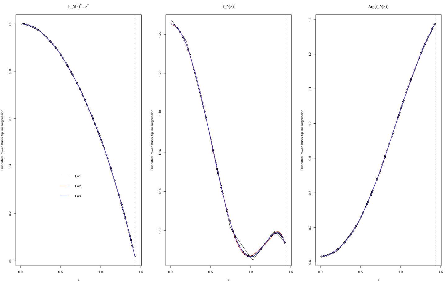
Figure 1: The estimates of critical collapse functions corresponding to $\alpha$-solution of hyperbolic case based on truncated power basis regression of orders $l=\{1,2,3\}$ from a training sample of size $n=100$.

Given a training data of size $n$ from explanatory variable $x$, response variable $y$ and a large set of knots $\{l_{1},\ldots,l_{K}\}$, we first obtain the B-spline basis from (45) and construct the corresponding design matrix ${\bf G}$ from (46). The penalized B-spline estimation can then be re-written as penalized least square method as follows

$${\widehat{\bf\beta}}=\underset{{\bf\beta}}{\arg\min}\left\{||{\bf y}-{\bf G}{\bf\beta}||_{2}^{2}+\lambda^{2}{\bf\beta}^{\top}{\bf D}{\bf\beta}\right\},$$ (48)

where $\lambda$ is the tuning parameter and

$${\bf D}=\left[\begin{array}[]{cc}{\bf 0}_{2\times 2}&{\bf 0}_{2\times K}\\ {\bf 0}_{K\times 2}&{\bf I}_{K\times K}\end{array}\right].$$

From optimization (48), it is easy to show that the penalize B-spline estimates the critical collapse function $g(x)$ at new ${x}_{\text{new}}$ is obtained by

$${\widehat{y}}_{\text{new}}={\widehat{g}}({x}_{\text{new}})={\bf B}({x}_{\text{new}})({\bf G}^{\top}{\bf G}+\lambda{\bf D})^{-1}{\bf G}^{\top}{\bf y}$$ (49)

where ${\bf B}({x}_{\text{new}})=\left(1,B_{1}({x}_{\text{new}}),\ldots,B_{K}({x}_{\text{new}})\right)^{\top}$ and $B_{j}({x}_{\text{new}}),j=1,\ldots,K$ are calculated from (45).

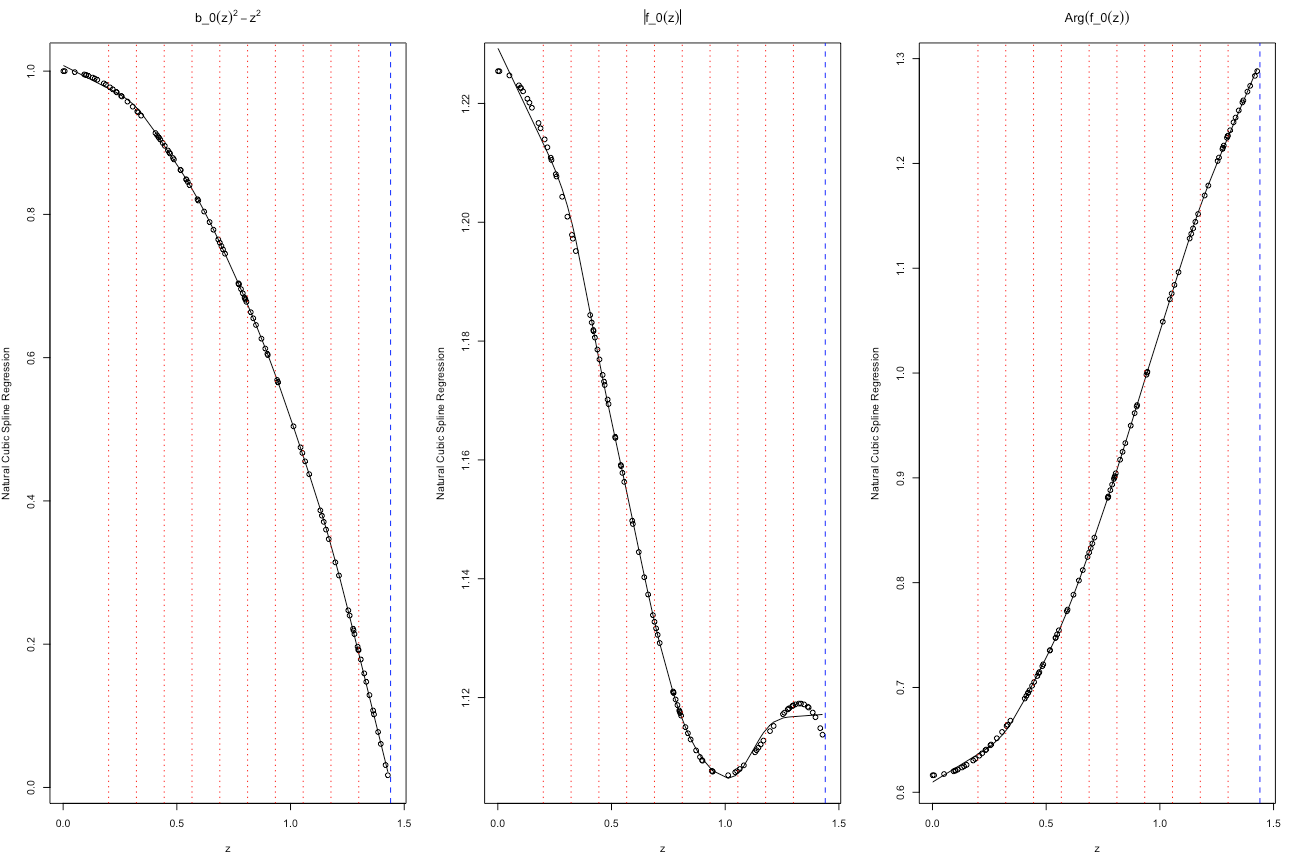
Figure 2: The estimates of critical collapse functions corresponding to $\alpha$-solution of hyperbolic case based on the natural cubic spline regression from a training sample of size $n=100$. The red lines show the locations of the knots.

$K$	Elliptic		Hyperbolic
		$\alpha$-solution	$\beta$-solution	$\gamma$-solution
3	0.0028825	0.0024568	0.0031036	0.0000290
5	0.0013078	0.0000938	0.0004437	0.0000107
8	0.0002640	0.0000104	0.0000209	0.0000110
10	0.0000988	0.0000056	0.0000268	0.0000113
15	0.0001045	0.0000055	0.0000149	0.0000119
20	0.0000552	0.0000050	0.0000057	0.0000129

Table 1: The $\sqrt{\text{MSE}}$ of truncated power basis method of orders $M=3$ with $K=\{3,5,\ldots,20\}$ knots in estimating the critical collapse response function $g(z)=|f_{0}(z)|$ in elliptic and hyperbolic cases based on a training sample of size $n=100$.

As we see from (49), the penalized B-spline estimator requires us to determine the tuning parameter $\lambda$ in estimating the critical collapse function. We apply the idea of cross-validation to find the optimal value of $\lambda$. The idea of cross-validation arises from the fact that the optimal $\lambda$ provides the best fit to the underlying nonlinear function over the entire domain. Let $y_{i}$ and ${\hat{y}}_{i}$ be the observed and predicted responses using $\lambda$ for all training data $i=1,\ldots,n$. To this end, we find the optimal $\lambda$ value, which minimizes the error sum of squares as a measure of goodness of fit. The error sum of squares (RSS) based on each $\lambda$ is given by

$$\text{RSS}(\lambda)=\sum_{i=1}^{n}(y_{i}-{\hat{y}}_{i})^{2}={\bf y}^{\top}{\bf y}-2{\bf y}^{\top}{\bf\widehat{g}}_{\lambda}+{\bf\widehat{g}}_{\lambda}^{\top}{\bf\widehat{g}}_{\lambda},$$

where ${\bf y}=(y_{1},\ldots,y_{n})$ and ${\bf\widehat{g}}_{\lambda}=\left({\bf\widehat{g}}_{\lambda}(x_{1}),\ldots,{\bf\widehat{g}}_{\lambda}(x_{n})\right)$ are vectors of the observed and the predicted responses based on full chain of training data for each $\lambda$.

Generalized cross-validation (GCV) [41] is considered as one of the well-established algorithms to find the optimal $\lambda$ that dramatically reduces the computational burden of the cross-validation. The GCV makes use of the Demmler–Reinsch Orthogonalization approach [42] to find sequentially the predicted responses for each $\lambda$ value. Accordingly, the GCV procedure is carried out as follows: First, we predict the value of nonlinear function ${\bf\widehat{g}}_{\lambda}$ based on all $x$ values in the training data for each $\lambda$ as

$${\bf\widehat{g}}_{\lambda}={\bf G}\left({\bf G}^{\top}{\bf G}+\lambda{\bf D}\right)^{-1}{\bf G}^{\top}{\bf y}.$$

$K$	Elliptic		Hyperbolic
		$\alpha$-solution	$\beta$-solution	$\gamma$-solution
3	0.0120394	0.0080850	0.0073040	0.0015161
5	0.0047826	0.0019024	0.0048836	0.0005355
8	0.0044198	0.0011526	0.0024039	0.0002743
10	0.0036682	0.0009570	0.0016642	0.0002136
15	0.0023819	0.0007245	0.0009556	0.0001528
20	0.0019741	0.0005985	0.0005809	0.0001225

Table 2: The $\sqrt{\text{MSE}}$ of cubic natural spline method with $K=\{3,5,\ldots,20\}$ knots in estimating the critical collapse response function $g(z)=|f_{0}(z)|$ in elliptic and hyperbolic cases based on a training sample of size $n=100$.

In the second step, we apply Cholesky decomposition for symmetric matrix ${\bf G}^{\top}{\bf G}$ and obtain the triangular matrix ${\bf R}$ such that ${\bf G}^{\top}{\bf G}={\bf R}^{\top}{\bf R}$. In step three, we apply singular value decomposition of the symmetric matrix ${\bf R}^{-1}{\bf D}{\bf R}$ and find ${\bf U}\text{diag}({\bf s}){\bf U}^{\top}$. We compute ${\bf A}={\bf G}{\bf R}^{-1}{\bf U}$ and ${\bf b}={\bf A}^{\top}{\bf y}$. Then, ${\bf\widehat{g}}_{\lambda}=\left({\bf\widehat{g}}_{\lambda}(x_{1}),\ldots,{\bf\widehat{g}}_{\lambda}(x_{n})\right)$ is updated by

$${\bf\widehat{g}}_{\lambda}={\bf A}\left(\frac{{\bf b}}{1+\lambda{\bf s}}\right).$$

We perform the above procedure sequentially for all possible $\lambda$ values and obtain the RSS based on all $\lambda$ values; that is RSS($\lambda_{1}$), RSS($\lambda_{2}$) and so on. Finally, the optimal value is the $\lambda$ corresponding to the minimum RSS. This optimal value is henceforth called $\lambda_{\text{GCV}}$. From $\lambda_{\text{GCV}}$ and (49), the penalized B-spline estimator for nonlinear function at the new point ${x}_{\text{new}}$ is derived by

$${\widehat{y}}_{\text{new}}={\widehat{g}}({x}_{\text{new}})={\bf B}({x}_{\text{new}})({\bf G}^{\top}{\bf G}+\lambda_{\text{GCV}}{\bf D})^{-1}{\bf G}^{\top}{\bf y}.$$ (50)

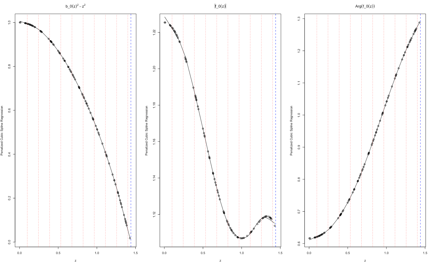
Figure 3: The estimates of critical collapse functions corresponding to $\alpha$-solution of hyperbolic case based on penalized B-spline regression of order $l=1$ from a training sample of size $n=100$. The red lines show the locations of the knots.

5 Numerical Studies

Solutions to axion-dilaton in black holes were recently studied in [26] in both elliptic and hyperbolic spacetime in 4 dimensions. They located only one solution in the elliptic case and three distinctive solutions in the hyperbolic case. Due to the importance of the unperturbed critical collapse functions in the location of the solutions, in [31] we recently utilized polynomial regression, kernel regression and local regression models to estimate the unperturbed critical function. While these polynomial and Fourier-based methods work well in estimating the global behaviour of the nonlinear critical collapse functions, these estimators do not support local properties. This section develops truncated power basis spline, cubic natural spline, and penalized B-spline models in estimating the nonlinear critical collapse functions in elliptic and hyperbolic cases.

In a similar vein to [26], we implemented a numerical optimization to find the critical solutions to the equations of motions in the domain of forward-singularity ($[0,z_{+}]$). This resulted in a unique solution in the interval [0, 2.5] corresponding to the domain of the critical collapse functions in the elliptic space. In the case of hyperbolic space, we found three solutions corresponding to $\alpha$-, $\beta$- and $\gamma$- solutions to the equations of motions. This leads to three domains for the critical collapse functions corresponding to interval [0,1.44] (for $\alpha$-solution), interval [0, 3.30] (for $\beta$-solution) and interval [0, 8.45] (for $\gamma$-solution). Similar to [26, 31], we implemented the optimization search and obtained 2000 observations from each domain of the critical collapse functions $b_{0}^{2}-z^{2},|f_{0}(z)|$ and $\arg f_{0}(z)$ in both elliptic ad hyperbolic spaces. These 2000 observations were then treated as our unknown statistical populations that should be recovered by the statistical models for each interval in elliptic and hyperbolic spaces.

From each observation in the population, we treated the spacetime $z$ coordinate and the value of the nonlinear critical collapse functions as the explanatory variable and response received from the population. We selected a random sample (with replacement) of size $n=100$ from each population of interest for training the statistical models. We then use the training data to estimate the parameters of the truncated power basis spline, cubic natural spline and penalized B-spline models for estimating the three critical collapse functions. To assess the performance of the proposed spline regression models, independently from the training data, we also generated a validation/test sample of size $n=100$ from each population. Suppose $(x_{i,test},y_{i,test}),i=1\ldots,n$ denotes the test sample of size $n$. Using the trained truncated power basis, cubic natural spline and penalized B-spline estimators, we predicted the critical collapse functions at every point $x_{i,test}$ (without using the values of $y_{i,test}$ in the estimation procedure) $i=1\ldots,n$. The predicted response is called ${\widehat{y}}_{i,test},i=1\ldots,n$. We then computed the prediction responses as described above for all critical collapse functions and used the square root of the mean squared error to measure the prediction accuracy of the purposed spline estimation methods. The square root of mean squared error $\sqrt{\text{MSE}}$ is given by

$$\sqrt{\text{MSE}}=\left(1/n\sum_{i=1}^{n}({\widehat{y}}_{i,test}-y_{i,test})^{2}\right)^{1/2}.$$

$\sqrt{\text{MSE}}$ decreases when the proposed spline model predicts more accurately the underlying nonlinear critical collapse function over the entire domain. In other words, the predicted responses (using the spline model) get closer to the responses observed from the nonlinear critical collapse function.

$K$	Elliptic		Hyperbolic
		$\alpha$-solution	$\beta$-solution	$\gamma$-solution
3	0.0111553	0.0073981	0.0071837	0.0018790
5	0.0028832	0.0018389	0.0039828	0.0005865
8	0.0025321	0.0009167	0.0016816	0.0003127
10	0.0019106	0.0007042	0.0011894	0.0002366
15	0.0015122	0.0004346	0.0006268	0.0001317
20	0.0011401	0.0003069	0.0003900	0.0001016

Table 3: The $\sqrt{\text{MSE}}$ of penalized cubic B-spline method with $K=\{3,5,\ldots,20\}$ knots in estimating the critical collapse response function $g(z)=|f_{0}(z)|$ in elliptic and hyperbolic cases based on a training sample of size $n=100$.

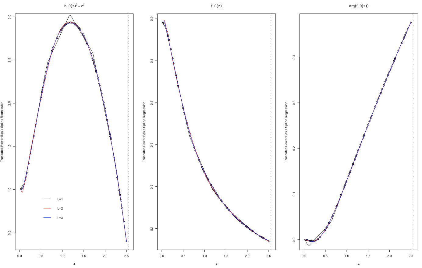
Figure 4: The estimates of critical collapse functions based on truncated power basis regression of orders $m=\{1,2,3\}$ in elliptic case from a training sample of size $n=100$.

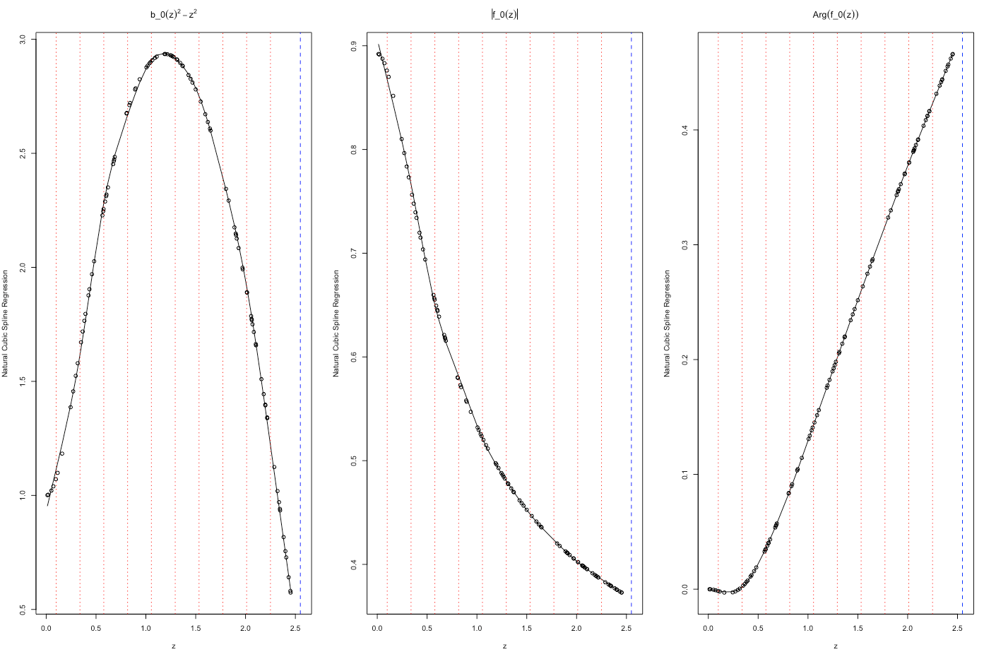
Figure 5: The estimates of critical collapse functions based on the natural cubic spline regression in elliptic case from a training sample of size $n=100$. The red lines show the locations of the knots.

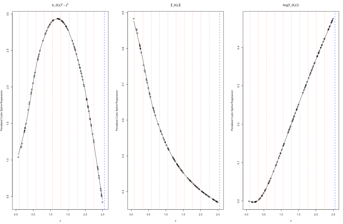
Figure 6: The estimates of critical collapse functions based on penalized B-spline regression of order $l=1$ in elliptic from a training sample of size $n=100$. The red lines show the locations of the knots.

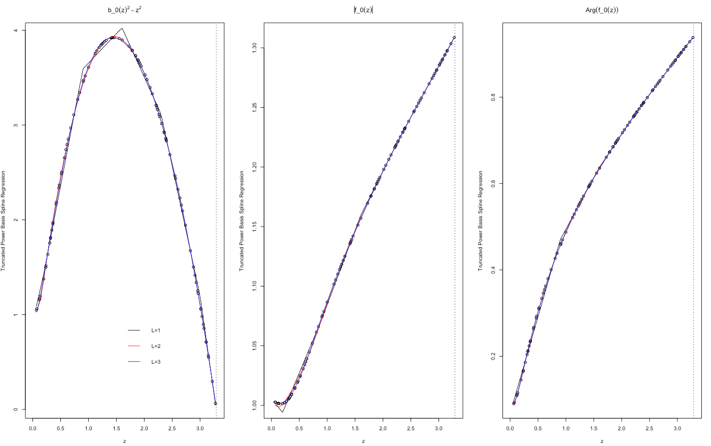
Figure 7: The estimates of critical collapse functions corresponding to $\beta$-solution of hyperbolic case based on truncated power basis regression of orders $l=\{1,2,3\}$ from a training sample of size $n=100$.

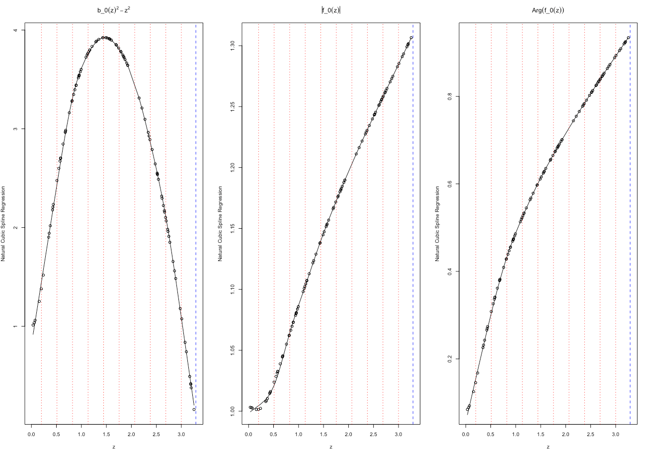
Figure 8: The estimates of critical collapse functions corresponding to $\beta$-solution of hyperbolic case based on natural cubic spline regression from a training sample of size $n=100$. The red lines show the locations of the knots.

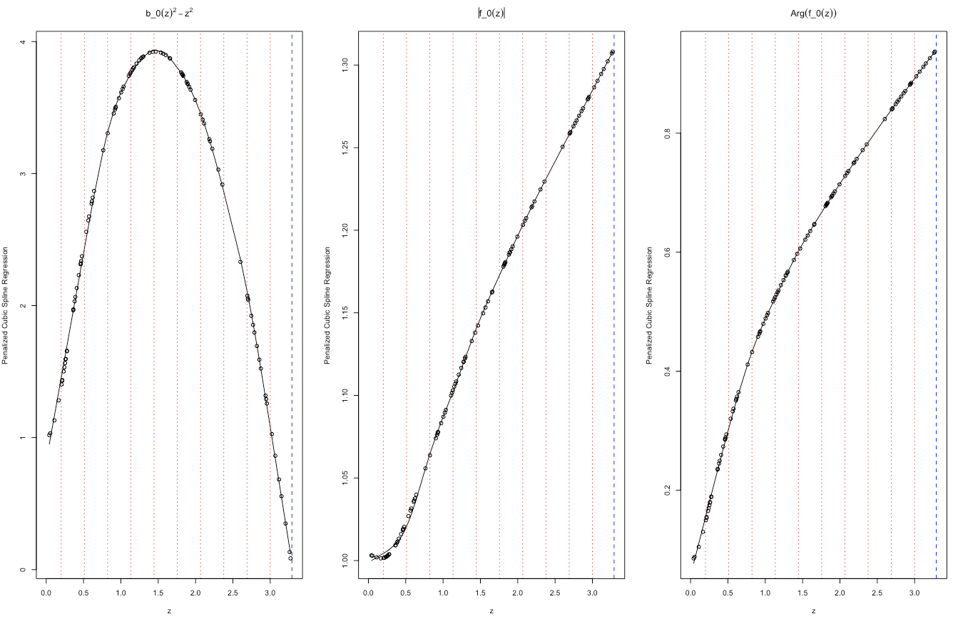
Figure 9: The estimates of critical collapse functions corresponding to $\beta$-solution of hyperbolic case based on penalized B-spline regression of order $l=1$ from a training sample of size $n=100$.The red lines show the locations of the knots.

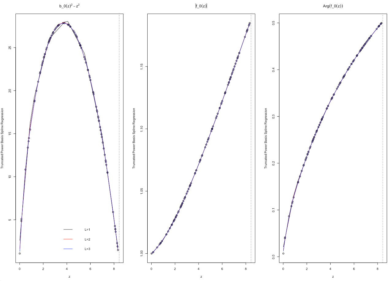
Figure 10: The estimates of critical collapse functions corresponding to $\gamma$-solution of hyperbolic case based on truncated power basis regression of orders $l=\{1,2,3\}$ from a training sample of size $n=100$.

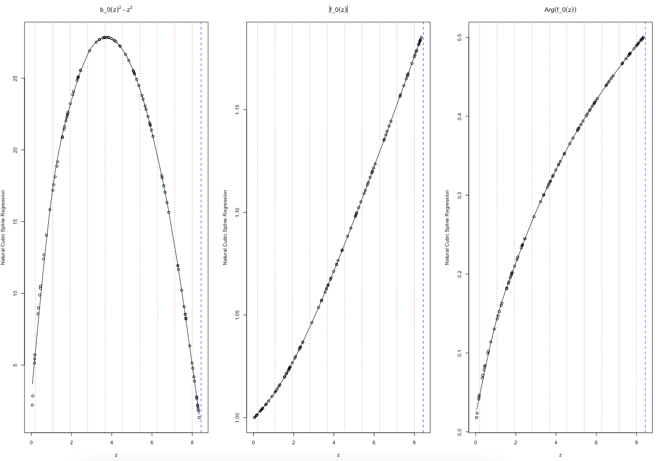
Figure 11: The estimates of critical collapse functions corresponding to $\gamma$-solution of hyperbolic case based on natural cubic spline regression from a training sample of size $n=100$. The red lines show the locations of the knots.

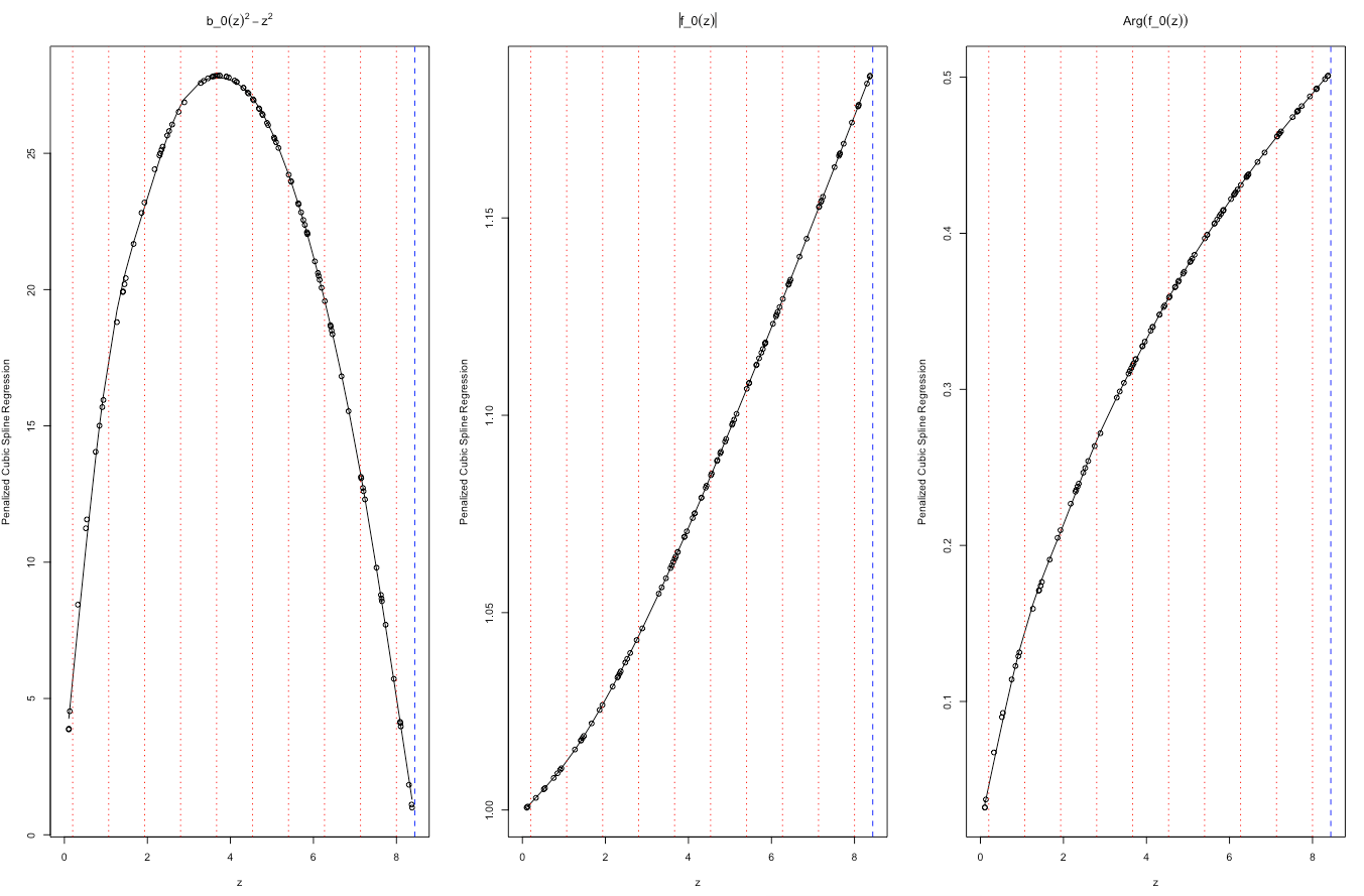
Figure 12: The estimates of critical collapse functions corresponding to $\gamma$-solution of hyperbolic case based on penalized B-spline regression from a training sample of size $n=100$. The red lines show the locations of the knots.

We show the performance of the proposed methods in estimating the critical collapse functions in both elliptic and hyperbolic cases in the following figures and tables. Figures 1, 4, 7 and 10 compare the estimation of critical collapse functions using truncated power basis splines of orders $M=\{1,2,3\}$ in both elliptic ad hyperbolic spaces. Owing to the advantages of the cubic splines, Tables 1-9 show the $\sqrt{\text{MSE}}$ of truncated power basis spline, natural spline and penalized B-spline of order $M=3$. In each table, we illustrate the performance of the estimators using $K=\{3,5,8,10,15,20\}$ knots of equally spaced in the domain of each function. From Tables 1-9, we observe that the prediction error of almost all proposed spline models are less than $10^{-2}$ such that the proposed models can be considered unbiased estimators for the critical collapse functions in both elliptic and hyperbolic spaces (See also Figures 1-12). We observe the $\sqrt{\text{MSE}}$ of the truncated power basis model is smaller than those of natural spline and penalized B-spline models. We also observe that penalized B-spline estimators almost always outperform the natural spline counterparts in predicting the elliptic and hyperbolic cases. Note that introducing more knots does not necessarily improve the performance of the truncated power basis model. There are several reasons for this fact. When $K$ increases, the multicollinearity problem arises in design matrix and consequently the estimation performance of the truncated power basis may not increase or even may decrease (e.g., Table 1 in the case of $\gamma$-solution). Second, the higher polynomial orders may force the truncated power basis to change erratically in the extreme regions while the critical function may not be highly nonlinear in the extreme regions. In this situation, we recommend the natural cubic spline smoother which imposes restrictions on the higher orders in the extreme regions. Given the training data, when $K$ increases, no (or very few) training data may be found in some regions. Thus, the estimation performance of the truncated power basis decreases in these regions. To handle this problem, we recommend the penalized B-spline smoother where sequentially selects the optimal number of knots in estimation procedure. An advantage of the truncated power basis spline is that the method gives us a closed-form, continuous estimator with continuous derivatives of orders $M=\{1,2\}$ in predicting the unperturbed critical collapse functions. This closed form and continuously differentiable estimators can play a high importance in paving the path for researchers to analytically find the critical solutions, critical exponents and mass of black holes.

Given the positive part function from (37), we define $u(z)=(z)^{3}_{+}$. The closed forms of critical collapse functions based on truncated power basis splines of order $M=3$ in elliptic space with knots $\{l_{1},\ldots,l_{5}\}=\{0.1,0.637,1.175,1.712,2.25\}$ are given by

$$\widehat{b_{0}(z)^{2}}= 1-1.37z+31.02z^{2}-91.22z^{3}+88.17u(z-l_{1})$$

$$+3.47u(z-l_{2})-0.35u(z-l_{3})+0.11u(z-l_{4})-0.77u(z-l_{5}),$$ (51)

$$\widehat{|f_{0}(z)|}= 0.89+0.38z-8.15z^{2}+26.62z^{3}-26.32u(z-l_{1})$$

$$-0.45u(z-l_{2})+0.15u(z-l_{3})-0.04u(z-l_{4})+0.22u(z-l_{5}),$$ (52)

$$\widehat{\arg f_{0}(z)}= -0.0005+0.11z-2.13z^{2}+8.32z^{3}-8.48u(z-l_{1})$$

$$+0.08u(z-l_{2})+0.07u(z-l_{3})-0.01u(z-l_{4})+0.07u(z-l_{5}).$$ (53)

The closed forms of critical collapse functions corresponding to $\alpha$-solution in hyperbolic space based on truncated power basis splines of order $M=3$ with knots $\{l_{1},\ldots,l_{5}\}=\{0.2,0.475,0.75,1.025,1.3\}$ are given by

$$\widehat{b_{0}(z)^{2}}= 1-1.76z-4.39z^{2}+2.96z^{3}+6.02u(z-l_{1})$$

$$-6.53u(z-l_{2})-2.20u(z-l_{3})-1.10u(z-l_{4})+9.01u(z-l_{5}),$$ (54)

$$\widehat{|f_{0}(z)|}= 1.22-0.0006z-0.27z^{2}+0.04z^{3}+0.18u(z-l_{1})$$

$$+0.13u(z-l_{2})-0.33u(z-l_{3})-0.69u(z-l_{4})-0.95u(z-l_{5}),$$ (55)

$$\widehat{\arg f_{0}(z)}= 0.61-0.001z+0.44z^{2}-0.003z^{3}+0.04u(z-l_{1})$$

$$-0.23u(z-l_{2})-0.39u(z-l_{3})+0.22u(z-l_{4})+1.64u(z-l_{5}).$$ (56)

The closed forms of critical collapse functions corresponding to $\beta$-solution in hyperbolic space based on truncated power basis splines of order $M=3$ with knots $\{l_{1},\ldots,l_{5}\}=\{0.2,0.9,1.6,2.3,3\}$ are given by

$$\widehat{b_{0}(z)^{2}}= 1.05-2.20z+30.80z^{2}-50.54z^{3}+49.82u(z-l_{1})$$

$$+1.12u(z-l_{2})-0.38u(z-l_{3})+0.11u(z-l_{4})-0.90u(z-l_{5}),$$ (57)

$$\widehat{|f_{0}(z)|}= 1-0.04z+0.15z^{2}+0.05z^{3}-0.15u(z-l_{1})$$

$$+0.1u(z-l_{2})-0.004u(z-l_{3})+0.005u(z-l_{4})-0.02u(z-l_{5}),$$ (58)

$$\widehat{\arg f_{0}(z)}= 0.08-0.28z+4.46z^{2}-7.78z^{3}+7.81u(z-l_{1})$$

$$+0.02u(z-l_{2})-0.05u(z-l_{3})+0.01u(z-l_{4})-0.11u(z-l_{5}).$$ (59)

The closed forms of critical collapse functions corresponding to $\gamma$-solution in hyperbolic space based on truncated power basis splines of order $M=3$ with knots $\{l_{1},\ldots,l_{5}\}=\{1,2.5,4,5.5,7\}$ are given by

$$\widehat{b_{0}(z)^{2}}= 1.01+26.62z-14.61z^{2}+4.52z^{3}-4.41u(z-l_{1})$$

$$-0.048u(z-l_{2})-0.047u(z-l_{3})+0.0049u(z-l_{4})-0.02u(z-l_{5}),$$ (60)

$$\widehat{|f_{0}(z)|}= 0.99-.04z+.01z^{2}+.0007z^{3}+.0006u(z-l_{1})$$

$$-.0009u(z-l_{2})+.0001u(z-l_{3})+.00003u(z-l_{4})-.00001u(z-l_{5}).$$ (61)

$$\widehat{\arg f_{0}(z)}= .009+.203z-.108z^{2}-.0334z^{3}-.0327u(z-l_{1})$$

$$-.00005u(z-l_{2})-.00044u(z-l_{3})+.00006u(z-l_{4})-.000198u(z-l_{5}).$$ (62)

6 Summary and Concluding Remarks

In this paper, we investigated the properties of the spline regression models in estimating the nonlinear critical collapse functions for axion-dilaton system in elliptic and hyperbolic cases in four dimensions. The spline regression models include truncated power basis, natural cubic spline and penalized B-splines. The truncated power basis and natural spline use knots over the domain of a nonlinear function to accommodate the local changes in the prediction using the basis functions and hence we do not require to adjust the global pattern of the models. In addition to using knots, the penalized B-spline regression model uses the constrained optimization to reach the optimal level of smoothness and avoid overfitting problem. Through various numerical studies, we evaluated the performance of the proposed spline models in estimating the critical collapse functions. We observed that the error of the developed estimators, on average, are almost less than $10^{-2}$ such that all the estimators can be considered as an unbiased estimators for the critical collapse functions. In addition to the accuracy of the proposed models, the truncated power basis spline provides us a closed-form, continuous estimator with continuous derivatives of orders $M=\{1,2\}$ in predicting the unperturbed critical collapse functions. This analytical estimators can be of high importance to pave the path for finding analytically the solutions, critical exponents and mass of black holes.

Appendix

$K$	Elliptic		Hyperbolic
		$\alpha$-solution	$\beta$-solution	$\gamma$-solution
3	0.0222907	0.0004868	0.0332154	0.0679797
5	0.0049895	0.0000634	0.0135313	0.0680210
8	0.0005913	0.0000074	0.0031689	0.0664356
10	0.0001874	0.0000034	0.0016043	0.0649515
15	0.0004048	0.0000037	0.0004153	0.0614526
20	0.0001411	0.0000048	0.0001062	0.0596425

Table 4: The $\sqrt{\text{MSE}}$ of truncated power basis method of orders $M=3$ with $K=\{3,5,\ldots,20\}$ knots in estimating the critical collapse response function $g(z)=b_{0}^{2}(z)-z^{2}$ in elliptic and hyperbolic cases based on a training sample of size $n=100$.

$K$	Elliptic		Hyperbolic
		$\alpha$-solution	$\beta$-solution	$\gamma$-solution
3	0.0007897	0.0009433	0.0015890	0.0006771
5	0.0003643	0.0001183	0.0015586	0.0006875
8	0.0001263	0.0000113	0.0005004	0.0006727
10	0.0000584	0.0000089	0.0002765	0.0006613
15	0.0000931	0.0000089	0.0000794	0.0006356
20	0.0000290	0.0000099	0.0000194	0.0006224

Table 5: The $\sqrt{\text{MSE}}$ of truncated power basis method of orders $M=3$ with $K=\{3,5,\ldots,20\}$ knots in estimating the critical collapse response function $g(z)=\arg f_{0}(z)$ in elliptic and hyperbolic cases based on a training sample of size $n=100$.

$K$	Elliptic		Hyperbolic
		$\alpha$-solution	$\beta$-solution	$\gamma$-solution
3	0.0583561	0.0100865	0.1012991	1.4876654
5	0.0452239	0.0045656	0.0472993	0.8784532
8	0.0274994	0.0025943	0.0439414	0.6357770
10	0.0209406	0.0020206	0.0396018	0.5490553
15	0.0128638	0.0014594	0.0323031	0.4459167
20	0.0103324	0.0012106	0.0274119	0.3893207

Table 6: The $\sqrt{\text{MSE}}$ of cubic natural spline method with $K=\{3,5,\ldots,20\}$ knots in estimating the critical collapse response function $g(z)=b_{0}^{2}(z)-z^{2}$ in elliptic and hyperbolic cases based on a training sample of size $n=100$.

$K$	Elliptic		Hyperbolic
		$\alpha$-solution	$\beta$-solution	$\gamma$-solution
3	0.0145808	0.0182347	0.0175141	0.0077258
5	0.0035752	0.0040297	0.0046769	0.0045959
8	0.0007587	0.0018753	0.0047694	0.0033778
10	0.0002901	0.0014674	0.0047028	0.0029812
15	0.0001175	0.0010645	0.0041953	0.0025177
20	0.0001081	0.0008880	0.0037143	0.0022268

Table 7: The $\sqrt{\text{MSE}}$ of cubic natural spline method with $K=\{3,5,\ldots,20\}$ knots in estimating the critical collapse response function $g(z)=\arg f_{0}(z)$ in elliptic and hyperbolic cases based on a training sample of size $n=100$.

$K$	Elliptic		Hyperbolic
		$\alpha$-solution	$\beta$-solution	$\gamma$-solution
3	0.0594606	0.0088410	0.1029377	1.6690824
5	0.0378520	0.0029216	0.0339346	0.9070288
8	0.0188786	0.0013406	0.0275224	0.6636289
10	0.0132785	0.0009962	0.0256748	0.5671875
15	0.0093517	0.0005840	0.0197771	0.4318121
20	0.0069107	0.0004166	0.0166023	0.3937617

Table 8: The $\sqrt{\text{MSE}}$ of penalized cubic B-spline method with $K=\{3,5,\ldots,20\}$ knots in estimating the critical collapse response function $g(z)=b_{0}^{2}(z)-z^{2}$ in elliptic and hyperbolic cases based on a training sample of size $n=100$.

$K$	Elliptic		Hyperbolic
		$\alpha$-solution	$\beta$-solution	$\gamma$-solution
3	0.0123415	0.0188509	0.0178855	0.0095065
5	0.0030677	0.0025941	0.0035336	0.0051307
8	0.0006357	0.0009867	0.0028396	0.0038707
10	0.0002447	0.0007396	0.0029189	0.0033959
15	0.0000877	0.0004281	0.0025423	0.0027116
20	0.0000719	0.0003076	0.0022254	0.0025339

Table 9: The $\sqrt{\text{MSE}}$ of penalized cubic B-spline method with $K=\{3,5,\ldots,20\}$ knots in estimating the critical collapse response function $g(z)=\arg f_{0}(z)$ in elliptic and hyperbolic cases based on a training sample of size $n=100$.

References

- [1] M.W. Choptuik, Universality and Scaling in Gravitational Collapse of a Massless Scalar Field, Phys. Rev. Lett. 70, 9 (1993).
- [2] D. Christodoulou, “The Problem of a Self-gravitating Scalar Field,” Commun. Math. Phys. 105 (1986) 337; “Global Existence of Generalized Solutions of the Spherically Symmetric Einstein Scalar Equations in the Large,” Commun. Math. Phys. 106 (1986) 587;“The Structure and Uniqueness of Generalized Solutions of the Spherically Symmetric Einstein Scalar Equations,” Commun. Math. Phys. 109 (1987) 591.
- [3] R. S. Hamade and J. M. Stewart, “The Spherically symmetric collapse of a massless scalar field,” Class. Quant. Grav. 13 (1996) 497 [arXiv:gr-qc/9506044].
- [4] C. Gundlach, “Critical phenomena in gravitational collapse,” Phys. Rept. 376 (2003) 339 [gr-qc/0210101].
- [5] T. Koike, T. Hara, and S. Adachi, “Critical Behavior in Gravitational Collapse of Radiation Fluid: A Renormalization Group (Linear Perturbation) Analysis,” Phys. Rev. Lett. 74 (1995) 5170 [gr-qc/9503007].
- [6] L. Alvarez-Gaume, C. Gomez and M. A. Vazquez-Mozo, “Scaling Phenomena in Gravity from QCD,” Phys. Lett. B 649 (2007) 478 [hep-th/0611312].
- [7] M. Birukou, V. Husain, G. Kunstatter, E. Vaz and M. Olivier, “Scalar field collapse in any dimension,” Phys. Rev. D 65 (2002) 104036 [gr-qc/0201026].
- [8] V. Husain, G. Kunstatter, B. Preston and M. Birukou, “Anti-de Sitter gravitational collapse,” Class. Quant. Grav. 20 (2003) L23 [gr-qc/0210011].
- [9] E. Sorkin and Y. Oren, “On Choptuik’s scaling in higher dimensions,” Phys. Rev. D 71, 124005 (2005) [arXiv:hep-th/0502034].
- [10] J. Bland, B. Preston, M. Becker, G. Kunstatter and V. Husain, “Dimension-dependence of the critical exponent in spherically symmetric gravitational collapse,” Class. Quant. Grav. 22 (2005) 5355 [gr-qc/0507088].
- [11] E. W. Hirschmann and D. M. Eardley, “Universal scaling and echoing in gravitational collapse of a complex scalar field,” Phys. Rev. D 51 (1995) 4198 [gr-qc/9412066].
- [12] J. V. Rocha and M. Tomašević, “Self-similarity in Einstein-Maxwell-dilaton theories and critical collapse,” Phys. Rev. D 98 (2018) no.10, 104063 [arXiv:1810.04907 [gr-qc]].
- [13] L. Alvarez-Gaume, C. Gomez, A. Sabio Vera, A. Tavanfar and M. A. Vazquez-Mozo,“Critical gravitational collapse: towards a holographic understanding of the Regge region,” Nucl. Phys. B 806 (2009) 327 [arXiv:0804.1464 [hep-th]].
- [14] C. R. Evans and J. S. Coleman, “Observation of critical phenomena and selfsimilarity in the gravitational collapse of radiation fluid,” Phys. Rev. Lett. 72 (1994) 1782 [gr-qc/9402041].
- [15] D. Maison, “Non-Universality of Critical Behaviour in Spherically Symmetric Gravitational Collapse,” Phys. Lett. B 366 (1996) 82 [gr-qc/9504008].
- [16] A. Strominger and L. Thorlacius, “Universality and scaling at the onset of quantum black hole formation,” Phys. Rev. Lett. 72 (1994) 1584 [hep-th/9312017].
- [17] E. W. Hirschmann and D. M. Eardley, ‘Critical exponents and stability at the black hole threshold for a complex scalar field,” Phys. Rev. D 52 (1995) 5850 [gr-qc/9506078].
- [18] A. M. Abrahams and C. R. Evans, “Critical behavior and scaling in vacuum axisymmetric gravitational collapse,” Phys. Rev. Lett. 70 (1993) 2980.
- [19] L. Alvarez-Gaume, C. Gomez, A. Sabio Vera, A. Tavanfar and M. A. Vazquez-Mozo, “Critical formation of trapped surfaces in the collision of gravitational shock waves,” JHEP 0902, 009 (2009) [arXiv:0811.3969 [hep-th]].
- [20] E. W. Hirschmann and D. M. Eardley, “Criticality and bifurcation in the gravitational collapse of a selfcoupled scalar field,” Phys. Rev. D 56 (1997) 4696 [gr-qc/9511052].
- [21] J. M. Maldacena, “The Large N limit of superconformal field theories and supergravity,”Int. J. Theor. Phys. 38 (1999), 1113-1133, Adv. Theor. Math. Phys. 2, arXiv:hep-th/9711200, E. Witten, “Anti-de Sitter space and holography,” Adv. Theor. Math. Phys. 2 (1998), 253-291,hep-th/9802150, S. Gubser, I. R. Klebanov and A. M. Polyakov, “Gauge theory correlators from noncritical string theory,” Phys. Lett. B 428 (1998), 105-114, hep-th/9802109.
- [22] D. Birmingham, “Choptuik scaling and quasinormal modes in the AdS / CFT correspondence,” Phys. Rev. D 64 (2001), 064024 [arXiv:hep-th/0101194 [hep-th]].
- [23] E. Hatefi, A. Nurmagambetov and I. Park, “ADM reduction of IIB on to dS braneworld,” JHEP 04 (2013), 170, arXiv:1210.3825 , “ entropy of branes from dielectric effect,” Nucl. Phys. B 866 (2013), 58-71, arXiv:1204.2711, S. de Alwis, R. Gupta, E. Hatefi and F. Quevedo, “Stability, Tunneling and Flux Changing de Sitter Transitions in the Large Volume String Scenario,” JHEP 11 (2013), 179, arXiv:1308.1222.
- [24] A. Ghodsi and E. Hatefi, “Extremal rotating solutions in Horava Gravity,” Phys. Rev. D 81 (2010) 044016 [arXiv:0906.1237 [hep-th]].
- [25] R. S. Hamade, J. H. Horne and J. M. Stewart, “Continuous Self-Similarity and -Duality,” Class. Quant. Grav. 13 (1996) 2241 [arXiv:gr-qc/9511024].
- [26] R. Antonelli and E. Hatefi, “On self-similar axion-dilaton configurations,” , JHEP 03 (2020), 074 [arXiv:1912.00078 [hep-th]].
- [27] L. Álvarez-Gaumé and E. Hatefi, “Critical Collapse in the Axion-Dilaton System in Diverse Dimensions,” Class. Quant. Grav. 29 (2012) 025006 [arXiv:1108.0078 [gr-qc]].
- [28] L. Álvarez-Gaumé and E. Hatefi, “More On Critical Collapse of Axion-Dilaton System in Dimension Four,” JCAP 1310 (2013) 037 [arXiv:1307.1378 [gr-qc]].
- [29] R. Antonelli and E. Hatefi, “On Critical Exponents for Self-Similar Collapse,” JHEP 03 (2020), 180 [arXiv:1912.06103 [hep-th]].
- [30] E. Hatefi and A. Kuntz, “On Perturbation Theory and Critical Exponents for Self-Similar Systems,” Eur. Phys. J. C 81 (2021) no.1, 15 [arXiv:2010.11603 [hep-th]].
- [31] E. Hatefi and A. Hatefi, “Estimation of Critical Collapse Solutions to Black Holes with Nonlinear Statistical Models,” [arXiv:2110.07153 [gr-qc]].
- [32] A. Sen, “Strong - weak coupling duality in four-dimensional string theory,” Int. J. Mod. Phys. A 9 (1994) 3707 [hep-th/9402002].
- [33] J. H. Schwarz, “Evidence for nonperturbative string symmetries,” Lett. Math. Phys. 34 (1995) 309 [hep-th/9411178].
- [34] M.B. Green, J.H. Schwarz and E. Witten, 1987 Superstring Theory Vols I,II, Cambridge University Press,
- [35] J. Polchinski, 1998 String Theory, Vols I,II, Cambridge University Press
- [36] A. Font, L. E. Ibanez, D. Lust and F. Quevedo, “Strong - weak coupling duality and nonperturbative effects in string theory,” Phys. Lett. B 249 (1990) 35.
- [37] D. M. Eardley, E. W. Hirschmann and J. H. Horne, “S duality at the black hole threshold in gravitational collapse,” Phys. Rev. D 52 (1995) 5397 [arXiv:gr-qc/9505041].
- [38] E. Hatefi and E. Vanzan, “On Higher Dimensional Self-Similar Axion-Dilaton Solutions,” Eur. Phys. J. C 80 (2020), 10 [arXiv:2005.11646 [hep-th]].
- [39] C. De Boor, “A practical guide to splines,” New York: Springer-Verlag, (2001).
- [40] F. E. Harrell Jr, “Regression modeling strategies: with applications to linear models, logistic and ordinal regression, and survival analysis,” springer, (2015).
- [41] PHC. Eilers and BD. Marx, “Flexible smoothing with B-splines and penalties”, Statistical Science, 11 (1996), 89–121.
- [42] D. Ruppert, M.P. Wand, and R.J. Carroll, “Semiparametric Regression”, Cambridge University Press, New York (2003).