Exact Trajectory Control for the non-Markovian Quantum Systems

Abstract

We propose a systematic scheme to engineer quantum states of a quantum system governed by a time-convolutionless non-Markovian master equation. According to the idea of the reverse engineering, the general algebraic equation to determine the control parameters, such as coherent and incoherent control fields, are presented. Without artificially engineering the time-dependent decay rates and persisting the environment-induced Lamb shifts, the quantum state can still be transferred into the target state with a finite period of time along an arbitrary designed trajectory in Hilbert space strictly. As an application, we apply our scheme to a driven two-level non-Markovian system, and realize the instantaneous steady state tracking and the complete population inversion with control parameters which are available in experimental-settings.

I Introduction

Driving quantum systems, especially open quantum systems, to desired target states with very high fidelity is a central goal in quantum sciences and technologies, to realize efficient and scalable devices beyond the current state of proof-of-principle demonstrations Koch2019 ; Osnaghi2001 ; Hacohen2018 . For controlling open quantum systems with Markovian dynamics, many enlightening schemes have been proposed to control open quantum systems, such as the adiabatic steady state scheme Venuti2017 , the shortcut to equilibration scheme Dann2019 , the dissipative steady state preparing scheme Zippilli2021 ; Zheng2021 , and the mixed-state inverse engineering scheme Wu2021 . These schemes transfer the quantum state into the target steady state with a satisfactory fidelity.

But to engineer a quantum state of the non-Markovian quantum system is a different matter. Due to the memory effects of the environment, the next state of a non-Markovian quantum system is determined by each of its previous states Liu2019 . The decay rates are time-dependent, and may temporarily acquire negative values Zhang2012 . This negative decay rate pushes the information (coherence or/and energy) to flow back into the open quantum system after the information dissipates into the environment Li2018 . Therefore, to drive the non-Markovian quantum systems into a desired target state along an exact and designable trajectory definitely is a non-trivial task.

In this paper, we focus on this issue, and propose a control scheme for the non-Markovian quantum systems, which are governed by the time-convolutionless master equation Gasbarri2018 . By parameterizing the trajectory of the quantum state from the initial state to the target state, the control parameters can be determined by reversely engineering time-dependent control Liouvillians. In this way, the quantum state of the non-Markovian quantum system is transfered into the target state along the parameterized trajectory strictly. It should be emphasized that, since the spectrum density of the environment is difficult to be engineered in the experiments Jorgensen2020 , we do not select the decay rates as a means of incoherent control. Although the time-dependent decay rates draw the quantum state out of the trajectory, our scheme can eliminate this effect and keep the quantum state on the designed trajectory. We exam our scheme by applying it on the quantum state engineering tasks of a driven two-level non-Markovian system. The instantaneous steady state tracking and the complete population inversion are realized. In this scenario, the two-level non-Markovian systems are not only kinematically controllable, but also dynamically controllable, which is impracticable for the Markovian case.

This paper is organized as follows. In Sec.II, we present the exact trajectory control scheme for the non-Markovian quantum systems governed by the time-convolutionless master equation. Taking a non-Markovian two-level system as an example, the instantaneous steady state tracking and the population inversion are considered in Sec.III. And we show that, attributing to the information backflows, the population can be completely transferred into the excited state of the two-level system with available control parameters in experiments. Finally, we give conclusions and discussions in Sec.IV.

II The Method

In this work, we consider open quantum systems, where the coupling to a reservoir leads to a non-Markovian dynamics for the system density matrix $\rho(t)$, described by a time-convolutionless master equation in the Lindblad form

$$\partial_{t}\rho(t) = \hat{\mathcal{L}}[\rho]$$ (1)

$$= -i[{H}(t),{\rho}]+\sum_{\alpha}\gamma_{\alpha}(t)\mathcal{D}[L_{\alpha}](\rho),$$

where $H(t)$ is the Hamiltonian containing the coherent controls on the system and the Lamb shifts induced by the coupling to the reservoir, while $\mathcal{D}[L_{\alpha}]$ is the Lindbladian with a Lindblad operator $L_{\alpha}$,

$$\mathcal{D}[L_{\alpha}](\rho) = 2\,L_{\alpha}(t){\rho}L_{\alpha}^{\dagger}(t)-\{L_{\alpha}^{\dagger}(t)L_{\alpha}(t),{\rho}\}.$$ (2)

Each Lindblad operator $L_{\alpha}(t)$ is associated with a dissipation channel occurring at the time-dependent rate $\gamma_{\alpha}(t)$. We consider the case where $H(t)$, $\gamma_{\alpha}(t)$ and $L_{\alpha}(t)$ are time-dependent. This kind of master equation can be applied for examples to photonic quantum systems Vega2017 and mesoscopic electron-phonon systems Pereverzev2006 .

Since the time-convolutionless master equation is linear in $\rho(t)$, it is convenient to describe this master equation as a superoperator formalism in Hilbert-Schmidt space Minganti2018 , wherein the density matrix is represented by a $N^{2}$-dimensional vector

$$|{\rho(t)}\rangle\rangle=(\rho_{0}(t),\rho_{1}(t),...,\rho_{N^{2}-1}(t))^{\dagger},$$ (3)

where $\rho_{i}(t)$ is the $i$-th component of $|{\rho(t)}\rangle\rangle$ with a time-independent basis $B_{i}$ of the Hilbert-Schmidt space satisfying $\rho_{i}(t)=\text{Tr}[\rho(t)B_{i}]$. On the other hand, the Liouvillian superoperator becomes a $N^{2}\times N^{2}$ time-dependent supermatrix $\mathcal{L}(t)$ whose elements are given by $\mathcal{L}_{ij}(t)=\text{Tr}[B_{i}^{\dagger}(\hat{\mathcal{L}}[B_{j}])]$. Then the master equation as shown in Eq.(1) now reads

$$\partial_{t}|{\rho(t)}\rangle\rangle=\mathcal{L}(t)|{\rho(t)}\rangle\rangle,$$ (4)

with the Liouvillian supermatrix

$$\mathcal{L}(t) = -i[H\otimes I-I\otimes H^{\text{T}}]$$ (5)

$$+ \sum_{\alpha}\gamma_{\alpha}\left(2L_{\alpha}\otimes L_{\alpha}^{*}-L_{\alpha}^{\dagger}L_{\alpha}\otimes I-I\otimes L_{\alpha}^{\text{T}}L_{\alpha}^{*}\right),$$

where $A^{\text{T}}$ denotes the transposition of the operator $A$ and $I$, is the identity operator.

The aim of the control scheme is to transfer the quantum system from a known and arbitrary initial state $\rho(0)$ to a desired target state $\rho(t_{f})$ along a preset trajectory. The choice on the bases of the Hilbert-Schmidt is not unique, and the principle on this choice is determined by how to simplify complexity for obtaining the feasible control parameters in the Liouvillian superoperator. Without the loss of generality, the basis set of the Hilbert-Schmidt space can be chosen as the SU($N$) Hermitian generators $\{T_{i}\}_{i=1}^{N^{2}-1}$ and the identify operator $T_{0}\equiv I$. Thus the density matrix can be expanded by these bases, and yields

$$|\varrho(t)\rangle\rangle=\frac{1}{N}\left(|I\rangle\rangle+\sqrt{\frac{N(N-1)}{2}}\sum_{i=1}^{N^{2}-1}r_{i}|T_{i}\rangle\rangle\right),$$ (6)

where $\vec{r}=(r_{1},r_{2},...,r_{N^{2}-1})$ is the generalized Bloch vector with $\sum_{i}|r_{i}|^{2}<1$. Within this notation, the density matrix can be parameterized by $N^{2}-1$ independent coefficients.

On the other hand, the Liouvillian superoperator contains all of the control parameters which can be applied in the real-world experimental setting. The control on the quantum system comes from two manners, i.e., the coherent control and the incoherent control. The coherent controls on the quantum system applied in the experiment are contained in the Hamiltonian of the Liouvillian superoperator. By using the SU($N$) Hermitian generators $\{T_{i}\}_{i=0}^{N^{2}-1}$ ( $T_{0}\equiv I$ is the identify operator), the Hamiltonian can be expressed as

$$H(t)=\sum_{i=0}^{N^{2}-1}c_{i}(t)\,T_{i},$$ (7)

where $c_{i}(t)$ denotes the control parameter for the coherent operation $T_{i}$ on the system. The incoherent controls come from the couplings to the environment, which are reflected in the master equation by the Linbladian. Generally, the Lindblad operators can be written as superpositions of the SU($N$) Hermitian generators, such as

$$L_{\alpha}(t)=\sum_{j=1}^{N^{2}-1}l_{j}^{(\alpha)}(t)\,T_{j}$$ (8)

with complex expansion coefficients $l_{j}^{(\alpha)}(t)$. Here we assume that these complex coefficients $\{l^{(\alpha)}_{j}(t)\}$ include incoherent control parameters which are tunable in experiment and influence the system via incoherent manners.These incoherent control parameters include, but not limited to, the main excitation numbers of the environment Basilewitsch2019 ; Shabani2016 , the correlation of the environment Seetharam2021 , even extra noises Pechen2016 . As the restriction on our scheme, the correlation functions of the environment are invariant. Thus the decay rates and the Lamb shifts caused by the interaction between the open quantum systems and the environments can not be changed artificially, which distinguishes our scheme from pervious schemes on this topic Alipour2020 .

Here we are in the position to determine all of the control parameters (coherent and incoherent) reversely. In fact, the density operator vector is the solution of Eq.(4). Our scheme is to preset the density operator $\rho(t)$, and then to determine the control parameters $\{c_{i}(t),l^{(\alpha)}_{j}(t)\}$ by Eq.(4). At the beginning, we parameterize the density operator by the generalized Bloch vector as shown in Eq.(6). The initial and final Bloch vectors have to correspond to the initial and target state of the control task. Thus the time-dependent Bloch vector corresponds to a trajectory of the quantum state in the Hilbert space, which connects the initial state and target state. Then we deal with the Liouvillian supermatix. The elements of the Liouvillian supermatrix can be determined by $\mathcal{L}_{ij}(t)=\text{Tr}[T_{i}^{\dagger}(\hat{\mathcal{L}}[T_{j}])]$. In order to distinguish the coherent and incoherent control manners, we divide the Liouvillian supermatrix into three parts. Thus, we rewrite the time-convolutionless master equation in components of the generalized Bloch vector,

$$\partial_{t}r_{i}(t)=\sum_{j=1}^{N^{2}-1}\left(\mathcal{C}_{ij}+\mathcal{I}_{ij}\right)\,r_{j}(t)+\mathcal{L}^{0}_{i}.$$ (9)

The coherent part reads

$$\mathcal{C}_{ij}=\sum_{k=1}^{N^{2}-1}c_{k}(t)\,\frac{f_{kji}}{2}$$ (10)

and the incoherent part takes the form

$$\mathcal{I}_{ij}=\sum_{m,n=0}^{N^{2}-1}\left(\sum_{\alpha}\gamma_{\alpha}l_{m}^{(\alpha)}(t)l_{n}^{(\alpha)*}(t)\right)s_{mn,ji}$$ (11)

with

$$s_{mn,ji} = \frac{1}{2N}\left(\delta_{im}\,\delta_{jn}-\delta_{mn}\,\delta_{ij}\right)$$ (12)

$$+\frac{1}{4}\sum_{k=1}^{N^{2}-1}\left(\left(i\,f_{jnk}+d_{jnk}\right)\left(i\,f_{imk}+d_{imk}\right)\right.$$

$$\left.-\left(i\,f_{mnk}+d_{mnk}\right)\,d_{kji}\right),$$

where $f_{ijk}$ and $d_{ijk}$ are the structure constants and the d-coefficients of the SU($N$) Lie algebra, respectively. Moreover, the last terms in Eq.(9) can be written as

$$\mathcal{L}_{k}^{0} = \sum_{\alpha}\gamma_{\alpha}(t)\left(\sum_{i,j=1}^{N^{2}-1}l_{i}^{(\alpha)}(t)l_{j}^{(\alpha)*}(t)g_{ijk}\right),$$

with $g_{ijk}=\left(\left(i\,f_{jik}+d_{jik}\right)-\left(i\,f_{ijk}+d_{ijk}\right)\right)$. The derivation of the coherent and incoherent parts of the Liouvillian supermatrix can be found in Appendix A.

In fact, Eq.(9) is not only linear to the components of the Bloch vector, but also linear to the control parameters $\{c_{i}(t),\sum_{\alpha}\gamma_{\alpha}l^{(\alpha)}_{i}(t)l^{(\alpha)*}_{j}(t)\}$. Here, we further assume that there is only one tunable incoherent control parameter in every Lindbladian $\mathcal{D}[L_{\alpha}]$, i.e., $l^{(\alpha)}_{i}(t)=\sqrt{\tilde{c}_{\alpha}(t)}\tilde{l}^{(\alpha)}_{i}$, where $\tilde{c}_{\alpha}(t)$ is a real incoherent control parameter and $\{\tilde{l}^{(\alpha)}_{i}\}$ are time-independent expansion coefficients. Thus, we have $\sum_{\alpha}\gamma_{\alpha}l^{(\alpha)}_{i}(t)l^{(\alpha)*}_{j}(t)=\sum_{\alpha}\gamma_{\alpha}\tilde{c}_{\alpha}(t)\tilde{l}^{(\alpha)}_{i}\tilde{l}^{(\alpha)*}_{j}$. In this notation, the equations of the control parameters are given by

$$\sum_{j}\Lambda^{c}_{ij}c_{j}+\sum_{\alpha}\gamma_{\alpha}\left(\Lambda^{i}_{\alpha\,i}+\Lambda^{0}_{\alpha\,i}\right)\tilde{c}_{\alpha}-\partial_{t}r_{i}(t)=0,\,\forall i$$

(13)

where the coefficient matrixes for the coherent control and incoherent parameters are

$$\Lambda^{c}_{ij} = \sum_{k=1}^{N^{2}-1}r_{k}(t)\,\frac{f_{jki}}{2},$$

$$\Lambda^{i}_{\alpha\,i} = \sum_{j,m,n=0}^{N^{2}-1}r_{j}(t)\left(\tilde{l}_{m}^{(\alpha)}(t)\tilde{l}_{n}^{(\alpha)*}(t)\right)s_{mn,ji},$$

$$\Lambda^{0}_{\alpha\,i} = \sum_{j,k=1}^{N^{2}-1}\tilde{l}_{j}^{(\alpha)}(t)\tilde{l}_{k}^{(\alpha)*}(t)g_{jki}$$ (14)

In order to obtain the control parameters $\{c_{i}(t),\tilde{c}_{(\alpha)}(t)\}$, we need to solve above equations.

As we see, Eq.(13) can not provide the single unique solution of the control parameters in general. In practice, not all of control can be applied on the system. For instance, a $\Delta$-type coherence control can be realized in artificial structure but not in real atoms via dipole-dipole coupling due to the selection rule Chen2010 . Also, the deocoherence channels used in the scheme must be restricted by the real-world setting. In other words, the open quantum systems must be dynamically controllable Wu2007 ; Grigoriu2013 . Therefore, the selection on control parameters in our scheme, two principles have to be stuck up: (i). The number of the control parameters is equal to equation number in Eq.(13), which ensures the single unique control parameter in the control scheme; (ii). All of the control technologies corresponding to the control parameters have to be available in the real-experiment setting. To meet above requirements, the control technologies with corresponding control parameters have to be selected not only on experimental conditions in the laboratory, but also the symmetry of the open quantum systems Lostaglio2017 ; buvca2012 .

III Applications: A Two-level non-Markovian system

We consider a two-level system with the transition frequency $\omega_{0}$ driven by an external laser of frequency $\omega_{L}$ Shen2014 ; Cui2008 . There is a detuning $\Delta=\omega_{0}-\omega_{L}$ between the two-level system and the external laser. The two-level atom is embedded in a bosonic reservoir at a finite temperature $T$. In a rotating frame, the Hamiltonian can be written as

$$H=H_{s}+H_{e}+H_{i},$$ (15)

with

$$H_{s} = \Delta\sigma_{+}\sigma_{-}+\Omega(t)\sigma_{+}+\Omega^{*}(t)\sigma_{-},$$

$$H_{e} = \sum_{k}\Omega_{k}a_{k}^{\dagger}a_{k},$$

$$H_{i} = \sum_{k}g_{k}\sigma_{+}a_{k}+\text{h.c}.,$$ (16)

where $\Delta=\omega_{0}-\omega_{L}$ $\Omega_{k}=\omega_{k}-\omega_{L}$, $\sigma_{+}=|{e}\rangle\langle{g}|$, $\Omega(t)=\Omega_{x}(t)+i\Omega_{y}(t)$ is the time-dependent control field, h.c. stands for the Hermitian conjugation, $a_{k}$ and $g_{k}$ stand for the annihilation operator and coupling constant, respectively.

By the atomic coherent-state path-integral methodShen2014 , an exact non-Markovian master equation can be obtained to describe the dynamics of the open two-level system,

$$\partial_{t}\rho(t) = \hat{\mathcal{L}}_{0}(t)\rho(t)$$ (17)

$$= -i[H_{s}^{\text{R}}(t),\rho(t)]+\Gamma_{0}(N+1)\hat{\mathcal{D}}[\sigma_{-}](\rho(t))$$

$$+\Gamma_{0}N\hat{\mathcal{D}}[\sigma_{+}](\rho(t)),$$

with the effective Hamiltonian,

$$H_{s}^{\text{R}}(t)=s_{0}(t)\sigma_{+}\sigma_{-}+\Omega^{\text{R}}(t)\sigma_{+}+\Omega^{\text{R}*}(t)\sigma_{-}.$$ (18)

$s_{0}(t)$ and $\Omega^{\text{R}}(t)$ are the Lamb shift and the renormalized driving field respectively, which are resulted by memory effects of the bosonic reservoir. The time-dependent decay rate $\Gamma_{0}(t)$ describes the dissipative non-Markovian dynamics due to the interaction between the system and environment. $N=[\exp(\hbar\omega_{0}/kT_{0})-1]^{-1}$ stands for the mean excitation number. They are both associated with the spectral density and the temperature $T_{0}$ of the reservoir. All of these time-dependent coefficients can be given explicitly as follows

$$s_{0}(t) = -\text{Im}\left[\frac{\partial_{t}u(t)}{u(t)}\right],\!\Gamma_{0}(t)=-\text{Re}\left[\frac{\partial_{t}u(t)}{u(t)}\right],$$ (19)

$$\Omega^{R}(t) = i\left[\partial_{t}h(t)-h(t)\frac{\partial_{t}u(t)}{u(t)}\right],$$ (20)

where Re[$\bullet$] and Im[$\bullet$] represent the real and imaginary part of the argument, respectively. $u(t)$ and $h(t)$ satisfy the following equations

$$\partial_{t}u(t)+i\Delta u(t)+\int_{0}^{t}f(t-t^{\prime})u(t^{\prime})dt^{\prime} = 0,$$ (21)

$$\partial_{t}h(t)+i\Delta h(t)+\int_{0}^{t}f(t-t^{\prime})h(t^{\prime})dt^{\prime} = -i\Omega,$$ (22)

with

$$f(t-t^{\prime})=\int d\omega\,J(\omega)\exp(-i(\omega-\omega_{L})(t-t^{\prime})),$$ (23)

and the boundary conditions $u(0)=1$, $h(0)=0$. We assume that the spectral density of the bosonic reservoir has a Lorentzian form Shen2013 ; Shen2014 ; Haikka2010

$$J(\omega)=\frac{\gamma_{0}}{2\pi}\frac{\lambda^{2}}{(\omega-\omega_{0}+\delta)^{2}+\lambda^{2}},$$ (24)

where $\delta=\omega_{0}-\omega_{c}$ is the detuning of $\omega_{c}$ to $\omega_{0}$, $\omega_{c}$ is the center frequency of the cavity, and $\lambda$ is the spectral width of the reservoir. The parameter $\gamma_{0}$ is the decoherence strength of the system in the Markovian limit with a flat spectrum. Substituting Eq.(24) into Eq.(23), we obtain the two-time correlation functions

$$f(t-t^{\prime})=\frac{1}{2}\lambda\Gamma\exp[-(\lambda+i\Delta-i\delta)(t-t^{\prime})].$$ (25)

Thus, the solutions of Eq.(21) and Eq.(22) take the forms

$$u(t) = k(t)\left[\cosh\left(\frac{dt}{2}\right)+\frac{\lambda+i\delta}{d}\sinh\left(\frac{dt}{2}\right)\right],$$ (26)

$$h(t) = -i\,\int_{0}^{t}\Omega(t^{\prime})u(t-t^{\prime})\,dt^{\prime},$$ (27)

where $k(t)=\exp(-(\lambda+2i\Delta-i\delta)t/2)$ and $d=\sqrt{(\lambda-i\delta)^{2}-2\gamma_{0}\lambda}$.

To reversely engineer the non-Markovian two-level system, we parameterize the quantum state by a Bloch vector, which can be written as

$$|\mathcal{\varrho}(t)\rangle\rangle=\frac{1}{2}\left(|I\rangle\rangle+\sum_{i=x,y,z}r_{i}|\sigma_{i}\rangle\rangle\right),$$ (28)

where $r_{i}$ is the $i$-th component of the Bloch vectors, and $\sigma_{i}$ is $i$-component of the Pauli operators. Thus, the quantum state of the two-level system has three independent parameters. And the effective Hamiltonian can be rewritten as

$$H_{s}^{\text{R}}(t)=s_{0}(t)\sigma_{+}\sigma_{-}+\Omega^{\text{R}}_{x}(t)\sigma_{x}+\Omega^{\text{R}}_{y}(t)\sigma_{y}.$$ (29)

We have assumed that the spectrum density is untunable in experimental-settings, so the decay rate $\Gamma_{0}(t)$ can not be a candidate for the incoherent control parameters. Therefore, the coherent control parameters are chosen as $\Omega^{\text{R}}_{x}(t)$ and $\Omega^{\text{R}}_{y}(t)$, while the main excited number $N(t)$ acts as the incoherent control parameter. Taking the control parameters and the components of the Bloch vector into Eq.(9), it yields

$$\mathrm{\dot{r}_{x}} = 2\,\Omega_{y}^{\text{R}}\,\mathrm{r_{z}}-s_{0}\,\mathrm{r_{y}}-\left(2\,N+1\right)\,\Gamma_{0}\,\mathrm{r_{x}},$$

$$\mathrm{\dot{r}_{y}} = s_{0}\,\mathrm{r_{x}}-2\,\mathrm{\Omega_{x}^{\text{R}}}\,\mathrm{r_{z}}-\left(2\,N+1\right)\,\Gamma_{0}\,\mathrm{r_{y}},$$

$$\mathrm{\dot{r}_{z}} = 2\,\mathrm{\Omega_{x}^{\text{R}}}\,\mathrm{r_{y}}-2\,\mathrm{\Omega_{y}^{\text{R}}}\,\mathrm{r_{x}}-2\,\Gamma_{0}\,\left(\left(2\,N+1\right)\,\mathrm{r_{z}}+1\right)\!\!,$$ (30)

where $\dot{r}_{i}$ denotes the time-derivative of the $i$-th component of the Bloch vector. For the sake of brevity, we also ignored ”(t)”. The goal of the reverse engineering scheme is to find the control parameters which drive the two-level system to evolve as users prescribe. To achieve this goal, we reversely solve Eq.(30), and obtain

$$\Omega_{x}^{\text{R}} = \frac{\left(\mathrm{r}^{2}+\mathrm{r_{z}}^{2}\right)\,\left(\mathrm{r_{x}}\,s_{0}-\mathrm{\dot{r}_{y}}\right)+\left(\vec{\mathrm{r}}\cdot\dot{\vec{\mathrm{r}}}+2\,\Gamma_{0}\,\mathrm{r_{z}}\right)\,\mathrm{r_{y}}}{2\,\mathrm{r_{z}}\,\left(\mathrm{r}^{2}+\mathrm{r_{z}}^{2}\right)},$$

$$\Omega_{y}^{\text{R}} = \frac{\left(\mathrm{r}^{2}+\mathrm{r_{z}}^{2}\right)\,\left(\mathrm{r_{y}}\,s_{0}+\mathrm{\dot{r}_{x}}\right)-\left(\vec{\mathrm{r}}\cdot\dot{\vec{\mathrm{r}}}+2\,\Gamma_{0}\,\mathrm{r_{z}}\right)\,\mathrm{r_{x}}}{2\,\mathrm{r_{z}}\,\left(\mathrm{r_{x}}^{2}+\mathrm{r_{y}}^{2}+2\,\mathrm{r_{z}}^{2}\right)},$$

$$N = -\frac{2\,\Gamma_{0}\,\mathrm{r_{z}}+\vec{\mathrm{r}}\cdot\dot{\vec{\mathrm{r}}}+\mathrm{\Gamma_{0}}\,\left(\mathrm{r}^{2}+\mathrm{r_{z}}^{2}\right)}{2\,\mathrm{\Gamma_{0}}\,\left(\mathrm{r}^{2}+\mathrm{r_{z}}^{2}\right)},$$ (31)

with $\mathrm{r^{2}=r_{x}^{2}+r_{y}^{2}+r_{z}^{2}}$ and $\vec{\mathrm{r}}\cdot\dot{\vec{\mathrm{r}}}=\mathrm{r_{x}\dot{r}_{x}+r_{y}\dot{r}_{y}+r_{z}\dot{r}_{z}}$.

In case of the Markovian dynamics, the Lamb shift vanishes ($s_{0}=0$) and the decay rate is time-independent ($\Gamma_{0}=\gamma_{0}$). $\Omega_{x,y}^{\text{R}}$ are the control fields acting on the two-level system. Therefore, the set of control parameters proposed in Eq.(31) is a control protocol for two-level systems in a Markovian environment. In other words, our scheme is also an available option for controlling Markovian quantum systems. We can rewrite the last equation in Eq.(31) as $2\,\Gamma_{0}\,\mathrm{r_{z}}+\vec{\mathrm{r}}\cdot\dot{\vec{\mathrm{r}}}=-\mathrm{(2N+1)}\,\left(\mathrm{r}^{2}+\mathrm{r_{z}}^{2}\right)\Gamma_{0}$. By substituting it into the expression of $\Omega_{x,y}^{\text{R}}$, we obtain the same control field as that used in Ref.ran2020 . Moreover, we may set that the main excitation number $N$ is invariant in the control process, which is the very constraint condition mentioned in Ref.ran2020 .

Here we want to emphasize that it is not the only choice for the control parameters as used above. For instance, while we keep the incoherent control protocol invariant, the detuning $\Delta$ can also be selected as a coherent control parameter, which will provide another control protocol without using the control parameter $\Omega^{\text{R}}_{y}$ (see Appendix B). In fact, whether coherent or incoherent, as long as the solutions of Eq.(13) exist, these control parameters can be candidates for control protocols. It means that the two-level system is kinematically controllable for our control scheme Klaus2006 ; Wu2007 . If the control protocol is totally coherent, it can be verified that Eq.(13) has no solution, which indicates that the open two-level systems are kinematically incompletely controllable for the pure coherent control protocol Koch2016 ; Wu2007 . On the other hand, there are always restrictions on controls, such as the finite pulse strength and detuning, nonnegative main excitation numbers. Thus, although the system is kinematically controllable with the proper control protocol, it still can not be realized in real-experimental setting. In other words, an open quantum system which is kinematically controllable is not always dynamically controllable by using the available set of controls Koch2016 . As shown in Eq.(31), the control parameters relate to the trajectory of the quantum state in the Hilbert space (components of the Bloch vector). Therefore, our scheme can enhance the dynamical controllability by designing proper trajectories of the quantum states in the Hilbert space.

III.1 The Steady State Tracking

In this subsection, we drive the two-level non-Markovian system to track the instantaneous steady state of a particular reference Liouvillian $\mathcal{L}_{0}(t)$ Wu2019 , which is often used in the quantum thermodynamics cavina2017 ; anders2017 and the quantum many-body theory Venuti2017 . In particular, to transfer the quantum state of open quantum systems along the instantaneous steady state strictly is critical for optimizing the performance of the quantum heat engine miller2021 ; raja2021 .

Let the reference Liouvillian $\hat{\mathcal{L}}_{0}(t)$ take the same form as the non-Markovian master equation presented in Eq.(17) with a reference Hamiltonian

$$H_{0}(t)=s_{0}(t)\sigma_{+}\sigma_{-}+\Omega^{\text{R}}_{0}(t)\sigma_{x},$$

and a constant main excitation number $N_{0}$. Thus, the reference Liouvillian supermatrix reads

$${\mathcal{L}}_{0}(t)=\Gamma_{0}\times$$

$$\left(\begin{array}[]{cccc}-(N^{\prime}+1)&i\frac{{\Omega^{\text{R}}_{0}}}{\Gamma_{0}}&-i\frac{{\Omega^{\text{R}}_{0}}}{\Gamma_{0}}&N^{\prime}-1\\ i\frac{{\Omega^{\text{R}}_{0}}}{\Gamma_{0}}&-N^{\prime}-i\frac{{s_{0}}}{\Gamma_{0}}&0&-i\frac{{\Omega^{\text{R}}_{0}}}{\Gamma_{0}}\\ -i\frac{{\Omega^{\text{R}}_{0}}}{\Gamma_{0}}&0&-N^{\prime}+i\frac{{s_{0}}}{\Gamma_{0}}&i\frac{{\Omega^{\text{R}}_{0}}}{\Gamma_{0}}\\ (N’+1)&-i\frac{{\Omega^{\text{R}}_{0}}}{\Gamma_{0}}&i\frac{{\Omega^{\text{R}}_{0}}}{\Gamma_{0}}&-N^{\prime}+1\end{array}\right)$$ (36)

with $N^{\prime}=2N_{0}+1$. The instantaneous steady state of two-level system is given by the condition ${\mathcal{L}}_{0}(t)|\rho_{0}(t)\rangle\rangle=0$, which yields

$$|\rho_{0}\rangle\rangle=\frac{1}{z}\left(\begin{array}[]{c}N_{0}\,\left(N^{\prime 2}\Gamma_{0}^{2}+s_{0}^{2}\right)+N^{\prime}{\Omega^{\text{R}}_{0}}^{2}\\ \left(iN^{\prime}\Gamma_{0}-s_{0}\right)\Omega^{\text{R}}_{0}\\ -\left(iN^{\prime}\Gamma_{0}+s_{0}\right)\Omega^{\text{R}}_{0}\\ \left(N_{0}+1\right)\left(N^{\prime 2}\Gamma_{0}^{2}+s_{0}^{2}\right)+N^{\prime}{\Omega^{\text{R}}_{0}}^{2}\end{array}\right)$$ (41)

with the factor $z=N^{\prime}\left(\Gamma_{0}^{2}N^{\prime 2}+s_{0}^{2}+2{\Omega^{\text{R}}_{x}}^{2}\right)$.

We impose that the initial and final Bloch vectors are the very Bloch vectors for the instantaneous steady state $|\rho_{0}(t)\rangle\rangle$ (Eq.(41)) at $t=0$ and $t=t_{f}$. Since there is not adiabatic theorem for the non-Markovian case, the reference Liouvillian $\hat{\mathcal{L}}_{0}(t)$ can not drive the quantum system into the final steady state along the instantaneous steady state, even if $\dot{\Omega}^{\text{R}}_{0}\rightarrow 0$. Hence, it is not necessary to compel $\Omega_{x}^{\text{R}}(t)=\Omega^{\text{R}}_{0}(t)$ at the initial and final moment. What we need to concern is to find a set of proper control parameters which ensures that the quantum state tracks the instantaneous steady state trajectory strictly. The instantaneous steady state Eq.(41) can be rewritten in the form of the Bloch vector as

$$r_{x}(t)=-\frac{2}{z}\,\Omega^{\text{R}}_{0}(t)s_{0}(t),$$

$$r_{y}(t)=-\frac{2}{z}\,N^{\prime}\Omega^{\text{R}}_{0}(t)\Gamma_{0}(t),$$

$$r_{z}(t)=-\frac{1}{z}\,\left(s_{0}(t)^{2}+N^{\prime 2}\Gamma_{0}(t)^{2}\right).$$ (42)

We suppose that the reference control field $\Omega_{0}^{\text{R}}(t)$ tunes up from 0 to a finite strength $\Omega_{c}$, and the time derivative of $\Omega^{\text{R}}_{0}(t)$ as zero at the initial and final instant. Therefore, we assume the following time-dependent profile of $\Omega^{\text{R}}_{0}(t)$

$${\Omega_{0}^{\text{R}}(t)=6\Omega_{c}\,\frac{t^{2}}{t_{f}^{2}}\left(\frac{1}{2}-\frac{t}{3t_{f}}\right).}$$ (43)

Substituting Eqs.(19) and (43) into Eq.(31), we can obtain all analytical expressions for the control parameters, which can drive quantum state into the target steady state along the instantaneous steady state strictly.

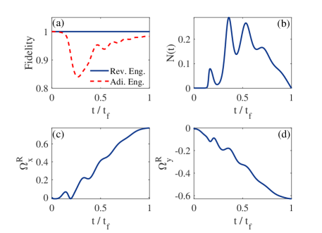
Figure 1: (a) The fidelity for the reverse engineering protocol (the blue solid line) and the adiabatic engineering protocol (the red dash line) vs the dimensionless time $t/t_{f}$. The control parameters ((b) the main excitation number $N$, (c) the coherent control field $\Omega^{\text{R}}_{x}$, and (d) the coherent control field $\Omega^{\text{R}}_{y}$) as a function of the dimensionless time $t/t_{f}$. Parameters: $\lambda=0.5\gamma_{0},\,\Delta=0.1\gamma_{0},\,\delta=0.5\gamma_{0},\,\Omega_{c}=10\gamma_{0},t_{f}=10/\gamma_{0}$, and $N_{0}=10^{-5}$. We set $\gamma_{0}=1$ as the unit of $\Omega^{\text{R}}_{x}$ and $\Omega^{\text{R}}_{y}$.

As shown in FIG.1 (a), the evolutions of the fidelities between the quantum state governed by the master equation Eq.(17) and the instantaneous steady state given by Eq.(41) are plotted for the inverse engineering protocol (blue solid line) and the adiabatic engineering protocol (red dash line). For the reverse engineering scheme, the quantum state of the open two-level system strictly follows the instantaneous steady state. When the adiabatic engineering protocol is used, i.e., $\Omega^{\text{R}}_{x}=\Omega^{\text{R}}_{0}$ and $\Omega^{\text{R}}_{y}=0$, the fidelity decrease evidently. Even the performance of the adiabatic engineering protocol is satisfied as long as the control time length $t_{f}$ increases,the quantum state deviates from the steady state trajectory at the intermediate time due to the rapid oscillation of the decay rate $\Gamma_{0}(t)$ and the Lamb shift $s_{0}(t)$.

The main excitation number $N(t)$ and the control field $\Omega^{\text{R}}_{x,y}(t)$ are also plotted in FIGs.1(b), (c) and (d). On the one hand, all of the control parametersoscillate with time, which is essential to offset effect of the rapid oscillation of the decay rate $\Gamma_{0}(t)$ and the Lamb shift $s_{0}(t)$. In this way, the quantum state is suppressed on the instantaneous steady state. On the other hand, due to the nonzero Lamb shift $s_{0}(t)$, the coherent control field $\Omega^{\text{R}}_{y}(t)$ is needed in the reverse engineering protocol, which does not appear in the reference Hamiltonian (or Liouvillian). If $s_{0}(t)=0$, the $x$-th component of the Bloch vector will be zero, which will result in the absence of coherent control field $\Omega^{\text{R}}_{y}(t)$ (see Eqs. (31) and (42)). This is the significant difference from the Markovian reverse engineering protocol counterpart.

III.2 The Population Inversion

Similar ideas can be applied to the population inversion of the two-level open quantum state. For convenience, we express the Bloch vector $\vec{r}$ by means of spherical polar coordinates, i.e.,

$$r_{x}=r\,\sin\theta\,\sin\phi,$$

$$r_{y}=r\,\cos\theta\,\sin\phi,$$

$$r_{z}=r\,\cos\phi.$$ (44)

Our aim is to transfer the quantum state from the ground state $|{0}\rangle$ into the excited state $|{1}\rangle$. $|{0}\rangle$ and $|{1}\rangle$ are the eigenvectors of $\sigma_{z}$. For that, we set the boundary conditions of quantum state as $\phi(0)=\pi$, $r(0)=1$, $\phi(t_{f})=0$, and $r(t_{f})=1$. It is free to choose the values of $\theta(0)$ and $\theta(t_{f})$. According to Eq.(31), when $\phi\rightarrow\pi/2$, the coherent control fields $\Omega^{\text{R}}_{x}$ and $\Omega^{\text{R}}_{y}$ tend to be infinite. In order to eliminate this singularity, we require $s_{0}=0$, $\dot{r}=0$ and $\dot{\theta}=0$ for $\phi=\pi/2$. Here we should mention that the requirement $s_{0}(t_{i})=0$ for some intermediate moment $t_{i}$ can be realized by picking a proper detuning $\Delta$. In addition, for the non-Markovian dynamics of open quantum systems, the decay rates are negative in some intermediate duration. Thus the main excitation $N(t)$ will be infinite at the moment for $\Gamma_{0}=0$. Yet, if we require $\vec{r}\cdot\dot{\vec{r}}=0$ at this point, a reasonable main excitation number can be obtained (see Eq.(31)).

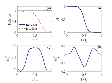
Figure 2: (a) The evolution of the fidelity of the reverse engineering protocol (the blue solid line) and the adiabatic engineering protocol (the red dash line). The control parameters ((b) the main excitation number $N$, (c) the coherent control field $\Omega^{\text{R}}_{x}$, and (d) the coherent control field $\Omega^{\text{R}}_{x}$) as a function of the dimensionless time $t/t_{f}$. Parameters: $\lambda=0.5\gamma_{0},\,\Delta=0.1\gamma_{0},\,\delta=0.5\gamma_{0},\,\Omega_{c}=10\gamma_{0},t_{f}=10/\gamma_{0}$ and $N_{0}=10^{-5}$. We set $\gamma_{0}=1$ as the unit of $\Omega^{\text{R}}_{x}$ and $\Omega^{\text{R}}_{y}$.

Firstly, we show that the population inversion with a pure-state trajectory is kinematically controllable, but not dynamically controllable. To interpolate at intermediate times, we consider a polynomial ansatz of $\theta$ and $\phi$ as a function of time $t$,

$$r(t) = 1,$$

$$\phi(t) = \pi\frac{t^{2}}{t_{f}^{2}}\left(3-2\frac{t}{t_{f}}\right),$$

$$\theta(t) = \theta\left(\frac{t_{f}}{2}\right)\frac{t^{2}}{t_{f}^{2}}\left(1-\frac{t}{t_{f}}\right)^{2},$$ (45)

with $\theta(0)=\theta(f_{f})=0$ and an arbitrary $\theta\left(\frac{t_{f}}{2}\right)$ at $t=t_{f}/2$. Under this ansatz, for $t=t_{f}/2$, we have $\phi(t_{f}/2)=\pi/2$ and $\dot{\theta}(t_{f}/2)=0$, which result in a reasonable coherent control fields in the control period. Figure 2 (a) shows the fidelities between the quantum state $\rho(t)$ and the preset trajectory given by Eq.(44) for the reverse engineering protocol (the blue solid line) and the inverse engineering protocol of closed quantum systems. The control parameters are plotted in FIG. 2 (b), (c) and (d). As we see, the reverse engineering protocol transfers the quantum state from $|{0}\rangle$ into $|{1}\rangle$ definitely, while the control parameters evolve smoothly. Therefore, the pure state protocol is kinematically controllable. But as shown in FIG. 2 (b), the main excitation number $N(t)$ is negative, which can not be feasible in experiment-setting, so that the reverse engineering protocol is not dynamically controllable for the pure-state trajectory.

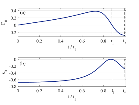
Figure 3: (a) The decay rate $\Gamma_{0}$ and (b) the Lamb shift vs the dimensionless time $t/t_{f}$, where $t_{f}$ is the control pulse length and $t_{i}$ is the moment where $r_{z}=0$. Parameters: $\lambda=0.1\gamma_{0},\,\Delta=-0.6792\gamma_{0},\,\delta=0.1\gamma_{0},\,\Omega_{c}=1\gamma_{0},t_{f}=9.1201/\gamma_{0}$. We set $\gamma_{0}=1$ as the unit of $\Gamma_{0}$ and $s_{0}$.

Secondly, we show that the population inversion is dynamically controllable if a mixed-state trajectory of the two-level non-Markovian system is carefully selected. As we see, the dynamical uncontrollability comes from the negative main excitation number. We can rewrite the main excitation number as

$$N(t)=-\left(\frac{1}{2}+\frac{{r_{z}}}{{r}^{2}+{r_{z}}^{2}}+\frac{\partial_{t}r^{2}}{4\Gamma_{0}\,\left({r}^{2}+{r_{z}}^{2}\right)}\right)$$ (46)

with the length of the Bloch vector $r=\sqrt{r_{x}^{2}+r_{y}^{2}+r_{z}^{2}}$. If the quantum state is pure, then $\partial_{t}r^{2}=0$ and $r=1$, which results in a negative main excitation number. The population inversion corresponds to the Bloch vector from $r_{z}(t)=-1$ to $r_{z}(t_{f})=1$. When $r_{z}$ varies from -1 to 0, the second term in Eq.(46) is negative. Moreover, if $r$ shortens with evolution, the third term in Eq.(46) is also negative. Thus, it can be ensured that the main excitation number is always positive in the lower hemisphere of the Bloch sphere. However, in the upper hemisphere of the Bloch sphere, i.e., $r_{z}>0$, the second term in Eq.(46) is positive, and $r$ needs to increase with time, so that the main excitation number can not be always positive in the evolution. However, the decay rate $\Gamma_{0}(t)$ is negative at some intermediate moment. Therefore, we propose following proposal to realize a dynamically controllable population inversion: (1). We set $t_{f}$ as the moment where $\Gamma_{0}$ reaches the negative maximum for the first time, and label $t_{i}$ as the moment when $\Gamma_{0}(t_{i})=0$ for $t_{i}\in(0,t_{f})$, which is illustrated in FIG. 3 (a). (2). Since $\Gamma_{0}(t)>0$ for $t\in(0,t_{i})$, we impose that $r_{z}(t_{i})=0$ and $r_{z}(t)<0$ for $t<t_{i}$. In this way, it is easy to present a positive main excitation number for $t<t_{i}$ by selecting a mixed trajectory. (3). Since $\Gamma_{0}(t)<0$ for $t\in(t_{i},t_{f})$, the third term in Eq.(46) will be negative if $r^{2}$ keeps increasing. Thus it is possible to present a positive the main excitation number if $\vec{r}(t)\cdot\dot{\vec{r}}(t)$ increases fast enough.

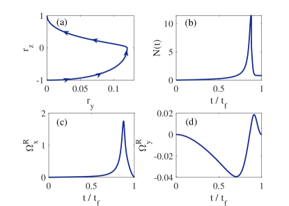
Figure 4: (a) The evolution of quantum state trajectory in the Bloch sphere as a function of the dimensionless time $t/t_{f}$. (b) The main excitation number $N$, (c) the coherent control field $\Omega^{\text{R}}_{x}$ and (d) the coherent control field $\Omega^{\text{R}}_{y}$ as a function of the dimensionless time $t/t_{f}$. Parameters: $\lambda=0.1\gamma_{0},\,\Delta=-0.6792\gamma_{0},\,\delta=0.1\gamma_{0},\,\Omega_{c}=1\gamma_{0},t_{f}=9.1201/\gamma_{0}$. We set $\gamma_{0}=1$ as the unit of $\Omega^{\text{R}}_{x}$ and $\Omega^{\text{R}}_{y}$.

As an example, we impose the boundary conditions of components of the Bloch vector as follows,

$$\begin{array}[]{ccc}r_{y}(0)=0,&r_{y}(t_{i})=0.12,&r_{y}(t_{f})=0;\\ \dot{r}_{y}(0)=0,&\dot{r}_{y}(t_{i})=0,&\dot{r}_{y}(t_{f})=0;\\ r_{z}(0)=-1,&r_{z}(t_{i})=0,&r_{z}(t_{f})=1;\\ \dot{r}_{z}(0)=0,&\dot{r}_{z}(t_{i})=0.4,&\dot{r}_{z}(t_{f})=1;\\ \end{array}$$ (51)

and $r_{x}(t)=0$ for $\forall t$. The reason why we selected the boundary conditions as Eq.(51) is to eliminate the singular points in the control parameters and obtain the positive main excitation number. As shown in Eq.(31), $\Omega^{\text{R}}_{x}$ and $\Omega^{\text{R}}_{y}$ have singular points at $t=t_{i}$ because of $r_{z}(t_{i})=0$. Thus, we require $\dot{r}_{x}(t_{i})=\dot{r}_{y}(t_{i})=0$, and further impose $s_{0}(t_{i})=0$ which is illustrated in FIG. 3 (b). On the other hand, if $\vec{r}\cdot\dot{\vec{r}}>-\Gamma_{0}r_{z}(r_{z}+1)$, $N$ will be positive. For $t=t_{i}$, the positive main excitation number requires $\dot{r}_{z}(t_{i})>-\Gamma_{0}(t_{i})$. Thus, the time derivative of $r_{z}(t_{i})$ must be nonzero and finite positive number. Due to $r_{z}(t_{i})=\dot{r}_{y}(t_{i})=0$, it is not difficult to verify that $\vec{r}\cdot\dot{\vec{r}}=0$, so that the singular point in Eq.(46) is also eliminated. At last, the time derivative of $r_{z}(t_{f})$ must be nonzero and finite positive number, which results in $N(t_{f})>0$ (see Eq.(46)). To interpolate at intermediate times, we assume a polynomial ansatz and consider a piecewise interpolation with a time break $t_{i}$. Figure 4 (a) shows the numerical results of the quantum state trajectory in the Bloch sphere, which illustrates that the population is transferred from $|{0}\rangle$ into $|{1}\rangle$ completely. The main excitation number $N$, the coherent control fields $\Omega^{\text{R}}_{x}$ and $\Omega^{\text{R}}_{y}$ are plotted in FIG.4 (b), (c) and (d), respectively. As shown in those figures, the control parameters with the boundary conditions of the trajectory Eq.(51) are reasonable, which can be realized in experimental-settings. Therefore, the population inversion for the two-level non-Markovian system is dynamical controllable definitely.

IV Conclusions and Discussions

In conclusion, based on the idea of reverse engineering, we have proposed a scheme to transfer the quantum state of non-Markovian systems along a designable trajectory in the Hilbert space strictly. For the quantum systems are governed by a time-convolutionless master equation, we have presented the analytical expressions of control parameters, which are the solution of algebraic equations with quantum state trajectories. Even though the open quantum system suffers the memory effects of the non-Markovian reservoir (the information backflow or/and the Lamb shift), the quantum state can still transfer into the target state along designed trajectory strictly. Taking the driven non-Markovian two-level system as an example, we present concrete control protocol for both the instantaneous steady state tracking and the population inversion. By elaborately designing the trajectory of the quantum state, it has been shown that the non-Markovian two-level system is not only kinematically controllable, but also dynamically controllable. Since the scheme allows us to maintain system coherence and populations in the presence of noises, it may naturally find applications in quantum computing and quantum memories Kang2020 ; Shi2020 . Our scheme can also be applied to numerous quantum control problems, such as the quantum state preparing Wu2015 , the quantum measurement Zheng2020 , and the quantum metrology.

It is meaningful to compare our scheme with the reverse engineering scheme of the Markovian quantum systems ran2020 ; medina2019 . For the Markovian quantum systems, it shows that the quantum state is not dynamically controllable Wu2007 ; Koch2016 . For instance, the complete population inversion of two-level systems can not be realized in the experimental-setting. The population of the excited state is only asymptotically getting closer to 1, which is discussed in the example of the population inversion ran2020 . Due to the information which can flow back into the open two-level systems bylicka2017 ; guarnieri2016 , the complete population inversion for the non-Markovian dynamics can be realized by carefully designing the trajectory of the quantum state sweeping in the Hilbert space. In other words, the non-Markovianity will benefit the quantum control process.

This work is supported by National Natural Science Foundation of China (NSFC) under Grants No. 12075050 and 11775048.

Appendix A The Derivation of Eq.(9)

We begin with the time-convolutionless master equation in the superoperator form Eq.(4). Taking the density operator vector Eq.(6) into Eq.(4)Schirmer2010 , it yields

$$\partial_{t}r_{i}(t)=\sum_{j=1}^{N^{2}-1}\mathcal{L}_{ij}r_{j}+\mathcal{L}^{0}_{i},$$ (52)

where the Liouvillian superoperator can be written in the supermatrix form

$$\hat{\mathcal{L}}=\sum_{ij=1}^{N^{2}-1}\mathcal{L}_{i,j}|T_{i}\rangle\rangle\langle\langle T_{j}|+\sum_{i=1}^{N^{2}-1}\mathcal{L}^{0}_{i}|T_{i}\rangle\rangle\langle\langle T_{0}|,$$ (53)

with $\mathcal{L}_{ij}(t)=\text{Tr}[T_{i}^{\dagger}(\hat{\mathcal{L}}[T_{j}])]$ and $\mathcal{L}_{i}^{0}(t)=\text{Tr}[T_{i}^{\dagger}(\hat{\mathcal{L}}[T_{0}])]$. Here, the relation $\hat{\mathcal{L}}^{\dagger}(t)|T_{0}\rangle\rangle=\langle\langle T_{0}|\hat{\mathcal{L}}(t)=0$ has been used. We divide Liouvillian supermatrix into two parts $\mathcal{L}_{ij}=\mathcal{C}_{ij}+\mathcal{I}_{ij}$ , where $\mathcal{I}_{ij}$ ($\mathcal{C}_{ij}$) denotes the incoherent (coherent) part of the Liouvillian supermatrix element $\mathcal{L}_{ij}$.

The coherent part comes from the Hamiltonian part in the master equation

$$\mathcal{C}_{ij}=-i\>\text{Tr}\left[T_{i}^{\dagger}\,[H(t),T_{j}]\right].$$ (54)

By substituting Eq.(7) into above equation, we have

$$\mathcal{C}_{ij}=-i\>\sum_{k=0}^{N^{2}-1}c_{k}(t)\,\text{Tr}\left[T_{i}\,[T_{k},T_{j}]\right].$$ (55)

Considering the commutator and anti-commutator of the SU($N$) generators

$$[T_{k},T_{j}] = i\sum_{m=1}^{N^{2-1}}f_{kjm}T_{m},$$ (56)

$$\left\{T_{k},T_{j}\right\} = \frac{\delta_{kj}}{N}\,I+\sum_{m=1}^{N^{2}-1}d_{kjm}\,T_{m},$$ (57)

we obtain the coherent part in the Liouvillian supermatrix

$$\mathcal{C}_{ij} = \sum_{k=1}^{N^{2}-1}\sum_{m=1}^{N^{2-1}}f_{kjm}c_{k}(t)\,\text{Tr}[T_{i}T_{m}]$$ (58)

$$= \sum_{k=1}^{N^{2}-1}\frac{f_{kji}}{2}c_{k}(t),$$

where $f_{ijk}$ and $d_{ijk}$ are the structure constants and the d-coefficients of the SU($N$) Lie algebra, respectively.

For the incoherent part, it can be expressed as

$$\mathcal{I}_{ij}=\text{Tr}\left[T_{i}^{\dagger}\sum_{\alpha}\gamma_{\alpha}\left(2L_{\alpha}T_{j}L_{\alpha}^{\dagger}-\left\{L_{\alpha}^{\dagger}L_{\alpha},T_{j}\right\}\right)\right].$$ (59)

The Lindblad operators can also be expanded by the SU($N$) Hermitian generators $\{T_{i}\}_{i=1}^{N^{2}-1}$, i.e

$$L_{\alpha}(t)=\sum_{j=1}^{N^{2}-1}l_{j}^{(\alpha)}(t)\,T_{j}$$ (60)

with complex coefficients $l_{j}^{(\alpha)}(t)$ , and

$$L_{\alpha}^{\dagger}(t)=\sum_{j=1}^{N^{2}-1}l_{j}^{(\alpha)*}(t)\,T_{j},$$

$$L_{\alpha}^{\dagger}(t)L_{\alpha}(t)=\sum_{i=0}^{N^{2}-1}e_{k}^{(\alpha)}(t)\,T_{k},$$ (61)

with $e_{n}^{(\alpha)}=\frac{1}{2}\sum_{i,j=0}^{N^{2}-1}l_{i}^{(\alpha)}(t)l_{j}^{(\alpha)*}(t)\,\left(i\,f_{ijn}+d_{ijn}\right)$ for $n\neq 0$ and $e_{0}^{(\alpha)}=\sum_{i=0}^{N^{2}-1}\frac{\left|l_{i}^{(\alpha)}(t)\right|^{2}}{2N}$. Thus, it is easy to obtain

$$\text{Tr}\left[T_{i}^{\dagger}\left\{L_{\alpha}^{\dagger}L_{\alpha},T_{j}\right\}\right]=e_{0}^{(\alpha)}\,\delta_{ij}+\sum_{k=1}^{N^{2}-1}\frac{d_{kji}}{2}\,e_{k}^{(\alpha)},$$

$$\text{Tr}\left[T_{i}^{\dagger}L_{\alpha}T_{j}L_{\alpha}^{\dagger}\right]=\frac{l_{i}^{(\alpha)}l_{j}^{(\alpha)*}}{4N}+h_{ji}^{(\alpha)},$$ (62)

with

$$h_{ji}^{(\alpha)}=\frac{1}{8}\sum_{p=1}^{N^{2}-1}\sum_{m,n=0}^{N^{2}-1}l_{m}^{(\alpha)}l_{n}^{(\alpha)*}\left(i\,f_{jnp}+d_{jnp}\right)\left(i\,f_{imp}+d_{imp}\right).$$

Rearranging equations, we finally obtain the incoherent part of the Liouvillian supermatrix

$$\mathcal{I}_{ij}=\sum_{m,n=0}^{N^{2}-1}\left(\sum_{\alpha}\gamma_{\alpha}l_{m}^{(\alpha)}(t)l_{n}^{(\alpha)*}(t)\right)s_{mn,ji},$$ (63)

with

$$s_{mn,ji} = \frac{1}{2N}\left(\delta_{im}\,\delta_{jn}-\delta_{mn}\,\delta_{ij}\right)$$ (64)

$$+\frac{1}{4}\sum_{k=1}^{N^{2}-1}\left(\left(i\,f_{jnk}+d_{jnk}\right)\left(i\,f_{imk}+d_{imk}\right)\right.$$

$$\left.-\left(i\,f_{mnk}+d_{mnk}\right)\,d_{kji}\right),$$

where $|l_{m}^{(\alpha)}(t)|^{2}=\sum_{n}l_{m}^{(\alpha)}(t)l_{n}^{(\alpha)*}(t)\delta_{mn}$ has been used.

The last term in Eq.(52) originates from the expansion of $\mathcal{L}$ with the basis $|T_{i}\rangle\rangle\langle\langle T_{0}|$. For $j=0$, this term can be written as

$$\mathcal{L}_{k}^{0}(t) = 2\text{Tr}\left[T_{k}^{\dagger}\sum_{\alpha}\gamma_{\alpha}(t)\left(L_{\alpha}(t)L_{\alpha}^{\dagger}(t)-L_{\alpha}^{\dagger}(t)L_{\alpha}(t)\right)\right]$$ (65)

$$= \sum_{\alpha}\gamma_{\alpha}(t)\left(\sum_{i,j=1}^{N^{2}-1}l_{i}^{(\alpha)}(t)l_{j}^{(\alpha)*}(t)\right.$$

$$\left.\times\left(\left(i\,f_{jik}+d_{jik}\right)-\left(i\,f_{ijk}+d_{ijk}\right)\right)\right)$$

Appendix B A control protocol without $\Omega^{R}_{y}$

We also consider a two-level system used in Sec. III, whose dynamics is governed by the non-Markovian master equation Eq.(17). Here, we consider the renormalized control field is real and there is a detuning $\Delta^{\text{R}}$ to the two-level system. Thus, the Hamiltonian in Eq.(17) can be written as

$$H_{s}^{\text{R}}(t)=s_{0}(t)\sigma_{+}\sigma_{-}+\Delta^{\text{R}}(t)\sigma_{z}+\Omega^{\text{R}}_{x}(t)\sigma_{x}.$$ (66)

We still assume that the spectrum density is untunable in experimental-settings. At this time, the coherent control parameters are $\Omega^{\text{R}}_{x}(t)$ and $\Delta^{\text{R}}(t)$, while the main excited number $N(t)$ acts as the incoherent control parameter. Taking the control parameters and the components of the Bloch vector into Eq.(13), it yields

$$\mathrm{\dot{r}_{x}} = -(s_{0}+\Delta^{\text{R}})\,\mathrm{r_{y}}-\left(2\,N+1\right)\,\Gamma_{0}\,\mathrm{r_{x}},$$

$$\mathrm{\dot{r}_{y}} = (s_{0}+\Delta^{\text{R}})\,\mathrm{r_{x}}-\left(2\,N+1\right)\,\Gamma_{0}\,\mathrm{r_{y}},$$

$$\mathrm{\dot{r}_{z}} = 2\,\mathrm{\Omega_{x}^{\text{R}}}\,\mathrm{r_{y}}-2\,\Gamma_{0}\,\left(\left(2\,N+1\right)\,\mathrm{r_{z}}+1\right)\!\!.$$ (67)

We can reversely solve Eq.(67), and obtain

$$\Omega_{x}^{\text{R}} = \frac{\left(2\,\Gamma_{0}+\partial_{t}r_{z}\right)\,\left(r_{x}^{2}+r_{y}^{2}\right)-\partial_{t}\left(r_{x}^{2}+r_{y}^{2}\right)\,r_{z}}{2\,\mathrm{r_{y}}\,\left(\mathrm{r}^{2}+\mathrm{r_{z}}^{2}\right)},$$

$$\Delta^{\text{R}} = -s_{0}+\frac{r_{x}\,\left(r_{y}\dot{r}_{y}+r_{z}\dot{r}_{z}\right)+2\,\Gamma_{0}\,r_{x}r_{z}-\dot{r}_{x}\,\left(r_{y}^{2}+2\,r_{z}^{2}\right)}{\mathrm{r_{y}}\,\left(\mathrm{r_{x}}^{2}+\mathrm{r_{y}}^{2}+2\,\mathrm{r_{z}}^{2}\right)},$$

$$N = -\frac{2\,\Gamma_{0}\,\mathrm{r_{z}}+\vec{\mathrm{r}}\cdot\dot{\vec{\mathrm{r}}}+\mathrm{\Gamma_{0}}\,\left(\mathrm{r}^{2}+\mathrm{r_{z}}^{2}\right)}{2\,\mathrm{\Gamma_{0}}\,\left(\mathrm{r}^{2}+\mathrm{r_{z}}^{2}\right)}.$$ (68)

Thus, we obtain a control protocol without $\Omega^{\text{R}}_{y}$. This protocol has advantages in the population reversion task, because the singular points of control parameters only appear at $r_{y}=0$. We may design the trajectory of quantum state away from points with $r_{y}=0$. For the completely population reversion, the initial and final state require $r_{y}=0$. However, we can set proper boundary conditions for $r_{i}$ and $\dot{r}_{i}$ to eliminate those singular points.

References

- (1) C. P. Koch, M. Lemeshko, and D. Sugny, Rev. Mod. Phys. 91, 035005 (2019).
- (2) S. Osnaghi, P. Bertet, A. Auffeves, P. Maioli, M. Brune, J. M. Raimond, and S. Haroche, Phys. Rev. Lett. 87, 037902 (2001).
- (3) S. Hacohen-Gourgy, L. P. García-Pintos, L. S. Martin, J. Dressel, and I. Siddiqi, Phys. Rev. Lett. 120, 020505 (2018).
- (4) L. C. Venuti, T. Albash, M. Marvian, D. Lidar, and P. Zanardi, Phys. Rev. A 95, 042302 (2017).
- (5) R. Dann, A. Tobalina, and R. Kosloff, Phys. Rev. Lett. 122, 250402 (2019).
- (6) S. Zippilli and D. Vitali, Phys. Rev. Lett. 126, 020402 (2021).
- (7) R. H. Zheng, Y. Xiao, S. L. Su, Y. H. Chen, Z. C. Shi, J. Song, Y. Xia, and S. B. Zheng, Phys. Rev. A 103, 052402 (2021)
- (8) S. L. Wu, W. Ma, X. L. Huang, and X. X. Yi, arXiv: 2103.12336.
- (9) F. Liu, X. Zhou, and Z. W. Zhou, Phys. Rev. A 99, 052119 (2019).
- (10) W. M. Zhang, P. Y. Lo, H. N. Xiong, Matisse Wei-Yuan Tu, and F. Nori, Phys. Rev. Lett. 109, 170402 (2012).
- (11) L. Li, M. J. Hall, and H. M. Wiseman, Phys. Rep. 759, 1 (2018).
- (12) G. Gasbarri and L. Ferialdi, Phys. Rev. A 97, 022114 (2018).
- (13) M. R. Jørgensen and F. A. Pollock, Phys. Rev. A 102, 052206 (2020).
- (14) I. de Vega and D. Alonso, Rev. Mod. Phys. 89, 015001 (2017).
- (15) A. Pereverzev and E. R. Bittner, J. Chem. Phys. 125, 104906 (2006).
- (16) F. Minganti, A. Biella, N. Bartolo, and C. Ciuti, Phys. Rev. A 98, 042118 (2018).
- (17) D. Basilewitsch, F. Cosco, N. L. Gullo, M. Möttönen, T. Ala-Nissilä, C. P. Koch, and S. Maniscalco, New J. Phys. 21, 093054 (2019).
- (18) A. Shabani and H. Neven, Phys. Rev. A 94, 052301 (2016).
- (19) K. Seetharam, A. Lerose, R. Fazio, and J. Marino, arXiv preprint arXiv:2101.06445 (2021).
- (20) A. Pechen and H. Rabitz, Phys. Rev. A 73, 062102 (2006).
- (21) S. Alipour, A. Chenu, A. T. Rezakhani, and A. del Campo, Quantum 4, 336 (2020).
- (22) X. Chen, I. Lizuain, A. Ruschhaupt, D. Guéry-Odelin, and J. G. Muga, Phys. Rev. Lett. 105, 123003 (2010).
- (23) R. Wu, A. Pechen, C. Brif, and H. Rabitz, J. Phys. A 40, 5681 (2007).
- (24) A. Grigoriu, H. Rabitz, and G. Turinici, J. Math. Chem. 51, 1548 (2013).
- (25) M. Lostaglio, K. Korzekwa, and A. Milne, Phys. Rev. A 96, 032109 (2017).
- (26) B. Buča and T. Prosen, New Journal of Physics 14, 073007 (2012).
- (27) H. Z. Shen, M. Qin, X. M. Xiu, and X. X. Yi, Phys. Rev. A 89, 062113 (2014).
- (28) W. Cui, Z. R. Xi, and Y. Pan, Phys. Rev. A 77, 032117 (2008).
- (29) H. Z. Shen, M. Qin, and X. X. Yi, Phys. Rev. A 88, 033835 (2013).
- (30) P. Haikka and S. Maniscalco, Phys. Rev. A 81, 052103 (2010).
- (31) D. Ran, W. J. Shan, Z. C. Shi, Z. B. Yang, J. Song, and Y. Xia, Phys. Rev. A 101, 023822 (2020).
- (32) K. Hornberger, Phys. Rev. Lett. 97, 060601 (2006).
- (33) C. P. Koch, Journal of Physics: Condensed Matter 28, 213001 (2016).
- (34) S. L. Wu, X. L. Huang, X. X. Yi, Phys. Rev. A 99, 042115 (2019).
- (35) V. Cavina, A. Mari, and V. Giovannetti, Phys. Rev. Lett. 119, 050601 (2017).
- (36) J. Anders and M. Esposito, New J. Phys. 19, 21 (2017).
- (37) H. J. D. Miller, M. H. Mohammady, M. Perarnau-Llobet, and G. Guarnieri, Phys. Rev. Lett. 126, 210603 (2021).
- (38) S. H. Raja, S. Maniscalco, G. S. Paraoanu, J. P. Pekola, and N. L. Gullo, New J. Phys. 23, 033034 (2021).
- (39) Y. H. Kang, Z. C. Shi, B. H. Huang, J. Song, and Y. Xia, Phys. Rev. A 101, 032322 (2020).
- (40) Z. C. Shi, C. Zhang, L. T. Shen, Y. Xia, X. X. Yi, and S. B. Zheng, Phys. Rev. A 101, 042314 (2020).
- (41) S. L. Wu, Phys. Rev. A 91, 032104 (2015).
- (42) R. H. Zheng, Y. H. Kang, S. L. Su, J. Song, and Y. Xia, Phys. Rev. A 102, 012609 (2020).
- (43) I. Medina and F. L. Semiao, Phys. Rev. A 100, 012103 (2019).
- (44) B. Bylicka, M. Johansson, and A. Acín, Phys. Rev. Lett. 118, 120501 (2017).
- (45) G. Guarnieri, C. Uchiyama, and B. Vacchini, Phys. Rev. A 93, 012118 (2016).
- (46) S. G. Schirmer, X. Wang, Phys. Rev. A 81, 062306 (2010).