Experimental secure quantum key distribution in presence of polarization-dependent loss

Abstract

Quantum key distribution (QKD) is theoretically secure using the principle of quantum mechanics; therefore, QKD is a promising solution for the future of secure communication. Although several experimental demonstrations of QKD have been reported, they have not considered the polarization-dependent loss in state preparation in the key-rate estimation. In this study, we experimentally characterized polarization-dependent loss in realistic state-preparation devices and verified that a considerable PDL exists in fiber- and silicon-based polarization modulators. Hence, the security of such QKD systems is compromised because of the secure key rate overestimation. Furthermore, we report a decoy-state BB84 QKD experiment considering polarization-dependent loss. Finally, we achieved rigorous finite-key security bound over up to 75 km fiber links by applying a recently proposed security proof. This study considers more realistic source flaws than most previous experiments; thus, it is crucial toward a secure QKD with imperfect practical devices.

I introduction

Quantum key distribution (QKD) has received great interest as it is an information-theoretic security communication technology Lo and Chau (1999). With much effort, QKD has been experimentally demonstrated over fiber-based Choi et al. (2016); Cañas et al. (2017); Boaron et al. (2018); Liu et al. (2010); Wang et al. (2012); Ma et al. (2021); Zhou et al. (2021); Bunandar et al. (2018), free-space Liao et al. (2017); Chen et al. (2020); Avesani et al. (2021), and underwater channels Hu et al. (2019). Various quantum field networks have been reported worldwide Chen et al. (2010); Sasaki et al. (2011); Wang et al. (2014); Dynes et al. (2019); Yang et al. (2021). Interestingly, an integrated space-to-ground quantum network, based on a trusted-relay structure enabling multi-user secure communication over a total distance of 4600 km, was recently implemented Chen et al. (2021a). Even more recently, the record-breaking distances of QKD have been pushed to 511 km for field-deployed fiber Chen et al. (2021b) and 605 km for fiber spool Pittaluga et al. (2021) based on an efficient version of a measurement-device-independent QKD protocol Lo et al. (2012) called twin-field QKD Lucamarini et al. (2018); Ma et al. (2018); Wang et al. (2018, 2019).

The security of QKD is provided by the principle of quantum physics, assuming that the features of real-life components conform to the theoretical models in the security proof Gottesman et al. (2004). However, existing imperfections in practical implementations break these ideal assumptions, leaving several considerable vulnerabilities to eavesdropping by Eve. Indeed, multiple quantum hacking attacks Qian et al. (2018); Yoshino et al. (2018); Wei et al. (2019); Huang et al. (2020); Pang et al. (2020) have been proposed by exploiting such realistic security loopholes (see Xu et al. (2020) for a recent review on this topic).

In the current security proofs of QKD, a fundamental assumption is that the intensity of a quantum signal is not relate to its actual encoded state Gottesman et al. (2004). The goal is to prevent Eve from learning the encoded bit by performing an unambiguous state discrimination attack Tang et al. (2013). Unfortunately, this key assumption cannot be guaranteed by state-of-the-art polarization-encoding modulators, which are mainly integrated using several fiber or silicon photonics components. This is because almost all of the above optical components, arising from physical structures, inevitably have some amount of polarization-dependent loss (PDL). For instance, according to Ref. Sibson et al. (2017), the PDL due to carrier-depletion modulators was approximately 1 dB.

In this study, we experimentally characterized PDL in realistic polarization state preparation schemes and verified that PDL exists in fiber- Agnesi et al. (2019); Li et al. (2019) and silicon-based polarization modulators (PMs) Wei et al. (2020). Furthermore, we report a decoy-state BB84 QKD experiment that considers the PDL. Our demonstration exploits a novel theoretical proposal of Li et al. Li et al. (2018), which enables long-distance QKD through the post-selection of signals. We call this proposal a polarization-loss-tolerant protocol. With the refined security proof, we successfully distributed secure key bits over different fiber links up to a 75 km. In contrast, no secure key bits can be generated using standard Gottesman-Lo-Lütkenhaus-Preskill (GLLP) analysis Gottesman et al. (2004). The theoretical and experimental contributions are detailed below.

Theoretically, we combine the one-decoy-state method with the polarization-loss-tolerant protocol. This can significantly simplify the experimental complexity of the polarization-loss-tolerant protocol. Note that the one-decoy-state method has recently been proven to outperform the two-decoy-state method for almost all experimental settings, and only one decoy is easier to implement  Rusca et al. (2018). Thus, our analysis is crucial for implementing a polarization-loss-tolerant protocol and ensuring the security of practical QKD existing in the PDL. In addition, we quantify the security of QKD systems in the presence of PDL using a standard GLLP approach. This provides a quantitative observation for relating the security to specific values of PDL in PM.

Experimentally, we verified that PDL exists in recently proposed fiber- and silicon-based polarization modulation schemes. Furthermore, we performed the first decoy-state BB84 QKD demonstration using a homemade QKD system by considering the PDL. We quantified the PDL in state-preparation devices and considered it into the key rate formula. Using the polarization-loss-tolerant protocol, we successfully distributed secure key bits over up to 75 km of commercial fiber spool.

The remainder of this paper is as follows. In Sec. II, we present the one-decoy-state polarization-loss-tolerant protocol. In Sec. III, we describe our experimental setup and present the experimental results. Finally, we summarize our work in Sec. IV.

II Polarization-loss-tolerant protocol with one-decoy-state method

II.1 Original protocol

The key idea of the polarization-loss-tolerant protocol is that the photons unbalanced by the PDL can be randomly discarded. Hence, the final secret key is only extracted from the single-photon components whose density matrices are maximally mixed Li et al. (2018). In this manner, the destroyed assumption due to the PDL is restored. Furthermore, a post-selection scheme is introduced to reduce the consumption of error correction, and a higher secret key rate is obtained. With the refined security proof in the polarization-loss-tolerant protocol, the final secret key bits can be given as

$$R\geqslant q\left\{-\hat{Q}_{\mu}f\left(\hat{E}_{\mu}\right)H\left(\hat{E}_{\mu}\right)+\hat{Q}_{1}\left[1-H\left(e_{1}^{ph}\right)\right]\right\},$$ (1)

where $q$ is the efficiency of the protocol, $\hat{Q}_{1}$ and $e_{1}^{ph}$ are the gain and phase error rate of the single-photon states, respectively, $\hat{Q}_{\mu}$ and $\hat{E}_{\mu}$ denote the gain and overall QBER of the signal states, respectively, $f(\hat{E}_{\mu})$ is the efficiency of error correction, and $H(x)$ is the binary Shannon entropy.

The parameters required in Eq. (1) can be estimated using the decoy-state technique Wang (2005); Lo et al. (2005) for different polarizations, which can be summarized as

$$\hat{Q}_{1} =\min\left\{P\times\mu_{H}e^{-\mu_{H}},\mu_{V}e^{-\mu_{V}}\right\}\times Y_{1},$$ (2)

$$Y_{1} =\frac{Y_{1,H}+Y_{1,V}}{2},$$

$$e_{1}^{ph} =\frac{Y_{1,D}e_{1,D}+Y_{1,A}e_{1,A}}{Y_{1,D}+Y_{1,A}},$$

$$\hat{Q}_{\mu} =\frac{P\times Q_{\mu_{H}}+Q_{\mu_{V}}}{2},$$

$$\hat{Q}_{\mu}\hat{E}_{\mu} =\frac{P\times Q_{\mu_{H}}E_{\mu_{H}}+Q_{\mu_{V}}E_{\mu_{V}}}{2},$$

where $\mu_{M}$ with $M\in\{H,~{}V,~{}D,~{}A\}$ represent the intensities of the signal state prepared in a given polarization $M$. $P$ is the post-selection probability to compensate the single-photon components loss of the V base, given by $\mu_{V}e^{-\mu_{V}}=P\times\mu_{H}e^{-\mu_{H}}$. $Y_{1,M}$ and $e_{1,M}$ denote the yield and QBER of the single-photon state prepared in the given polarization $M$, respectively. Moreover, $Q_{\mu_{M}}$ and $E_{\mu_{M}}$ are the gain and QBER of the signal states prepared in the given polarization $M$, respectively.

II.2 Parameter estimation using one-decoy-state method

In Ref. Li et al. (2018), the parameters required in Eq. (1) were estimated using the two-decoy-state method, which has a relatively complex implementation. Here, we used the one-decoy-state method Rusca et al. (2018) for parameter estimation, which significantly reduced the experimental complexity. Based on the framework presented in Rusca et al. (2018), the final secure key is given by

$$l\geqslant s_{z,0}^{L}+s_{z,1}^{L}(1-h\left(e_{z,1}^{ph}\right))$$ (3)

$$-leak_{EC}-6\log_{2}\frac{19}{\varepsilon_{sec}}-\log_{2}\frac{2}{\varepsilon_{cor}},$$

where $s_{z,0}^{L}$ is the lower bound of the detection counts by Bob given that Alice sent the vacuum pulses in the $z$ basis, $s_{z,1}^{L}$ is the analytical lower bound of the single-photon pulses in the $z$ basis, and $e_{z}^{ph}$ is the phase error rate. $leak_{EC}$ is the number of announced bits in the error correction stage, and $\varepsilon_{sec}$ and $\varepsilon_{cor}$ are the secrecy and correctness criteria, respectively.

Table 1: Concrete descriptions for one-decoy-state polarization-loss-tolerant protocol.

$Definitions:$

$\lambda:$ basis choice, $\lambda\in\{z,x\}$.

$k:$ intensity choice for signal and decoy state, $k\in\{\mu,\nu\}$.

$M:$ polarization choice, $M\in\{H,V,D,A\}$.

$k_{M}:$ intensity choice for given polarization $M$.

$p_{\lambda}:$ probability choice for basis $\lambda$, $p_{\lambda}\in\{p_{z},(1-p_{z})\}$.

$p_{k}:$ probability choice for intensity $k$, $p_{k}\in\{p_{\mu},p_{\nu}\}$.

$P_{k}:$ post-selection probability choice for intensity $k$, $P_{k}\in\{P_{\mu},P_{\nu}\}$.

$L_{\lambda}:$ polarization-dependent loss coefficient for basis $\lambda$.

$Measured\quad quantities:$

$n_{z}:$ total number of detected pulses when Alice sends states in basis $z$ .

$n_{\lambda,k_{M}}:$ number of detected pulses when Alice sends states in basis $\lambda$ and polarization $M$ with intensity $k$.

$m_{\lambda,k_{M}}:$ number of error pulses when Alice sends states in basis $\lambda$ and polarization $M$ with intensity $k$.

$Statistical\quad fluctuations:$

$\delta:$ statistics, $\delta\left(\chi,\varepsilon\right):=\sqrt{\chi\log\left(1/\varepsilon\right)/2}$.

$n_{\lambda,k_{M}}^{\pm}:$ upper and lower bounds of $n_{\lambda,k_{M}}$, $n_{\lambda,k_{M}}^{\pm}=n_{\lambda,k_{M}}\pm\delta\left(n_{\lambda},\varepsilon_{1}\right)$.

$m_{\lambda,k_{M}}^{\pm}:$ upper and lower bounds of $m_{\lambda,k_{M}}$, $m_{\lambda,k_{M}}^{\pm}=m_{\lambda,k_{M}}\pm\delta\left(m_{\lambda},\varepsilon_{2}\right)$.

$\tau_{n,M}:$ $n$-photon-state probability for polarization $M$, $\tau_{n,M}=\sum_{k\in_{\mu,\nu}}p_{k}e^{-k_{M}}k_{M}^{n}/n!$.

$Decoy-estimation\quad results:$

$s_{z,0}^{L}:$ lower bound of vacuum events in basis $z$ according to Eq. (7).

$s_{z,1}^{L}:$ lower bound of single-photon events in basis $z$ according to Eq. (8).

$e_{z}^{ph}:$ phase error rate in the $Z$ basis according to Eq. (9).

Due to the presence of the PDL, according to Eq. (2), $\{s_{z,0}^{L},s_{z,1}^{L},e_{z}^{ph}\}$ can be estimated from the measured quantities for different polarizations. In detail, let $s_{\lambda,n,M}$ be the number of detection counts measured by Bob given that Alice prepares $n$-photon states in basis $\lambda\in\{z,x\}$ and polarization $M$. In the asymptotic case, we obtained the number of detected pulses when Alice sends states in basis $\lambda$ and polarization $M$ with intensity $k\in\{\mu,\nu\}$ as

$$n_{\lambda,k_{M}}^{*}=\sum_{n=0}^{\infty}p_{{k_{M}}|n}s_{\lambda,n,M},$$ (4)

where $p_{{k_{M}}|n}=\frac{p_{k}}{\tau_{n,M}}\frac{e^{-k_{M}}k_{M}^{n}}{n!}$ is the conditional probability of selecting intensity $k$ provided that Alice prepares an $n$-photon pulse in polarization $M$, and the subscript $*$ denotes the presence of an asymptotic case. Furthermore, $\tau_{n,M}=\sum_{k\in_{\mu,\nu}}p_{k}e^{-k_{M}}k_{M}^{n}/n!$ is the probability that Alice prepares an $n$-photon pulse for polarization $M$, where $k_{M}$ represents the intensity of the state prepared in a particular polarization $M$. Correspondingly, let $v_{\lambda,n}$ be the number of errors detected by Bob when Alice sends an $n$-photon pulse and $m_{\lambda}=\sum_{n=0}^{\infty}v_{\lambda,n}$ is the total number of errors in the $\lambda$ basis. In the asymptotic case corresponding to different polarizations, the number of error pulses when Alice sends states in basis $\lambda$ and polarization $M$ with intensity $k$ can be obtained as

$$m_{\lambda,k_{M}}^{*}=\sum_{n=0}^{\infty}p_{{k_{M}}|n}v_{\lambda,n,M}.$$ (5)

Here, we adopt the observed counts in the $z$ basis to distill the secret key. When Alice sends $n$-photon pulses in $z$ basis, $n_{z}=\sum_{n=0}^{\infty}(s_{z,n,H}+s_{z,n,V})$ is the all number of detection. Based on the polarization-loss-tolerant protocol, we have

$$n_{z} =\sum_{k\in_{\mu,\nu}}n_{z,k_{H}}\times P_{k}+n_{z,k_{V}}.$$ (6)

Here, $P_{k}$ is the post-selection probability, which is helpful for obtaining a superior secure key length, particularly with a large PDL. Since the detection events of $x$-basis are only used to estimate single-photon phase error rate, the post-selection probability on $x$ basis is needless. The lower bound of the vacuum events $s_{z,0}^{L}$ can be achieved as follows:

$$s_{z,0}^{L} :=s_{z,0,H}^{L}+s_{z,0,V}^{L},$$ (7)

where $s_{z,0,H}^{L}(s_{z,0,V}^{L})$ is the lower bound of the vacuum events estimated by the set of detection events for polarization $H(V)$. Provided that the number of detection counts $n_{z,k_{H}}$ exceeds $n_{z,k_{V}}$, the lower bound of single-photon events $s_{z,1}^{L}$ can be found as follows:

$$s_{z,1}^{L}: =min[\tau_{1,H},\tau_{1,V}](\frac{s_{z,1,H}^{L}}{\tau_{1,H}}+\frac{s_{z,1,V}^{L}}{\tau_{1,V}}),$$ (8)

where $s_{z,1,H}^{L}(s_{z,1,V}^{L})$ is the lower bound of single-photon events estimated by the set of detection events for polarization $H(V)$, and $\tau_{1,H}=p_{\mu}\mu_{H}e^{-\mu_{H}}\times P_{\mu}+p_{\nu}\nu_{H}e^{-\nu_{H}}\times P_{\nu}$.

For the phase error rate, $\phi_{z,1}$ is estimated from the number of detections in the $x$ basis Lim et al. (2014), which can be expressed as

$$\phi_{z,1}^{ph}\leq\phi_{x,1}^{U}:=\frac{v_{x,1,D}^{U}+v_{x,1,A}^{U}}{s_{x,1,D}^{L}+s_{x,1,A}^{L}},$$ (9)

where $v_{x,1,D}^{U}(v_{x,1,A}^{U})$ is the upper bound of the single-photon error events by the set of error detection events for polarization $D(A)$. The concrete descriptions and formulas are summarized in Table 1. More details on the one-decoy-state polarization-loss-tolerant protocol can be found in Appendix A.

III Experiment and discussion

III.1 Setup

We implemented the polarization-loss-tolerant protocol using a homemade polarization-encoding QKD system Ma et al. (2021). A schematic diagram of our setup is shown in Fig. 1. Alice generated laser pulses at a clock frequency rate of 50 MHz using a commercial laser source (LD, WT-LD, Qasky Co. LTD). The pulses were coupled into a Sagnac-based intensity modulator actively modulating the intensities of each pulse for the decoy-state method. Subsequently, the laser pulses entered a Sagnac-based polarization modulator (Sagnac-PM) Li et al. (2019), which modulates four polarization states for the BB84 protocol. Then, the encoded pulses are were attenuated by a variable optical attenuator (VOA) to single-photon levels.

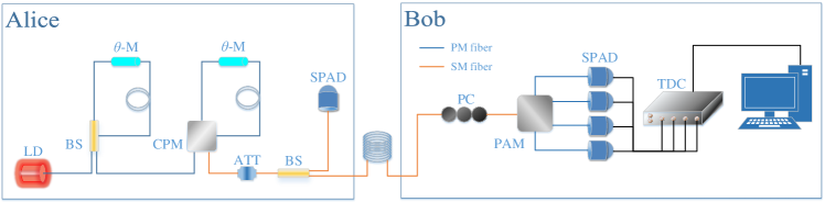
Figure 1: (Color online) Schematic diagram of BB84 QKD experimental setup. LD: 1550 nm commercial laser source; BS: beam splitter; $\theta$-M: phase modulator; CPM: customized polarization module; ATT: variable attenuator; PM fiber, polarization-maintaining fiber; SM fiber, single mode fiber; PC: polarization controller; PBS: polarized beam splitter; SPAD: single-photon avalanche detector; TDC: time-to-digital converter.

The receiver Bob possessed a PC to actively compensate for the deflection of polarization during transmission over fiber spools. The QBER of the system was used as the error signal for the active compensation. The received pulses were de-encoded using a customized polarization analysis module (PAM) integrated with a 90/10 beam splitter and two polarization-maintaining polarized beam splitters. The photons were detected using four InGaAs single-photon avalanche detectors (SPADs, WT-SPD2000, Qasky Co. LTD) with a detection efficiency of $8.8\%$, dark count rate of $10^{-6}$ per pulse, and an after pulsing probabilities of 3%. The detection events were recorded using a time-to-digital converter (TDC, quTAG100, GmbH). An optical misalignment error of approximately $1\%$ was achieved by carefully calibrating the system.

III.2 Quantifying PDL

We quantified the PDL in the source by measuring the intensity of each polarization generated by the Sagnac-PM. The measurement process was as follows. We first calibrated the expected voltages for different polarizations and determined that the voltages $\{0,~{}V_{\pi},~{}0.5V_{\pi},~{}-0.5V_{\pi}\}$ modulate the expected polarization $\{H,V,D,A\}$, where $V_{\pi}=3.8$ V. Our calibration follows a custom procedure where we scan the applied voltages of a phase modulator and record the photon detection counts D₁ and D₂. Then V_π is determined when the maximal visibility of $V=(D_{1}-D_{2})/(D_{1}+D_{2})$ is reached. Subsequently, the Sagnac-PM was directly connected to a high-precision optical power meter. Alice scanned the voltages applied to her Sagnac-PM and recorded the mean power of the optical power meter. These values were denoted by $P_{M}$. The polarization-dependent loss $L_{z(x)}$ for basis $z(x)$ was then calculated as follows:

$$L_{z(x)}=P_{H(D)}-P_{V(A)}.$$ (10)

For comparison, we also measured the PDL in recently proposed PM schemes, including an all-fiber self-compensating polarization encoder (AS-PM) Agnesi et al. (2019) and a silicon-based PM (Silicon-PM) Wei et al. (2020). The AS-PM was re-engineered with commercially available products, including a circulator and polarized beam splitter (Optizone Ltd.), phase modulator (iXblue Ltd.), and polarization controller (Thorlabs, Inc.). The Silicon-PM was manufactured by the standard fabrication service offered by IMEC foundry. The measurement process was similar to that for the Sagnac-PM. When we measured the PDL of AS-PM and Silicon-PM, the launch power of laser pulse is set to -26.557 dBm. Since the loss of Sagnac-PM is larger than previous schemes (this rises from our customized CPM), we enhanced the laser power to -20.408 dBm for making the responsivity of power meter in the linear region. All measured power and corresponding $L$ values are listed in Table 2. The table shows that all realistic PMs exhibited a PDL. In particular, the PDL was as large as 2.24 dB for a Silicon-based PM. In the table, we listed the results of the PDL in $x$ basis. These can be applied in other protocol Lim et al. (2014) where the $x$ basis is used to generate key bits. We also noticed that the PDL of Sagnac-PM is larger than that of a fiber-based polarization modulation. This is arsing from the imperfections of our in-house-designed, customized polarization module (CPM) in the Sagnac-PM. A detailed analysis can be found in Appendix B.

Table 2: Power and PDL for different polarization encoding modules. $IL$ (dB) denotes an average insertion loss. The output power $P_{M}$(dBm) represents the mean power for polarization $M$. $L_{z(x)}$ is the restored polarization loss in the $z(x)$ basis.

Module	$IL$	$P_{H}$	$P_{V}$	$P_{D}$	$P_{A}$	$L_{z}$	$L_{x}$
Sagnac-PM	23.4	$-43.488$	$-44.324$	$-43.907$	$-43.832$	$0.836$	$-0.075$
AS-PM	8.2	$-34.775$	$-34.658$	$-34.666$	$-34.853$	$-0.117$	$0.187$
Silicon-PM	5.3	$-31.08$	$-33.32$	$-32.02$	$-30.82$	$2.24$	$-1.36$

III.3 Implementation of polarization-loss-tolerant protocol

We implemented the polarization-loss-tolerant protocol over commercial fiber lengths of $25$ km, $50$ km, and $75$ km. For each distance, we optimize the implementation parameters through a numerical simulation tool, including the intensities of the signal and decoy states, the probabilities of sending them, and the post-selection probability $P_{k}$. The optimization routine was similar to that in Ref. Li et al. (2018), except we used the one-decoy-state method.

For each distance, we sent a total number of $N=10^{10}$ pulses. As indicated in Table 1, we collected the counts for different polarizations, and the details are provided in Appendix  C. By inputting the experimental counts into the one-decoy-state method presented in Sec. II, we obtained the experimental results listed in Table 3 and plotted in Fig. 2. In Table 3, the obtained QBERs for each distance are monotonically increasing because of calibration systematic error, which ranges from $0.8$ to $1.1\%$. With the polarization-loss-tolerant protocol, we achieved a secure key rate of 9.58 kbps at a distance of up to 75 km. The security of these keys considers the PDL in the PM.

Table 3: Implementation parameters and experimental results. L and Loss are the channel lengths and channel loss, respectively. $N$ is the total number of sent pulses. $\mu(\nu)$ is the intensity of signal(decoy) state, $p_{\mu}(p_{\nu})$ is the send probability of the signal(decoy) state, and $P_{\mu}(P_{\nu})$ is the post-selection probability for the signal(decoy) state. $e_{z}^{ph}$ is estimated phase error rate. $\hat{E}_{\mu}$ is obtained QBER. $l$ denotes the final key rate.

Channel		Parameter							Results
L(km)	Loss(dB)	$N$	$\mu$	$\nu$	$p_{\mu}$	$p_{\nu}$	$P_{\mu}$	$P_{\nu}$	$e_{z}^{ph}$	$\hat{E}_{\mu}$	$l$
25	4.720	$1.0020\times 10^{10}$	$0.626$	$0.157$	$0.85$	$0.15$	$0.9196$	$0.8476$	$2.90\%$	$1.04\%$	$1.43\times 10^{5}$
50	9.812	$1.0026\times 10^{10}$	$0.619$	$0.155$	$0.78$	$0.22$	$0.9189$	$0.8475$	$5.97\%$	$1.14\%$	$4.06\times 10^{4}$
75	14.970	$1.0001\times 10^{10}$	$0.611$	$0.153$	$0.67$	$0.33$	$0.9171$	$0.8470$	$8.63\%$	$1.11\%$	$9.58\times 10^{3}$

To illustrate the implications of our results, as shown in Fig. 2, we also plotted the simulation results following a standard GLLP analysis with PDL Gottesman et al. (2004). That is, we considered the PDL as small source basis-dependent flaws and applied it to the standard GLLP key rate formula, as in the study on GLLP analysis for state modulation flaws Tamaki et al. (2014); Xu et al. (2015); Tang et al. (2016). A detailed analysis can be found in Appendix D. The simulation exploited experimental parameters obtained in our setup and the PDL listed in Table 2. Fig. 2 shows that with increasing $L_{z}$, the key generation rate rapidly decreased using a standard GLLP analysis. In particular, the key generation rate dropped to zero with $L_{z}=2.24$ dB, obtained in the Silicon-PM. The maximal tolerant distance was 25 km for our setup ($L_{z}=0.836$ dB) using a previous standard GLLP analysis. In contrast, our security analysis ensures that the QKD setup is secure over 100 km, implying that for the 75-km demonstration, not even a single bit could be extracted using the previous GLLP analysis.

In our experiment, we also measure the PDL of SPADs, which is equal to zero in common sense. A value of less than 0.14 dB is obtained. However, since the PDL of SPADs results in a polarization dependency on the detection efficiency of detectors, it can be treated as a kind of detector efficiency flaws. Hence it did not influence the experimental demonstration of the polarization-loss-tolerant protocol, which focuses on the source flaws. In fact, in our previous work Wei et al. (2019), we have analyzed the impact of the polarization-dependent efficiencies on superconducting nanowire single-photon detector, and proposed some solutions to remove such a loophole.

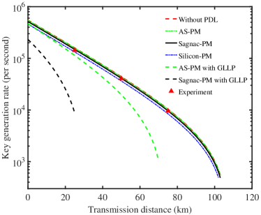
Figure 2: Secure key rate with PDL in a practical setting. The black and green and blue dotted curves represent the key rates using the one-decoy-state polarization-loss-tolerant protocol. The green and black dashed curves denote the one-decoy-state BB84 QKD with the standard GLLP analysis for PDL. The carmine triangles represent the obtained experimental results.

IV Conclusion

In summary, we demonstrated a decoy-state BB84 QKD experiment considering PDL. Following the one-decoy-state polarization-loss-tolerant protocol, we successfully generated secure key bits over different fiber links of up to 75 km. In contrast to previous experiments, which ignored the PDL in POL, the proposed study showed the feasibility of distributing secure key bits in the presence of PDL. Although we demonstrated the polarization-loss-tolerant protocol using a homemade polarization-encoding system, this method could be easily applied to other BB84-QKD systems Agnesi et al. (2020). Furthermore, it will be interesting to combine our results with other types of QKD systems, such as measurement-device-independent or twin-field QKD systems.

V Acknowledgments

We thank F. Xu and W. Li for providing the silicon chip. This study was supported by the National Natural Science Foundation of China (No. 62171144 and No. 62031024) and the Guangxi Science Foundation (Grant No. 2017GXNSFBA198231).

Appendix A Parameter estimation using one-decoy-state method

In this section, we present our one-decoy-state parameter estimation for a polarization-loss-tolerant protocol. The finite-data size was also included using the framework in Ref. Lim et al. (2014).

The total number of detections in the $\lambda$ basis is given by $n_{\lambda}=\sum_{n=0}^{\infty}s_{\lambda,n}$ ($\lambda\in{z,x}$), where $s_{\lambda,n}$ are the detection events when Alice sends an $n$-photon pulse. When PDL is present, the protocol assigns the detection counts corresponding to each polarization state $n_{\lambda,M}$ separated from the data set $n_{\lambda}$, where $M\in\{H,V,D,A\}$. In the asymptotic limit, the number of detections with a specific intensity $k\in\{\mu,\nu\}$ is given by

$$n_{z,k_{M}}^{*}=\sum_{n=0}^{\infty}p_{{k_{M}}|n}s_{z,n,M}.$$ (11)

Here, $p_{{k_{M}}|n}$ is the conditional probability, which can be expressed as $p_{{k_{M}}|n}=\frac{p_{k}}{\tau_{n,M}}\frac{e^{-k_{M}}k_{M}^{n}}{n!}$, where $\tau_{n,M}=\sum_{k\in_{\mu,\nu}}p_{k}e^{-k_{M}}k_{M}^{n}/n!$ is the probability that Alice prepares an $n$-photon pulse for polarization $M$. Here, $p_{k}$ is the probability of choosing the signal or decoy state, and $k_{M}$ represents the intensities $k$ of the state prepared in a given polarization $M$.

However, the observed data $n_{\lambda,k_{M}}$ are different from the corresponding asymptotic case when considering a finite-statistic scenario. By employing Hoeffding’s inequality Hoeffding (1963) for independent variables to bind the fluctuation, the experimental data satisfy

$$\left|n_{\lambda,k_{M}}^{*}-n_{\lambda,k_{M}}\right|\leq\delta\left(n_{\lambda},\varepsilon_{1}\right),$$ (12)

with the probability at least $1-2\varepsilon_{1}$, where $\delta\left(n_{\lambda},\varepsilon_{1}\right):=\sqrt{n_{\lambda}\log\left(1/\varepsilon_{1}\right)/2}$. The above equation allows us to obtain the upper and lower bounds of the counts $n_{\lambda,k_{M}}^{*}$ as follows:

$$n_{\lambda,k_{M}}^{*}\leqslant n_{\lambda,k_{M}}+\delta\left(n_{\lambda},\varepsilon_{1}\right)=n_{\lambda,k_{M}}^{+}$$ (13)

$$n_{\lambda,k_{M}}^{*}\geqslant n_{\lambda,k_{M}}-\delta\left(n_{\lambda},\varepsilon_{1}\right)=n_{\lambda,k_{M}}^{-}.$$

For the error detection events, we consider that the value $v_{\lambda,n}$ is the number of errors detected by Bob when Alice sends an $n$-photon pulse and $m_{\lambda}=\sum_{n=0}^{\infty}v_{\lambda,n}$ is the total number of errors in the $\lambda$ basis. In the asymptotic case corresponding to the polarization, we have

$$m_{\lambda,k_{M}}^{*}=\sum_{n=0}^{\infty}p_{{k_{M}}|n}v_{\lambda,n_{M}},\forall k\in\{\mu,\nu\}.$$ (14)

In reference to the previous case, we can determine the difference between the experimental values $m_{\lambda,k_{M}}$ and the corresponding asymptotic case $m_{\lambda,k_{M}}^{*}$, as follows:

$$\left|m_{\lambda,k_{M}}^{*}-m_{\lambda,k_{M}}\right|\leq\delta\left(m_{\lambda},\varepsilon_{2}\right)$$ (15)

with the probability of at least $1-2\varepsilon_{2}$.

Based on an estimation method proposed in Rusca et al. (2018); Lim et al. (2014), the lower bound of the vacuum counts in the $\lambda$ basis can be expressed as follows:

$$s_{\lambda,0,M}\geq s_{\lambda,0,M}^{L} :=\frac{\tau_{0,M}}{\mu_{M}-\nu_{M}}\left(\mu_{M}n_{\lambda,\nu_{M}}^{-}-\nu_{M}n_{\lambda,\mu_{M}}^{+}\right),$$ (16)

and the lower bound of the single-photon counts for polarization $M$ on the basis of $\lambda$ is given by

$$s_{\lambda,1,M}\geq s_{\lambda,1,M}^{L}: =\frac{\tau_{1,M}\mu_{M}}{\nu_{M}\left(\mu_{M}-\nu_{M}\right)}(n_{\lambda,\nu_{M}}^{-}$$ (17)

$$-\frac{\nu_{M}^{2}}{\mu_{M}^{2}}n_{\lambda,\mu_{M}}^{+}-\frac{\left(\mu_{M}^{2}-\nu_{M}^{2}\right)}{\mu_{M}^{2}}\frac{s_{\lambda,0,M}^{U}}{\tau_{0,M}}),$$

where $s_{\lambda,0,M}^{U}$ is the upper bound of the vacuum counts through the error events that can be bound by $s_{\lambda,0,M}^{U}:=2\tau_{0,M}\frac{e^{k_{M}}}{p_{k}}m_{\lambda,k_{M}}+\delta\left(n_{\lambda},\varepsilon_{1}\right)$.

Considering a specific scenario, the following formula can be used to estimate the phase error in the $z$ basis  Fung et al. (2010):

$$e_{z,1}^{ph}\leq e_{x,1}^{U}:=\frac{v_{x,1}^{U}}{s_{x,1}^{L}}+\gamma\left(\varepsilon_{sec},\frac{v_{x,1}^{U}}{s_{x,1}^{L}},s_{z,1},s_{x,1}\right)$$ (18)

where

$$\gamma(a,b,c,d)$$ (19)

$$= \sqrt{\frac{(c+d)(1-b)b}{cd\log 2}\log_{2}\left(\frac{c+d}{cd(1-b)b}\frac{21^{2}}{a^{2}}\right)}.$$

By applying the result in Lim et al. (2014), the upper bound of the number of single-photon error events in the $x$ basis for polarization $D$ is given by

$$v_{x,1,D}\leq v_{x,1,D}^{U} =\frac{\tau_{1,D}}{\mu_{D}-\nu_{D}}\left(m_{x,\mu_{D}}^{+}-m_{x,\nu_{D}}^{-}\right).$$ (20)

Similarly, the upper bound of the single-photon error events $v_{x,1,A}^{U}$ can be obtained. Combining with Eq. (17), we obtain:

$$v_{x,1}^{U} =v_{x,1,D}^{U}+v_{x,1,A}^{U},$$ (21)

$$s_{x,1}^{L} =s_{x,1,D}^{L}+s_{x,1,A}^{L}.$$

Appendix B Concise analysis of the source of Sagnac-PM PDL

The Sagnac-PM has a larger PDL than that of a fiber-based PM to conform our customized polarization module (CPM) in the Sagnac-PM, as shown in Fig. 1. We experimentally quantified the parameters including the splitter ratio $\alpha=0.872$ and the orthogonal deviation angle $\theta=0.091$ and found that these specific parameters of the CPM are larger than that of a standard commercial component. This would be the main reason for the PDL of Sagnac-PM being considerably larger than that in a fiber-based system. The detailed analysis is as follows:

When there is a deviation angle $\theta$ between orthogonal components $|H\rangle$ and $|V\rangle$, the output light from The CPM can be expressed as

$$\left|E_{1}\right\rangle=A_{1}e^{i\omega}|H\rangle,$$ (22)

and

$$\left|E_{2}\right\rangle=\alpha A_{1}e^{i\omega+\varphi}\sin\theta|H\rangle+\alpha A_{1}e^{i\omega+\varphi}\cos\theta|V\rangle,$$ (23)

where $\varphi$ is the encoded phase. Finally, the mean intensity of the light can be expressed as

$$I=\int_{0}^{2\pi}\left(\left\langle E_{1}|+\left\langle E_{2}|\right)\left(|E_{1}\right\rangle+|E_{2}\right\rangle\right)d\omega.$$ (24)

Then, the PDL of Sagnac-PM in z basis is given by

$$\mathrm{L}_{z}=10\log\frac{I(H)}{I(V)}.$$ (25)

Using the measured data, we get the theoretical value $L_{z}=0.780$ dB, which is close to the measured value of PDL of Sagnac-PM ($L_{z}=0.836$ dB).

Appendix C Detailed experimental results

Table 4 details the experimental results.

Table 4: Experimental raw counts.

Distance	$n_{x,\mu}$	$n_{x,\nu}$	$n_{z,\mu}$	$n_{z,\nu}$	$m_{x,\mu}$	$m_{x,\nu}$	$m_{z,\mu}$	$m_{z,\nu}$
$25\mathrm{~{}km}$	1302170	65577	87895811	3945456	13094	945	889766	61921
$50\mathrm{~{}km}$	377232	26907	31562239	2278091	4933	690	346762	38516
$75\mathrm{~{}km}$	87033	13457	8632164	1074008	2137	858	84805	20998
	$n_{x,\mu_{D}}$	$n_{x,\mu_{A}}$	$n_{x,\nu_{D}}$	$n_{x,\nu_{A}}$	$n_{z,\mu_{H}}$	$n_{z,\mu_{V}}$	$n_{z,\nu_{H}}$	$n_{z,\nu_{V}}$
$25\mathrm{~{}km}$	610001	692169	37460	28117	45962402	41933409	2485621	1459835
$50\mathrm{~{}km}$	192261	184971	15120	11787	16950343	14611896	1441686	836405
$75\mathrm{~{}km}$	41745	45288	7455	6002	4633555	3998609	635057	438951
	$m_{x,\mu_{D}}$	$m_{x,\mu_{A}}$	$m_{x,\nu_{D}}$	$m_{x,\nu_{A}}$	$m_{z,\mu_{H}}$	$m_{z,\mu_{V}}$	$m_{z,\nu_{H}}$	$m_{z,\nu_{V}}$
$25\mathrm{~{}km}$	8591	4503	715	230	285548	604218	19337	42584
$50\mathrm{~{}km}$	1732	3201	208	482	160264	186498	16339	22177
$75\mathrm{~{}km}$	1561	576	661	197	37191	47614	7422	13576

Appendix D Security bounds against PDL using standard GLLP analysis

In this section, we discuss how we can bound information leakage caused by PDL using standard GLLP security analysis. We consider the PDL in state-preparation devices as a type of source flaw. Hence, the key rate formula is similar to that in Eq. (1) in the main text, except that the phase error rate needs to include the correction due to source flaws. Based on the GLLP analysis, PDL can be quantified using the so-called quantum coin $\Delta$, which is given by

$$\Delta=\frac{1-F\left(\rho_{z},\rho_{x}\right)}{2},$$ (26)

where $F\left(\rho_{z},\rho_{x}\right)$ is the fidelity of the density matrices for the $z$ and $x$ bases. The balance of a quantum coin quantifies the basis-dependent flaws of Alice’s single-photon components or the ability to discriminate the bases that Eve possesses. For simplicity, we introduce the idea of an entanglement-based scenario to provide an imperfect parameter value, which is equivalent to a prepare-and-measure protocol. Here, Alice first generates an entangled state as follows:

$$\left|\Upsilon_{z}\right\rangle_{AB}=\sqrt{\frac{1}{l_{z}+1}}\left|0_{z}\right\rangle_{A}\otimes\left|0_{z}\right\rangle_{B}+\sqrt{\frac{l_{z}}{l_{z}+1}}\left|1_{z}\right\rangle_{A}\otimes\left|1_{z}\right\rangle_{B}$$ (27)

and sends System B to Bob. Here, the coefficient $l_{z}$ depends on the polarization-dependent loss $L_{z}$, which can be expressed by $l_{z}=10^{-L_{z}/10}$. In the virtual protocol, Alice can measure system A after Bob detects and Eve makes a disturbance. In Eq. (27), we consider the PDL, from which the coefficient of the state is related to $L_{z}$, satisfying normalization. Similarly, for each $x$ basis emission, Alice prepares the entangled states as follows:

$$\left|\Upsilon_{x}\right\rangle_{AB}=\sqrt{\frac{1}{l_{x}+1}}\left|0_{x}\right\rangle_{A}\otimes\left|0_{x}\right\rangle_{B}+\sqrt{\frac{l_{x}}{l_{x}+1}}\left|1_{x}\right\rangle_{A}\otimes\left|1_{x}\right\rangle_{B}$$ (28)

and sends System B to Bob. The coefficient $l_{x}$ depends on the PDL on the $x$ basis. Evidently, the states $\left|\Upsilon_{z}\right\rangle_{AB}$ and $\left|\Upsilon_{x}\right\rangle_{AB}$ are no longer equal because of the imperfect state preparation. Furthermore, by introducing a quantum coin, Alice prepares an entangled state following  Koashi (2009)

$$|\Gamma\rangle_{CAB} =\frac{1}{2}\left[|0_{x}\rangle_{C}\left(\left|\Upsilon_{z}\right\rangle_{AB}\right.\right.$$ (29)

$$+\left|\Upsilon_{x}\right\rangle_{AB})+\left|1_{x}\right\rangle_{C}\left(\left|\Upsilon_{z}\right\rangle_{AB}-\left|\Upsilon_{x}\right\rangle_{AB}\right)],$$

where system C is ”a quantum coin,” determining that each signal is encoded on a $z$ or $x$ basis. If the quantum-coin system collapses into the state $\left|1_{x}\right\rangle_{C}$, we can obtain the probability quantifying how well the basis dependence of Alice’s and Bob’s single-photon pairs, so that we have

$$\Delta=\operatorname{Prob}\left(X_{C}=-1\right) =\left.\left.\right|_{C}\left\langle 1_{x}\mid\Gamma\right\rangle_{CAB}\right|^{2}$$ (30)

$$=\frac{1}{2}(1-\frac{(1+\sqrt{l_{z}})(1+\sqrt{l_{x}})}{\sqrt{(l_{z}+1)(l_{x}+1)}}).$$

In our QKD system, with $L_{z(x)}=0.836(-0.075)$, we have $\Delta=5.82\times 10^{-4}$. Thus, based on Eq. (26), the fidelity $F\left(\rho_{z},\rho_{x}\right)=1-1.16\times 10^{-3}$. In the GLLP analysis, the basis-dependent flaws of Alice’s signals associated with single-photon events can be enhanced in principle by Eve by exploiting the channel loss; thus, $\Delta$ is replaced by $\Delta^{\prime}$ as follows:

$$\Delta^{\prime}=\frac{\Delta}{Y_{1}},$$ (31)

where $Y_{1}$ is the yield of the $1$-photon pulses. The revised phase error rate can be expressed as

$$\bar{e}_{z}^{ph}\leqslant e_{x,1}^{U}+4\Delta^{\prime}+4\sqrt{\Delta^{\prime}e_{x,1}^{U}}+\epsilon_{ph}.$$ (32)

By substituting Eq. (32) into Eq. (1), we obtain the final key rate using the standard GLLP approach while considering the PDL. The simulation results are presented in Fig. 2.

References

- Lo and Chau (1999) H.-K. Lo and H. F. Chau, Science 283, 2050 (1999).
- Choi et al. (2016) Y. Choi, O. Kwon, M. Woo, K. Oh, S.-W. Han, Y.-S. Kim, and S. Moon, Phys. Rev. A 93, 032319 (2016).
- Cañas et al. (2017) G. Cañas, N. Vera, J. Cariñe, P. González, J. Cardenas, P. W. R. Connolly, A. Przysiezna, E. S. Gómez, M. Figueroa, G. Vallone, P. Villoresi, T. F. da Silva, G. B. Xavier, and G. Lima, Phys. Rev. A 96, 022317 (2017).
- Boaron et al. (2018) A. Boaron, G. Boso, D. Rusca, C. Vulliez, C. Autebert, M. Caloz, M. Perrenoud, G. Gras, F. Bussières, M.-J. Li, D. Nolan, A. Martin, and H. Zbinden, Phys. Rev. Lett. 121, 190502 (2018).
- Liu et al. (2010) Y. Liu, T.-Y. Chen, J. Wang, W.-Q. Cai, X. Wan, L.-K. Chen, J.-H. Wang, S.-B. Liu, H. Liang, L. Yang, C.-Z. Peng, K. Chen, Z.-B. Chen, and J.-W. Pan, Opt. Express 18, 8587 (2010).
- Wang et al. (2012) S. Wang, W. Chen, J.-F. Guo, Z.-Q. Yin, H.-W. Li, Z. Zhou, G.-C. Guo, and Z.-F. Han, Opt. Lett. 37, 1008 (2012).
- Ma et al. (2021) D. Ma, X. Liu, C. Huang, H. Chen, H. Lin, and K. Wei, Opt. Lett. 46, 2152 (2021).
- Zhou et al. (2021) X.-Y. Zhou, H.-J. Ding, M.-S. Sun, S.-H. Zhang, J.-Y. Liu, C.-H. Zhang, J. Li, and Q. Wang, Phys. Rev. Appl. 15, 064016 (2021).
- Bunandar et al. (2018) D. Bunandar, A. Lentine, C. Lee, H. Cai, C. M. Long, N. Boynton, N. Martinez, C. DeRose, C. Chen, M. Grein, D. Trotter, A. Starbuck, A. Pomerene, S. Hamilton, F. N. ? Wong, R. Camacho, P. Davids, J. Urayama, and D. Englund, Phys. Rev. X 8, 021009 (2018).
- Liao et al. (2017) S.-K. Liao, W.-Q. Cai, W.-Y. Liu, L. Zhang, Y. Li, J.-G. Ren, J. Yin, Q. Shen, Y. Cao, Z.-P. Li, et al., Nature 549, 43 (2017).
- Chen et al. (2020) H. Chen, J. Wang, B. Tang, Z. Li, B. Liu, and S. Sun, Opt. Lett. 45, 3022 (2020).
- Avesani et al. (2021) M. Avesani, L. Calderaro, M. Schiavon, A. Stanco, C. Agnesi, A. Santamato, M. Zahidy, A. Scriminich, G. Foletto, G. Contestabile, M. Chiesa, D. Rotta, M. Artiglia, A. Montanaro, M. Romagnoli, V. Sorianello, F. Vedovato, G. Vallone, and P. Villoresi, Npj Quantum Inf. 7, 93 (2021).
- Hu et al. (2019) C.-Q. Hu, Z.-Q. Yan, J. Gao, Z.-Q. Jiao, Z.-M. Li, W.-G. Shen, Y. Chen, R.-J. Ren, L.-F. Qiao, A.-L. Yang, H. Tang, and X.-M. Jin, Photon. Res. 7, A40 (2019).
- Chen et al. (2010) T.-Y. Chen, J. Wang, H. Liang, W.-Y. Liu, Y. Liu, X. Jiang, Y. Wang, X. Wan, W.-Q. Cai, L. Ju, L.-K. Chen, L.-J. Wang, Y. Gao, K. Chen, C.-Z. Peng, Z.-B. Chen, and J.-W. Pan, Opt. Express 18, 27217 (2010).
- Sasaki et al. (2011) M. Sasaki, M. Fujiwara, H. Ishizuka, W. Klaus, K. Wakui, M. Takeoka, S. Miki, T. Yamashita, Z. Wang, and A. Tanaka, Opt. Express 19, 10387 (2011).
- Wang et al. (2014) S. Wang, W. Chen, Z.-Q. Yin, H.-W. Li, D.-Y. He, Y.-H. Li, Z. Zhou, X.-T. Song, F.-Y. Li, D. Wang, H. Chen, Y.-G. Han, J.-Z. Huang, J.-F. Guo, P.-L. Hao, M. Li, C.-M. Zhang, D. Liu, W.-Y. Liang, C.-H. Miao, P. Wu, G.-C. Guo, and Z.-F. Han, Opt. Express 22, 21739 (2014).
- Dynes et al. (2019) J. F. Dynes, A. Wonfor, W. W. S. Tam, A. W. Sharpe, R. Takahashi, M. Lucamarini, A. Plews, Z. L. Yuan, A. R. Dixon, J. Cho, Y. Tanizawa, J. P. Elbers, H. Greier, I. H. White, R. V. Penty, and A. J. Shields, Npj Quantum Inf. 5, 101 (2019).
- Yang et al. (2021) Y.-H. Yang, P.-Y. Li, S.-Z. Ma, X.-C. Qian, K.-Y. Zhang, L.-J. Wang, W.-L. Zhang, F. Zhou, S.-B. Tang, J.-Y. Wang, Y. Yu, Q. Zhang, and J.-W. Pan, Opt. Express 29, 25859 (2021).
- Chen et al. (2021a) Y.-A. Chen, Q. Zhang, T.-Y. Chen, W.-Q. Cai, S.-K. Liao, J. Zhang, K. Chen, J. Yin, J.-G. Ren, Z. Chen, S.-L. Han, Q. Yu, K. Liang, F. Zhou, X. Yuan, M.-S. Zhao, T.-Y. Wang, X. Jiang, L. Zhang, W.-Y. Liu, Y. Li, Q. Shen, Y. Cao, C.-Y. Lu, R. Shu, J.-Y. Wang, L. Li, N.-L. Liu, F. Xu, X.-B. Wang, C.-Z. Peng, and J.-W. Pan, Nature 589, 214 (2021a).
- Chen et al. (2021b) J.-P. Chen, C. Zhang, Y. Liu, C. Jiang, W.-J. Zhang, Z.-Y. Han, S.-Z. Ma, X.-L. Hu, Y.-H. Li, H. Liu, F. Zhou, H.-F. Jiang, T.-Y. Chen, H. Li, L.-X. You, Z. Wang, X.-B. Wang, Q. Zhang, and J.-W. Pan, Nature Photon. 15, 570 (2021b).
- Pittaluga et al. (2021) M. Pittaluga, M. Minder, M. Lucamarini, M. Sanzaro, R. I. Woodward, M.-J. Li, Z. Yuan, and A. J. Shields, Nature Photon. 15, 530 (2021).
- Lo et al. (2012) H.-K. Lo, M. Curty, and B. Qi, Phys. Rev. Lett. 108, 130503 (2012).
- Lucamarini et al. (2018) M. Lucamarini, Z. L. Yuan, J. F. Dynes, and A. J. Shields, Nature 557, 400 (2018).
- Ma et al. (2018) X. Ma, P. Zeng, and H. Zhou, Phys. Rev. X 8, 031043 (2018).
- Wang et al. (2018) X.-B. Wang, Z.-W. Yu, and X.-L. Hu, Phys. Rev. A 98, 062323 (2018).
- Wang et al. (2019) S. Wang, D.-Y. He, Z.-Q. Yin, F.-Y. Lu, C.-H. Cui, W. Chen, Z. Zhou, G.-C. Guo, and Z.-F. Han, Phys. Rev. X 9, 021046 (2019).
- Gottesman et al. (2004) D. Gottesman, H.-K. Lo, N. Lütkenhaus, and J. Preskill, Quantum Inf. Comput. 4, 325 (2004).
- Qian et al. (2018) Y.-J. Qian, D.-Y. He, S. Wang, W. Chen, Z.-Q. Yin, G.-C. Guo, and Z.-F. Han, Phys. Rev. Appl. 10, 064062 (2018).
- Yoshino et al. (2018) K.-i. Yoshino, M. Fujiwara, K. Nakata, T. Sumiya, T. Sasaki, M. Takeoka, M. Sasaki, A. Tajima, M. Koashi, and A. Tomita, Npj Quantum Inf. 4, 8 (2018).
- Wei et al. (2019) K. Wei, W. Zhang, Y.-L. Tang, L. You, and F. Xu, Phys. Rev. A 100, 022325 (2019).
- Huang et al. (2020) A. Huang, R. Li, V. Egorov, S. Tchouragoulov, K. Kumar, and V. Makarov, Phys. Rev. Appl. 13, 034017 (2020).
- Pang et al. (2020) X.-L. Pang, A.-L. Yang, C.-N. Zhang, J.-P. Dou, H. Li, J. Gao, and X.-M. Jin, Phys. Rev. Appl. 13, 034008 (2020).
- Xu et al. (2020) F. Xu, X. Ma, Q. Zhang, H.-K. Lo, and J.-W. Pan, Rev. Mod. Phys. 92, 025002 (2020).
- Tang et al. (2013) Y.-L. Tang, H.-L. Yin, X. Ma, C.-H. F. Fung, Y. Liu, H.-L. Yong, T.-Y. Chen, C.-Z. Peng, Z.-B. Chen, and J.-W. Pan, Phys. Rev. A 88, 022308 (2013).
- Sibson et al. (2017) P. Sibson, J. E. Kennard, S. Stanisic, C. Erven, J. L. O’Brien, and M. G. Thompson, Optica 4, 172 (2017).
- Agnesi et al. (2019) C. Agnesi, M. Avesani, A. Stanco, P. Villoresi, and G. Vallone, Opt. Lett. 44, 2398 (2019).
- Li et al. (2019) Y. Li, Y.-H. Li, H.-B. Xie, Z.-P. Li, X. Jiang, W.-Q. Cai, J. Wang, J. Yin, L. Shengkai, and C.-Z. Peng, Opt. Lett. 44, 5262 (2019).
- Wei et al. (2020) K. Wei, W. Li, H. Tan, Y. Li, H. Min, W.-J. Zhang, H. Li, L. You, Z. Wang, X. Jiang, T.-Y. Chen, S.-K. Liao, C.-Z. Peng, F. Xu, and J.-W. Pan, Phys. Rev. X 10, 031030 (2020).
- Li et al. (2018) C. Li, M. Curty, F. Xu, O. Bedroya, and H.-K. Lo, Phys. Rev. A 98, 042324 (2018).
- Rusca et al. (2018) D. Rusca, A. Boaron, F. Grünenfelder, A. Martin, and H. Zbinden, Appl. Phys. Lett. 112, 171104 (2018).
- Wang (2005) X.-B. Wang, Phys. Rev. Lett. 94, 230503 (2005).
- Lo et al. (2005) H.-K. Lo, X. Ma, and K. Chen, Phys. Rev. Lett. 94 (2005), 10.1103/PhysRevLett.94.230504.
- Lim et al. (2014) C. C. W. Lim, M. Curty, N. Walenta, F. Xu, and H. Zbinden, Phys. Rev. A 89, 022307 (2014).
- Ma et al. (2016) C. Ma, W. D. Sacher, Z. Tang, J. C. Mikkelsen, Y. Yang, F. Xu, T. Thiessen, H.-K. Lo, and J. K. S. Poon, Optica 3, 1274 (2016).
- Tamaki et al. (2014) K. Tamaki, M. Curty, G. Kato, H.-K. Lo, and K. Azuma, Phys. Rev. A 90, 052314 (2014).
- Xu et al. (2015) F. Xu, K. Wei, S. Sajeed, S. Kaiser, S. Sun, Z. Tang, L. Qian, V. Makarov, and H.-K. Lo, Phys. Rev. A 92, 032305 (2015).
- Tang et al. (2016) Z. Tang, K. Wei, O. Bedroya, L. Qian, and H.-K. Lo, Phys. Rev. A 93, 042308 (2016).
- Agnesi et al. (2020) C. Agnesi, M. Avesani, L. Calderaro, A. Stanco, G. Foletto, M. Zahidy, A. Scriminich, F. Vedovato, G. Vallone, and P. Villoresi, Optica 7, 284 (2020).
- Hoeffding (1963) W. Hoeffding, J. Am. Stat. Assoc. 58, 13 (1963).
- Fung et al. (2010) C.-H. F. Fung, X. Ma, and H. F. Chau, Phys. Rev. A 81, 012318 (2010).
- Koashi (2009) M. Koashi, New J. Phys. 11, 045018 (2009).