Novel solitary and periodic waves in quadratic-cubic non-centrosymmetric waveguides

Abstract

We present a wide class of novel solitary and periodic waves in a non-centrosymmetric waveguide exhibiting second- and third-order nonlinearities. We show the existence of bright, gray, and W-shaped solitary waves as well as periodic waves for extended nonlinear Schrödinger equation with quadratic and cubic nonlinearities. We also obtained the exact analytical algebraic-type solitary waves of the governing equation, including bright and W-shaped waves. The results illustrate the propagation of potentially rich set of nonlinear structures through the optical waveguiding media. Such privileged waveforms characteristically exist due to a balance among diffraction, quadratic and cubic nonlinearities.

I Introduction

Interest in nonlinear localized waves also called solitons has grown considerably in recent times due to their appearance in various physical systems. The occurrence of such structures range from fluid dynamics Kodama10 , Bose-Einstein condensates Burger -Strecker , fiber-optic communications and photonics in general L ; Y , to nuclear physics Arriola , and plasmas physics Infeld ; Shukla . The research results have shown that there exist two distinct functional forms of localized waves, hyperbolic and algebraic forms, which play the same role in the wave dynamics. It is worthwhile to mention here that algebraic-type solitary waves are localized more weakly compared with the conventional (hyperbolic) solitons Hayata .

Theoretically, the study of propagation properties of localized waves in a Kerr dielectric guide involves solving the nonlinear Schrödinger (NLS) equation that includes the group velocity dispersion and self-phase modulation Kodama . Such underlying model has also been applied to the description of matter waves in Bose-Einstein condensates Beitia . In the latter setting, the equation is usually called the Gross- Pitaevskii equation (GPE) Pitaevskii . We mention in passing that the NLS model is also relevant for electromagnetic pulse propagation in negative index materials Scalora .

Recent advances in the study of optical materials have demonstrated that the application of the NLS model for a more realistic description of wave dynamics in many practical materials imposes the inclusion of additional nonlinear and dispersive terms in the underlying equation Avelar -Nikola . In this context, several generalizations of the NLS equation with different forms of nonlinearities have been developed to study the wave evolution in diverse physical systems, including cubic-quintic Avelar , cubic-quintic-septimal R ; TH , polynomial Nikola , and saturable Vasantha nonlinearity. The quadratic-cubic NLS equation is a newly extension of the NLS equation which has gathered significant attention in recent years. Such equation may be used as an approximate form of the GPE for quasi-one-dimensional Bose-Einstein condensate with contact repulsion and dipole-dipole attraction Fujioka . This model can be also applied for the description of light beam propagation in a non-centrosymmetric waveguide exhibiting second- and third-order nonlinearity Pal . Due to its physical importance, this nonlinear wave evolution equation has been analyzed from different points of view. For instance, Cardoso et al. have obtained the localized solutions for inhomogeneous quadratic-cubic NLS equation and studied their stability with respect to small random perturbations Cardoso . Triki et al. have analyzed this equation with space and time modulated nonlinearities in presence of external potentials in the context of Bose-Einstein condensates TH0 . In TH1 , the soliton solutions and the conservation laws of the equation were reported. In Pal , the chirped self-similar wave solutions of the equation were constructed by employing the similarity transformation method. Some soliton solutions of the equation have been also obtained by means of the extended trial equation method in TH2 .

Looking for more novel solutions to quadratic-cubic NLS model is an important direction in the studies of nonlinear matter and optical wave propagations. In particular, obtaining new solutions in analytic form will be a remarkable contribution to well understand physical phenomena in various dynamical systems where the quadratic-cubic NLS equation can provide a realistic description of the waves. In this paper, we present new types of exact analytical localized and periodic wave solutions for the quadratic-cubic NLS equation.

The paper is organized as follows. In Sec. II, we present the quadratic-cubic NLS model describing the propagation of light beams in non-centrosymmetric waveguides, and we give a detailed study of families of novel solitary and periodic wave solutions of the model. We also examine here the existence condition for algebraic solitary waves of the underlying equation. Finally, we present some conclusions in Sec. III.

II Model and novel solitary and periodic wave solutions

The propagation of light beams in quadratic-cubic non-centrosymmetric waveguides is modeled by the following quadratic-cubic NLS equation TH1 ; Pal ; TH2 ,

$$i\frac{\partial E}{\partial z}-\frac{\alpha}{2}\frac{\partial^{2}E}{\partial x^{2}}+\sigma|E|E+\nu|E|^{2}E=0,$$ (1)

where $z$ is the longitudinal variable representing propagation distance, $x$ is transverse variable, and $E(z,x)$ is the complex envelope of the electrical field. The parameters $\alpha,$ $\sigma$ and $\nu$ represent the diffraction, quadratic and cubic nonlinearity coefficients, respectively.

To find exact solutions of Eq. (1), we consider an ansatz solution of the form VK ,

$$E(z,x)=u(\xi)\exp[i\left(\kappa z-\Omega x+\theta\right)],$$ (2)

where $u$ is a differentiable real function depending on the variable $\xi=x-qz$, with $q=v^{-1}$ being the inverse velocity of the wave packet. Also, $\kappa$ and $\Omega$ are the respective real parameters describing the wave number and frequency shift, while $\theta$ represents the phase of the pulse at $z=0$.

Inserting Eq. (2) into Eq. (1) and separating real and imaginary parts, we obtain,

$$q=\alpha\Omega,$$ (3)

from the imaginary part, indicating that the inverse velocity $q$ is controlled by the parameters $\alpha$ and $\Omega$. The real part yields the equation,

$$-\kappa u-\frac{\alpha}{2}\frac{d^{2}u}{d\xi^{2}}+\frac{\alpha\Omega^{2}}{2}u+\sigma|u|u+\nu u^{3}=0,$$ (4)

The latter can expressed in the form

$$\frac{d^{2}u}{d\xi^{2}}+au^{3}+b|u|u+cu=0,$$ (5)

where the parameters $a$, $b$ and $c$ are given by

$$a=-\frac{2\nu}{\alpha},\qquad b=-\frac{2\sigma}{\alpha},\qquad c=\frac{2\kappa-\alpha\Omega^{2}}{\alpha}.$$ (6)

Nonlinear differential equation (5) with coexisting quadratic $|u|u$ and cubic $u^{3}$ describes the evolution dynamics of the field amplitude as it propagates through the non-centrosymmetric waveguide. Nonlinear waveforms propagating inside the waveguiding media can be readily obtained by solving this nonlinear differential equation. We emphasis that the term $b|u|u$ in Eq. (5) has two different forms for positive and negative values of the function $u(\xi)$:

$$b|u|u=bu^{2}~{}~{}~{}(for~{}u(\xi)\geq 0),\qquad b|u|u=-bu^{2}~{}~{}~{}(for~{}u(\xi)\leq 0).$$ (7)

This feature is crucial for obtained exact solutions presented below. In the following, we present novel exact solitary and periodic wave solutions for Eq. (1) obtained by substitution of closed form solutions of the nonlinear differential equation (5) into the ansatz solution (2). To our knowledge, the gray solitary wave (16), W-shaped solitary waves (17) and (18), periodic wave solutions (23) and (29) presented below are firstly reported in this work. Such privileged exact solutions are formed in the optical waveguiding media due to a balance among diffraction, quadratic and cubic nonlinearities.

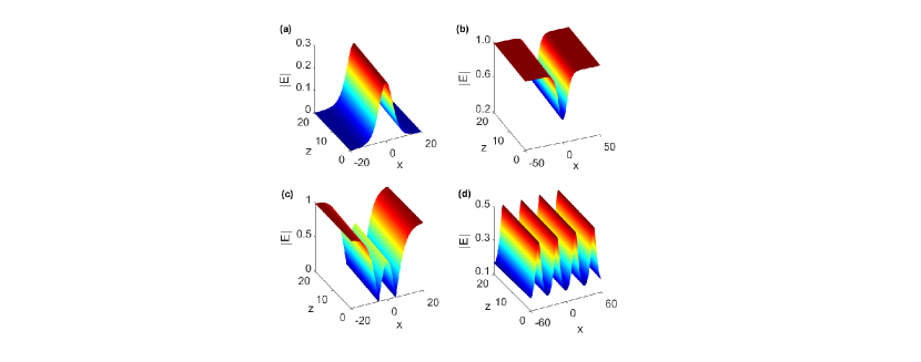
Figure 1: Evolution of nonlinear wave solutions (a) bright solitary wave (11) with parameters $\alpha=1,$ $\sigma=-0.5,$ $\nu=0.25,$ $q=0.1,$ $z_{0}=0,$ $\Omega=1,$ and $\kappa=0.42$ (b) gray solitary wave (16) with parameters $\alpha=2,$ $\sigma=-0.5,$ $\nu=0.3,$ $q=0.1,$ $z_{0}=0,$ $\Omega=1,$ and $\kappa=0.8$ (c) W-shaped solitary wave (17) with parameters $\alpha=2,$ $\sigma=\frac{1}{15},$ $\nu=\frac{1}{45},$ $q=0.1,$ $z_{0}=0,$ $\Omega=\frac{1}{3},$ and $\kappa=0.2$ (d) periodic wave (23) with parameters $\alpha=1,$ $\sigma=0.25,$ $\nu=-0.5,$ $q=0.1,$ $z_{0}=0,$ $\kappa=\frac{25}{48}$ and $\Omega=1$.

1. Bright solitary waves

The nonlinear differential equation (5) supports the exact solitary wave solution as

$$u(\xi)=\frac{A}{1+D\cosh(w(\xi-\xi_{0}))}.$$ (8)

There are two different cases for parameters in Eq. (8). In the first case [$u(\xi)\geq 0$], the real parameters $w$, $A$ and $D$ are given by

$$w=\sqrt{-c},\qquad A=-\frac{3c}{b},$$ (9)

$$D=\sqrt{1-\frac{9ac}{2b^{2}}},$$ (10)

where $c<0$ and $9ac/2b^{2}<1$. In the second case [$u(\xi)\leq 0$] the parameters $w$ and $D$ have the same form, however the parameter $A$ is given as $A=3c/b$. This is connected with relations in Eq. (7) which yield in this second case the replacement of parameter $b$ to $-b$. The exact solution of Eq. (1) for these two cases has the form,

$$E(z,x)=\frac{A}{1+D\cosh(w(x-q(z-z_{0})))}\exp[i\left(\kappa z-\Omega x+\theta\right)].$$ (11)

Figure 1(a) presents an example of propagation of the solitary wave solution (11) for the parameter values $\alpha=1,$ $\sigma=-0.5,$ $\nu=0.25,$ $q=0.1,$ $z_{0}=0,$ $\Omega=1,$ and $\kappa=0.42$. It is interesting to note that the structure is a bright pulse on a zero background.

2. Gray and dark solitary waves

We have obtained the gray solitary wave solution for Eq. (5) as follows:

$$u(\xi)=\lambda-\frac{B}{1+D\cosh(w(\xi-\xi_{0}))}.$$ (12)

Note that Eq. (12) describes the gray solitary waves for two different cases: (1) $u(\xi)>0$, and (2) $u(\xi)<0$. In the first case [$u(\xi)>0$] we have the conditions as $\lambda>0$ and $\lambda-B/(1+D)>0$. In this case the parameter $\lambda$ is given by equation $a\lambda^{2}+b\lambda+c=0$ which yields

$$\lambda=\frac{1}{2a}\left(-b\pm\sqrt{b^{2}-4ac}\right).$$ (13)

The parameters $w$, $B$ and $D$ are given by

$$w=\sqrt{2c+b\lambda},\qquad B=-\frac{3(2c+b\lambda)}{b+3a\lambda},$$ (14)

$$D=\left[1+\frac{9a(2c+b\lambda)}{2(b+3a\lambda)^{2}}\right]^{1/2}.$$ (15)

In the second case [$u(\xi)<0$] we have the conditions as $\lambda<0$ and $\lambda-B/(1+D)<0$. The relations in (7) yield in this case the replacement of parameter $b$ to $-b$ in Eqs. (13-15). The exact gray solitary wave solutions of Eq. (1) for two cases [with $u(\xi)>0$ and $u(\xi)<0$] are given by

$$E(z,x)=\left(\lambda-\frac{B}{1+D\cosh(w(x-q(z-z_{0})))}\right)\exp[i\left(\kappa z-\Omega x+\theta\right)].$$ (16)

We emphasis that Eq. (13) defines two different values for parameters $\lambda$. Hence, the above solitary waves are determined for each value of $\lambda$.

In Fig. 1(b), we have plotted an example of propagation of the gray solitary wave solution (16) for the parameter values $\alpha=2,$ $\sigma=-0.5,$ $\nu=0.3,$ $q=0.1,$ $z_{0}=0,$ $\Omega=1,$ and $\kappa=0.8$. To find the value of the parameter $\lambda$, we have considered the case of lower sign in Eq. (13). We note that the dark solitary wave solutions are the particular cases of these gray solitary wave solutions when the constraint $\lambda=B/(1+D)$ is satisfied.

3. W-shaped solitary waves

We have also obtained two W-shaped solitary wave solutions for Eq. (1). The first case takes place when the conditions $\lambda>0$ and $\lambda-B/(1+D)<0$ are satisfied. The W-shaped solitary wave solution in this case has the form,

$$E(z,x)=\left|\lambda-\frac{B}{1+D\cosh(w(x-q(z-z_{0})))}\right|\exp[i\left(\kappa z-\Omega x+\theta\right)],$$ (17)

where the parameters $\lambda$, $w$, $B$ and $D$ are given by Eqs. (13-15).

The second case takes place when the following conditions $\lambda<0$ and $\lambda-B/(1+D)>0$ are satisfied. The W-shaped solitary wave solution in this case has the form,

$$E(z,x)=-\left|\lambda-\frac{B}{1+D\cosh(w(x-q(z-z_{0})))}\right|\exp[i\left(\kappa z-\Omega x+\theta\right)],$$ (18)

where the parameters $\lambda$, $w$, $B$ and $D$ are given by Eqs. (13-15) with the replacement of parameter $b$ to $-b$.

Figure 1(c) displays the propagation of the solitary wave solution (17) for the parameter values $\alpha=2,$ $\sigma=\frac{1}{15},$ $\nu=\frac{1}{45},$ $q=0.1,$ $z_{0}=0,$ $\Omega=\frac{1}{3},$ and $\kappa=0.2$. To find the value of the parameter $\lambda$, we have considered the case of lower sign in Eq. (13). One can see from this figure that the structure takes the shape of W, which can be formed in the waveguide medium due to a balance among the diffraction and quadratic-cubic nonlinearities.

4. Periodic waves

We have also obtained an exact periodic wave solution for Eq. (5) as

$$u(\xi)=\frac{A}{B+\cos(w(\xi-\xi_{0}))},$$ (19)

where the real parameters $w$ and $B$ are

$$w=\sqrt{c},\qquad B=\frac{\pm 1}{\sqrt{1-Q}},\qquad Q=\frac{9ac}{2b^{2}},$$ (20)

with $c>0$ and $Q<1$. The real parameter $A$ is given by

$$A=\mp\frac{3c}{b\sqrt{1-Q}}.$$ (21)

The periodic wave in Eq. (19) is a bounded solution for the condition $|B|>1$, which yields $Q>0$. Hence, we have the following conditions for the bounded periodic solution given in Eq. (19):

$$c>0,\qquad 0<\frac{9ac}{2b^{2}}<1.$$ (22)

The exact periodic bounded wave solution of Eq. (1) has the form,

$$E(z,x)=\frac{A}{B+\cos(w(x-q(z-z_{0})))}\exp[i\left(\kappa z-\Omega x+\theta\right)].$$ (23)

An example of propagation of the nonlinear wave solution (23) is shown in Fig. 1(d) for the parameter values $\alpha=1,$ $\sigma=0.25,$ $\nu=-0.5,$ $q=0.1,$ $z_{0}=0,$ $\kappa=\frac{25}{48}$ and $\Omega=1$. It is interesting to see that this structure presents an oscillating behaviour superimposed at a nonzero background.

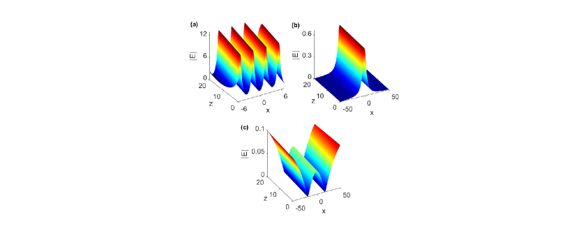
Figure 2: Evolution of nonlinear wave solutions (a) modified periodic wave (29) with parameters $\alpha=-1,$ $\sigma=0.5,$ $\nu=0.5,$ $q=0.1,$ $z_{0}=0,$ $\Omega=1,$ and $\kappa=0.5$ (b) bright algebraic solitary wave (34) with parameters $\alpha=1,$ $\sigma=0.25,$ $\nu=-0.5,$ $z_{0}=0,$ $\Omega=2,$ $q=0.1$, and $\kappa=2$ (c) W-shaped algebraic solitary wave (38) with parameters $\alpha=-1,$ $\sigma=0.03,$ $\nu=0.1,$ $\kappa=0.00045,$ $q=0.2,$ $\Omega=0.06,$ and $z_{0}=0$.

5. Modified periodic waves

We have also obtained modified periodic wave solution for Eq. (5) as follows:

$$u(\xi)=\left|\lambda-\frac{A}{B+\cos(w(\xi-\xi_{0}))}\right|,$$ (24)

where $\lambda\neq 0$. In this case the parameter $\lambda$ is given by equation $a\lambda^{2}+b\lambda+c=0$. The real parameters $\lambda$, $w$ and $B$ are

$$\lambda=\frac{1}{2a}\left(-b\pm\sqrt{b^{2}-4ac}\right),\qquad w=\sqrt{-2c-b\lambda},$$ (25)

$$B=\frac{\pm 1}{\sqrt{1+R}},\qquad R=\frac{9a(2c+b\lambda)}{2(b+3a\lambda)^{2}},$$ (26)

where $b^{2}>4ac$, $2c+b\lambda<0$ and $R>-1$. Also, the parameter $A$ is given by

$$A=\mp\frac{3(2c+b\lambda)}{(b+3a\lambda)\sqrt{1+R}}.$$ (27)

Another solution has the form,

$$u(\xi)=-\left|\lambda-\frac{A}{B+\cos(w(\xi-\xi_{0}))}\right|,$$ (28)

where $\lambda\neq 0$. The parameters in this solution follow from Eqs. (25-27) with the replacement of parameter $b$ to $-b$. Thus the appropriate modified periodic bounded solutions of Eq. (1) are

$$E(z,x)=\pm\left|\lambda-\frac{A}{B+\cos(w(x-q(z-z_{0})))}\right|\exp[i\left(\kappa z-\Omega x+\theta\right)].$$ (29)

In Fig. 2(a), we have presented an example of propagation of the nonlinear wave solution (29) for the parameter values $\alpha=-1,$ $\sigma=0.5,$ $\nu=0.5,$ $q=0.1,$ $z_{0}=0,$ $\Omega=1,$ and $\kappa=0.5$. To get the value of the parameter $\lambda$, we have considered the case of upper sign in Eq. (25). It is clear from the figure that the profile of the wave presents the periodic property as it propagates inside the waveguide.

6. Bright algebraic solitary waves

The nonlinear differential equation (5) supports the exact algebraic-type solitary wave solution:

$$u(\xi)=\frac{p}{1+\mu(\xi-\xi_{0})^{2}}.$$ (30)

There are two different cases for parameters in Eq. (30). In the first case [$u(\xi)\geq 0$] the real parameters $p$ and $\mu$ are defined by the expressions,

$$p=-\frac{4b}{3a},\qquad\mu=\frac{2b^{2}}{9a},$$ (31)

and $c=0$ in Eq. (6). Thus the wave number $\kappa$ of this optical wave solution is given by

$$\kappa=\frac{1}{2}\alpha\Omega^{2}.$$ (32)

In this case [$u(\xi)\geq 0$] we have the conditions $p>0$ and $\mu>0$ which yield $a>0$ and $b<0$.

In the second case [$u(\xi)\leq 0$] the real parameters $p$ and $\mu$ are defined by the expressions,

$$p=\frac{4b}{3a},\qquad\mu=\frac{2b^{2}}{9a},$$ (33)

and $c=0$ in Eq. (6). We replaced here $b$ to $-b$ which follows from relations in Eq. (7). Thus in this second case we have the conditions $p<0$ and $\mu>0$ which yield $a>0$ and $b<0$, and the wave number $\kappa$ is given by (32). Combining Eqs. (2) and (30) we have an exact algebraic solitary wave solution to the quadratic-cubic NL equation (1) of the form,

$$E(z,x)=\frac{p}{1+\mu[x-q(z-z_{0})]^{2}}\exp[i\left(\kappa z-\Omega x+\theta\right)].$$ (34)

Figure 2(b) presents an example of the evolution of the algebraic solitary wave solution (34) for the parameter values $\alpha=1,$ $\sigma=0.25,$ $\nu=-0.5,$ $z_{0}=0,$ $\Omega=2,$ $q=0.1$, and $\kappa=2$. Clearly, the wave profile take a bright localized structure on a zero background.

 7. W-shaped algebraic solitary waves

We have obtained another exact algebraic solitary wave solutions for Eq. (5) as follows:

$$u(\xi)=\pm\left|\lambda-\frac{p}{1+\mu(\xi-\xi_{0})^{2}}\right|.$$ (35)

We have here two different cases: (1) with $u(\xi)>0$, and (2) with $u(\xi)<0$. We take in (35) the signs $(+)$ and $(-)$ for the first and second case respectively. Note that we consider here $\lambda\neq 0$ because the case with $\lambda=0$ is given in Eq. (30). In the first case real parameters $p$, $\mu$ and $\lambda$ are given by

$$p=-\frac{2b}{3a},\quad\mu=\frac{b^{2}}{18a},\quad\lambda=-\frac{b}{2a}.$$ (36)

We also have the relation $c=b^{2}/4a$ for parameter in Eq. (6). Thus the wave number $\kappa$ for this solution is given by

$$\kappa=\frac{\alpha b^{2}}{8a}+\frac{\alpha}{2}\Omega^{2}.$$ (37)

We note that derivative $du(\xi)/d\xi$ of the W-shaped solution is not a continuous function at two points $\xi=\xi_{0}\pm 1/\sqrt{3\mu}$ where the function $u(\xi)$ is equal to zero. Hence, in the first case we have $\mu>0$ and $a>0$ for the W-shaped solution.

In the second case [$u(\xi)<0$] we take the sign $(-)$ in Eq. (35) and also replace the parameter $b$ to $-b$ in Eq. (36). This change is connected with relations presented in Eq. (7). In the second case we also have $\mu>0$ and $a>0$ for the W-shaped solution, and the wave number $\kappa$ is given by Eq. (37). Further substitution of the solutions (35) into Eq. (2) yields an exact algebraic solitary wave solutions of Eq. (1) for two cases with an appropriate signs as

$$E(z,x)=\pm\left|\lambda-\frac{p}{1+\mu[x-q(z-z_{0})]^{2}}\right|\exp[i\left(\kappa z-\Omega x+\theta\right)].$$ (38)

An example of the evolution of the algebraic solitary wave solution (38) is shown in Fig. 2(c) for the parameter values $\alpha=-1,$ $\sigma=0.03,$ $\nu=0.1,$ $\kappa=0.00045,$ $q=0.2,$ $\Omega=0.06,$ and $z_{0}=0$. It is interesting to see that this nonlinear waveform is a W-shaped algebraic solitary wave.

III Conclusion

To conclude, we have studied the transmission dynamics of light beams through a non-centrosymmetric waveguide exhibiting second- and third-order nonlinearities. We have presented new types of exact analytical localized and periodic wave solutions for the quadratic-cubic NLS equation that can model the propagation of optical beams in such system. The newly found solutions include gray and W-shaped solitary waves as well as periodic wave solutions. We have also obtained the exact algebraic bright and W-shaped solitary wave solutions of the model. No doubt, the derived structures may be helpful in understanding the physical phenomena in dynamical systems with quadratic-cubic nonlinearities.

References

- (1) Y. Kodama, J. Phys. A 43, 434004 (2010).
- (2) S. Burger, K. Bongs, S. Dettmer, W. Ertmer, K. Sengstock, A. Sanpera, G. V. Shlyapnikov, and M. Lewenstein, Phys. Rev. Lett. 83, 5198 (1999).
- (3) L. Khaykovich, F. Schreck, G. Ferrari, T. Bourdel, J. Cubizolles, L. D. Carr, Y. Castin, and C. Salomon, Science 296, 1290 (2002).
- (4) K. E. Strecker, G. B. Partridge, A. G. Truscott, and R. G. Hulet, Nature 417, 150 (2002).
- (5) Wen-Jun Liu, Bo Tian, Hai-Qiang Zhang, Tao Xu, and He Li, Phys. Rev. A 79, 063810 (2009).
- (6) R. Yang, R. Hao, L. Li, Z. Li, G. Zhou, Opt. Commun. 242, 285 (2004).
- (7) E. R. Arriola, W. Broniowski, and B. Golli, Phys. Rev. D 76, 014008 (2007).
- (8) E. Infeld, Nonlinear Waves, Solitons and Chaos, 2nd ed (Cambridge University Press, Cambridge, U.K., 2000).
- (9) P. K. Shukla and A. A. Mamun, New J. Phys. 5, 17 (2003).
- (10) K. Hayata and M. Koshiba, Phys. Rev. E 51, 1499 (1995).
- (11) Y. Kodama and A. Hasegawa, Phys. Lett. 107A, 245 (1985).
- (12) J. Belmonte-Beitia, V.M. Pérez-García, V. Vekslerchik, V.V. Konotop, Phys. Rev. Lett. 100, 164102 (2008).
- (13) L. Pitaevskii and S. Stringari, Bose-Einstein Condensation (Oxford University Press, Oxford, England, 2003).
- (14) M. Scalora, M.S. Syrchin, N. Akozbek, E.Y. Poliakov, G. D’Aguanno, N. Mattiucci, M.J. Bloemer, A.M. Zheltikov, Phys. Rev. Lett. 95, 013902 (2005).
- (15) A. T. Avelar, D. Bazeia, and W. B. Cardoso, Phys. Rev. E 79, 025602(R) (2009).
- (16) A. S. Reyna, B. A. Malomed, and C. B. de Aráujo, Phys. Rev. A 92, 033810 (2015).
- (17) H. Triki, K. Porsezian, P. Tchofo Dinda, and Ph. Grelu, Phys. Rev. A 95, 023837 (2017).
- (18) N. Z. Petrović, M. Belić, and W.-P. Zhong, Phys. Rev. E 83, 026604 (2011).
- (19) R. V. J. Raja, K. Porsezian, and K. Nithyanandan, Phys. Rev. A 82, 013825 (2010) .
- (20) J. Fujioka, E. Cortés, R. Pérez-Pascual, R. F. Rodríguez, A. Espinosa, and B. A. Malomed, Chaos 21, 033120 (2011).
- (21) R. Pal, S. Loomba, C.N. Kumar, Ann. Phys. 387, 213 (2017).
- (22) W.B. Cardoso, H.L.C. Couto, A.T. Avelar, D. Bazeia, Commun. Nonlinear Sci. Numer. Simul. 48, 474 (2017).
- (23) H. Triki, K. Porsezian, A. Choudhuri, P.T. Dinda, J. Modern Opt. 64, 1368 (2017) .
- (24) H. Triki, A. Biswas, S.P. Moshokoa, M. Belic, Optik. 128, 63 (2017).
- (25) M. Ekici, Q. Zhou, A. Sonmezoglu, S.P. Moshok, M.Z. Ullah, H. Triki, A. Biswas, M. Belic, Superlattices Microstruct. 107, 176 (2017).
- (26) V. I. Kruglov and H. Triki, Phys. Rev. A 103, 013521 (2021).