Benchmarking of different strategies to include anisotropy in a curvature-driven multi-phase-field model

Abstract

Two benchmark problems for quantitative assessment of anisotropic curvature driving force in phase field method were developed and introduced. Both benchmarks contained an anisotropically shrinking grain in homogeneous matrix. The first benchmark was a shrinking Wulff shape and in the second, such inclination dependence of the kinetic coefficient was added so that the shrinkage was isotropic. In both cases the match to the expected shape was quantified by means of Hausdorff distance and the shrinkage rate was analytically expressed. Three different ways of interface energy anisotropy inclusion in a multi-phase field model were compared. Because their performance was comparable, they were tested in an additional benchmark problem, which concerned direct measurement of equilibrium triple junction angles. Based on this benchmark, only one of the three strategies to include anisotropy was reliable in strongly anisotropic systems.

I Introduction

In order to confidently and honestly interpret results of quantitative phase field simulations, both physical models and numerical implementations must be validated and verified [1]. Recent initiative PFHub addresses the need for benchmarking of the multitude of software and numeric approaches for solving the phase field governing equations. However, benchmarks validating anisotropic interface energy or multi phase field models have not been included yet.

Grain coarsening is assumed to be curvature-driven, hence it is an appealing application for only-interface-driven multi-phase field models. Real interfaces (including the grain boundaries) exhibit anisotropic (inclination-dependent) interface energies  [2, 3], hence a significant effort was made to introduce this feature in some multi-phase field models too [4, 5, 6, 7, 8].

The models have different formulations, but the differences in their behavior are not obvious, especially because there is no unified validation procedure for quantitative comparison. Systematic and reproducible parametric studies in well-defined problems are needed for quantitative assessment of phase field models reliability.

There are several ways to introduce anisotropic interface energy in the Allen-Cahn equation (irrespective of whether the model is single- or multi-phase field). Tschukin [9] proposes the terminology of classical and natural models (corresponding to the notation VIW and VIE, respectively, as used by Fleck [10]). The classical models [11, 12, 13, 14, 15], introduce anisotropy in the gradient energy coefficient, whereas the natural models [16, 17, 10, 18] in both the gradient energy coefficient and homogeneous energy density barrier. The main difference is that in the first case the diffuse interface width varies proportionally to the local interface energy, whereas in the latter they are decoupled and the interface width is constant. Another notable approach uses Finsler geometry to replace the Euclidean metric in the simulation domain by an anisotropic one [19, 20].

Usually, the validation of models with inclination-dependent interface energy was carried out by visual comparison of the phase field contours to corresponding Wulff shapes for single or several values of strength of anisotropy [4, 14, 10, 16, 9]. Such approach does not reveal the limits of reliability of these models, though.

This paper proposes two benchmarks for quantitative assessment of a) the anisotropic curvature driving force, and b) the anisotropic curvature driving force in combination with anisotropic kinetic coefficient. Both are 2-phase systems, hence could be simulated using a single phase field model. Nevertheless, because the multi-phase field models allow simulations of multiple phases, they have wider application potential than single phase models. For this reason, the validations are demonstrated on a multi-phase field model [18]. However, the nature of these benchmarks is independent on the model formulation.

In order to provide more complete comparison of the models, another supplementary benchmark was carried out, which determined equilibrium triple junction angles.

The multi-phase field model by Moelans [18] is an established [21] quantitative phase field model of grain growth with anisotoropic grain boundary properties. Using asymptotic analysis, Moelans derived that in the original model [18], the local interface energy and width are related to three model parameters. Because these are two equations of three variables, the system is undetermined and one of the model parameters is free. This degree of freedom introduces the possibility of many different parameters assignment strategies, all of which represent the same physical input. The effect of different but equivalent parameters choices can thus be investigated in this model. Moelans proposed such parameters assignment strategy [18], which assured constant interface width irrespective of the strength of anisotropy in interface energy (a kind of natural formulation). Two of the three model parameters ($\gamma$ and $\kappa$) were made anisotropic in order to achieve such behavior. However, this approach (here denoted IWc - Interface Width constant) does not reproduce well the angles between interfaces in triple junctions for stronger anisotropies. This was already first noted by Moelans in [22]. An alternative parameters assignment strategy with only parameter $\gamma$ anisotropic was used in [23, 21], but no systematic comparison was made. In this approach, the interface width is not constant in anisotropic systems, but it is not simply classifiable as classical anisotropy formulation, because the gradient energy coefficient is constant. It will be denoted IWvG (Interface Width variable and Gamma anisotropic). The third compared parameters assignment strategy is the classical formulation, varying only gradient energy coefficient $\kappa$ to achieve the desired interface energy anisotropy (denoted IWvK - Interface Width variable and Kappa anisotropic). Additionally, the inclination dependence of interface energy in IWvG and IWvK have not yet been addressed in the framework of Moelans’ model.

This paper is organized as follows: firstly, the base model and its three variants are introduced, including the inclination dependence in interface energy. Secondly, the methodology is explained in detail, which involves quantitative matching of the shrinking shape to the analytic one and also the determination of shrinkage rate (also known analytically). The approach taken in triple junction angles determination is explained as well. Then, the validations were carried out in the order: shrinking Wulff shape, kinetically compensated anisotropically shrinking circle and triple junction angles. For all simulations the effect of interface width and number of grid points through the interface are investigated by re-running the simulations using different numerical settings.

II Phase field model

The system consists of $n$ non-conserved continuous-field variables (further denoted phase fields) $\eta_{1}(\mathbf{r},t),\eta_{2}(\mathbf{r},t),\dots,\eta_{n}(\mathbf{r},t)$, which are functions of space and time. The total free energy of the system is expressed as functional of the phase fields and their gradients $\nabla\eta_{1}(\mathbf{r},t),\nabla\eta_{2}(\mathbf{r},t),\dots,\nabla\eta_{n}(\mathbf{r},t)$

$$F=\int_{V}\Bigg{\{}mf_{0}(\vec{\eta})+\frac{\kappa}{2}\sum_{i=1}^{n}(\nabla\eta_{i})^{2}\Bigg{\}}\mathrm{d}V\,,$$ (1)

where the homogeneous free energy density $f_{0}(\vec{\eta})=f_{0}(\eta_{1},\eta_{2},\dots,\eta_{n})$ is expressed as

$$f_{0}(\vec{\eta})=\sum_{i=1}^{n}\left(\frac{\eta_{i}^{4}}{4}-\frac{\eta_{i}^{2}}{2}\right)+\gamma\sum_{i=1}^{n}\sum_{i>j}\eta_{i}^{2}\eta_{j}^{2}+\frac{1}{4}\,.$$ (2)

The parameters $m,\kappa,\gamma$ are model parameters, which together define interface energy and interface width (see the following section for more details).

The governing equations for each phase field $\eta_{p}$ are obtained based on the functional derivative of the free energy functional with respect to $\eta_{p}$, assuming that the phase-fields are non-conserved, i.e.

$$\frac{\partial\eta_{p}}{\partial t}=-L\frac{\delta F}{\delta\eta_{p}}=-L\left[\frac{\partial f}{\partial\eta_{p}}-\nabla\cdot\frac{\partial f}{\partial(\nabla\eta_{p})}\right]\,,$$ (3)

where $L$ is the kinetic coefficient (also dependent on the model parameters), $f$ is the full integrand in (1) and $\nabla\cdot\partial f/\partial(\nabla\eta_{p})$ is divergence of vector field $\partial f/\partial(\nabla\eta_{p})$ defined by relation

$$\frac{\partial f}{\partial(\nabla\eta_{p})}=\frac{\partial f}{\partial(\partial_{x}\eta_{p})}\mathbf{n}_{x}+\frac{\partial f}{\partial(\partial_{y}\eta_{p})}\mathbf{n}_{y}+\frac{\partial f}{\partial(\partial_{z}\eta_{p})}\mathbf{n}_{z}$$ (4)

with $\partial_{x},\partial_{y},\partial_{z}$ being operators for unidirectional derivatives in the corresponding directions and $\mathbf{n}_{x},\mathbf{n}_{y},\mathbf{n}_{z}$ coordinate base vectors.

II.1 Isotropic model

In a system with uniform grain boundary properties, the interface energy is equal for all interfaces and hence the phase-field model parameters $m,\kappa,\gamma$ (and interface width $l$) are constant in the system.

Then, using expression (3), the governing equation for each phase field $\eta_{p}$ takes the following form

$$\frac{\partial\eta_{p}}{\partial t}=-L\left[m\left(\eta_{p}^{3}-\eta_{p}+2\gamma\eta_{p}\sum_{j\neq p}\eta_{j}^{2}\right)-\kappa\nabla^{2}\eta_{p}\right]$$ (5)

The interface energy $\sigma$ of the system is related to the model parameters via

$$\sigma=g(\gamma)\sqrt{m\kappa}\,,$$ (6)

where $g(\gamma)$ is a non-analytic function of parameter $\gamma$. The interface width $l$ is expressed as

$$l=\sqrt{\frac{\kappa}{mf_{0c}(\gamma)}}\,,$$ (7)

where $f_{0c}(\gamma)$ is the value of $f_{0}(\eta_{i,cross},\eta_{j,cross})$ in the points where the two phase fields $\eta_{i},\eta_{j}$ cross. $f_{0c}(\gamma)$ is a non-analytic function too. Values of both $g(\gamma)$ and $f_{0c}(\gamma)$ were tabulated and are available in [23]. Both functions are positive and monotonously rising.

Usually, the interface energy $\sigma$ is known as material property and $l$ is chosen for computational convenience, together with $\gamma$. Then, the parameter values are assigned from the following formulae

$$\kappa=\sigma l\frac{\sqrt{f_{0c}(\gamma)}}{g(\gamma)}\approx\frac{3}{4}\sigma l$$ (8)

$$m=\frac{\sigma}{l}\frac{1}{g(\gamma)\sqrt{f_{0c}(\gamma)}}\approx 6\frac{\sigma}{l}$$ (9)

$$L=\frac{\mu}{l}\frac{g(\gamma)}{\sqrt{f_{0c}(\gamma)}}\approx\frac{4}{3}\frac{\mu}{l}$$ (10)

The symbol $\mu$ stands for interface mobility. The approximate relations above hold exactly when $\gamma=1.5$ and are well applicable when $0.9\leq\gamma\leq 2.65$  [18].

II.2 Anisotropic model and parameters assignment strategies

Two cases of interface energy anisotropy may occur, together or separately. Firstly, in the system there may be multiple interfaces with different interface energies (termed misorientation dependence in [18], here pair-wise isotropy for greater generality). Secondly, there may be an interface with inclination-dependent interface energy. Additionally, the kinetic coefficient $L$ can be inclination dependent.

In both cases of anisotropy in interface energy, some of the model parameters $m,\kappa,\gamma$ must become spatially dependent in order to assure correct local representation of the interface energy and width. In other words, the equations (6) and (7) must hold in every point of the anisotropic system. These two equations locally form an undetermined system of three variables, hence one of the model parameters is free and many different parameters assignment strategies are possible.

In this paper, the parameter $m$ is always a constant, because when $m$ was spatially varied [18], the model behavior in multijunctions was reported to be strongly affected by the interface width. Such model would be non-quantitative and thus will not be further regarded in this paper.

Three different parameters assignment strategies are considered, which differ in value of $m$ and further in which of parameters $\kappa,\gamma$ is constant and which varies in space to keep equation (6) valid. The three strategies are denoted: IWc (variable $\gamma,\kappa$ so that interface width is constant [18]), IWvG (variable interface width and $\gamma$ [23]) and IWvK (variable interface width and $\kappa$). Table 1 summarizes, which parameters are kept constant and which vary to capture the anisotropy in the different strategies. The detailed procedure of the parameters assignment and ways to control the width of the narrowest interface are described in S.I of the Supplemental Material [24]. Note that for the IWc model we propose a single-step parameters determination procedure, which is more predictable and simpler than the original iterative one [18]. The two are equivalent, though.
Below follow details about the incorporation of pair-wise isotropy and inclination-dependence in the model.

Table 1: Characterization of the three parameter assignment strategies: the one with constant interface width (IWc), with variable interface width and all anisotropy in $\gamma$ (IWvG) and with variable interface width and all anisotropy in $\kappa$ (IWvK). In the latter, it is inconvenient to choose other value of $\gamma$ than $\gamma=1.5$. IW stands for interface width, other symbols have meaning as in the text.

	IWc	IWvG	IWvK
fixed parameters	IW, $m$	$\kappa,m$	$\gamma,m$
varying parameters	$\gamma,\kappa$	IW, $\gamma$	IW, $\kappa$

II.2.1 Systems with pair-wise isotropic IE

In the system with $n$ phase fields, there are $n(n-1)/2$ possible pair-wise interfaces, each of which may have different (mean) interface energy $\sigma_{i,j}$. The indices $i,j$ denote interface between phase fields $\eta_{i},\eta_{j}$. A set of parameters $m,\kappa_{i,j},\gamma_{i,j},L_{i,j}$ (all scalars) is obtained by appropriate procedure (depending on the strategy, see S.I in Supplemental Material [24]) so that the relations (6) and (7) are valid for each interface independently (equations (8)-(10) hold for each interface ($i$-$j$)). Then, these are combined together to produce the model parameter fields $\kappa(\bm{r}),\gamma(\bm{r}),L(\bm{r})$:

$$\kappa(\bm{r})=\frac{\sum_{i=1}^{n}\sum_{j>i}^{n}\kappa_{i,j}\eta_{i}^{2}\eta_{j}^{2}}{\sum_{i=1}^{n}\sum_{j>i}^{n}\eta_{i}^{2}\eta_{j}^{2}}$$ (11)

$$\gamma(\bm{r})=\frac{\sum_{i=1}^{n}\sum_{j>i}^{n}\gamma_{i,j}\eta_{i}^{2}\eta_{j}^{2}}{\sum_{i=1}^{n}\sum_{j>i}^{n}\eta_{i}^{2}\eta_{j}^{2}}\,,$$ (12)

$$L(\bm{r})=\frac{\sum_{i=1}^{n}\sum_{j>i}^{n}L_{i,j}\eta_{i}^{2}\eta_{j}^{2}}{\sum_{i=1}^{n}\sum_{j>i}^{n}\eta_{i}^{2}\eta_{j}^{2}}$$ (13)

which stand in place of $\kappa,\gamma$ in the functional in equation (1) and in place of $L$ in the governing equation (3).

Notice that from Table 1 stems that in IWvG is $\kappa(\bm{r})=\mathrm{const}$ by definition (i.e. all the $\kappa_{i,j}$s are equal) and similarly in IWvK $\gamma(\bm{r})=\mathrm{const}=1.5$ (i.e. all $\gamma_{i,j}$s are equal).

The free energy functional for IWc is then (those for IWvG and IWvK are equal, only with either $\kappa(\bm{r})$ or $\gamma(\bm{r})$ being constants, respectively):

$$F=\int_{V}\Bigg{\{}mf_{0}(\vec{\eta})+\frac{\kappa(\bm{r})}{2}\sum_{i=1}^{n}(\nabla\eta_{i})^{2}\Bigg{\}}\mathrm{d}V\,,$$ (14)

$$f_{0}(\vec{\eta})=\sum_{i=1}^{n}\left(\frac{\eta_{i}^{4}}{4}-\frac{\eta_{i}^{2}}{2}\right)+\sum_{i=1}^{n}\sum_{i>j}\gamma_{i,j}\eta_{i}^{2}\eta_{j}^{2}+\frac{1}{4}\,.$$ (15)

Both parameter fields $\kappa(\bm{r}),\gamma(\bm{r})$ are functions of phase fields $\vec{\eta}$. This dependence should produce new terms in the governing equations (from $\partial f/\partial\eta_{p}$ in equation (3)). However, because the denominator of $\gamma(\bm{r})$ cancels out in the functional, the new terms only arise from $\partial\kappa/\partial\eta_{p}$.
The governing equations then are

$$\begin{split}\frac{\partial\eta_{p}}{\partial t}=-L(\bm{r})\left[m\left(\eta_{p}^{3}-\eta_{p}+2\eta_{p}\sum_{j\neq p}\gamma_{p,j}\eta_{j}^{2}\right)\right.\\ \left.+\frac{1}{2}\frac{\partial\kappa}{\partial\eta_{p}}\sum_{i=1}^{n}(\nabla\eta_{i})^{2}-\kappa(\bm{r})\nabla^{2}\eta_{p}\right]\end{split}$$ (16)

The above procedure is fully variational, nevertheless inclusion of the term proportional to $\partial\kappa/\partial\eta_{p}$ enables the model to reduce the total energy of the system by introduction of so called third phase contributions (also ghost or spurious phases) at diffuse interfaces. [18] That is a common problem in multi-phase field models [5], where a third phase field attains non-zero value within an interface of two other phase fields. This mathematical artefact affects triple junction angles and in general is not physically justified. Several ways of elimination or suppression of ghost phases were described in [5] and the references therein.

In this work, the ghost phases were eliminated by neglecting the term proportional to $\partial\kappa/\partial\eta_{p}$. However, because such model is not fully variational, the thermodynamic consistency can no longer be guaranteed in IWc and IWvK. This does not affect IWvG, because there is $\partial\kappa/\partial\eta_{p}=0$ anyway. That accounts for a clear advantage of the IWvG model, as no ghost phases appear even when fully variational.

II.2.2 Systems with inclination-dependent interface energy

Table 2: Inclination dependence of the variable parameters in the respective models. The interface energy is $\sigma_{i,j}(\theta_{i,j})=\sigma_{i,j}^{0}h_{i,j}(\theta_{i,j})$. Symbols $\kappa_{i,j}^{0},\gamma_{i,j}^{0}$ stand for scalar values of the parameters determined from $\sigma_{i,j}^{0}$ (see S.I in [24]). Expressions for $\gamma_{i,j}(\theta_{i,j})$ follow the so called weak anisotropy approximation [18], i.e. they assume that the values of $\gamma_{i,j}(\theta_{i,j})$ do not diverge far from 1.5, so that the approximation $g^{2}[\gamma_{i,j}(\theta_{i,j})]\approx 16[2\gamma_{i,j}(\theta_{i,j})-1]/9[2\gamma_{i,j}(\theta_{i,j})+1]$ is applicable (see [18] for details). Second row contains expressions used in equations 23 and 24.

model	IWc	IWvG	IWvK
variable parameter(s)	$\begin{array}[]{l}\kappa_{i,j}(\theta_{i,j})=\kappa_{i,j}^{0}h_{i,j}(\theta_{i,j})\\ \gamma_{i,j}(\theta_{i,j})=-\frac{\frac{9}{4}g^{2}(\gamma_{i,j}^{0})h_{i,j}(\theta_{i,j})+1}{\frac{9}{2}g^{2}(\gamma_{i,j}^{0})h_{i,j}(\theta_{i,j})-2}\end{array}$	$\gamma_{i,j}(\theta_{i,j})=-\frac{\frac{9}{4}[g(\gamma_{i,j}^{0})h_{i,j}(\theta_{i,j})]^{2}+1}{\frac{9}{2}[g(\gamma_{i,j}^{0})h_{i,j}(\theta_{i,j})]^{2}-2}$	$\kappa_{i,j}(\theta_{i,j})=\kappa_{i,j}^{0}[h_{i,j}(\theta_{i,j})]^{2}$
$\partial\kappa_{i,j}/\partial h_{i,j}$ and $\partial\gamma_{i,j}/\partial h_{i,j}$	$\begin{array}[]{l}\partial\kappa_{i,j}/\partial h_{i,j}=\kappa_{i,j}^{0}\\ \partial\gamma_{i,j}/\partial h_{i,j}=\frac{9g^{2}(\gamma_{i,j}^{0})}{\left[\frac{9}{2}g^{2}(\gamma_{i,j}^{0})h_{i,j}(\theta_{i,j})-2\right]^{2}}\end{array}$	$\partial\gamma_{i,j}/\partial h_{i,j}=\frac{18g^{2}(\gamma_{i,j}^{0})h_{i,j}(\theta_{i,j})}{\left\{\frac{9}{2}[g(\gamma_{i,j}^{0})h_{i,j}(\theta_{i,j})]^{2}-2\right\}^{2}}$	$\partial\kappa_{i,j}/\partial h_{i,j}=2\kappa_{i,j}^{0}h_{i,j}(\theta_{i,j})$

The orientation of an interface in 2D system is given by interface normal, inclined under the angle $\theta$. Local value of interface energy may be a function of local interface inclination, i.e. $\sigma=\sigma(\theta)$. In Moelans’ model [18], the normal at interface between $\eta_{i},\eta_{j}$, denoted $\hat{\bm{n}}_{i,j}$, is defined as

$$\hat{\bm{n}}_{i,j}=\frac{\nabla\eta_{i}-\nabla\eta_{j}}{|\nabla\eta_{i}-\nabla\eta_{j}|}=\left[\begin{array}[]{c}(\hat{n}_{i,j})_{x}\\ (\hat{n}_{i,j})_{y}\end{array}\right]$$ (17)

and the definite inclination of that normal

$$\theta_{i,j}=\mathrm{atan2}[(\hat{n}_{i,j})_{y},(\hat{n}_{i,j})_{x}]\,,$$ (18)

which is the standard 2-argument arctangent function.
In 2D, the inclination-dependence of interface energy can be expressed as

$$\sigma_{i,j}(\theta_{i,j})=\sigma_{i,j}^{0}h_{i,j}(\theta_{i,j})$$ (19)

where $\sigma_{i,j}^{0}$ is a scalar and $h_{i,j}(\theta_{i,j})$ is anisotropy function. The used anisotropy function was

$$h_{i,j}(\theta_{i,j})=1+\delta\cos(n\theta_{i,j})\,,$$ (20)

with $\delta$ being strength of anisotropy and $n$ the order of symmetry. Some properties of this anisotropy function and the resulting Wulff shapes are given in S.II of the Supplemental Material [24].

The inclination dependence of $\sigma_{i,j}$ implies that some of the model parameters $\gamma_{i,j},\kappa_{i,j}$ must be taken inclination-dependent too. Depending on the model used (IWc, IWvG or IWvK), the local validity of equation (6) is achieved using different inclination dependence of the variable parameters (see Table 2 for details).

Because the inclination-dependent $\kappa_{i,j},\gamma_{i,j}$ are functions of components of gradients $\nabla\eta_{i},\nabla\eta_{j}$, the divergence term in the functional derivative (equation (3)) produces additional driving force terms. In the general case with multiple inclination-dependent interfaces, the divergence term equals

$$\begin{split}\nabla\cdot\frac{\partial f}{\partial(\nabla\eta_{p})}&=2m\eta_{p}\nabla\eta_{p}\cdot\left[\sum_{j\neq p}\eta_{j}^{2}\frac{\partial\gamma_{p,j}}{\partial(\nabla\eta_{p})}\right]\\ &\quad+2m\eta_{p}^{2}\sum_{j\neq p}\left[\eta_{j}\nabla\eta_{j}\cdot\frac{\partial\gamma_{p,j}}{\partial(\nabla\eta_{p})}\right]\\ &\quad+m\eta_{p}^{2}\sum_{j\neq p}\eta_{j}^{2}\left[\nabla\cdot\frac{\partial\gamma_{p,j}}{\partial(\nabla\eta_{p})}\right]\\ &\quad+\frac{1}{2}\left[\nabla\cdot\frac{\partial\kappa}{\partial(\nabla\eta_{p})}\right]\sum_{i=1}^{n}(\nabla\eta_{i})^{2}\\ &\quad+\frac{1}{2}\frac{\partial\kappa}{\partial(\nabla\eta_{p})}\cdot\left[\nabla\sum_{i=1}^{n}(\nabla\eta_{i})^{2}\right]\\ &\quad+\nabla\kappa(\bm{r})\cdot\nabla\eta_{p}+\kappa(\bm{r})\nabla^{2}\eta_{p}\,.\end{split}$$ (21)

The vector field $\partial\kappa/\partial(\nabla\eta_{p})$ is

$$\frac{\partial\kappa}{\partial(\nabla\eta_{p})}=\frac{\sum\limits_{j\neq p}^{n}\left(\frac{\partial\kappa_{p,j}}{\partial(\nabla\eta_{p})}\right)\eta_{p}^{2}\eta_{j}^{2}}{\sum\limits_{k=1}^{n}\sum\limits_{l>k}\eta_{k}^{2}\eta_{l}^{2}}\,$$ (22)

where the sum in the numerator goes through all pair-wise interfaces of $\eta_{p}(\bm{r})$. The vector fields $\partial\kappa_{p,j}/\partial(\nabla\eta_{p})$ are expressed

$$\frac{\partial\kappa_{p,j}}{\partial(\nabla\eta_{p})}=\frac{1}{|\nabla\eta_{i}-\nabla\eta_{j}|}\frac{\partial\kappa_{p,j}}{\partial h_{p,j}}\frac{\partial h_{p,j}}{\partial\theta_{p,j}}\left[\begin{array}[]{c}-(\hat{n}_{i,j})_{y}\\ (\hat{n}_{i,j})_{x}\end{array}\right].$$ (23)

Note, that the above vector field is nonzero only in IWc and IWvK models at the interfaces ($p$-$j$) with inclination-dependent IE. Likewise, the below vector field is nonzero only in IWc and IWvG

$$\frac{\partial\gamma_{p,j}}{\partial(\nabla\eta_{p})}=\frac{1}{|\nabla\eta_{i}-\nabla\eta_{j}|}\frac{\partial\gamma_{p,j}}{\partial h_{p,j}}\frac{\partial h_{p,j}}{\partial\theta_{p,j}}\left[\begin{array}[]{c}-(\hat{n}_{i,j})_{y}\\ (\hat{n}_{i,j})_{x}\end{array}\right].$$ (24)

The multipliers $\partial\kappa_{p,j}/\partial h_{p,j}$ and $\partial\gamma_{p,j}/\partial h_{p,j}$ differ in individual models and are also provided in Table 2. The term $\partial h_{p,j}/\partial\theta_{p,j}$ is defined by the inclination-dependence at the interface ($p$-$j$).

The governing equation then is

$$\begin{split}\frac{\partial\eta_{p}}{\partial t}=-L(\bm{r})\left[m\left(\eta_{p}^{3}-\eta_{p}+2\eta_{p}\sum_{j\neq p}\gamma_{p,j}(\theta_{p,j})\eta_{j}^{2}\right)\right.\\ \left.-\nabla\cdot\frac{\partial f}{\partial(\nabla\eta_{p})}\right]\,.\end{split}$$ (25)

Note, that the term proportional to $\partial\kappa/\partial\eta_{p}$ was neglected here.

In models with variable interface width (IWvG, IWvK), at the interfaces with inclination-dependent interface energy, the interface width is a function of the inclination, i.e. $l_{i,j}=l_{i,j}(\theta_{i,j})$. Because the kinetic coefficient $L_{i,j}$ is inversely proportional to the interface width $l_{i,j}$ (see equation (10)), the kinetic coefficient is inclination-dependent as well (even for constant grain boundary mobility $\mu_{i,j}$). The inclination dependence of $L_{i,j}(\theta_{i,j})$ due to interface width variation is in the IWvG model

$$L_{i,j}(\theta_{i,j})=L_{i,j}h_{i,j}(\theta_{i,j})$$ (26)

and in the IWvK model

$$L_{i,j}(\theta_{i,j})=L_{i,j}/h_{i,j}(\theta_{i,j})\,,$$ (27)

where $h_{i,j}(\theta_{i,j})$ is the anisotropy function in interface energy (19).

The equations (26),(27) were derived from an alternative expression for the kinetic coefficient $L_{i,j}$

$$L_{i,j}=\frac{\mu_{i,j}\sigma_{i,j}(\theta_{i,j})}{\kappa_{i,j}(\theta_{i,j})}\,,$$ (28)

where the inclination dependencies of the right-hand side were expressed correspondingly to the model (see Table 2 for $\kappa_{i,j}(\theta_{i,j})$).

Due to varying number of driving force terms in the three parameter assignment strategies, the governing equations are different in each and hence it is justified to call them different models.

II.2.3 Systems with inclination-dependent mobility

Let the interface ($i$-$j$) have isotropic interface energy and inclination-dependent grain boundary mobility with anisotropy function $h_{i,j}^{\mu}(\theta_{i,j})$, i.e. $\mu_{i,j}=\mu_{i,j}(\theta_{i,j})=\mu_{i,j}^{0}h_{i,j}^{\mu}(\theta_{i,j})$. From equation (10) we can see that the kinetic coefficient must have the same anisotropy, i.e. $L_{i,j}(\theta_{i,j})=L_{i,j}^{0}h_{i,j}^{\mu}(\theta_{i,j})$, where $L_{i,j}^{0}=\mu_{i,j}^{0}g(\gamma_{i,j})/l_{i,j}f_{0c}(\gamma_{i,j})$.

If the interface energy is inclination-dependent as well and a model with variable interface width is used (either IWvG or IWvK), the inclination dependence in $L_{i,j}(\theta_{i,j})$ due to the interface width variation must be included similarly like in (26) and (27). The physical inclination-dependence is independent from the one due to interface width variation, implying the following expression for IWvG model

$$L_{i,j}(\theta_{i,j})=L_{i,j}^{0}h_{i,j}(\theta_{i,j})h_{i,j}^{\mu}(\theta_{i,j})$$ (29)

and for the IWvK model analogically

$$L_{i,j}(\theta_{i,j})=L_{i,j}^{0}\frac{h_{i,j}^{\mu}(\theta_{i,j})}{h_{i,j}(\theta_{i,j})}\,,$$ (30)

where $h_{i,j}(\theta_{i,j})$ is the interface energy anisotropy function.

II.3 Interface profiles in different models

The main difference in the model modifications is how the interface width varies as function of local interface energy. Obviously, in IWc the width is constant. In IWvK (with $\gamma=1.5$) the width of interface $i$-$j$ can be computed as

$$l_{i,j}=6\frac{\sigma_{i,j}}{m}\,.$$ (31)

Apparently, in IWvK model the interface width is proportional to the interface energy, i.e. the larger the interface energy, the larger the interface width.

In IWvG the width can be expressed from (7) and (6) assuming $\frac{4}{3}\sqrt{f_{0,c}}(\gamma_{i,j})=g(\gamma_{i,j})$ (which holds for small values of $\gamma_{i,j}$). Then, it goes approximately

$$l_{i,j}\approx\frac{\kappa}{\sigma_{i,j}}\,,$$ (32)

and apparently the larger interface energies are associated with lower interface widths in IWvG.

III Numerical implementation

All models were implemented in a single MATLAB function, where the governing equations were solved by centered finite differences of second order, explicit Euler time stepping and boundary conditions implemented using ghost nodes. The minimal code to run the simulations is available in the dataset [25].
During the parameters assignment in models with variable interface width (IWvG, IWvK), there was assured control over the minimal interface width, i.e. that there would be no interface narrower than the user-specified one. That is to prevent unphysical behavior of the interface due to too small grid resolution. Different strategies had to be adopted in IWvK and IWvG, respectively. They are described in Supplemental Material [24] together with other best practices in parameters determination for the respective models. The MATLAB functions which were used for parameters determination were also included in the dataset [25].

The Supplemental Material [24] further contains several practical details regarding the implementation such as time step determination as function of the anisotropy, the used finite-difference stencil and the driving force localization on the interface for solver stability.

In the simulations with inclination-dependent interface energy, the vector field $\partial\kappa/\partial(\nabla\eta_{p})$ was computed as in equations (22) and (23), the fields $\partial\gamma_{p,j}/\partial(\nabla\eta_{p})$ as in equation (24) and their divergences (see equation (21)) were computed numerically (by centered differences), as well as the gradient $\nabla\kappa(\bm{r})$. All the above terms were computed in the IWc model, whereas in the models with variable interface width some of them could be omitted (as explained in section II.2.2).

When the anisotropy in inclination-dependent interface energy was strong (i.e. $\delta>1/(n^{2}-1)$ or $\Omega>1$), the anisotropy function had to be regularized as described in [14] in order to avoid ill-posedness of the governing equations for interfaces with missing inclination.

IV Methodology

Three different simulation experiments were performed: a shrinking Wulff shape, kinetically compensated anisotropic curvature-driven circle shrinkage and triple junction angles. The initial-state geometries and grid dimensions are in Figure 1.

Figure 1: Initial conditions in the different numeric experiments with indicated interface energies. In a) Wulff shape shrinkage, b) kinetically compensated anisotropic curvature-driven circle shrinkage and c) measurement of triple junction angle. Grid dimensions correspond to the base run and 1000IW run (see text for details). All interfaces have equal mobilities.

Except for the shrinking circles simulation, a parametric study was carried out in every experiment in order to validate the model behavior. Table 3 summarizes the variable parameters in every experiment.

Table 3: Overview of the simulations carried out in every simulation experiment. Note that these were carried out in every model modification (i.e. IWc, IWvG and IWvK) and simulation run (see Table 4). Number of simulations in every experiment is provided in the column Count. See text for more details.

Experiment	Varied par.	Values	Count
Wulff shape	$\Omega$ (-)	0.2, 0.4, 0.6, 0.8, 1.0, 2.3, 3.6, 4.9, 6.2, 7.5	10
Kin.comp.aniso. circle	$\Omega$ (-)	0.1, 0.3, 0.5, 0.7 , 0.9	5
Triple junction	$\sigma_{1}/\sigma_{2}$ (-)	0.13, 0.2, 0.3, 0.4, 0.5, 0.6, 0.7, 0.8, 0.9, 1.0 1.1, 1.2, 1.3, 1.4, 1.5, 1.6, 1.7, 1.8, 1.9, 2.0	20

Each of the experiments was simulated using all the three model modifications (IWc, IWvG and IWvK) successively and the results were quantitatively compared.

In order to distinguish the behavior of the model from the artefacts of numeric discretization, the above described series of simulations was re-run for several numeric settings. Throughout the paper, these large series are called ’runs’.

Results of four runs are presented in this paper, the basic settings of which are summarized in Table 4. The difference between the runs were: a) the minimal set interface width $l_{min}$ and b) the number of points in the interface. The runs are denoted base run, IW/2, 14IWpts and 1000IW. The base run had rather coarse grid and 7 points in the interface, which should in general be reliable yet not very computationally heavy settings. The minimal interface width was $l_{min}=1$ nm. In the run IW/2 the interface width was halved ($l_{min}=0.5$ nm) and the number of points in the interface was 7 again. In the 14IWpts run, the interface width was as in the base run but the points in the interface were doubled (to be 14). Physical dimensions of the simulated domain were equal in the described runs but the grid spacing was halved in IW/2 and 14IWpts runs. In the last 1000IW run, the grid was equal as in the base run, but the physical dimensions were scaled by a factor of 1000, meaning the minimal interface width $l_{min}=1\,\mathrm{\mu m}$. This is the practical settings for the actual grain growth simulations. The latter run validated that the meso-scale behavior of the model is equal to that one at the nanometer scale.

Table 4: Numeric settings of different simulation runs (for each simulation experiment and model). $l_{min}$ is the minimal interface width. $N_{x}$ and $N_{y}$ are grid dimensions in the base run as shown in Figure 1

	base run	IW/2	14IWpts	1000IW
grid dimensions	$N_{x}$ x $N_{y}$	$2N_{x}$ x $2N_{y}$	$2N_{x}$ x $2N_{y}$	$N_{x}$ x $N_{y}$
$l_{min}$ (nm)	1	0.5	1	1000
points in $l_{min}$	7	7	14	7

In the simulation experiments, position of the interface in the respective geometry was compared to the expected shape. Depending on the parameters assignment strategy, the phase field profiles may not be symmetric about the point 0.5 in Moelans’ model. For this reason, it was considered that the position of the interface $i$-$j$ was in points $\bm{r}=(x,y)$ of the domain, where $\eta_{i}(\bm{r})=\eta_{j}(\bm{r})$, i.e. where the two profiles crossed. This way the contours were always well defined and could be quantitatively compared to appropriate analytical models even for Wulff shape simulations, where the profile shape varies along the interface.

The below subsections describe in detail the analytic solutions of the problems and results processing in the individual simulation experiments.

IV.1 Used anisotropy function and its Wulff shape

The anisotropy function $h(\theta)=1+\delta\cos(n\theta)$ was used, together with the normalized strength of anisotropy $\Omega=\delta(n^{2}-1)$. $\Omega$ easily distinguishes weak from strong anisotropy, because for $0<\Omega<1$ the Wulff shape is smooth, whereas for $1\leq\Omega<n^{2}-1$ it has corners. The Supplemental material [24] provides more details about this anisotropy function. Fourfold symmetry was assumed (i.e. $n=4$).

The Wulff shape $\bm{w}$ in 2D is a planar curve, which can be parametrized by the interface normal angle $\theta$, i.e. $\bm{w}(\theta)=[w_{x}(\theta),w_{y}(\theta)]^{\mathrm{T}}$, giving [26, 27, 14]

$$w_{x}(\theta) =R_{W}[h(\theta)\cos(\theta)-h^{\prime}(\theta)\sin(\theta)]$$ (33)

$$w_{y}(\theta) =R_{W}[h(\theta)\sin(\theta)+h^{\prime}(\theta)\cos(\theta)]\,,$$ (34)

where $R_{W}>0$ is the radius of the Wulff shape and $h(\theta),h^{\prime}(\theta)$ the anisotropy function and its derivative, respectively.

Ill-posedness of the governing equations for forbidden orientations on Wulff shapes for strong anisotropies ($\Omega>1$) was treated by regularization of the anisotropy function as in [14].

With $h(\theta)=1+\delta\cos(n\theta)$, the minimal distance $R_{min}$ between the Wulff shape center and the contour can be related to $R_{W}$ as

$$R_{min}=R_{W}(1-\delta)\,,$$ (35)

which holds for arbitrarily strong anisotropy because the minimal-radius point normal is always inclined under a non-missing angle. This formula was used to find the radius $R_{W}$ of the phase field contour. Then, the phase field contour was scaled to unit radius and compared to the analytic Wulff shape (by means of Hausdorff distance, see the next subsection).

For validation of the kinetics of shrinkage, an analytic expression for Wulff shape shrinkage rate was derived in S.III of Supplemental Material [24]. Measurement of area/volume occupied by a grain/phase is trivial in phase field method, hence the rate of its change (i.e. the shrinkage rate) can be easily used for validation or benchmark. The derivation in [24] delivers the expression

$$\frac{\mathrm{d}A_{W}}{\mathrm{d}t}=-2\pi\mu\sigma_{0}\frac{C_{W}(\Omega,n)}{1-\delta}\,$$ (36)

where $C_{W}(\Omega,n)=A_{W}/A_{circle}$ is an anisotropic factor relating the area of a Wulff shape and a circle of equal radius. For fourfold symmetry it was numerically computed and fitted by polynomial $C_{W}(\Omega,4)=\sum_{i=0}^{4}a_{i}\Omega^{N-i}$ with $a_{0}=-0.00032,a_{1}=0.00639,a_{2}=-0.04219,a_{3}=0.00034,a_{4}=1.00000$. As can be seen, the analytic shrinkage rate is a constant, which is consistent with [13].

With isotropic interface energy ($\delta=\Omega=0$) the steady state shape is a circle and the anisotropic factor is $C_{W}/(1-\delta)=1$, hence the isotropic curvature-driven shrinkage rate of a circle is (as also e.g. in [28])

$$\frac{\mathrm{d}A}{\mathrm{d}t}=-2\pi\mu\sigma_{0}\,.$$ (37)

IV.2 Quantifying the match in shape

The Hausdorff distance was used for quantification of the match in shape. Let the 2D curves $\bm{w},\bm{w}_{PF}$ be the analytic shape and the phase-field contour, respectively. The Hausdorff distance $d_{H}(\bm{w},\bm{w}_{PF})=\lambda$ between them implies, that $\lambda$ is the smallest number such that $\bm{w}$ is completely contained in $\lambda$-neighborhood of $\bm{w}_{PF}$ and vice-versa [29]). Formally, it is defined between sets $P$ and $Q$ as

$$d_{H}(Q,P)=\mathrm{max}(\tilde{d}_{H}(P,Q),\tilde{d}_{H}(Q,P))\,,$$ (38)

where

$$\tilde{d}_{H}(P,Q)=\underset{x\in P}{\mathrm{max}}(\underset{y\in Q}{\mathrm{min}}||x-y||)$$ (39)

is directed Hausdorff distance. It is always $d_{H}(\cdot,\cdot)\geq 0$, and the closer to zero, the more alike the compared sets are. It has been extensively used for image matching and pattern recognition [30].

For comparability in the two validation experiments with inclination-dependent interface energy, it is essential that the two curves $\bm{w},\bm{w}_{PF}$ are co-centric and scaled to unit radius.

Note tat the data set [25] includes also MATLAB functions for the contour shape matching.

IV.3 Quantifying match in shrinkage rate

The shrinkage rate was obtained as mean value of shrinkage rates in simulation time interval where the area of the shape was in between 0.95-0.6 fraction of the initial area. This choice should prevent the diffuse interface from being too large compared to the shape itself, in which case it would affect the kinetics. Additionally, this approach turned out to be rather insensitive to the particular numeric settings, which is convenient for validations.

The results are presented as relative error $\delta x$, defined in the following convention

$$\delta x=100\frac{x_{0}-x}{x}~{}\%\,,$$ (40)

where $x_{0}$ is the measured value and $x$ is the expected one. In this convention, the shrinkage was slower than expected when $\delta x<0$, and faster when $\delta x>0$.

IV.4 Wulff shape

Shrinking Wulff shapes with different strengths of anisotropy were simulated. The match to the analytic shape was measured in Hausdorff distance. The shrinkage rate was expressed analytically and used for validation as well.

The Neumann boundary conditions were applied to all boundaries in a system with initial condition like in Figure 1a. The initial condition in every simulation was the analytic Wulff shape of the corresponding strength of anisotropy $\Omega$ as discretized by the grid. The radius was taken such that the initial shape occupied the area fraction in the domain of at least 0.25. Because the initial Wulff shape already minimized the interface energy, the shrinkage with constant rate as in (36) was expected and any change in the shape was a departure from the analytic solution.

IV.5 Kinetically compensated anisotropic circle shrinkage

This simulation experiment validates the inclination-dependence of the kinetic coefficient in combination with inclination-dependent interface energy. Specifically, the anisotropy of kinetic coefficient was chosen such that it compensated the anisotropic driving force so that the resulting interface motion was isotropic.

Again, the match to the steady-state shape (a circle) was quantified by Hausdorff distance and the mean shrinkage rate was measured when the shape area was a fraction 0.95-0.6 relative to the initial condition. Parametric study in $\Omega$ were carried out to validate the model.

The initial condition for the simulation experiment was as in Figure 1b, i.e. a two-phase-field system of a circular grain in a matrix.

Normal velocity $v_{n}$ of a curvature-driven interface with inclination-dependent interface energy is

$$v_{n}(\theta)=\frac{\mu}{\varrho}\sigma_{0}[h(\theta)+h^{\prime\prime}(\theta)]\,,$$ (41)

where $\mu$ is interface mobility, $\varrho$ is local radius of curvature and $\sigma_{0}[h(\theta)+h^{\prime\prime}(\theta)]$ is the interface stiffness. With $h(\theta)=1+\delta\cos(n\theta)$ the inclination-dependent factor in (41) is $[h(\theta)+h^{\prime\prime}(\theta)]=1-\delta(n^{2}-1)\cos(n\theta)=1-\Omega\cos(n\theta)$.

When the interface mobility is set anisotropic as

$$\mu(\theta)=\frac{\mu_{0}}{1-\Omega\cos(n\theta)}\,,$$ (42)

the resulting interface normal velocity $v_{n}$ does not depend on interface inclination $\theta$ anymore, i.e. it is isotropic. The shrinkage rate is then (37).

The below presented simulations were all carried out with $\Omega<1$, because the kinetic coefficient as in equation (42) is then positive for all interface inclinations.

The ratio of maximal to minimal interface velocity due to the anisotropic interface energy is $(1+\Omega)/(1-\Omega)$, which indicates rather strong kinetic anisotropy when $\Omega$ is close to 1. E.g. with $\Omega=0.9$ the ratio of maximal to minimal interface velocity is 19 (assuming constant $\varrho$ for all inclinations, which holds for a circle). Note that the corresponding ratio of maximal to minimal interface energy is only 1.0664 (with four-fold symmetry).

IV.6 Triple junction angles

In this experiment triple junction angles are measured in systems with different combinations of pair-wise isotropic interface energies. This way it is validated how well the triple junction force balance is reproduced by the model.

The initial geometry was like in Figure 1b with periodic left and right boundaries, and Neumann boundary conditions on the top and bottom ones. The individual interfaces are isotropic but have different interface energies. The initially straight interface segments (1-2) and (1-3) with grain boundary energy $\sigma_{2}$ turn into circular arcs, which then move towards the center of curvature, i.e. downwards. The two grains $\eta_{2}$ and $\eta_{3}$ will shrink and in the steady state the angle $\alpha$ between the arcs (see Figure 6a) in the triple junction is described by Young’s law [31] (section 3.3.3):

$$\alpha=2\mathrm{acos}(\sigma_{1}/2\sigma_{2})\,.$$ (43)

The ratio $\sigma_{1}/\sigma_{2}$ was varied in the parametric study to validate the model (see Table 3). It was always $\sigma_{1}=0.3\,\mathrm{J/m^{2}}$ and $\sigma_{2}$ was computed from the ratio.

The phase field contours of interfaces (1-2) and (1-3) were analyzed by two methods in order to determine the triple junction angle $\alpha$. First, the points on both the arcs nearest to the triple junction were fitted by a straight line (indicated by red segments in Figure 6a) and second, the remaining arc points were fitted by a circular arc (see green segments in Figure 6a). Simple geometric construction allows to determine the angle $\alpha$ from the fitted parameters in the latter case [28] as

$$\alpha=2\mathrm{acos}(x/R)\,,$$ (44)

where $R$ is the fitted circle arc radius and $x$ is the horizontal distance from the triple junction (see the scheme in Figure 6a). Width of the interval in which the arcs were fitted by straight lines (width of pink rectangles in Figure 6a) was set to width of the interface (2-3) (i.e. half of the width on each side).
Accuracy of the lines fitting is affected especially by the width of the above interval and that of the circle arc fitting is mostly affected by the simulated arc shape.

V Results

V.1 Wulff shapes

Figure 2: Demonstration of the simulated Wulff shapes for strengths of anisotropy $\Omega$ with the different models (base run). The white line is the analytic Wulff shape and the colored ones are the extracted phase field contours.

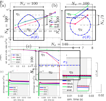
Figure 3: In (a) the match to Wulff shape for the model modifications in the base run as function of normalized strength of anisotropy $\Omega$. In (b) a detail of the phase field contours near the Wulff shape corner for simulation with $\Omega=7.5$.

Figure 4: Wulff shape shrinkage rate results. In (a) the mean shrinkage rate in the base run as function of normalized strength of anisotropy $\Omega$, in (b) and (c) there is time evolution of shrinkage rate for $\Omega=7.5$ in the base and IW/2 runs, respectively. The shaded areas in b) and c) indicate the time interval from which the mean shrinkage rate was computed.

The Figures 2a-2f visually compare the Wulff shapes obtained from simulation by the different models (in base run) to the analytic ones. As can be seen, the overall match is very good in all the three models, although a rather round contour near the corners in strong-anisotorpy Wulff shapes are observed (this is more apparent in Figure 3b, which shows detail of the contours near a corner for $\Omega=7.5$). That was expected, as no special finite difference scheme was used near corners (in [14] a one-sided finite difference scheme was proposed to avoid corners rounding).

Figure 3a, shows the match to Wulff shape as function of normalized strength of anisotropy $\Omega$ in the base run. As can be seen, the IWvG model slightly outperformed the other two in strong anisotropies because it was able to resolve the corners the best (see Figure 3b). However, when the interface width was halved in the IW/2 run, all the models performed nearly equally well because with smaller interface width the rounding near the corners was reduced. Interestingly, the IWvG model performed comparably in the IW/2 and base runs, which is in contrast to IWc and IWvK, which improved markedly with narrower interface width.
The best results in match to Wulff shape were obtained in the 14IWpts run with IWvG model. IWc and IWvK models performed comparably in the 14IWpts and IW/2 runs.

The mean shrinkage rates of the Wulff shapes as function of strength of anisotropy are in Figure 4a for the base run. At first sight, all the models perform comparably well, following the analytical prediction within an absolute error of 3 %. The Figures 4b and 4c show the time evolution of shrinkage rate with $\Omega=7.5$ in the base and IW/2 runs, respectively. It can be seen that despite the mean shrinkage rates being near the prediction, in the base run, the shrinkage rate of IWvG model did not converge to the analytic prediction (see the inset of Figure 4b, where the IWvG curve clearly declines). In the IW/2 run the IWvG model did converge close to the anaytic shrinkage rate (see also the inset of Figure 4c) and all the mean values are a little closer than in the base run. Note that in the IWvG model the lowest-energy interface has the widest interface width and that the cornered Wulff shape contains only interface orientations with lower energy. For this reason it required narrower interface width to reach constant shrinkage rate.

The relative error in mean shrinkage rate obtained with this methodology was nearly the same in the base and IW/2 runs though (both within $\pm 3\,\%$). Apparently, the difference is that with narrower interface the attained shrinkage rate is more steady. Additional run with even finer grid was carried out and no improvement in the mean values of shrinkage rates was observed. It can thus be concluded that the methodology is robust enough to assess the shrinkage rate even in the domain 100x100 (i.e. base run).

In addition to the four simulation runs discussed so far, the Wulff shapes simulations were re-run also with 4 and 5 points in the interface. The match to Wulff shape was worse than with 7 or 14 points, but the shapes were resolved qualitatively well regardless. The shrinkage rates were smaller than expected though, due to grid pinning. Seven points in the interface were thus confirmed as a reasonable value for the validations and practical simulations.

No significant effect of interface width scaling in the run 1000IW was found.

V.2 Kinetically compensated anisotropic circle shrinkage

Figure 5: Results for kinetically compensated anisotropic shrinkage. In (a) the match to circle for the base run, in (b) the mean shrinkage rate for 14IWpts run, in (c) and (d) the shrinkage rate time evolution in simulation with $\Omega=0.9$ in the base run and 14IWpts runs, respectively.

The quantified match to the circle and the mean shrinkage rate as functions of strength of anisotropy $\Omega$ are in Figures 5a and 5b, respectively (results of the base run showed). All models and runs retained the initial circle well or up to excellent geometrical match. Nevertheless, the IWvG model gave the best results, except for the strongest anisotropy, where the IWvK model was better. Only minor improvement in the match was achieved in the IW/2 run when compared to the base run. As with Wulff shapes simulations, the best match was obtained in the 14IWpts run, which also exhibited the best mean shrinkage rates (for all the three models).
The relative error in shrinkage rates in Figure 5b shows slightly decreasing trend with $\Omega$ for IWc and IWvG models (i.e. slowing down). The values of IWvK model were not affected and were constant. Apparently, the symmetric profiles of IWvK model provide an advantage for preserving the expected kinetics in simulations with strong kinetic anisotropy.
Time evolution of shrinkage rate for the strongest considered anisotropy (i.e. $\Omega=0.9$) in Figures 5c and 5d (base and 14IWpts runs, respectively), shows that in both runs the lines slightly diverge (this being applicable to all $\Omega$s). The convergence was better in IW/2 run, but the mean shrinkage rates were worse than in the 14IWpts run.

Apparently, optimal results would be obtained here with more points than 7 in the interface and with smaller interface-width-to-circle ratio than in the base run and 14IWpts runs. However, as noted earlier, the kinetic anisotropy is very strong in the case of $\Omega=0.9$. For weaker anisotorpy the discussed effects are less pronounced and there is little difference in the shrinkage rates among the models.

There was no significant difference between the results of base and 1000IW runs.

Figure 6: Triple junction angles. In a) the two methods for angles determination are illustrated (points fitted by straight lines in red and those fitted by circular arc in green). Subfigures b)-d) show the simulation results for different models, these being: in b) IWc, in c) IWvG and in d) IWvK. The hollow symbols correspond to the the angles determined by arc fitting and crosses to the lines fitting.

V.3 Equilibrium triple junction angles

Figures 6b-6d show the simulation results from the triple junction simulations as function of $\sigma_{1}/\sigma_{2}$. Neither of IWc or IWvK models show good agreement to Young’s law when deviating farther from an isotropic system (which has ratio $\sigma_{1}/\sigma_{2}=1$). The model IWvG, on the other hand, always shows very good agreement in at least one of the fitting methods along the whole range of probed ratios of interface energies. With $\sigma_{1}/\sigma_{2}$ closer to 2 in IWvG modification, the grains shape was slightly elongated in the vertical direction, resulting in too small radius of the fitted arcs to cross in the triple junction. The angles could not be determined this way then and the linear fit is more reliable.
For the ratios approximately $\sigma_{1}/\sigma_{2}\leq 0.45$ the IWc model behaves non-physically. The triple junction was observed to move in the opposite than expected direction (i.e. upwards, as if the triple junction angle was larger then 180°). The overall shape of contours was not as in Figure 6a because the green arcs curved in the other way. In IWvK this behavior was not observed, but the Young’s law is not followed. Qualitative explanation is that the IWc and IWvK models are not fully variational.
No significant change was observed in the results of the triple junction angles in runs IW/2, 14IWpts or 1000IW when compared to the base run. Quality of the results is thus not improved when more points in the interface than 7 are used. Also it implies, that the model behavior (for all parameters assignment strategies) is not affected by reducing the interface-width-to-feature ratio or the interface width scaling. The latter confirms that the model is quantitative.

VI Conclusions

This paper presented a quantitative methodology for assessment of the anisotropic curvature driving force in phase field method. It was demonstrated in comparison of three different modifications of a multi-phase field model. The match to the expected shape and the shrinkage rate were quantified in two different benchmark problems. The methodology was sensitive enough to capture differences between the model modifications and is suitable for validation and benchmarking of different models and numerical solvers.

The overall performance of the three model modifications in the benchmarks was comparable. Both match to the steady-state shapes and the shrinkage rates followed the expected results as in the anisotropic mean curvature flow. However, a significant difference was noted in a supplementary benchmark simulation where triple junction angles were measured. It was observed that only the IWvG model modification (with only the parameter $\gamma$ anisotropic) reproduced the triple junction angles in the full interval 0.13-2 of $\sigma_{1}/\sigma_{2}$, whereas IWc and IWvK modifications failed for ratios farther from 1. It is noted that these two modifications were not fully variational in order to avoid ghost phases, whereas IWvG is fully variational and yet the ghost phases do not appear.

Even though the triple junction benchmark did not involve interfaces with inclination-dependent interface energies, one conclusion can be made about that case regardless. As the IWc and IWvK were shown unreliable in the simpler pair-wise isotropic case, there is no reason why they should be reliable in the more complicated one. Further development and validations should thus focus on the IWvG model modification.

No results were significantly affected by the interface width scaling. Also, it was confirmed that 7 points in the interface were sufficient for retaining the expected kinetics in most cases, unless the inclination dependence of the kinetic coefficient was very strong.

The results in this paper are reproducible with codes provided in the data set [25].

VII Acknowledgements

The authors acknowledge the support of European Research Council (ERC) under the European Union’s Horizon 2020 research and innovation program (INTERDIFFUSION, Grant Agreement No. 714754).

References

- Jokisaari et al. [2017] A. Jokisaari, P. Voorhees, J. Guyer, J. Warren, and O. Heinonen, Benchmark problems for numerical implementations of phase field models, Computational Materials Science 126, 139 (2017).
- Olmsted et al. [2009] D. L. Olmsted, S. M. Foiles, and E. A. Holm, Survey of computed grain boundary properties in face-centered cubic metals: I. Grain boundary energy, Acta Materialia 57, 3694 (2009).
- Bulatov et al. [2014] V. V. Bulatov, B. W. Reed, and M. Kumar, Grain boundary energy function for fcc metals, Acta Materialia 65, 161 (2014).
- Garcke et al. [1999] H. Garcke, B. Stoth, and B. Nestler, Anisotropy in multi-phase systems: a phase field approach, Interfaces and Free Boundaries 1, 175 (1999).
- Tóth et al. [2015] G. I. Tóth, T. Pusztai, and L. Gránásy, Consistent multiphase-field theory for interface driven multidomain dynamics, Physical Review B - Condensed Matter and Materials Physics 92, 1 (2015), arXiv:1508.04311 .
- Salama et al. [2020] H. Salama, J. Kundin, O. Shchyglo, V. Mohles, K. Marquardt, and I. Steinbach, Role of inclination dependence of grain boundary energy on the microstructure evolution during grain growth, Acta Materialia 188, 641 (2020).
- Kazaryan et al. [2000] A. Kazaryan, Y. Wang, and S. Dregia, Generalized phase-field model for computer simulation of grain growth in anisotropic systems, Physical Review B - Condensed Matter and Materials Physics 61, 14275 (2000), arXiv:9912044 [cond-mat] .
- Wendler et al. [2011] F. Wendler, C. Mennerich, and B. Nestler, A phase-field model for polycrystalline thin film growth, Journal of Crystal Growth 327, 189 (2011).
- Tschukin et al. [2017] O. Tschukin, A. Silberzahn, M. Selzer, P. G. K. Amos, D. Schneider, and B. Nestler, Concepts of modeling surface energy anisotropy in phase ‑ field approaches, Geothermal Energy 10.1186/s40517-017-0077-9 (2017).
- Fleck et al. [2011] M. Fleck, L. Mushongera, D. Pilipenko, K. Ankit, and H. Emmerich, On phase-field modeling with a highly anisotropic interfacial energy, The European Physical Journal Plus 126, 95 (2011).
- Kobayashi [1993] R. Kobayashi, Modeling and numerical simulations of dendritic crystal growth, Physica D 63, 410 (1993).
- McFadden et al. [1993] G. B. McFadden, A. A. Wheeler, R. J. Braun, S. R. Coriell, and R. F. Sekerka, Phase-field models for anisotropic interfaces, Physical Review E 48, 2016 (1993).
- Taylor and Cahn [1998] J. E. Taylor and J. W. Cahn, Diffuse interfaces with sharp corners and facets: Phase field models with strongly anisotropic surfaces, Physica D: Nonlinear Phenomena 112, 381 (1998).
- Eggleston et al. [2001] J. Eggleston, G. McFadden, and P. Voorhees, A phase-field model for highly anisotropic interfacial energy, Physica D: Nonlinear Phenomena 150, 91 (2001).
- Wheeler [2006] A. A. Wheeler, Phase-field theory of edges in an anisotropic crystal, Proceedings of the Royal Society A: Mathematical, Physical and Engineering Sciences 462, 3363 (2006).
- Ma et al. [2006] N. Ma, Q. Chen, and Y. Wang, Implementation of high interfacial energy anisotropy in phase field simulations, Scripta Materialia 54, 1919 (2006).
- Torabi et al. [2009] S. Torabi, J. Lowengrub, A. Voigt, and S. Wise, A new phase-field model for strongly anisotropic systems, Proceedings of the Royal Society A: Mathematical, Physical and Engineering Sciences 465, 1337 (2009).
- Moelans et al. [2008] N. Moelans, B. Blanpain, and P. Wollants, Quantitative analysis of grain boundary properties in a generalized phase field model for grain growth in anisotropic systems, Physical Review B - Condensed Matter and Materials Physics 78, 10.1103/PhysRevB.78.024113 (2008).
- Bellettini and Paolini [1996] G. Bellettini and M. Paolini, Anisotropic motion by mean curvature in the context of finsler geometry, Hokkaido Mathematical Journal 25, 537 (1996).
- Beneš [2003] M. Beneš, Diffuse-interface treatment of the anisotropic mean-curvature flow, Applications of Mathematics 48, 437 (2003).
- Miyoshi et al. [2020] E. Miyoshi, T. Takaki, M. Ohno, and Y. Shibuta, Accuracy evaluation of phase-field models for grain growth simulation with anisotropic grain boundary properties, ISIJ International 60, 160 (2020).
- Moelans et al. [2010] N. Moelans, F. Spaepen, and P. Wollants, Grain growth in thin films with a fibre texture studied by phase-field simulations and mean field modelling, Philosophical Magazine 90, 501 (2010).
- Ravash et al. [2017] H. Ravash, J. Vleugels, and N. Moelans, Three-dimensional phase-field simulation of microstructural evolution in three-phase materials with different interfacial energies and different diffusivities, Journal of Materials Science 52, 13852 (2017).
- Minar and Moelans [2022] M. Minar and N. Moelans, See Supplemental material at xxx for the best practices in parameters determination in Moelans’ model and for further details on the implementation., Phys.Rev.Mat. (2022).
- Minar [2022] M. Minar, Benchmarking of different strategies to include anisotropy in a curvature-driven multi-phase-field model, Mendeley Data, v2 10.17632/5wrv3ky9pp.2 (2022).
- Burton et al. [1951] W. K. Burton, N. Cabrera, and F. C. Frank, The Growth of Crystals and the Equilibrium Structure of their Surfaces, Philosophical Transactions of the Royal Society A: Mathematical, Physical and Engineering Sciences 243, 299 (1951).
- Kobayashi and Giga [2001] R. Kobayashi and Y. Giga, On anisotropy and curvature effects for growing Crystals, Japan Journal of Industrial and Applied Mathematics 18, 207 (2001).
- Moelans et al. [2009] N. Moelans, F. Wendler, and B. Nestler, Comparative study of two phase-field models for grain growth, Computational Materials Science 46, 479 (2009).
- Alt et al. [2004] H. Alt, C. Knauer, and C. Wenk, Comparison of Distance Measures for Planar Curves, Algorithmica 38, 45 (2004).
- Li Zhu and Chun-qiang Zhu [2014] Li Zhu and Chun-qiang Zhu, Application of Hausdorff distance in image matching, in 2014 IEEE Workshop on Electronics, Computer and Applications, 3 (IEEE, 2014) pp. 97–100.
- Porter et al. [2009] D. A. Porter, K. E. Easterling, and K. E. Easterling, Phase Transformations in Metals and Alloys (Revised Reprint), 3rd ed. (CRC Press, 2009).