Energy stability of variable-step L1-type schemes for time-fractional Cahn-Hilliard model

Abstract

The positive definiteness of discrete time-fractional derivatives is fundamental to the numerical stability (in the energy sense) for time-fractional phase-field models. A novel technique is proposed to estimate the minimum eigenvalue of discrete convolution kernels generated by the nonuniform L1, half-grid based L1 and time-averaged L1 formulas of the fractional Caputo’s derivative. The main discrete tools are the discrete orthogonal convolution kernels and discrete complementary convolution kernels. Certain variational energy dissipation laws at discrete levels of the variable-step L1-type methods are then established for time-fractional Cahn-Hilliard model. They are shown to be asymptotically compatible, in the fractional order limit $\alpha\rightarrow 1$, with the associated energy dissipation law for the classical Cahn-Hilliard equation. Numerical examples together with an adaptive time-stepping procedure are provided to demonstrate the effectiveness of the proposed methods.
Keywords:   time-fractional Cahn-Hilliard model; variable-step L1-type formulas; discrete convolution tools; positive definiteness; variational energy dissipation law
AMS subject classiffications.   35Q99, 65M06, 65M12, 74A50

1 Introduction

In this paper, we study the energy stability of three nonuniform L1-type approximations for the time-fractional Cahn-Hilliard (TFCH) model[23]

$$\partial_{t}^{\alpha}\Phi=\kappa\Delta\mu\quad\text{with}\quad\mu=\tfrac{\delta E}{\delta\Phi}=f(\Phi)-\epsilon^{2}\Delta\Phi,$$ (1.1)

where the Ginzburg-Landau energy functional is given by [2],

$$E[\Phi]=\int_{\Omega}\Big{(}\frac{\epsilon^{2}}{2}\left|\nabla\Phi\right|^{2}+F(\Phi)\Big{)}\,\mathrm{d}\mathbf{x}.$$ (1.2)

Here, the real valued function $\Phi$ represents the concentration difference in a binary system, spatial domain $\mathbf{x}\in\Omega\subseteq\mathbb{R}^{2}$, $\epsilon>0$ is an interface width parameter, $\kappa>0$ is the mobility coefficient and the double-well potential $F(\Phi)=\frac{1}{4}\left(\Phi^{2}-1\right)^{2}$. The notation $\partial_{t}^{\alpha}:={}_{0}^{C}\!D_{t}^{\alpha}$ represents the Caputo’s fractional derivative of order $\alpha\in(0,1)$ with respect to $t$, defined by [18],

$$(\partial_{t}^{\alpha}v)(t):=(\mathcal{I}_{t}^{1-\alpha}v^{\prime})(t)\quad\text{where}\quad(\mathcal{I}_{t}^{\beta}v)(t):=\int_{0}^{t}\omega_{\beta}(t-s)v(s)\,\mathrm{d}{s},$$ (1.3)

and $\omega_{\beta}(t):=t^{\beta-1}/\Gamma(\beta)$ for $\beta>0$.

Throughout this paper, the periodic boundary conditions are adopted for simplicity. If the initial data is properly regular, the global existence of solutions of the TFCH equation (1.1) was established in [1]. Moreover, [1, Theorem 3.3] showed that the problem (1.1) has a unique solution and $\big{\|}\partial_{t}\Phi\big{\|}\leq C_{\Phi}t^{\alpha\nu/4-1}$ for $0<t\leq T$ if $\Phi_{0}\in\dot{H}^{\nu}(\Omega)\,(\nu\in[1,2])$. It reveals that the solution of the TFCH equation lacks the smoothness near the initial time while it would be smooth away from $t=0$, also see [22, 9, 14] and the references therein. In addition, the TFCH equation (1.1) conserves the initial volume $\big{(}\Phi(t),1\big{)}=\left(\Phi(0),1\right)$ for $t>0$ [23, Theorem 2.2]. Recently, Liao, Tang and Zhou [13] showed that the time-fractional phase field models preserve the following variational energy dissipation law,

$$\frac{\,\mathrm{d}\mathcal{E}_{\alpha}}{\,\mathrm{d}t}+\frac{\kappa}{2}\omega_{\alpha}(t)\big{\|}\nabla\mu\big{\|}^{2}\leq 0\quad\text{with}\quad\mathcal{E}_{\alpha}(t):=E(t)+\frac{\kappa}{2}\mathcal{I}_{t}^{\alpha}\big{\|}\nabla\mu\big{\|}^{2}\quad\text{for $t>0$},$$ (1.4)

where $(\cdot,\cdot)$ and $\left\|\cdot\right\|$ denote the $L^{2}(\Omega)$ inner product and the associated norm, respectively.

As pointed out in [13], compared with the global energy dissipation property in [23, 3], the time-fractional energy decaying law and the weighted energy dissipation law in [20, 21], the new law (1.4) seems to be naturally consistent with the standard energy dissipation law of the classical Cahn-Hilliard (CH) model in the sense that

$$\frac{\,\mathrm{d}\mathcal{E}_{\alpha}}{\,\mathrm{d}t}+\frac{\kappa}{2}\omega_{\alpha}(t)\big{\|}\nabla\mu\big{\|}^{2}\leq 0\quad\rightarrow\quad\frac{\,\mathrm{d}E}{\,\mathrm{d}t}+\kappa\big{\|}\nabla\mu\big{\|}^{2}\leq 0\qquad\text{as $\alpha\rightarrow 1$}.$$

Our aim of this paper is to develop numerical methods that preserve the variational energy dissipation law (1.4) at discrete time levels. For a given time $T>0$, consider a nonuniform time levels $0=t_{0}<t_{1}<\cdots<t_{k-1}<t_{k}<\cdots<t_{N}=T$ with the time-step sizes $\tau_{k}:=t_{k}-t_{k-1}$ for $1\leq k\leq N$. The maximum time-step size is denoted by $\tau:=\max_{1\leq k\leq N}\tau_{k}$ and the local time-step ratio $r_{k}:=\tau_{k}/\tau_{k-1}$ for $2\leq k\leq N$.

Given a grid function $\{v^{k}\}_{k=0}^{N}$, define the difference $\triangledown_{\!\tau}v^{k}:=v^{k}-v^{k-1}$ and $\partial_{\tau}v^{k}:=\triangledown_{\!\tau}v^{k}/\tau_{k}$ for $k\geq{1}$. Let $\Pi_{1,k}v$ denote the linear interpolant of a function $v$ with respect to the nodes $t_{k-1}$ and $t_{k}$, such that $\left(\Pi_{1,k}v\right)^{\prime}(t)=\triangledown_{\!\tau}v^{k}/\tau_{k}$ for $t\in(t_{k-1},t_{k})$. We will investigate three L1-type formulas on nonuniform meshes. The first one is the standard L1 approximation [14],

$$(\partial_{\tau}^{\alpha}v)^{n}:=\int_{0}^{t_{n}}\omega_{1-\alpha}(t_{n}-s)(\Pi_{1}v)^{\prime}(s)\,\mathrm{d}{s}\triangleq\sum_{k=1}^{n}a_{n-k}^{(n)}\triangledown_{\!\tau}v^{k},$$ (1.5)

where the associated discrete L1 kernels $a_{n-k}^{(n)}$ are defined by

$$a_{n-k}^{(n)} :=\frac{1}{\tau_{k}}\int_{t_{k-1}}^{t_{k}}\omega_{1-\alpha}(t_{n}-s)\,\mathrm{d}{s}$$

$$=\frac{1}{\tau_{k}}\left[\omega_{2-\alpha}(t_{n}-t_{k-1})-\omega_{2-\alpha}(t_{n}-t_{k})\right]\quad\text{for $1\leq{k}\leq{n}$}.$$ (1.6)

The second formula, named L1_h, is defined at the half-grid point $t_{n-\frac{1}{2}}$,

$$(\partial_{\mathrm{h}\tau}^{\alpha}v)^{n-\frac{1}{2}}:=\int_{0}^{t_{n-\frac{1}{2}}}\omega_{1-\alpha}(t_{n-\frac{1}{2}}-s)(\Pi_{1}v)^{\prime}(s)\,\mathrm{d}{s}\triangleq\sum_{k=1}^{n}a_{n-k}^{(\mathrm{h},n)}\triangledown_{\!\tau}v^{k},$$ (1.7)

where the corresponding discrete L1_h kernels $a_{n-k}^{(\mathrm{h},n)}$ are given by

$$a_{n-k}^{(\mathrm{h},n)}:=\frac{1}{\tau_{k}}\int_{t_{k-1}}^{\min\{t_{k},t_{n-\frac{1}{2}}\}}\omega_{1-\alpha}(t_{n-\frac{1}{2}}-s)\,\mathrm{d}{s}\quad\text{for $1\leq k\leq n$}.$$ (1.8)

The third one, called L1_a, is an averaged version of L1 formula (1.5) at $t_{n-\frac{1}{2}}$, that is,

$$(\partial_{\mathrm{a}\tau}^{\alpha}v)^{n-\frac{1}{2}}:=\frac{1}{2}\left[(\partial_{\tau}^{\alpha}v)^{n}+(\partial_{\tau}^{\alpha}v)^{n-1}\right]\triangleq\sum_{k=1}^{n}a_{n-k}^{(\mathrm{a},n)}\triangledown_{\!\tau}v^{k},$$ (1.9)

where the corresponding discrete L1_a kernels $a_{n-k}^{(\mathrm{a},n)}$ are defined by

$$a_{0}^{(\mathrm{a},n)}:=\frac{1}{2}a_{0}^{(n)}\quad\text{and}\quad a_{n-k}^{(\mathrm{a},n)}:=\frac{1}{2}\big{(}a_{n-k}^{(n)}+a_{n-1-k}^{(n-1)}\big{)}\quad\text{for $1\leq k\leq n-1$}.$$ (1.10)

By means of the above three L1-type formulas (1.8)-(1.10), we consider the following semi-discrete time-stepping methods for the TFCH model:

• The backward Euler-type L1 scheme

  $$\left(\partial_{\tau}^{\alpha}\phi\right)^{n}=\kappa\Delta\mu^{n}\quad\text{with}\quad\mu^{n}=f(\phi^{n})-\epsilon^{2}\Delta\phi^{n},\quad n\geq 1;$$ (1.11)

• The Crank-Nicolson-type L1_h scheme

  $$\left(\partial_{\mathrm{h}\tau}^{\alpha}\phi\right)^{n-\frac{1}{2}}=\kappa\Delta\mu^{n-\frac{1}{2}}\quad\text{with}\quad\mu^{n-\frac{1}{2}}=f(\phi)^{n-\frac{1}{2}}-\epsilon^{2}\Delta\phi^{n-\frac{1}{2}},\quad n\geq 1;$$ (1.12)

• The Crank-Nicolson-type L1_a scheme

  $$\left(\partial_{\mathrm{a}\tau}^{\alpha}\phi\right)^{n-\frac{1}{2}}=\kappa\Delta\mu^{n-\frac{1}{2}}\quad\text{with}\quad\mu^{n-\frac{1}{2}}=f(\phi)^{n-\frac{1}{2}}-\epsilon^{2}\Delta\phi^{n-\frac{1}{2}},\quad n\geq 1,$$ (1.13)

where the averaged difference operator $\phi^{n-\frac{1}{2}}:=(\phi^{n}+\phi^{n-1})/2$ and $f(\phi)^{n-\frac{1}{2}}$ is a second-order approximation [13, Appendix A] of the nonlinear term $f(\phi)$

$$f(\phi)^{n-\frac{1}{2}}:=\frac{1}{3}\left(\phi^{n}\right)^{3}+\frac{1}{2}\phi^{n}\left(\phi^{n-1}\right)^{2}+\frac{1}{6}\left(\phi^{n-1}\right)^{3}-\phi^{n-\frac{1}{2}}.$$

Without losing generality, we consider periodic boundary conditions with a proper initial data $\phi^{0}(\mathbf{x})$. Our analysis can be extended in a straightforward way to the fully discrete numerical schemes with some appropriate spatial discretization preserving the discrete integration-by-parts formulas, such as the Fourier pseudo-spectral method [5, 4] used in our experiments.

A major hindrance in establishing the discrete energy stability for the time-fractional phase field models is the positive definiteness of the following real quadratic form with respect to the convolution kernels $a_{n-j}^{(n)}$ (in a general sense) arising from variable-step time approximations

$${\color[rgb]{0,0,1}2}\sum_{k=1}^{n}w_{k}\sum_{j=1}^{k}a_{k-j}^{(k)}w_{j}\quad\text{for any nonzero sequence $\{w_{1},w_{2},\cdots,w_{n}\}$}.$$ (1.14)

On the uniform time mesh with $a_{j}^{(n)}=a_{j}$, López-Marcos [17, Proposition 5.2] gave some sufficient but algebraic conditions to check the desired property,

$$a_{j}\geq 0,\quad a_{j-1}\geq a_{j}\quad\text{and}\quad a_{j-1}-a_{j}\geq a_{j}-a_{j+1}.$$ (1.15)

The positive, decreasing and convex criteria have been widely used to establish the stability and convergence results for integro-differential and time-fractional differential problem, such as [7, Lemma 2.6] for a discrete (global) energy law for the time-fractional Allen-Cahn model. Very recently, Karaa [10] presented some criteria ensuring the positivity of the real quadratic form (1.14) for some commonly used numerical methods, including the convolution quadrature method and L1 formula.

It is worthwhile noting that the criterion (1.15) may fail to verify the desired positive definiteness of the real quadratic form (1.14) for the variable-step time-stepping methods, such as the nonuniform L1 method [7, Remark 1]. Also, the technique of completely monotone sequence in [10] may not be applied to the nonuniform case directly. Recently, Liao et. al. [12] proposed another class of sufficient but easy-to-check conditions (for general discrete kernels)

$$a_{j-1}^{(n)}\geq a_{j}^{(n)}>0,\quad a_{j-1}^{(n-1)}>a_{j}^{(n)}\quad\text{and}\quad a_{j-1}^{(n-1)}a_{j+1}^{(n)}\geq a_{j}^{(n-1)}a_{j}^{(n)}.$$ (1.16)

The main theorem of [12, Theorem 1.1] ensures that the positive, decreasing and convex criteria (1.16) are sufficient for the positive definiteness of associated quadratic form resulting from a general class of discrete convolution approximations. By a careful verification of the sufficient condition (1.16), the positive definiteness of the nonuniform L1 kernels $a_{n-k}^{(n)}$ was verified in [12, Proposition 4.1]. As a direct application, the stabilized semi-implicit scheme was shown to preserve the global energy stability on arbitrary meshes, see [12, Proposition 4.2].

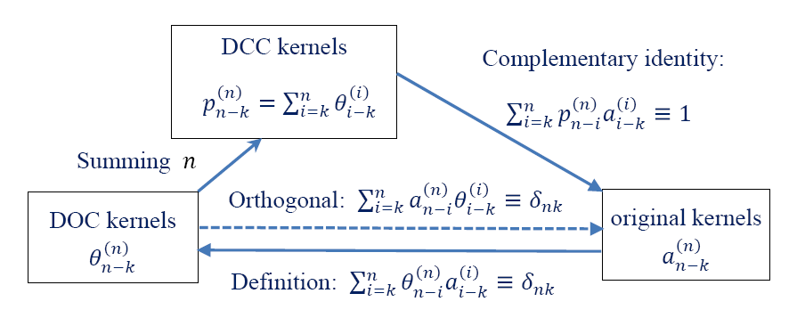
Figure 1: The relationship diagram of DOC, DCC and original kernels.

However, the positive definiteness property in [12, Proposition 4.1] may not be sufficient to build up a discrete energy stability for some fully implicit methods, such as the implicit L1 scheme (2.11) in [7]. By means of some new discrete tools, the recent work [15] filled this gap for the time-fractional Allen-Cahn model by demonstrating that the implicit L1 scheme preserving the discrete variational energy law (1.4) on arbitrary time meshes. One of the key tools is the discrete orthogonal convolution (DOC) kernels defined by the following recursive procedure

$$\theta_{0}^{(n)}:=\frac{1}{a_{0}^{(n)}}\quad\mathrm{and}\quad\theta_{n-k}^{(n)}:=-\frac{1}{a_{0}^{(k)}}\sum_{j=k+1}^{n}{\theta_{n-j}^{(n)}}a_{j-k}^{(j)}\quad\text{for $1\leq k\leq n-1$}.$$ (1.17)

It is easy to check that the DOC kernels $\theta_{n-k}^{(n)}$ satisfy the discrete orthogonal identity

$$\sum_{j=k}^{n}\theta_{n-j}^{(n)}a_{j-k}^{(j)}\equiv\delta_{nk}\quad\text{for $1\leq k\leq n$,}$$ (1.18)

where $\delta_{nk}$ is the Kronecker delta symbol. Furthermore, another useful discrete analysis tool is the so-called discrete complementary convolution (DCC) kernels introduced by means of the DOC kernels $\theta_{n-k}^{(n)}$, see [12, Subsection 2.2],

$$p_{n-k}^{(n)}:=\sum_{j=k}^{n}\theta_{j-k}^{(j)}\quad\text{such that}\quad\sum_{j=k}^{n}p_{n-j}^{(n)}a_{j-k}^{(j)}\equiv 1\quad\text{for $1\leq k\leq n$}.$$ (1.19)

The interplay relationship of the mentioned DOC and DCC kernels together with the original kernels is summarized in Figure 1, also see [12, Figure 1].

In this paper, we investigate the positive definiteness of the L1-type kernels from the L1-type approximations (1.5), (1.7) and (1.9) of the Caputo derivative, and explore the energy stability of the associated numerical methods (1.11)-(1.13). Some novel discrete convolution inequalities with respect to the L1 and L1_h kernels are established in Theorems 2.1 and 2.2, respectively. Let $\lambda_{\min}$ be the minimum eigenvalue of the real quadratic form (matrix) involving the L1 kernels ($\lambda_{\min}^{(\mathrm{h})}$ and $\lambda_{\min}^{(\mathrm{a})}$ of L1_h kernels and L1_a kernels are defined similarly). Subsection 2.1 obtains the certain lower bound of the minimum eigenvalue. To the best of our knowledge, such estimate of the minimum eigenvalue on arbitrary time meshes is considered at the first time. The positive definiteness of the L1_h kernels (1.8) is also verified in subsection 2.2 although the first two kernels lose their monotonicity, see Table 1 which collects some related properties of the underlying discrete kernels. However, the positive definite property of the averaged L1_a kernels (1.10) is still undetermined, see more details in subsection 2.3.

Table 1: Kernels properties of L1-type formulas on nonuniform time meshes.

  Theoretical properties L1 kernels (1) L1_h kernels (1.8) L1_a kernels (1.10) Positivity $a_{j}^{(n)}>0$ $a_{j}^{(\mathrm{h},n)}>0$ $a_{j}^{(\mathrm{a},n)}>0$ Monotonicity strict decreasing $a_{0}^{(\mathrm{h},n)}\ngeq a_{1}^{(\mathrm{h},n)}$ $a_{0}^{(\mathrm{a},n)}\ngeq a_{1}^{(\mathrm{a},n)}$ Positive definiteness (with eigenvalues $\lambda$) $\lambda_{\min}\geq\min\limits_{1\leq k\leq n}a_{0}^{(k)}$ $\lambda_{\min}^{(\mathrm{h})}>0$ undetermined  

Then we show in Theorems 3.4 and 3.4 that the proposed numerical schemes (1.11)-(1.12) preserve the variational energy dissipation law (1.4) on arbitrary time meshes. These discrete energy laws are shown to be asymptotically compatible with the classical energy dissipation laws as the fractional order $\alpha\rightarrow 1$, see Remarks 2-4.

The rest of this paper is organized as follows. In section 2, the positive definiteness of the suggested L1-type formulas is investigated. Section 3 establishes the discrete energy dissipation laws of the L1-type time-stepping schemes. Numerical examples are presented in section 4 to confirm our theoretical findings.

2 Positive definiteness of L1-type formulas

2.1 Positive definiteness of L1 kernels

It follows from [12, Proposition 4.1] that the discrete L1 kernels $a_{n-k}^{(n)}$ satisfy the criteria (1.16) so that the following result holds according to [12, Theorem 1.1].

Lemma 2.1.

The L1 kernels $a_{j}^{(n)}$ in (1) are positive definite in the sense that

$${\color[rgb]{0,0,1}2}\sum_{k=1}^{n}w_{k}\sum_{j=1}^{k}a_{k-j}^{(k)}w_{j}>0\quad\text{for any nonzero sequence $\{w_{1},w_{2},\cdots,w_{n}\}$}.$$ (2.1)

In what follows, we improve Lemma 2.1 by presenting a lower bound $\sigma_{\text{L1}}>0$ for the minimum eigenvalue of the associated quadratic form in the sense that

$${\color[rgb]{0,0,1}2}\sum_{k=1}^{n}w_{k}\sum_{j=1}^{k}a_{k-j}^{(k)}w_{j}\geq\sigma_{\text{L1}}\sum_{k=1}^{n}w_{k}^{2}.$$ (2.2)

To this end, we first list some properties of the DOC kernels $\theta_{n-k}^{(n)}$ defined in (1.17), and the DCC kernels $p_{n-k}^{(n)}$ defined in (1.19), see [12, Lemmas 2.3 and 2.5].

Lemma 2.2.

For any $n\geq 2$, the DOC kernels $\theta_{n-k}^{(n)}$ in (1.17) satisfy

$$\theta_{0}^{(n)}>0\quad\text{and}\quad\theta_{n-k}^{(n)}<0\quad\text{for $1\leq k\leq n-1$};\quad\text{but}\quad\sum_{k=1}^{n}\theta_{n-k}^{(n)}>0;$$

and the DCC kernels $p_{n-k}^{(n)}$ in (1.19) satisfy

$$p_{n-k}^{(n)}=\sum_{j=k}^{n}\theta_{j-k}^{(j)}\geq 0\quad\text{for $1\leq k\leq n$.}$$

According to the definition (1.19), one can find that the DOC kernels $\theta_{n-k}^{(n)}$ and the DCC kernels $p_{n-k}^{(n)}$ satisfy the following relationship

$$\theta_{0}^{(n)}=p_{0}^{(n)}\quad\text{and}\quad\theta_{n-k}^{(n)}=p_{n-k}^{(n)}-p_{n-1-k}^{(n-1)}\quad\text{for $1\leq k\leq n-1$}.$$ (2.3)

Then we have the following positive definiteness result for the DOC kernels $\theta_{n-k}^{(n)}$.

Lemma 2.3.

For any real vector sequence $\{w_{k}\}_{k=1}^{n}$, it holds that

$$2w_{k}\sum_{j=1}^{k}\theta_{k-j}^{(k)}w_{j}\geq\sum_{j=1}^{k}p_{k-j}^{(k)}w_{j}^{2}-\sum_{j=1}^{k-1}p_{k-1-j}^{(k-1)}w_{j}^{2}+\frac{1}{\theta_{0}^{(k)}}\Big{(}\sum_{j=1}^{k}\theta_{k-j}^{(k)}w_{j}\Big{)}^{2}\quad\text{for $k\geq 1$,}$$

so that the DOC kernels $\theta_{n-k}^{(n)}$ are positive definite in the sense that

$$2\sum_{k=1}^{n}w_{k}\sum_{j=1}^{k}\theta_{k-j}^{(k)}w_{j}\geq\sum_{k=1}^{n}p_{n-k}^{(n)}w_{k}^{2}+\sum_{k=1}^{n}\frac{1}{\theta_{0}^{(k)}}\Big{(}\sum_{j=1}^{k}\theta_{k-j}^{(k)}w_{j}\Big{)}^{2}>0\quad\text{if $w_{k}\not\equiv 0$.}$$

Proof.

The first inequality can be verified by the proof of [15, Lemma 2.4]. Summing up this inequality from $k=1$ to $n$, one gets the claimed second inequality and the proof is completed. ∎

Theorem 2.1.

For any real vector sequence $\{w_{k}\}_{k=1}^{n}$, it holds that

$$2w_{k}\sum_{j=1}^{k}a_{k-j}^{(k)}w_{j}\geq a_{0}^{(k)}w_{k}^{2}+\sum_{j=1}^{k}p_{k-j}^{(k)}\Big{(}\sum_{\ell=1}^{j}a_{j-\ell}^{(j)}w_{\ell}\Big{)}^{2}-\sum_{j=1}^{k-1}p_{k-1-j}^{(k-1)}\Big{(}\sum_{\ell=1}^{j}a_{j-\ell}^{(j)}w_{\ell}\Big{)}^{2}$$

for $k\geq 1$, so that the L1 kernels $a_{n-k}^{(n)}$ in (1) are positive definite in the sense that

$$2\sum_{k=1}^{n}w_{k}\sum_{j=1}^{k}a_{k-j}^{(k)}w_{j}\geq\sum_{k=1}^{n}a_{0}^{(k)}w_{k}^{2}+\sum_{k=1}^{n}p_{n-k}^{(n)}\Big{(}\sum_{j=1}^{k}a_{k-j}^{(k)}w_{j}\Big{)}^{2}>0\quad\text{if $w_{k}\not\equiv 0$.}$$

Proof.

For any fixed index $n\geq 1$ and any real vector sequence $\{w_{k}\}_{k=1}^{n}$, we introduce an auxiliary sequence $\{v_{k}\}_{k=1}^{n}$ by means of the original kernels $a_{j-k}^{(j)}$ as follows

$$v_{j}:=\sum_{k=1}^{j}a_{j-k}^{(j)}w_{k}\quad\text{for $1\leq j\leq n$.}$$ (2.4)

Multiplying both sides of the equality (2.4) by $\theta_{j-k}^{(j)}$ and summing up from $k=1$ to $j$ give

$$\sum_{k=1}^{j}\theta_{j-k}^{(j)}v_{k}=\sum_{k=1}^{j}\theta_{j-k}^{(j)}\sum_{\ell=1}^{k}a_{k-\ell}^{(k)}w_{\ell}=\sum_{\ell=1}^{j}w_{\ell}\sum_{k=\ell}^{j}\theta_{j-k}^{(j)}a_{k-\ell}^{(k)}=w_{j}\quad\text{for $1\leq j\leq n$,}$$ (2.5)

where the discrete orthogonal identity (1.18) has been used in the last step. According to the first inequality in Lemma 2.3 and the fact $a_{0}^{(k)}=1/\theta_{0}^{(k)}$ from (1.17), one has

$$2v_{k}\sum_{j=1}^{k}\theta_{k-j}^{(k)}v_{j}\geq\sum_{j=1}^{k}p_{k-j}^{(k)}v_{j}^{2}-\sum_{j=1}^{k-1}p_{k-1-j}^{(k-1)}v_{j}^{2}+a_{0}^{(k)}\Big{(}\sum_{j=1}^{k}\theta_{k-j}^{(k)}v_{j}\Big{)}^{2}\quad\text{for $k\geq 1$,}$$

which directly leads to the claimed first inequality by the above relationships (2.4)-(2.5). ∎

Theorem 2.1 expresses the discrete convolution structure of the nonuniform L1 formula (1.5) with the original convolution kernels $a_{n-k}^{(n)}$ rather than the corresponding DOC kernels $\theta_{n-k}^{(n)}$. This form will be heuristic in treating other numerical Caputo derivatives, especially when the associated discrete kernels lose the monotonicity, see the L1_h kernels in next subsection. As a byproduct, this form updates Lemma 2.1 by presenting a lower bound

$$\sigma_{\text{L1}}:=\min_{1\leq k\leq n}a_{0}^{(k)}$$

for the minimum eigenvalue $\lambda_{\min}$ of the associated quadratic form. Table 2 tabulates the low bound $\sigma_{\text{L1}}$ and the minimum eigenvalue $\lambda_{\min}$ on the random time meshes with $T=1$ for three different fractional orders $\alpha$. As observed, $\sigma_{\text{L1}}$ is a delicate estimate of $\lambda_{\min}$, especially when the fractional order $\alpha$ is small. Table 3 also lists the comparsions on the graded mesh $t_{k}=T(k/N)^{\gamma}$, which was applied frequently in resolving the initial singularity [22, 9, 11].

Table 2: Comparisons of the bound $\sigma_{\text{L1}}$ and $\lambda_{\min}$ on random time meshes.

  $N$ $\alpha=0.1$ $\alpha=0.5$ $\alpha=0.9$ $\sigma_{\text{L1}}$ $\lambda_{\min}$ $\sigma_{\text{L1}}$ $\lambda_{\min}$ $\sigma_{\text{L1}}$ $\lambda_{\min}$ 100 1.53 1.72 7.73 12.37 33.57 65.85 200 1.65 1.84 11.19 17.91 65.35 128.74 400 1.76 1.97 15.83 24.99 121.98 239.22  

Table 3: Comparisons of the bound $\sigma_{\text{L1}}$ and $\lambda_{\min}$ for $\alpha=0.5$ on graded time meshes.

  $N$ $\gamma=1$ $\gamma=2$ $\gamma=4$ $\sigma_{\text{L1}}$ $\lambda_{\min}$ $\sigma_{\text{L1}}$ $\lambda_{\min}$ $\sigma_{\text{L1}}$ $\lambda_{\min}$ 100 11.28 17.16 8.00 12.36 5.68 8.92 200 15.96 24.26 11.30 17.36 8.01 12.43 400 22.57 34.31 15.97 24.44 11.30 17.42  

The sharpness of the bound $\sigma_{\text{L1}}$ can be also seen by comparing with a previous result in [23, Lemma 3.1] on the uniform grid. In this simple case, Theorem 2.1 shows $\sigma_{\text{L1}}=\frac{1}{\Gamma(2-\alpha){\tau}^{\alpha}}$, while Tang et al [23, Lemma 3.1] gave the following bound

$$\sigma_{*}:=\frac{1}{\tau^{\alpha}\Gamma(1-\alpha)}\big{(}\frac{2}{n+1}\big{)}^{\alpha}.$$

The current estimate $\sigma_{\text{L1}}$ is sharper than $\sigma_{*}$, that is,

$$\frac{\sigma_{\text{L1}}}{\sigma_{*}}=\frac{2^{-\alpha}}{1-\alpha}(n+1)^{\alpha}>(n+1)^{\alpha},$$

due to the fact $2^{-\alpha}>1-\alpha$ for $\alpha\in(0,1)$. Very recently, Karaa[10, Lemma 3.4] gave a new bound $\sigma_{\star}$ on the uniform mesh, that is,

$$\sigma_{\star}:=\frac{2\mathrm{Li}_{\alpha-1}(-1)}{(-1)\Gamma(2-\alpha)\tau^{\alpha}},$$

where the polylogarithm function $\mathrm{Li}_{\beta}(z):=\sum_{j=1}^{\infty}\frac{z^{j}}{j^{\beta}}$, which is well defined for $|z|<1$ and can be analytically extended to the split domain $\mathbb{C}\backslash[1,\infty)$. Actually, $\sigma_{\star}\geq\sigma_{\text{L1}}$ on the uniform mesh due to the fact $(-1)\mathrm{Li}_{\alpha-1}(-1)\geq 1/4$. It seems that the result of Theorem 2.1 still has a lot of room for improvement.

2.2 Positive definiteness of L1_h kernels

The L1_h kernels in (1.8) are different from the L1 kernels due to the lack of the monotonicity. Simple calculations show that the first two discrete L1_h kernels defined in (1.8) satisfy

$$a_{0}^{(\mathrm{h},n)}-a_{1}^{(\mathrm{h},n)}=a_{0}^{(\mathrm{h},n)}\Big{[}1+r_{n}-r_{n}^{\alpha}\big{(}r_{n}+2\big{)}^{1-\alpha}\Big{]}.$$

It is evident that $a_{0}^{(\mathrm{h},n)}>a_{1}^{(\mathrm{h},n)}$ as $\alpha\rightarrow 1$ and $a_{0}^{(\mathrm{h},n)}<a_{1}^{(\mathrm{h},n)}$ as $\alpha\rightarrow 0,$ i.e., the monotonously decreasing of the L1_h kernels $a_{j}^{(\mathrm{h},n)}$ loses for some fractional orders $\alpha\in(0,1)$. So the sufficient criterion (1.16) or [12, Theorem 1.1] can not be directly applied to confirm the positive definiteness of the discrete L1_h kernels $a_{j}^{(\mathrm{h},n)}$.

Further observations suggest that the desired monotonicity property can be attained by doubling the first kernel $a_{0}^{(\mathrm{h},n)}$. Actually, the inequality $1+\beta z>(1+z)^{\beta}$ holds for any $\beta\in(0,1)$ with respect to $z>0$ and then

$$2a_{0}^{(\mathrm{h},n)}-a_{1}^{(\mathrm{h},n)} =a_{0}^{(\mathrm{h},n)}\big{[}2+r_{n}-r_{n}^{\alpha}\big{(}r_{n}+2\big{)}^{1-\alpha}\big{]}$$

$$>a_{0}^{(\mathrm{h},n)}r_{n}\left[1+2(1-\alpha)/r_{n}-(1+2/r_{n})^{1-\alpha}\right]>0.$$ (2.6)

Accordingly, we introduce the following auxiliary kernels via the original L1_h kernels $a_{j}^{(\mathrm{h},n)}$,

$$\mathsf{a}_{0}^{(\mathrm{h},n)}:=2a_{0}^{(\mathrm{h},n)}\quad\text{and}\quad\mathsf{a}_{j}^{(\mathrm{h},n)}:=a_{j}^{(\mathrm{h},n)}\quad\text{for $1\leq j\leq n-1$.}$$ (2.7)

Lemma 2.4.

For any fixed $n\geq 2$, the auxiliary L1_h kernels $\mathsf{a}_{j}^{(\mathrm{h},n)}$ in (2.7) satisfy

$$\mathsf{a}_{j-1}^{(\mathrm{h},n)}\geq\mathsf{a}_{j}^{(\mathrm{h},n)}>0,\quad\mathsf{a}_{j-1}^{(\mathrm{h},n-1)}>\mathsf{a}_{j}^{(\mathrm{h},n)},\quad\mathsf{a}_{j-1}^{(\mathrm{h},n-1)}\mathsf{a}_{j+1}^{(\mathrm{h},n)}>\mathsf{a}_{j}^{(\mathrm{h},n-1)}\mathsf{a}_{j}^{(\mathrm{h},n)}.$$

Then the auxiliary L1_h kernels $\mathsf{a}_{j}^{(\mathrm{h},n)}$ are positive definite according to [12, Theorem 1.1].

Proof.

The positivity and the monotonous decreasing of $\mathsf{a}_{j}^{(\mathrm{h},n)}$ follow from the definition (2.7) and the integral mean value theorem immediately. Then, we consider the following sequence

$$\psi_{n-k}^{(\mathrm{h},n)}:=\frac{\mathsf{a}_{n-k}^{(\mathrm{h},n)}}{\mathsf{a}_{n-1-k}^{(\mathrm{h},n-1)}}=\frac{b_{n,k}(1)}{b_{n-1,k}(1)}\quad\text{for $1\leq k\leq n-1$,}$$

where the auxiliary functions $b_{n,k}(\xi)$ are defined by

$$b_{n,k}(\xi):=\frac{1}{\tau_{k}}\int_{t_{k-1}}^{t_{k-1}+\tau_{k}\xi}\omega_{1-\alpha}(t_{n-\frac{1}{2}}-s)\,\mathrm{d}{s}\quad\text{for $1\leq k\leq n-1$},$$

and

$$b_{n,n}(\xi):=\frac{2}{\tau_{n}}\int_{t_{n-1}}^{t_{n-1}+\frac{\tau_{n}}{2}\xi}\omega_{1-\alpha}(t_{n-\frac{1}{2}}-s)\,\mathrm{d}{s}\quad\text{for $k=n$}.$$

Differentiating the functions $b_{n,k}(\xi)$ yields $b^{\prime}_{n,n}(\xi)=2^{\alpha}\omega_{1-\alpha}(\tau_{n}-\tau_{n}\xi)$ and

$$b^{\prime}_{n,k}(\xi)=\omega_{1-\alpha}(t_{n-\frac{1}{2}}-t_{k-1}-\tau_{k}\xi)\quad\text{for $1\leq k\leq n-1$}.$$

Then the Cauchy mean value theorem shows that there exists some $\xi_{n-1}\in(0,1)$ such that

$$\psi_{1}^{(\mathrm{h},n)} =\frac{b_{n,n-1}(1)-b_{n,n-1}(0)}{b_{n-1,n-1}(1)-b_{n-1,n-1}(0)}=\frac{b_{n,n-1}^{\prime}(\xi_{n-1})}{b_{n-1,n-1}^{\prime}(\xi_{n-1})}$$

$$=\frac{1}{2^{\alpha}}\Big{(}\frac{\tau_{n-1}-\tau_{n-1}\xi_{n-1}}{\tau_{n}/2+\tau_{n-1}-\tau_{n-1}\xi_{n-1}}\Big{)}^{\alpha}<\Big{(}\frac{\tau_{n-1}}{\tau_{n}+2\tau_{n-1}}\Big{)}^{\alpha}.$$

Here, we use the fact that the function $y=(A-z)/(B-z)$ is monotonically decreasing with respect to the variable $z$ if the two parameters $A<B$. Analogously, one can follow the above proof or [12, Proposition 4.1] to derive

$$\Big{(}\frac{t_{n-\frac{3}{2}}-t_{k}}{t_{n-\frac{1}{2}}-t_{k}}\Big{)}^{\alpha}<\psi_{n-k}^{(\mathrm{h},n)}<\Big{(}\frac{t_{n-\frac{3}{2}}-t_{k-1}}{t_{n-\frac{1}{2}}-t_{k-1}}\Big{)}^{\alpha}\quad\text{for $1\leq k\leq n-2$.}$$

Thus we have the following inequalities

$$\psi_{1}^{(\mathrm{h},n)}<\Big{(}\frac{\tau_{n-1}}{\tau_{n}+2\tau_{n-1}}\Big{)}^{\alpha}<\psi_{2}^{(\mathrm{h},n)}<\psi_{3}^{(\mathrm{h},n)}<\cdots<\psi_{n-1}^{(\mathrm{h},n)}<1\quad\text{for $n\geq 2$.}$$

They lead to the remainder properties (the last two classes of inequalities) for the auxiliary L1_h kernels $\mathsf{a}_{j}^{(\mathrm{h},n)}$. Then [12, Theorem 1.1] completes the proof. ∎

The above results show that the auxiliary L1_h kernels $\mathsf{a}_{n-k}^{(\mathrm{h},n)}$ satisfy the criterion (1.16). It is reasonable to define the associated DOC kernels $\mathsf{\uptheta}_{n-k}^{(\mathrm{h},n)}$ as follows,

$$\mathsf{\uptheta}_{0}^{(\mathrm{h},n)}:=\frac{1}{\mathsf{a}_{0}^{(\mathrm{h},n)}}\quad\mathrm{and}\quad\mathsf{\uptheta}_{n-k}^{(\mathrm{h},n)}:=-\frac{1}{\mathsf{a}_{0}^{(\mathrm{h},k)}}\sum_{j=k+1}^{n}\mathsf{\uptheta}_{n-j}^{(\mathrm{h},n)}\mathsf{a}_{j-k}^{(\mathrm{h},j)}\quad\text{for $1\leq k\leq n-1$}.$$ (2.8)

Also, we can define the corresponding DCC kernels $\mathsf{p}_{n-k}^{(\mathrm{h},n)}$ by

$$\mathsf{p}_{n-k}^{(\mathrm{h},n)}=\sum_{j=k}^{n}\mathsf{\uptheta}_{j-k}^{(\mathrm{h},j)}\quad\text{for $1\leq k\leq n$}.$$ (2.9)

They are well-defined and satisfy the following results according to [12, Lemmas 2.3 and 2.5].

Lemma 2.5.

For any $n\geq 2$, the DOC kernels $\mathsf{\uptheta}_{n-k}^{(\mathrm{h},n)}$ in (2.8) satisfy

$$\mathsf{\uptheta}_{0}^{(\mathrm{h},n)}>0\quad\text{and}\quad\mathsf{\uptheta}_{n-k}^{(\mathrm{h},n)}<0\quad\text{for $1\leq k\leq n-1$}\quad\text{but}\quad\sum_{k=1}^{n}\mathsf{\uptheta}_{n-k}^{(\mathrm{h},n)}>0;$$

and the DCC kernels $\mathsf{p}_{n-k}^{(\mathrm{h},n)}$ in (2.9) satisfy

$$\mathsf{p}_{n-k}^{(\mathrm{h},n)}=\sum_{j=k}^{n}\mathsf{\uptheta}_{j-k}^{(\mathrm{h},j)}\geq 0\quad\text{for $1\leq k\leq n$}.$$

By using Lemma 2.5, one can follow the proof of Lemma 2.3 to prove the following result.

Lemma 2.6.

For any real vector sequence $\{w_{k}\}_{k=1}^{n}$, it holds that

$$2w_{k}\sum_{j=1}^{k}\mathsf{\uptheta}_{k-j}^{(\mathrm{h},k)}w_{j}\geq\sum_{j=1}^{k}\mathsf{p}_{k-j}^{(\mathrm{h},k)}w_{j}^{2}-\sum_{j=1}^{k-1}\mathsf{p}_{k-1-j}^{(\mathrm{h},k-1)}w_{j}^{2}+\frac{1}{\mathsf{\uptheta}_{0}^{(\mathrm{h},k)}}\Big{(}\sum_{j=1}^{k}\mathsf{\uptheta}_{k-j}^{(\mathrm{h},k)}w_{j}\Big{)}^{2}\quad\text{for $k\geq 1$.}$$

We are in a position to verify the positive definiteness of the L1_h kernels $a_{n-k}^{(\mathrm{h},n)}$ in (1.8).

Theorem 2.2.

For any real vector sequence $\{w_{k}\}_{k=1}^{n}$, it holds that

$$2w_{k}\sum_{j=1}^{k}a_{k-j}^{(\mathrm{h},k)}w_{j}\geq\sum_{j=1}^{k}\mathsf{p}_{k-j}^{(\mathrm{h},k)}\Big{(}\sum_{\ell=1}^{j}\mathsf{a}_{j-\ell}^{(\mathrm{h},j)}w_{\ell}\Big{)}^{2}-\sum_{j=1}^{k-1}\mathsf{p}_{k-1-j}^{(\mathrm{h},k-1)}\Big{(}\sum_{\ell=1}^{j}\mathsf{a}_{j-\ell}^{(\mathrm{h},j)}w_{\ell}\Big{)}^{2}\quad\text{for $k\geq 1$,}$$

so that the L1_h kernels $a_{n-k}^{(\mathrm{h},n)}$ in (1.8) are positive definite in the sense that

$$2\sum_{k=1}^{n}w_{k}\sum_{j=1}^{k}a_{k-j}^{(\mathrm{h},k)}w_{j}\geq\sum_{k=1}^{n}\mathsf{p}_{n-k}^{(\mathrm{h},n)}\Big{(}\sum_{j=1}^{k}\mathsf{a}_{k-j}^{(\mathrm{h},k)}w_{j}\Big{)}^{2}>0\quad\text{for $n\geq 1$ if $w_{k}\not\equiv 0$.}$$

Proof.

By using Lemma 2.6, one can follow the proof of Theorem 2.1 to obtain

$$2w_{k}\sum_{j=1}^{k}\mathsf{a}_{k-j}^{(\mathrm{h},k)}w_{j}\geq\mathsf{a}_{0}^{(\mathrm{h},k)}w_{k}^{2}+\sum_{j=1}^{k}\mathsf{p}_{k-j}^{(\mathrm{h},k)}\Big{(}\sum_{\ell=1}^{j}\mathsf{a}_{j-\ell}^{(\mathrm{h},j)}w_{\ell}\Big{)}^{2}-\sum_{j=1}^{k-1}\mathsf{p}_{k-1-j}^{(\mathrm{h},k-1)}\Big{(}\sum_{\ell=1}^{j}\mathsf{a}_{j-\ell}^{(\mathrm{h},j)}w_{\ell}\Big{)}^{2}.$$

Then the definition (2.7) of $\mathsf{a}_{k-j}^{(\mathrm{h},k)}$ implies

$$2w_{k}\sum_{j=1}^{k}a_{k-j}^{(\mathrm{h},k)}w_{j}\geq\sum_{j=1}^{k}\mathsf{p}_{k-j}^{(\mathrm{h},k)}\Big{(}\sum_{\ell=1}^{j}\mathsf{a}_{j-\ell}^{(\mathrm{h},j)}w_{\ell}\Big{)}^{2}-\sum_{j=1}^{k-1}\mathsf{p}_{k-1-j}^{(\mathrm{h},k-1)}\Big{(}\sum_{\ell=1}^{j}\mathsf{a}_{j-\ell}^{(\mathrm{h},j)}w_{\ell}\Big{)}^{2}.$$

Summing up this inequality from $k=1$ to $n$ yields the claimed result. ∎

Table 4: The minimum eigenvalue $\lambda_{\min}^{(\mathrm{h})}$ on random time meshes.

  $N$ $\alpha=0.1$ $\alpha=0.5$ $\alpha=0.9$ 100 0.20 6.64 60.69 200 0.21 9.48 119.07 400 0.23 13.09 219.60  

Table 5: The minimum eigenvalue $\lambda_{\min}^{(\mathrm{h})}$ on graded time meshes.

  $N$ $\alpha=0.1$ $\alpha=0.5$ $\alpha=0.9$ $\gamma=2$ $\gamma=4$ $\gamma=2$ $\gamma=4$ $\gamma=2$ $\gamma=4$ 100 8.78 113.78 6.40 62.42 4.67 34.24 200 12.42 212.32 8.95 115.50 6.46 62.84 400 17.57 396.20 12.57 214.37 9.00 116.01  

We are to emphasize that the above procedure provides a novel technique to verify the positive definiteness of the discrete convolution kernels, especially when the first condition of the criterion (1.16) fails partly. Recall that $\lambda^{(\mathrm{h})}_{\min}$ denotes the minimum eigenvalue of the real quadratic form (matrix) associated with the discrete L1_h kernels. Theorem 2.2 is supported by Tables 4-5, where the values of $\lambda^{(\mathrm{h})}_{\min}$ are recorded on the random time meshes with $T=1$ and the graded mesh for three different fractional orders $\alpha=0.1$, $0.5$ and $0.9$. They suggest that Theorem 2.2 still has a lot of room for improvement, at least on graded meshes.

2.3 Analysis of L1_a kernels

Due to Theorem 2.1, the L1_a kernels $a_{j}^{(\mathrm{a},n)}$ in (1.10) would be expected to be positive definite since they are nothing but the averaged version of L1 kernels $a_{j}^{(n)}$. Nonetheless, it is invalid.

At first, the first two kernels $a_{0}^{(\mathrm{a},n)}$ and $a_{1}^{(\mathrm{a},n)}$ do not maintain the monotonicity property. According to the definition (1.10), the first two kernels satisfy

$$a_{0}^{(\mathrm{a},n)}-a_{1}^{(\mathrm{a},n)}=a_{0}^{(\mathrm{a},n)}\big{[}1-(1+r_{n})^{1-\alpha}r_{n}^{\alpha}-r_{n}^{\alpha}+r_{n}\big{]}.$$

Apparently, $a_{0}^{(\mathrm{a},n)}<a_{1}^{(\mathrm{a},n)}$ as the fractional order $\alpha\rightarrow 0$. In the fractional order limit $\alpha\rightarrow 1$, we find $a_{0}^{(\mathrm{a},n)}>a_{1}^{(\mathrm{a},n)}$ if the time-step ratio $r_{n}<1$, and $a_{0}^{(\mathrm{a},n)}<a_{1}^{(\mathrm{a},n)}$ if $r_{n}>1$. Always, the integral mean-value theorem gives the following result.

Lemma 2.7.

The discrete L1_a kernels $a_{j}^{(\mathrm{a},n)}$ in (1.10) satisfy

$$a_{1}^{(\mathrm{a},n)}>a_{2}^{(\mathrm{a},n)}>\cdots>a_{n-1}^{(\mathrm{a},n)}>0\quad\text{but}\quad a_{0}^{(\mathrm{a},n)}\ngeqslant a_{1}^{(\mathrm{a},n)}\quad\text{for $n\geq 2$.}$$

As done in the above subsection, one may remedy this issue by introducing the following auxiliary kernels

$$\mathsf{a}_{0}^{(\mathrm{a},n)}:=2a_{0}^{(\mathrm{a},n)}\quad\text{and}\quad\mathsf{a}_{j}^{(\mathrm{a},n)}:=a_{j}^{(\mathrm{a},n)}\quad\text{for $1\leq j\leq n-1$.}$$ (2.10)

By the inequality $1+\beta z>(1+z)^{\beta}$ for $z>0$ and $\beta\in(0,1)$, it is not difficult to check that

$$\mathsf{a}_{0}^{(\mathrm{a},n)}-\mathsf{a}_{1}^{(\mathrm{a},n)} =a_{0}^{(\mathrm{a},n)}\left[2-(1+r_{n})^{1-\alpha}r_{n}^{\alpha}-r_{n}^{\alpha}+r_{n}\right]$$

$$=a_{0}^{(\mathrm{a},n)}r_{n}\left[1+2/r_{n}-(1+1/r_{n})^{1-\alpha}-r_{n}^{\alpha-1}\right]$$

$$>a_{0}^{(\mathrm{a},n)}(1+\alpha-r_{n}^{\alpha}).$$ (2.11)

As seen, a step-ratios restriction $0<r_{n}\leq\sqrt[\alpha]{1+\alpha}$ is necessary to recover the decreasing property.

To establish the positive definiteness by [12, Theorem 1.1], we need to confirm that the auxiliary discrete kernels $\mathsf{a}_{j}^{(\mathrm{a},n)}$ fulfill the last two algebraic conditions in (1.16). As done in the proof of Lemma 2.4, one can introduce the following sequence

$$\psi_{n-k}^{\left(\mathrm{a},n\right)}:=\frac{\mathsf{a}_{n-k}^{(\mathrm{a},n)}}{\mathsf{a}_{n-1-k}^{(\mathrm{a},n-1)}}\quad\text{for $1\leq k\leq n-1$}.$$

By direct calculations, we have

$$\psi_{1}^{\left(\mathrm{a},n\right)}=\frac{1}{2}\big{[}\left(r_{n}+1\right)^{1-\alpha}-r_{n}^{1-\alpha}+1\big{]}$$

and

$$\psi_{2}^{\left(\mathrm{a},n\right)}=\frac{\left(r_{n}r_{n-1}+r_{n-1}+1\right)^{1-\alpha}-\left(r_{n}r_{n-1}+r_{n-1}\right)^{1-\alpha}-1}{\left(r_{n-1}+1\right)^{1-\alpha}-r_{n-1}^{1-\alpha}+1}+1.$$

Evidently, it is seen that $\psi_{1}^{\left(\mathrm{a},n\right)}\rightarrow 1/2$ and $\psi_{2}^{\left(\mathrm{a},n\right)}\rightarrow 0$ as the fractional order $\alpha\rightarrow 1$; and $\psi_{1}^{\left(\mathrm{a},n\right)}\rightarrow 1$ and $\psi_{2}^{\left(\mathrm{a},n\right)}\rightarrow 1$ as $\alpha\rightarrow 0$. So $\psi_{2}^{\left(\mathrm{a},n\right)}\ngeqslant\psi_{1}^{\left(\mathrm{a},n\right)}$ for $\alpha\in(0,1)$. Reminding these facts, one can follow the proof of Lemma 2.4 to prove the following lemma. It implies that the auxiliary kernels technique fails to verify the positive definiteness of the L1_a kernels $a_{j}^{(\mathrm{a},n)}$, because the auxiliary kernels $\mathsf{a}_{j}^{(\mathrm{a},n)}$ do not fulfill the third algebraic condition in (1.16).

Lemma 2.8.

Let $n\geq 3$. For the auxiliary L1_a kernels $\mathsf{a}_{j}^{(\mathrm{a},n)}$ in (2.10), it holds that

$$\mathsf{a}_{j-1}^{(\mathrm{a},n-1)}\mathsf{a}_{j+1}^{(\mathrm{a},n)}\geq\mathsf{a}_{j}^{(\mathrm{a},n-1)}\mathsf{a}_{j}^{(\mathrm{a},n)}\quad\text{for $2\leq j\leq n-2$}\quad\text{but}\quad\mathsf{a}_{0}^{(\mathrm{a},n-1)}\mathsf{a}_{2}^{(\mathrm{a},n)}\ngeqslant\mathsf{a}_{1}^{(\mathrm{a},n-1)}\mathsf{a}_{1}^{(\mathrm{a},n)}.$$

The above arguments do not negate the positive definiteness of the L1_a kernels $a_{j}^{(\mathrm{a},n)}$ in (1.10), while the numerical computations do. Recall that $\lambda^{(\mathrm{a})}_{\min}$ represents the minimum eigenvalue of the real quadratic form (matrix) associated with the discrete L1_a kernels. Tables 6-7 record the values of $\lambda^{(\mathrm{a})}_{\min}$ on the time meshes with some fixed step-ratios (more results for other cases of $r_{n}<1$ are omitted for brevity) and the graded meshes $t_{k}=T(k/N)^{\gamma}$ with $T=1$, respectively. We observe that the L1_a kernels are non-positive definite if $r_{n}>1$, while they may be positive definite if the step-ratios $r_{n}\leq 1$. Up to now, no theoretical proof is available for the later case.

Table 6: The minimum eigenvalue $\lambda_{\min}^{(\mathrm{a})}$ on different time meshes.

  $N$ $\alpha=0.1$ $\alpha=0.5$ $\alpha=0.9$ $r_{n}=1$ $r_{n}=1.1$ $r_{n}=1$ $r_{n}=1.1$ $r_{n}=1$ $r_{n}=1.1$ 100 7.04e-05 -6.86e-03 2.60e-03 -3.67e+00 2.87e-02 -6.54e+02 200 1.90e-05 -1.78e-02 9.27e-04 -4.30e+02 1.35e-02 -3.48e+06 400 5.10e-06 -4.24e+01 3.29e-04 -5.93e+06 6.34e-03 -9.81e+13  

Table 7: The minimum eigenvalue $\lambda_{\min}^{(\mathrm{a})}$ on graded time meshes.

  $N$ $\alpha=0.1$ $\alpha=0.5$ $\alpha=0.9$ $\gamma=2$ $\gamma=4$ $\gamma=2$ $\gamma=4$ $\gamma=2$ $\gamma=4$ 100 -1.42e-02 -1.65e-01 -2.98e+00 -1.06e+03 -1.96e+02 -2.42e+06 200 -1.63e-02 -2.18e-01 -5.97e+00 -4.22e+03 -6.81e+02 -2.94e+07 400 -1.87e-02 -2.88e-01 -1.19e+01 -1.69e+04 -2.37e+03 -3.56e+08  

As a special case, we consider the auxiliary L1_a kernels $\mathsf{a}_{j}^{(\mathrm{a},n)}=\mathsf{a}_{j}^{(\mathrm{a})}$ on the uniform time mesh. By the definition (1.10), it is not difficult to check that

$$\mathsf{a}_{0}^{(\mathrm{a})}-2\mathsf{a}_{1}^{(\mathrm{a})}+\mathsf{a}_{2}^{(\mathrm{a})}=a_{0}^{(\mathrm{a})}-\big{(}a_{0}^{(\mathrm{a})}+a_{1}^{(\mathrm{a})}\big{)}+\frac{1}{2}\big{(}a_{1}^{(\mathrm{a})}+a_{2}^{(\mathrm{a})}\big{)}=-\frac{1}{2}\big{(}a_{1}^{(\mathrm{a})}-a_{2}^{(\mathrm{a})}\big{)}<0.$$

We see that the third condition of (1.15) is also not satisfied. Thus the López-Marcos criteria in [17, Proposition 5.2] are not enough to ensure the positive definiteness of the auxiliary L1_a kernels $\mathsf{a}_{j}^{(\mathrm{a})}$ and the original L1_a kernels $a_{j}^{(\mathrm{a})}$ as well.

3 Energy dissipation laws of L1-type schemes

In this section, the discrete energy stabilities of the proposed L1-type schemes (1.11)-(1.12) are established by making use of the above theoretical results on the L1 and L1_h kernels. Here and hereafter, we use the standard norms of the Sobolev space $H^{m}\left(\Omega\right)$ and the $L^{p}\left(\Omega\right)$ space. For any functions $v$ and $w$ belonging to the zero-mean space $\mathbb{\mathring{V}}:=\big{\{}v\in L^{2}\left(\Omega\right)\,|\,\big{(}v,1\big{)}=0\big{\}}$, the $H^{-1}$ inner product $\big{(}v,w\big{)}_{-1}:=\big{(}(-\Delta)^{-1}v,w\big{)}$ and the induced norm $\big{\|}v\big{\|}_{-1}:=\sqrt{\big{(}v,v\big{)}_{-1}}$ may be used, which will not be introduced specifically.

3.1 Variable-step L1 scheme

At first, we investigate the discrete volume conservation property and unique solvability of the variable-step L1 scheme (1.11).

Lemma 3.1.

The variable-step L1 scheme (1.11) conserves the volume,

$$\big{(}\phi^{n},1\big{)}=\big{(}\phi^{n-1},1\big{)}\quad\text{for $1\leq n\leq N$.}$$

Proof.

Taking the inner product of (1.11) with 1, one applies the Green’s formula to find

$$\big{(}\left(\partial_{\tau}^{\alpha}\phi\right)^{n},1\big{)}=\kappa\big{(}\Delta\mu^{n},1\big{)}=0.$$

Multiplying both sides of the equality by $\theta_{m-n}^{(m)}$ and summing up from $n=1$ to $m$, we have

$$\Big{(}\sum_{n=1}^{m}\theta_{m-n}^{(m)}\left(\partial_{\tau}^{\alpha}\phi\right)^{n},1\Big{)}=\Big{(}\sum_{n=1}^{m}\theta_{m-n}^{(m)}\sum_{j=1}^{n}a_{n-j}^{(n)}\triangledown_{\!\tau}\phi^{j},1\Big{)}=0\quad\text{for $m\geq 1$.}$$

By exchanging the summation order and applying the discrete orthogonal identity (1.18), it arrives at $\big{(}\triangledown_{\!\tau}\phi^{m},1\big{)}=0$ for $m\geq 1$. The assertion follows and the proof is completed. ∎

Theorem 3.1.

Under the time-step restriction

$$\tau_{n}\leq\sqrt[\alpha]{\frac{4\epsilon^{2}}{\kappa\Gamma(2-\alpha)}},$$ (3.1)

the variable-step L1 scheme (1.11) is uniquely solvable.

Proof.

For any fixed time-level indexes $n\geq 1$, we consider the following energy functional $G[z]$ on the space $\mathbb{V}_{h}^{*}:=\big{\{}z\in\mathbb{V}_{h}\,|\,\big{(}z,1\big{)}=\big{(}\phi^{n-1},1\big{)}\big{\}},$

$$G[z]:=\frac{a_{0}^{(n)}}{2}\big{\|}z-\phi^{n-1}\big{\|}_{-1}^{2}+\big{(}\mathcal{L}^{n-1},z-\phi^{n-1}\big{)}_{-1}+\frac{\epsilon^{2}}{2}\kappa\big{\|}\nabla z\big{\|}^{2}+\frac{\kappa}{4}\big{\|}z\big{\|}_{L^{4}}^{4}-\frac{\kappa}{2}\big{\|}z\big{\|}^{2},$$

where we use the notation $\mathcal{L}^{n-1}:=\sum_{k=1}^{n-1}a_{n-k}^{(n)}\triangledown_{\!\tau}\phi^{k}$ for brevity. The time-step restriction (3.1) implies that the discrete L1 kernel $a_{0}^{(n)}\geq\kappa/(4\epsilon^{2})$. By using the inequality

$$\big{\|}v\big{\|}^{2}\leq\big{\|}\nabla v\big{\|}\big{\|}v\big{\|}_{-1}\leq\epsilon^{2}\big{\|}\nabla v\big{\|}^{2}+\frac{1}{4\epsilon^{2}}\big{\|}v\big{\|}_{-1}^{2}\quad\text{for any $v\in\mathbb{\mathring{V}}$},$$

we see that the energy functional $G[z]$ is convex with respect to $z$, that is,

$$\frac{\,\mathrm{d}^{2}G}{\,\mathrm{d}s^{2}}[z+s\psi]\Big{|}_{s=0} =a_{0}^{(n)}\big{\|}\psi\big{\|}_{-1}^{2}+\kappa\epsilon^{2}\big{\|}\nabla\psi\big{\|}^{2}-\kappa\big{\|}\psi\big{\|}^{2}+3\kappa\big{\|}z\psi\big{\|}^{2}$$

$$\geq\big{(}a_{0}^{(n)}-\frac{\kappa}{4\epsilon^{2}}\big{)}\big{\|}\psi\big{\|}_{-1}^{2}+3\kappa\big{\|}z\psi\big{\|}^{2}>0.$$

It is easily to show that the functional $G[z]$ is coercive on $\mathbb{V}^{*}$, that is,

$$G[z] \geq\frac{\kappa}{4}\left\|z\right\|_{L^{4}}^{4}-\frac{\kappa}{2}\big{\|}z\big{\|}^{2}-\frac{1}{2a_{0}^{(n)}}\big{\|}\mathcal{L}^{n-1}\big{\|}^{2}\geq\frac{\kappa}{2}\big{\|}z\big{\|}^{2}-\frac{1}{2a_{0}^{(n)}}\big{\|}\mathcal{L}^{n-1}\big{\|}^{2}-\kappa\left|\Omega\right|,$$

where the inequality $\left\|v\right\|_{L^{4}}^{4}\geq 4\big{\|}v\big{\|}^{2}-4\left|\Omega\right|$ has been used in the last step. So the functional $G[z]$ has a unique minimizer, which implies the L1 scheme (1.11) exists a unique solution. ∎

Remark 1.

Let the fractional order $\alpha\rightarrow 1$, the variable-step L1 scheme (1.11) approaches the standard backward Euler scheme

$$\partial_{\tau}\phi^{n}=\kappa\Delta\mu^{n}\quad\text{with}\quad\mu^{n}=\left(\phi^{n}\right)^{3}-\phi^{n}-\epsilon^{2}\Delta\phi^{n},\quad n\geq 1,$$ (3.2)

which is uniquely solvable under the time-step restriction $\tau_{n}\leq 4\epsilon^{2}/\kappa$, see [24, Theorem 2.2] with our notation $\kappa=1/\epsilon$. The time-step condition (3.1) is asymptotically compatible with the above restriction in the fractional order limit $\alpha\rightarrow 1$.

Let $E\left[\phi^{n}\right]$ be the discrete version of the free energy functional (1.2),

$$E\left[\phi^{n}\right]:=\frac{\epsilon^{2}}{2}\big{\|}\nabla\phi^{n}\big{\|}^{2}+\big{(}F(\phi^{n}),1\big{)}\quad\text{with}\quad F(\phi^{n}):=\frac{1}{4}\big{(}(\phi^{n})^{2}-1\big{)}^{2}\quad\text{for $n\geq 0$.}$$ (3.3)

The discrete counterpart $\mathcal{E}_{\alpha}\left[\phi^{n}\right]$ of the variational energy functional (1.4) is given by

$$\mathcal{E}_{\alpha}\big{[}\phi^{0}\big{]}:=E\big{[}\phi^{0}\big{]}\quad\text{and}\quad\mathcal{E}_{\alpha}\big{[}\phi^{n}\big{]}:=E\big{[}\phi^{n}\big{]}+\frac{\kappa}{2}\sum_{j=1}^{n}p_{n-j}^{(n)}\big{\|}\nabla\mu^{j}\big{\|}^{2}\quad\text{for $n\geq 1$,}$$

where the DCC kernels $p_{n-j}^{(n)}$ with respect to the L1 kernels $a_{n-j}^{(n)}$ are used to simulate the Riemann-Liouville fractional integral $\left(\mathcal{I}_{t}^{\alpha}v\right)(t_{n})\approx\sum_{j=1}^{n}p_{n-j}^{(n)}v^{j}$, cf. [13, 14].

Theorem 3.2.

Under the time-step restriction (3.1), the variable-step L1 scheme (1.11) preserves the following discrete energy dissipation law

$$\partial_{\tau}\mathcal{E}_{\alpha}\left[\phi^{n}\right]\leq 0\quad\text{for $1\leq n\leq N$.}$$

Proof.

Making the inner product of the equation (1.11) by $\left(-\Delta\right)^{-1}\triangledown_{\!\tau}\phi^{n}/\kappa$, one obtains

$$\frac{1}{\kappa}\big{(}\left(\partial_{\tau}^{\alpha}\phi\right)^{n},\triangledown_{\!\tau}\phi^{n}\big{)}_{-1}+\big{(}\left(\phi^{n}\right)^{3}-\phi^{n},\triangledown_{\!\tau}\phi^{n}\big{)}-\big{(}\epsilon^{2}\Delta\phi^{n},\triangledown_{\!\tau}\phi^{n}\big{)}=0.$$ (3.4)

An application of the inequality

$$(a^{3}-a)\left(a-b\right)\geq\frac{1}{4}\left(a^{2}-1\right)^{2}-\frac{1}{4}\left(b^{2}-1\right)^{2}-\frac{1}{2}\left(a-b\right)^{2}$$

to the second term of equation (3.4) yields

$$\big{(}f\left(\phi^{n}\right),\triangledown_{\!\tau}\phi^{n}\big{)}\geq\big{(}F(\phi^{n}),1\big{)}-\big{(}F(\phi^{n-1}),1\big{)}-\frac{1}{2}\big{\|}\triangledown_{\!\tau}\phi^{n}\big{\|}^{2}.$$

For the third term of equation (3.4), the identity $2a(a-b)=a^{2}-b^{2}+(a-b)^{2}$ gives

$$-\big{(}\epsilon^{2}\Delta\phi^{n},\triangledown_{\!\tau}\phi^{n}\big{)}=\frac{\epsilon^{2}}{2}\big{\|}\nabla\phi^{n}\big{\|}^{2}-\frac{\epsilon^{2}}{2}\big{\|}\nabla\phi^{n-1}\big{\|}^{2}+\frac{\epsilon^{2}}{2}\big{\|}\triangledown_{\!\tau}\nabla\phi^{n}\big{\|}^{2}.$$

Substituting the above results into equation (3.4), one has

$$\frac{1}{\kappa}\big{(}\left(\partial_{\tau}^{\alpha}\phi\right)^{n},\triangledown_{\!\tau}\phi^{n}\big{)}_{-1}+\frac{\epsilon^{2}}{2}\big{\|}\triangledown_{\!\tau}\nabla\phi^{n}\big{\|}^{2}-\frac{1}{2}\big{\|}\triangledown_{\!\tau}\phi^{n}\big{\|}^{2}+E\left[\phi^{n}\right]\leq E\left[\phi^{n-1}\right].$$ (3.5)

For the first term of (3.5), the first inequality in Theorem 2.1 yields

$$\frac{1}{\kappa}\big{(}\left(\partial_{\tau}^{\alpha}\phi\right)^{n},\triangledown_{\!\tau}\phi^{n}\big{)}_{-1}\geq\frac{\kappa}{2}\sum_{j=1}^{n}p_{n-j}^{(n)}\big{\|}\nabla\mu^{j}\big{\|}^{2}-\frac{\kappa}{2}\sum_{j=1}^{n-1}p_{n-1-j}^{(n-1)}\big{\|}\nabla\mu^{j}\big{\|}^{2}+\frac{a_{0}^{(n)}}{2\kappa}\big{\|}\triangledown_{\!\tau}\phi^{n}\big{\|}_{-1}^{2},$$

where the following identity has been used in the above derivation

$$\Big{\|}\sum_{\ell=1}^{j}a_{j-\ell}^{(j)}\triangledown_{\!\tau}\phi^{\ell}\Big{\|}_{-1}^{2}=\Big{(}\sum_{\ell=1}^{j}a_{j-\ell}^{(j)}\triangledown_{\!\tau}\phi^{\ell},\left(-\Delta\right)^{-1}\sum_{\ell=1}^{j}a_{j-\ell}^{(j)}\triangledown_{\!\tau}\phi^{\ell}\Big{)}=\big{\|}\kappa\nabla\mu^{j}\big{\|}^{2}.$$

Furthermore, we have

$$-\frac{1}{2}\big{\|}\triangledown_{\!\tau}\phi^{n}\big{\|}^{2}\geq-\frac{1}{8\epsilon^{2}}\big{\|}\triangledown_{\!\tau}\phi^{n}\big{\|}_{-1}^{2}-\frac{\epsilon^{2}}{2}\big{\|}\triangledown_{\!\tau}\nabla\phi^{n}\big{\|}^{2}.$$

Inserting the above estimates into the left hand side of (3.5), one gets

$$\frac{1}{2\kappa}\Big{(}a_{0}^{(n)}-\frac{\kappa}{4\epsilon^{2}}\Big{)}\big{\|}\triangledown_{\!\tau}\phi^{n}\big{\|}_{-1}^{2}+\mathcal{E}_{\alpha}\big{[}\phi^{n}\big{]}\leq\mathcal{E}_{\alpha}\big{[}\phi^{n-1}\big{]}.$$

Then the claimed result follows from the time-step condition (3.1) immediately. ∎

Remark 2.

Under the restriction $\tau_{n}\leq 4\epsilon^{2}/\kappa$, the backward Euler scheme (3.2) for the classical CH model preserves the energy dissipation law [24, Theorem 2.2],

$$\partial_{\tau}E\left[\phi^{n}\right]+\frac{\kappa}{2}\big{\|}\nabla\mu^{n}\big{\|}^{2}\leq 0\quad\text{for $1\leq n\leq N$.}$$ (3.6)

As the fractional index $\alpha\rightarrow 1$, the definition (1.5) shows that the L1 kernels $a_{0}^{(n)}\rightarrow 1/\tau_{n}$ and $a_{n-k}^{(n)}\rightarrow 0$ for $1\leq k\leq n-1$. Corresponding, the DOC kernels $\theta_{0}^{(n)}\rightarrow\tau_{n}$ and $\theta_{n-k}^{(n)}\rightarrow 0$ for $1\leq k\leq n-1$, and the DCC kernels $p_{n-k}^{(n)}\rightarrow\tau_{k}$ for $1\leq k\leq n$. So the variational energy dissipation law in Theorem 3.2 is asymptotically compatible with (3.6) in the sense that

$$\partial_{\tau}\mathcal{E}_{\alpha}\left[\phi^{n}\right]\leq 0\quad\longrightarrow\quad\partial_{\tau}E\left[\phi^{n}\right]+\frac{\kappa}{2}\big{\|}\nabla\mu^{n}\big{\|}^{2}\leq 0\quad\text{as $\alpha\rightarrow 1$.}$$

Theorem 3.2 implies that the solution of the L1 scheme (1.11) is bounded in the $H^{1}$ norm.

Corollary 3.1.

The solution of the variable-step L1 scheme (1.11) satisfies,

$$\big{\|}\phi^{n}\big{\|}_{H^{1}}\leq\sqrt{\left(4E\left[\phi^{0}\right]+\left(2\epsilon^{2}+\epsilon^{4}\right)\big{|}\Omega\big{|}\right)/(2\epsilon^{2})}:=c_{0}\quad\text{for $n\geq 1$,}$$

where the constant $c_{0}$ is dependent on the domain $\Omega$, the parameter $\epsilon$ and the initial value $\phi^{0}$, but independent of the time $t_{n}$, step sizes $\tau_{n}$ and time-step ratios $r_{n}$.

Proof.

The discrete energy law in Theorem 3.2 gives $E[\phi^{0}]\geq\mathcal{E}_{\alpha}[\phi^{n}]\geq E[\phi^{n}]$. Then by the following inequality

$$\left\|v\right\|_{L^{4}}^{4}\geq(2+2\epsilon^{2})\left\|v\right\|^{2}-(1+\epsilon^{2})^{2}\big{|}\Omega\big{|},$$

one has

$$4E\left[\phi^{0}\right] \geq 2\epsilon^{2}\big{\|}\nabla\phi^{n}\big{\|}^{2}+\left\|\phi^{n}\right\|_{L^{4}}^{4}-2\big{\|}\phi^{n}\big{\|}^{2}+\big{|}\Omega\big{|}$$

$$\geq 2\epsilon^{2}\big{\|}\nabla\phi^{n}\big{\|}^{2}+2\epsilon^{2}\big{\|}\phi^{n}\big{\|}^{2}-\left(2\epsilon^{2}+\epsilon^{4}\right)\big{|}\Omega\big{|},$$

which yields the claimed solution bound immediately. This completes the proof. ∎

By using this type solution bound, an $L^{2}$ norm error estimate for the L1 scheme (1.11) can be derived by following the analysis in [15], but we omit it here for brevity.

3.2 Variable-step L1_h scheme

Now we investigate the volume-conserving property, the unique solvability and the discrete energy stability for the variable-step L1_h scheme (1.12). By following the proof of Lemma 3.1 with the corresponding DOC kernels $\theta_{n-j}^{(\mathrm{h},n)}$ with respect to the original L1_h kernels $a_{n-j}^{(\mathrm{h},n)}$, it is easy to obtain the following result.

Lemma 3.2.

The variable-step L1_h scheme (1.12) conserves the volume,

$$\big{(}\phi^{n},1\big{)}=\big{(}\phi^{n-1},1\big{)}\quad\text{for $1\leq n\leq N$.}$$

Consider a discrete energy functional $G_{\mathrm{h}}[z]$ defined on the volume-conserving space $\mathbb{V}_{h}^{*}$ as

$$G_{\mathrm{h}}[z] :=\frac{1}{2}a_{0}^{(\mathrm{h},n)}\big{\|}z-\phi^{n-1}\big{\|}_{-1}^{2}+\big{(}\mathcal{L}_{\mathrm{h}}^{n-1},z-\phi^{n-1}\big{)}_{-1}+\frac{\epsilon^{2}}{4}\kappa\big{\|}\nabla\big{(}z+\phi^{n-1}\big{)}\big{\|}^{2}$$

$$\quad+\frac{\kappa}{8}\big{\|}z\big{\|}_{L^{4}}^{4}+\frac{\kappa}{4}\big{(}\big{(}\phi^{n-1}\big{)}^{2},z^{2}\big{)}+\frac{\kappa}{6}\big{(}\big{(}\phi^{n-1}\big{)}^{3},z\big{)}-\frac{\kappa}{4}\big{\|}\big{(}z+\phi^{n-1}\big{)}\big{\|}^{2},$$

where the notation $\mathcal{L}_{\mathrm{h}}^{n-1}:=\sum_{k=1}^{n-1}a_{n-k}^{(\mathrm{h},n)}\triangledown_{\!\tau}\phi^{k}$. By following the convexity argument performed in the proof of Lemma 3.1, it is not difficult to prove the unique solvability of (1.12).

Theorem 3.3.

Under the time-step restriction

$$\tau_{n}\leq 2\sqrt[\alpha]{\frac{4\epsilon^{2}}{\kappa\Gamma(2-\alpha)}},$$ (3.7)

the variable-step L1_h scheme (1.12) is uniquely solvable.

Remark 3.

Consider the following Crank-Nicolson scheme for the CH model

$$\partial_{\tau}\phi^{n}=\kappa\Delta\mu^{n-\frac{1}{2}}\quad\text{with}\quad\mu^{n-\frac{1}{2}}=f(\phi)^{n-\frac{1}{2}}-\epsilon^{2}\Delta\phi^{n-\frac{1}{2}},\quad n\geq 1.$$ (3.8)

It is not difficult to check that it is uniquely solvable under the time-step restriction $\tau_{n}\leq 8\epsilon^{2}/\kappa$. As the fractional order $\alpha\rightarrow 1$, the definition (1.7) of the original L1_h kernels $a_{n-k}^{(\mathrm{h},n)}$ implies that

$$a_{0}^{(\mathrm{h},n)}\rightarrow 1/\tau_{n}\quad\text{and}\quad a_{n-k}^{(\mathrm{h},n)}\rightarrow 0\quad\text{for $1\leq k\leq n-1$.}$$

Thus the variable-step L1_h scheme (1.12) degenerates into the Crank-Nicolson scheme (3.8). We see that the time-step condition (3.7) for the variable-step L1_h scheme (1.12) is sharp in the sense that it approaches the time-step restriction for (3.8) in the limit $\alpha\rightarrow 1.$

By virtues of Theorem 2.2 for the original discrete kernels $a_{n-k}^{(\mathrm{h},n)}$, we are to build up a discrete variational energy dissipation law for the L1_h scheme (1.12). As the main difference to the above case for the L1 scheme, Theorem 2.2 involves the auxiliary L1_h kernels $\mathsf{a}_{n-j}^{(\mathrm{h},n)}$ and the associated DCC kernels $\mathsf{p}_{n-j}^{(\mathrm{h},n)}$. We define the following (unusual) discrete variational energy $\mathcal{E}_{\alpha}^{(\mathrm{h})}$

$$\mathcal{E}_{\alpha}^{(\mathrm{h})}\left[\phi^{0}\right]:=E\left[\phi^{0}\right]\quad\text{and}\quad\mathcal{E}_{\alpha}^{(\mathrm{h})}\left[\phi^{n}\right]:=E\left[\phi^{n}\right]+\frac{1}{2\kappa}\sum_{j=1}^{n}\mathsf{p}_{n-j}^{(\mathrm{h},n)}\Big{\|}\sum_{\ell=1}^{j}\mathsf{a}_{j-\ell}^{(\mathrm{h},j)}\triangledown_{\!\tau}\phi^{\ell}\Big{\|}_{-1}^{2}\quad\text{for $n\geq 1$,}$$

where the original energy $E\left[\phi^{n}\right]$ is defined in (3.3).

Theorem 3.4.

The variable-step L1_h scheme (1.12) is unconditionally energy stable in the sense that it preserves the following discrete energy dissipation law

$$\partial_{\tau}\mathcal{E}_{\alpha}^{(\mathrm{h})}\left[\phi^{n}\right]\leq 0\quad\text{for $1\leq n\leq N$.}$$

Proof.

Taking the inner product of the equation (1.12) by $\left(-\Delta\right)^{-1}\triangledown_{\!\tau}\phi^{n}/\kappa$, one gets

$$\frac{1}{\kappa}\Big{(}\left(\partial_{\mathrm{h}\tau}^{\alpha}\phi\right)^{n-\frac{1}{2}},\triangledown_{\!\tau}\phi^{n}\Big{)}_{-1}+\big{(}f(\phi)^{n-\frac{1}{2}},\triangledown_{\!\tau}\phi^{n}\big{)}-\big{(}\epsilon^{2}\Delta\phi^{n-\frac{1}{2}},\triangledown_{\!\tau}\phi^{n}\big{)}=0.$$ (3.9)

For the first term, the first inequality in Theorem 2.2 gives

$$\Big{(}\left(\partial_{\mathrm{h}\tau}^{\alpha}\phi\right)^{n-\frac{1}{2}},\triangledown_{\!\tau}\phi^{n}\Big{)}_{-1}\geq\frac{1}{2}\sum_{j=1}^{n}\mathsf{p}_{n-j}^{(\mathrm{h},n)}\Big{\|}\sum_{\ell=1}^{j}\mathsf{a}_{j-\ell}^{(\mathrm{h},j)}\triangledown_{\!\tau}\phi^{\ell}\Big{\|}_{-1}^{2}-\frac{1}{2}\sum_{j=1}^{n-1}\mathsf{p}_{n-1-j}^{(\mathrm{h},n-1)}\Big{\|}\sum_{\ell=1}^{j}\mathsf{a}_{j-\ell}^{(\mathrm{h},j)}\triangledown_{\!\tau}\phi^{\ell}\Big{\|}_{-1}^{2}.$$

For the second term of (3.9), it follows from [13, Appendix A] that

$$\big{(}f(\phi)^{n-\frac{1}{2}},\triangledown_{\!\tau}\phi^{n}\big{)}=\big{(}F(\phi^{n}),1\big{)}-\big{(}F(\phi^{n-1}),1\big{)}+\frac{1}{12}\big{\|}\triangledown_{\!\tau}\phi^{n}\big{\|}_{L^{4}}^{4}.$$

For the third term of (3.9), one has

$$-\big{(}\epsilon^{2}\Delta\phi^{n-\frac{1}{2}},\triangledown_{\!\tau}\phi^{n}\big{)}=\frac{\epsilon^{2}}{2}\big{\|}\nabla\phi^{n}\big{\|}^{2}-\frac{\epsilon^{2}}{2}\big{\|}\nabla\phi^{n-1}\big{\|}^{2}.$$

Inserting the above results into the equation (3.9) yields the discrete energy dissipation law immediately. This completes the proof. ∎

Remark 4.

It is not difficulty to derive that the Crank-Nicolson scheme (3.8) unconditionally preserves the following discrete energy law, that is,

$$\partial_{\tau}E\left[\phi^{n}\right]+\kappa\big{\|}\nabla\mu^{n-\frac{1}{2}}\big{\|}^{2}\leq 0\quad\text{for $1\leq n\leq N$.}$$

As the fractional order $\alpha\rightarrow 1$, the definitions (1.7) and (2.7) give $\mathsf{a}_{0}^{(\mathrm{h},n)}\rightarrow 2/\tau_{n}$ and $\mathsf{a}_{n-k}^{(\mathrm{h},n)}\rightarrow 0$ for $1\leq k\leq n-1$. In turn, the corresponding DOC kernels $\mathsf{\uptheta}_{0}^{(\mathrm{h},n)}\rightarrow\tau_{n}/2$ and $\mathsf{\uptheta}_{n-k}^{(\mathrm{h},n)}\rightarrow 0$ for $1\leq k\leq n-1$, and the DCC kernels $\mathsf{p}_{n-k}^{(\mathrm{h},n)}\rightarrow\tau_{k}/2$ for $1\leq k\leq n$. We have

$$\mathcal{E}_{\alpha}^{(\mathrm{h})}\left[\phi^{n}\right]\quad\longrightarrow\quad E\left[\phi^{n}\right]+\frac{1}{\kappa}\sum_{j=1}^{n}\tau_{j}\big{\|}\partial_{\tau}\phi^{j}\big{\|}_{-1}^{2}\quad\text{as $\alpha\rightarrow 1$.}$$

The equation (3.8) gives $\big{\|}\partial_{\tau}\phi^{n}\big{\|}_{-1}=\kappa\big{\|}\nabla\mu^{n-\frac{1}{2}}\big{\|}$. Then it holds that

$$\partial_{\tau}\mathcal{E}_{\alpha}^{(\mathrm{h})}\left[\phi^{n}\right]\leq 0\quad\longrightarrow\quad\partial_{\tau}E\left[\phi^{n}\right]+\kappa\big{\|}\nabla\mu^{n-\frac{1}{2}}\big{\|}^{2}\leq 0\quad\text{as $\alpha\rightarrow 1$,}$$

which is just the discrete energy dissipation law of the scheme (3.8) for the CH model. In this sense, we say that the variational energy dissipation law in Theorem 3.4 is asymptotically compatible in the fractional order limit $\alpha\rightarrow 1.$

By following the similar fashion in Corollary 3.1, one can derive the following priori estimate for the variable-step L1_h scheme (1.12). The involved constant $c_{0}$ is defined in Corollary 3.1.

Corollary 3.2.

The solution of the variable-step L1_h scheme (1.12) can be bounded by

$$\big{\|}\phi^{n}\big{\|}_{H^{1}}\leq c_{0}\quad\text{for $n\geq 1$.}$$

4 Numerical experiments

In this section, we examine the performance of the variable-step methods (1.11)-(1.13) for the TFCH equation. The Fourier pseudo-spectral method is employed for the spatial discretization [5, 4]. The resulting nonlinear system at each time level is solved by using a simple fixed-point iteration with the termination error $10^{-12}$. The sum-of-exponentials technique [8] with an absolute tolerance error $\epsilon=10^{-12}$ and cut-off time $\Delta{t}=\tau_{1}$ is always adopted in our numerical simulations to reduce the computational cost and storage.

4.1 Accuracy verification

Example 1.

To verify the temporal accuracy, we solve the TFCH model (1.1) by adding a forcing term $\partial_{t}^{\alpha}\Phi=\kappa\Delta\mu+g(\mathbf{x},t)$ with the model parameters $\kappa=1$ and $\epsilon=0.5$ for $\mathbf{x}\in(0,2\pi)^{2}$ and $0<t\leq 1$ such that $\Phi=\omega_{1+\sigma}(t)\sin(x)\sin(y)$ with a regularity parameter $\sigma\in(0,1)$.

Let the final time $T=1$. We take the graded time mesh $t_{k}=(k/N_{0})^{\gamma}$ for $0\leq k\leq N_{0}$ in the interval $[0,T_{0}]$, where $T_{0}=\min\{1/\gamma,T\}$ and $N_{0}=\lceil\frac{N}{T+1-\gamma^{-1}}\rceil$. In the remainder interval $[T_{0},T]$, the random time meshes $\tau_{N_{0}+k}:=(T-T_{0})s_{k}/S_{1}$ for $1\leq k\leq N_{1}$ are used by setting $N_{1}:=N-N_{0}$ and $S_{1}=\sum_{k=1}^{N_{1}}s_{k}$, where $s_{k}\in(0,1)$ are random numbers. The spatial domain $\Omega=(0,2\pi)^{2}$ is discretized by using $128^{2}$ uniform grids. The $L^{2}$ norm error $e(N):=\max_{1\leq{n}\leq{N}}\left\|\Phi^{n}-\phi^{n}\right\|$ is recorded in each run and the experimental order is evaluated by

$$\text{Order}\approx\frac{\log\left(e(N)/e(2N)\right)}{\log\left(\tau(N)/\tau(2N)\right)},$$

where $\tau(N)$ denotes the maximum time-step size for total $N$ subintervals. The accuracy tests are performed by taking the fractional order $\alpha=0.4$, the regularity parameter $\sigma=0.4$ for three grading parameters $\gamma=3,4$ and 5. The previous analysis [14, 7, 15] for the L1 formula suggest an optimal graded parameter $\gamma_{\mathrm{opt}}:=(2-\alpha)/\sigma=4$ to achieve the optimal accuracy $O\left(\tau^{2-\alpha}\right)$.

Table 8: Numerical accuracy of the L1 scheme (1.11) for $\alpha=0.4,\,\sigma=0.4$.

  $N$ $r_{\max}$ $\gamma=3$ $r_{\max}$ $\gamma=4$ $r_{\max}$ $\gamma=5$ $e(N)$ Order $e(N)$ Order $e(N)$ Order 40 11.21 5.04e-02 $-$ 15.00 1.35e-02 $-$ 31.00 7.12e-03 $-$ 80 33.05 2.19e-02 1.52 28.30 4.45e-03 1.63 36.86 2.63e-03 1.55 160 48.79 9.54e-03 1.11 91.41 1.47e-03 1.80 448.21 9.03e-04 1.58 320 430.56 4.15e-03 1.36 32.54 4.88e-04 1.48 155.60 2.99e-04 1.64  

Table 9: Numerical accuracy of the L1_h scheme (1.12) for $\alpha=0.4,\,\sigma=0.4$.

  $N$ $r_{\max}$ $\gamma=3$ $r_{\max}$ $\gamma=4$ $r_{\max}$ $\gamma=5$ $e(N)$ Order $e(N)$ Order $e(N)$ Order 40 75.84 1.02e-02 $-$ 18.06 4.41e-03 $-$ 31.00 9.76e-03 $-$ 80 29.77 4.42e-03 1.41 22.24 1.85e-03 1.33 107.09 3.84e-03 1.55 160 23.73 1.92e-03 1.19 15.65 5.57e-04 1.52 151.87 1.10e-03 1.51 320 79.85 8.37e-04 1.12 200.41 1.89e-04 1.60 39.06 3.25e-04 1.82  

Table 10: Numerical accuracy of the L1_a scheme (1.13) for $\alpha=0.4,\,\sigma=0.4$.

  $N$ $r_{\max}$ $\gamma=3$ $r_{\max}$ $\gamma=4$ $r_{\max}$ $\gamma=5$ $e(N)$ Order $e(N)$ Order $e(N)$ Order 40 44.98 1.21e-02 $-$ 167.41 9.55e-03 $-$ 31.00 9.06e-03 $-$ 80 14.44 5.28e-03 1.13 15.00 3.19e-03 1.69 104.61 4.07e-03 1.47 160 42.06 2.30e-03 1.37 145.46 1.05e-03 1.77 31.00 1.30e-03 1.33 320 86.02 1.00e-03 1.15 264.04 3.65e-04 1.32 48.28 4.81e-04 1.66  

The numerical errors are tabulated in Tables 8-10. We observe that the accuracies of L1-type schemes (1.11)-(1.13) only reach $O\big{(}\tau^{\gamma\sigma}\big{)}$ when the graded parameter $\gamma<\gamma_{\text{opt}}$; while the optimal accuracy $O\big{(}\tau^{2-\alpha}\big{)}$ can be achieved when the graded parameter $\gamma\geq\gamma_{\text{opt}}$. Also, the maximum time-step ratios (denoted by $r_{\max}$) recorded in Tables 8-10 indicate that the proposed L1-type methods are robust with respect to the step-size variations.

4.2 Simulation of coarsening dynamics

Example 2.

We next simulate the coarsening dynamics of the TFCH equation (1.1). The initial condition is taken as $\phi_{0}(\mathbf{x})=\text{rand}(\mathbf{x})$, where $\text{rand}(\mathbf{x})$ generates uniform random numbers between $-0.001$ to $0.001$. The mobility coefficient $\kappa=0.01$ and the interfacial thickness $\epsilon=0.05$. The spatial domain $(0,2\pi)^{2}$ is discretized by using $128^{2}$ spatial meshes.

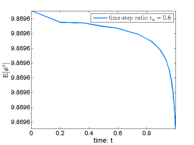
(a) Time-step ratio $r_{n}=0.8$

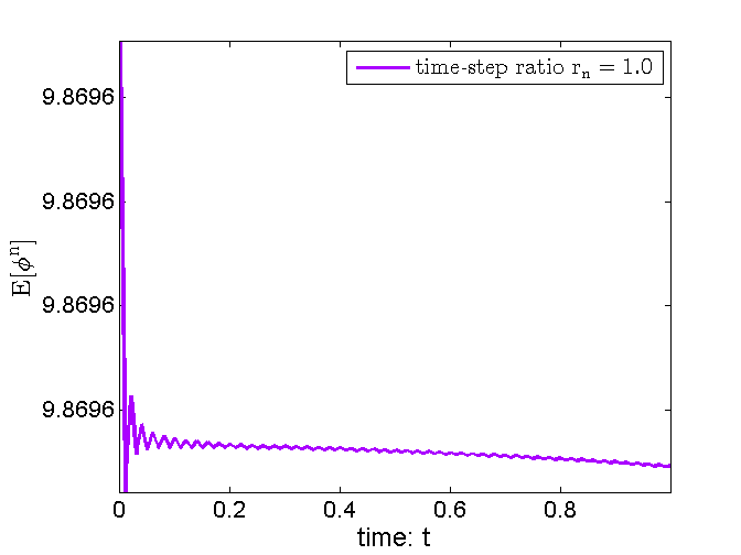
(b) Time-step ratio $r_{n}=1.0$

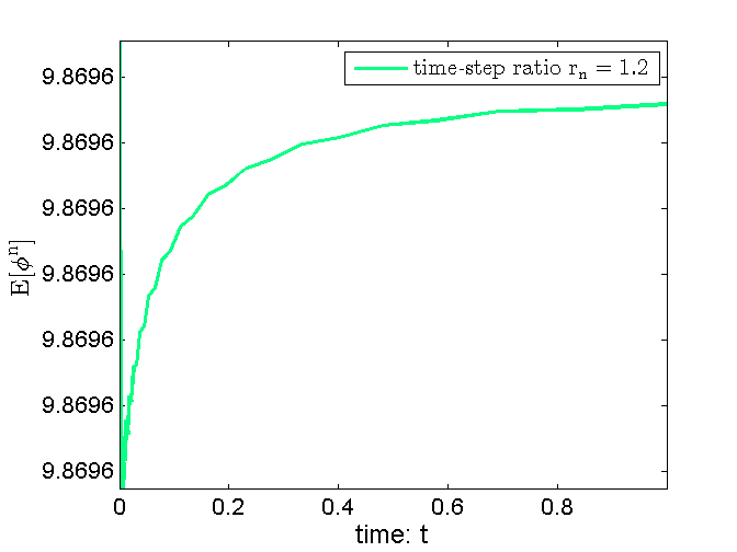
(c) Time-step ratio $r_{n}=1.2$

Figure 2: The original energy of the L1_a scheme (1.13) for different step ratios $r_{n}$.

At first, we test the discrete original energy $E\left[\phi^{n}\right]$ defined in (3.3) using the random initial data, although no discrete energy law for the L1_a scheme (1.13) is built theoretically. Figure 2 depicts the curves of original energy for the fractional order $\alpha=0.9$ on the time meshes generated by a fixed time-step ratio $r_{n}$ with $N=100$ until time $T=1$. As observed, the energy dissipation property is violated when the time-step ratios $r_{n}\geq 1$, so that the L1_a scheme (1.13) may be not suitable for practical simulation of the TFCH model. We thus focus on the numerical computations of the variable-step L1 scheme (1.11) and L1_h scheme (1.12) in what follows.

Table 11: CPU time and total time levels with different adaptive strategies.

  Time-stepping strategies L1 scheme L1_h scheme Total levels CPU (seconds) Total levels CPU (seconds) uniform step $\tau=5\times 10^{-3}$ 6030 240.526 6030 216.339 adaptive steps with $\eta=10$ 487 28.007 487 19.403 adaptive steps with $\eta=10^{2}$ 1092 51.448 1089 39.918 adaptive steps with $\eta=10^{3}$ 3178 133.169 3166 109.450  

We adopt the graded time meshes $t_{k}=T_{0}(k/N_{0})^{\gamma}$ together with the settings $\gamma=3,N_{0}=30$ and $T_{0}=0.01$ to resolve the weakly singularity for the THCH model. The treatment of remainder time interval is a great deal of flexibility such as the time-stepping strategy below [19, 25, 6],

$$\tau_{ada}=\max\Bigg{\{}\tau_{\min},\frac{\tau_{\max}}{\sqrt{1+\eta\big{\|}\partial_{\tau}\phi^{n}\big{\|}^{2}}}\Bigg{\}},$$ (4.10)

where $\eta>0$ is a user parameter, $\tau_{\max}=0.1$ and $\tau_{\min}=10^{-3}$ are the predetermined maximum and minimum time steps, respectively.

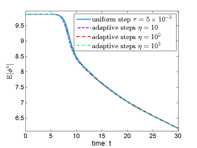
(a) Original energy $E\left[\phi^{n}\right]$

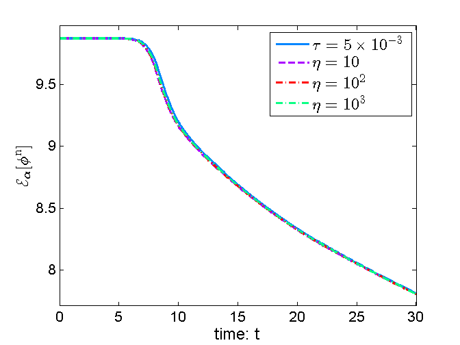
(b) Modified energy $\mathcal{E}_{\alpha}\left[\phi^{n}\right]$

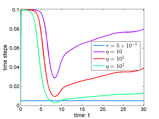
(c) Time steps $\tau_{n}$

Figure 3: Energy curves by uniform step and adaptive strategy with different parameters $\eta$.

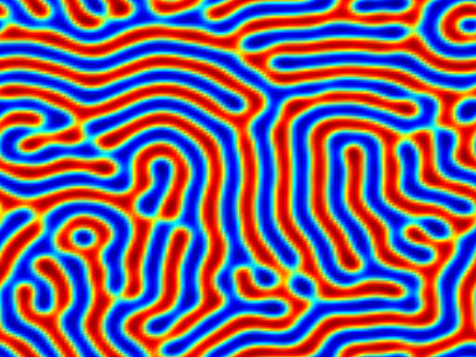
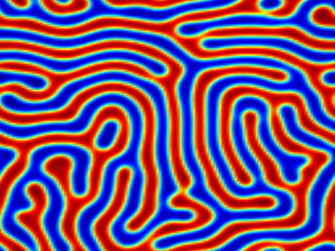
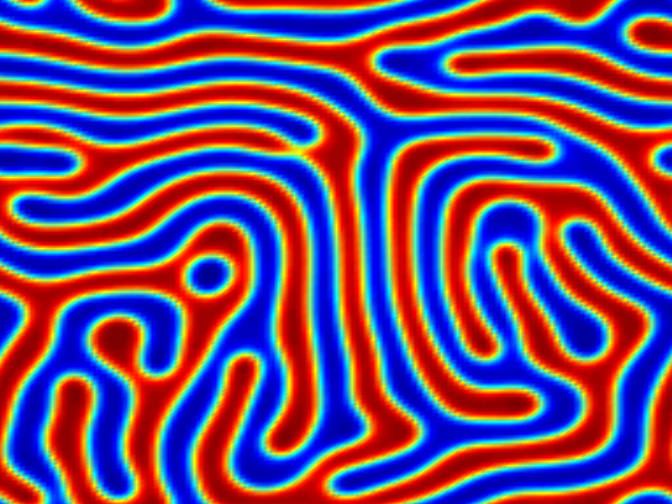
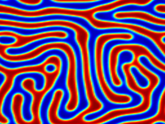
(a) The profile of $\phi$ with fractional order $\alpha=0.4$ at time $t=30,100,300,500.$

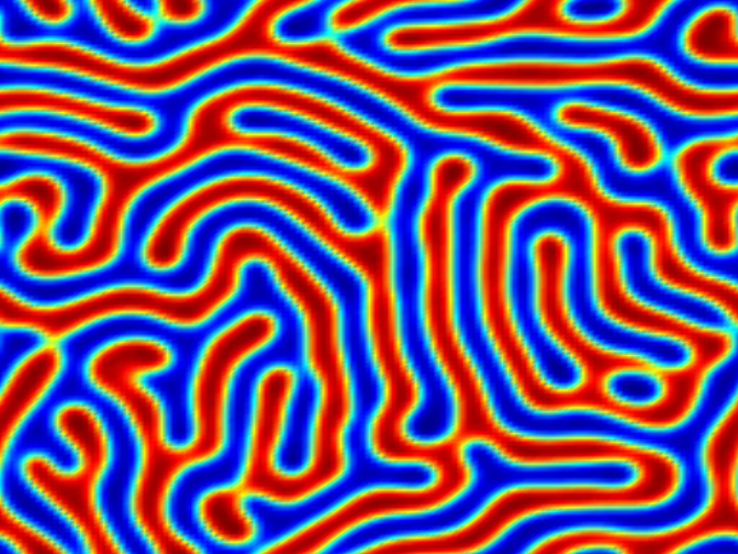
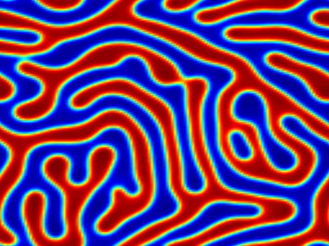
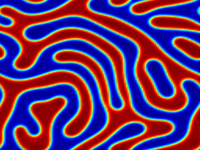
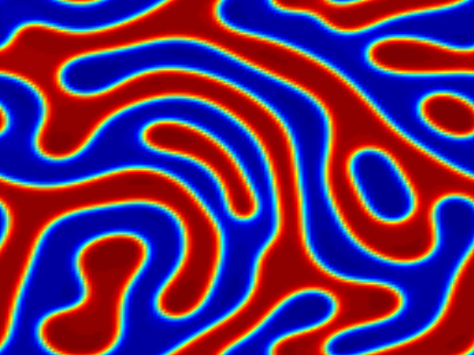
(b) The profile of $\phi$ with fractional order $\alpha=0.7$ at time $t=30,100,300,500.$

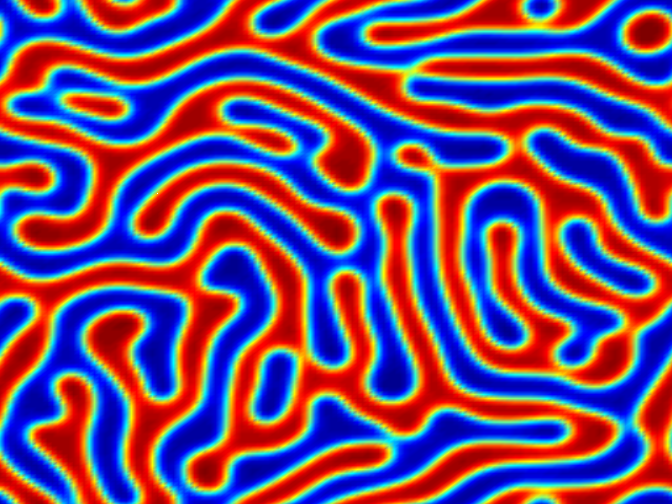
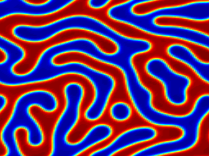
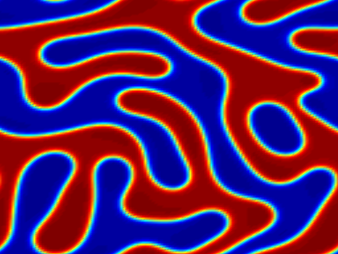
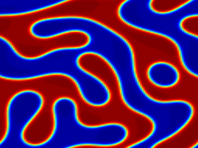
(c) The profile of $\phi$ with fractional order $\alpha=0.9$ at time $t=30,100,300,500.$

Figure 4: Snapshots of dynamic coarsening processes for different fractional orders $\alpha$.

To test the numerical performance of the adaptive time-stepping algorithm (4.10), we perform a comparative study by running the L1 scheme (1.11) and the L1_h scheme (1.12) on different time steps. We first apply a small uniform time step $\tau=5\times 10^{-3}$ to obtain the reference solution. Then we repeat the numerical simulation by using the adaptive time-stepping strategy with three different parameters $\eta=10,10^{2},10^{3}$, respectively.

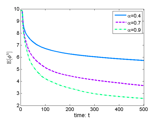
(a) Original energy $E\left[\phi^{n}\right]$

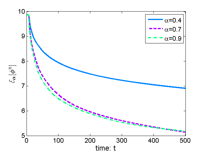
(b) Variational energy $\mathcal{E}_{\alpha}\left[\phi^{n}\right]$

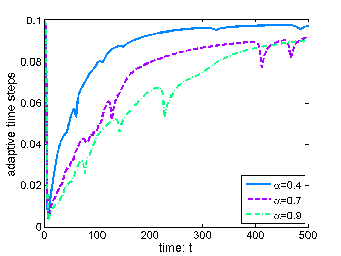
(c) Adaptive time steps $\tau_{n}$

Figure 5: Numerical results of the TFCH model with different fractional orders $\alpha$.

The numerical results are summarized in Figure 3. As can be seen, the numerical results using adaptive time-stepping are comparable to the reference solution. Also, one can observe that the adaptive time-steps are adjusted promptly by the parameters $\eta$: large (small) $\eta$ reinforces (reduces) the restriction to the time step sizes. The corresponding CPU time (in seconds) and the total time levels for different time-stepping strategies are listed in Table 11. The effectiveness of the adaptive time-stepping algorithm makes the long-time dynamics simulation practical. Note that, the numerical results of the L1_h scheme (1.12) are quite similar to those of the L1 scheme (1.11), and we thus omit them for brevity.

Finally, we perform the numerical simulation by using the adaptive time-stepping strategy (4.10) with the parameter $\eta=10^{3}$ until time $T=500$. The rest settings are kept the same as in the previous example. The profile of $\phi$ for the TFCH model (1.1) with different fractional orders $\alpha$ are depicted in Figure 4. They are consistent with the coarsening dynamics process reported in [16, 26]. The evolutions of the numerical energies and adaptive time steps during the coarsening dynamics are depicted in Figure 5. They suggest that the proposed variable-step methods effectively capture the multiple time scales in the long-time dynamical simulations.

References

- [1] M. Al-Maskari and S. Karaa. The time-fractional Cahn-Hilliard equation: analysis and approximation. IMA J. Numer. Anal., 2021. Doi:10.1093/imanum/drab025.
- [2] J. Cahn and J. Hilliard. Free energy of a nonuniform system I. interfacial free energy. J. Chem. Phys., 28:258–267, 1958.
- [3] L. Chen, J. Zhang, J. Zhao, W. Cao, H. Wang, and J. Zhang. An accurate and efficient algorithm for the time-fractional molecular beam epitaxy model with slope selection. Comput. Phys. Commun., 245:106842, 2019.
- [4] K. Cheng, C. Wang, and S. Wise. An energy stable BDF2 Fourier pseudo-spectral numerical scheme for the square phase field crystal equation. Comm. Comput. Phys., 26:1335–1364, 2019.
- [5] K. Cheng, C. Wang, S. Wise, and X. Yue. A second-order, weakly energy-stable pseudo-spectral scheme for the Cahn-Hilliard equation and its solution by the homogeneous linear iteration method. J. Sci. Comput., 69:1083–1114, 2016.
- [6] J. Huang, C. Yang, and Y. Wei. Parallel energy-stable solver for a coupled Allen–Cahn and Cahn–Hilliard system. SIAM J. Sci. Comput., 42:C294–C312, 2020.
- [7] B. Ji, H.-L. Liao, and L. Zhang. Simple maximum-principle preserving time-stepping methods for time-fractional Allen-Cahn equation. Adv. Comput. Math., 2020. doi:10.1007/s10444-020-09782-2.
- [8] S. Jiang, J. Zhang, Z. Qian, and Z. Zhang. Fast evaluation of the Caputo fractional derivative and its applications to fractional diffusion equations. Comm. Comput. Phys., 21:650–678, 2017.
- [9] N. Kopteva. Error analysis of the L1 method on graded and uniform meshes for a fractional-derivative problem in two and three dimensions. Math. Comput., 88:2135–2155, 2019.
- [10] S. Karaa. Positivity of discrete time-fractional operators with applications to phase-field equations. SIAM J. Numer. Anal., 59:2040–2053, 2021.
- [11] H.-L. Liao, D. Li, and J. Zhang. Sharp error estimate of nonuniform L1 formula for time-fractional reaction-subdiffusion equations. SIAM J. Numer. Anal., 56:1112–1133, 2018.
- [12] H.-L. Liao, T. Tang, and T. Zhou. Positive definiteness of real quadratic forms resulting from the variable-step approximation of convolution operators. arXiv:2011.13383v1, 2020.
- [13] H.-L. Liao, T. Tang, and T. Zhou. An energy stable and maximum bound preserving scheme with variable time steps for time fractional Allen-Cahn equation. SIAM J. Sci. Comput., 43:A3503–A3526, 2021.
- [14] H.-L. Liao, Y. Yan, and J. Zhang. Unconditional convergence of a fast two-level linearized algorithm for semilinear subdiffusion equations. J. Sci. Comput., 80:1–25, 2019.
- [15] H-L. Liao, X. Zhu, and J. Wang. An adaptive L1 time-stepping scheme preserving a compatible energy law for the time-fractional Allen-Cahn equation. Numer. Math. Theor. Meth. Appl., 2021. to appear. arXiv:2102.07577v1.
- [16] H. Liu, A. Cheng, H. Wang, and J. Zhao. Time-fractional Allen-Cahn and Cahn-Hilliard phase-field models and their numerical investigation. Comp. Math. Appl., 76:1876–1892, 2018.
- [17] J. López-Marcos. A difference scheme for a nonlinear partial integr-odifferential equation. SIAM J. Numer. Anal., 27:20–31, 1990.
- [18] I. Podlubny. Fractional differential equations. Academic Press, New York, 1999.
- [19] Z. Qiao, Z. Zheng, and T. Tang. An adaptive time-stepping strategy for the molecular beam epitaxy models. SIAM J. Sci. Comput., 22:1395–1414, 2011.
- [20] C. Quan, T. Tang, and J. Yang. How to define dissipation-preserving energy for time-fractional phase-field equations. CSIAM-AM, 1:478–490, 2020.
- [21] C. Quan, T. Tang, and J. Yang. Numerical energy dissipation for time-fractional phase-field equations. arXiv:2009.06178v1, 2020.
- [22] M. Stynes, E. O’Riordan, and J. L. Gracia. Error analysis of a finite difference method on graded meshes for a time-fractional diffusion equation. SIAM J. Numer. Anal., 55:1057–1079, 2017.
- [23] T. Tang, H. Yu, and T. Zhou. On energy dissipation theory and numerical stability for time-fractional phase field equations. SIAM J. Sci. Comput., 41:A3757–A3778, 2019.
- [24] J. Xu, Y. Li, S. Wu, and A. Bousquet. On the stability and accuracy of partially and fully implicit schemes for phase field modeling. Comput. Methods Appl. Mech. Eng., 345:826–853, 2019.
- [25] Z. Zhang and Z. Qiao. An adaptive time-stepping strategy for the Cahn-Hilliard equation. Comm. Comput. Phys., 11:1261–1278, 2012.
- [26] J. Zhao, L. Chen, and H. Wang. On power law scaling dynamics for time-fractional phase field models during coarsening. Comm. Non. Sci. Numer. Simu., 70:257–270, 2019.