PeleLM-FDF Large Eddy Simulator of Turbulent Combustion

Abstract

A new computational methodology, termed “PeleLM-FDF” is developed and utilized for high fidelity large eddy simulation (LES) of complex turbulent combustion systems. This methodology is constructed via a hybrid scheme combining the Eulerian PeleLM base flow solver with the Lagrangian Monte Carlo simulator of the filtered density function (FDF) for the subgrid scale reactive scalars. The resulting methodology is capable of simulating some of the most intricate physics of complex turbulence-combustion interactions. This is demonstrated by LES of a non-premixed CO/H₂ temporally evolving jet flame. The chemistry is modelled via a skeletal kinetics model, and the results are appraised via detail a posteriori comparisons against direct numerical simulation (DNS) data of the same flame. Excellent agreements are observed for the time evolution of various statistics of the thermo-chemical quantities, including the manifolds of the multi-scalar mixing. The new methodology is capable of capturing the complex phenomena of flame-extinction and re-ignition at a 1/512 of the computational cost of the DNS. The high fidelity and the computational affordability of the new PeleLM-FDF solver warrants its consideration for LES of practical turbulent combustion systems.

65C05, 65C30, 76F55, 76F80

1 Introduction

Since its original proof of concept [15, 38], the filtered density function (FDF) has become very popular for large eddy simulation (LES) of turbulent flows. This popularity is due to inherent capability of the FDF to account full statistics of the subgrid scale (SGS) quantities; and thus it is more accurate than conventional SGS models which are based on low order SGS moments. This superior performance comes at a price. The FDF transport equation is somewhat more difficult and computationally more expensive to solve, as compared to traditional LES schemes. The last decade has witnessed significant progress to improve FDF simulations, as evidenced by a rather large number of publications; e.g. Ref. [20, 88, 16, 13, 42, 44, 66, 70, 93, 6, 5, 3, 87, 59, 47, 48, 65, 37, 41, 46, 67, 53, 52, 51]. Parallel with these developments, there have also been extensive studies regarding the FDF accuracy & reliability [76, 39, 48, 14, 66], and sensitivity analysis of its simulated results [92, 91]. For comprehensive reviews of progress within the last decade, see Refs. [68, 85].

Despite the remarkable progress as noted, there is still a continuing demand for further improvements of LES-FDF for prediction of complex turbulent combustion systems. In particular, it is desirable to develop FDF tools which are of high fidelity, and are also computationally affordable. In this work, the PeleLM [50] base flow solver is combined with the parallel Monte Carlo FDF simulator [5, 4] in a hybrid manner that takes full advantage of modern developments in both strategies. PeleLM is a massively parallel simulator of reactive flows at low Mach numbers. These flows are of significant interest in several industries such as gas turbines, IC engines, furnaces and many others. The solver is based on block-structured AMR algorithm [9] through the AMReX numerical software library [89] (formerly called BoxLib [90]). This solver uses a variable density projection method [2, 57, 10] for solving three-dimensional Navier-Stokes and reaction-diffusion equations. The computational discretization is based on structured finite volume for spatial discretization, and a modified spectral deferred correction (SDC) algorithm [49, 55, 31, 23] for temporal integration. The solver is capable of dealing with complex geometries via the embedded boundary method [56, 21], and runs on modern platforms for parallel computing such as MPI + OpenMP for CPUs and MPI + CUDA or MPI + HIP for GPUs. The fidelity of PeleLM has been demonstrated to be effective for DNS of a variety of reactive turbulent flows [7, 18, 8, 17, 83]. Here, the PeleLM is augmented to include LES capabilities by hybridizing it with the FDF-SGS closure. The resulting solver is shown to be computationally efficient, and to produce results consistent with those generated by high-fidelity, and much more expensive DNS.

2 Formulation

We consider a variable density turbulent reacting flow involving $N_{s}$ species in which the flow velocity is much less than the speed of sound. In this flow, the primary transport variables are the fluid density $\rho(\mathbf{x},t)$, the velocity vector $u_{i}(\mathbf{x},t),\ i=1,2,3$ along the $x_{i}$ direction, the total specific enthalpy $h(\mathbf{x},t)$, the pressure $p(\mathbf{x},t)$, and the species mass fractions $Y_{\alpha}(\mathbf{x},t)\ (\alpha=1,2,\dots,N_{s})$. The conservation equations governing these variables are the continuity, momentum, enthalpy (energy) and species mass fraction equations, along with an equation of state [81]:

(1) $${\partial\rho\over\partial t}+{\partial\rho u_{i}\over\partial x_{i}}=0,$$

(2) $${\partial\rho u_{j}\over\partial t}+{\partial\rho u_{i}u_{j}\over\partial x_{i}}=-{\partial p\over\partial x_{j}}+{\partial\tau_{ij}\over\partial x_{i}},$$

(3) $${\partial\rho\phi_{\alpha}\over\partial t}+{\partial\rho u_{i}\phi_{\alpha}\over\partial x_{i}}=-{\partial J_{i}^{\alpha}\over\partial x_{i}}+\rho S_{\alpha},\ \ \ \alpha=1,2,\dots,\sigma=N_{s}+1,$$

(4) $$p=\rho R^{0}T\sum_{\alpha=1}^{N_{s}}Y_{\alpha}/{\cal M}_{\alpha},$$

where $t$ represents time, $R^{0}$ is the universal gas constant and ${\cal M}_{\alpha}$ denotes the molecular weight of species $\alpha$. Equation Eq. 3 represents transport of the species’ mass fractions and enthalpy in a common form with:

(5) $$\phi_{\alpha}\equiv Y_{\alpha},\ \alpha=1,2,\dots,N_{s},\ \ \phi_{\sigma}\equiv h=\sum_{\alpha=1}^{N_{s}}h_{\alpha}\phi_{\alpha}.$$

With the low Mach number approximation, the chemical source terms $S_{\alpha}$ are functions of the composition variables $\mbox{\boldmath$\phi$}=[Y_{1},Y_{2},\dots,Y_{N_{s}},h]$ only; i.e. $S_{\alpha}=S_{\alpha}(\mbox{\boldmath$\phi$})$. For a Newtonian fluid with zero bulk viscosity and Fickian diffusion, the viscous stress tensor $\tau_{ij}$ and the mass and the heat fluxes $J^{\alpha}_{i}\ (\alpha=1,2,\dots,\sigma$) are given by:

(6) $$\tau_{ij}=\mu\left({\partial u_{i}\over\partial x_{j}}+{\partial u_{j}\over\partial x_{i}}-{2\over 3}{\partial u_{k}\over\partial x_{k}}\delta_{ij}\right),\ \ \ J_{i}^{\alpha}=-\gamma{\partial\phi_{\alpha}\over\partial x_{i}},$$

where $\mu$ is the dynamic viscosity and $\gamma$ denotes the thermal and the mass molecular diffusivity coefficients. Both $\mu$ and $\gamma$ are assumed temperature dependent, and the molecular Lewis number is assumed to be unity.

Large eddy simulation involves the use of the spatial filtering operation [1]:

(7) $$\langle Q(\mbox{${\bf x}$},t)\rangle_{\ell}=\int_{-\infty}^{+\infty}Q(\mbox{${\bf x}$}^{\prime},t){\cal G}(\mbox{${\bf x}$}^{\prime},\mbox{${\bf x}$})d\mbox{${\bf x}$}^{\prime},$$

where ${\cal G}$ denotes the filter function of width $\Delta_{G}$, $\langle Q(\mbox{${\bf x}$},t)\rangle_{\ell}$ represents the filtered value of the transport variable $Q(\mbox{${\bf x}$},t)$. In variable density flows it is convenient to consider the Favre filtered quantity ${\langle Q(\mbox{${\bf x}$},t)\rangle_{L}=}{\langle\rho Q\rangle_{\ell}}/{\mbox{$\langle\rho\rangle_{\ell}$}}$. The application of the filtering operation to the transport equations yields:

(8) $${\partial\mbox{$\langle\rho\rangle_{\ell}$}\over\partial t}+{\partial\mbox{$\langle\rho\rangle_{\ell}$}\mbox{$\langle u_{i}\rangle_{L}$}\over\partial x_{i}}=0,$$

(9) $${\partial\mbox{$\langle\rho\rangle_{\ell}$}\mbox{$\langle u_{j}\rangle_{L}$}\over\partial t}+{\partial\mbox{$\langle\rho\rangle_{\ell}$}\mbox{$\langle u_{i}\rangle_{L}$}\mbox{$\langle u_{j}\rangle_{L}$}\over\partial x_{i}}=-{\partial\mbox{$\langle p\rangle_{\ell}$}\over\partial x_{j}}+{{\partial\langle\tau_{ij}\rangle_{\ell}}\over\partial x_{i}}-{\partial T_{ij}\over\partial x_{i}},$$

(10) $${\partial\mbox{$\langle\rho\rangle_{\ell}$}\mbox{$\langle\phi_{\alpha}\rangle_{L}$}\over\partial t}+{\partial\mbox{$\langle\rho\rangle_{\ell}$}\mbox{$\langle u_{i}\rangle_{L}$}\mbox{$\langle\phi_{\alpha}\rangle_{L}$}\over\partial x_{i}}=-{{\partial\langle J_{i}^{\alpha}\rangle_{\ell}}\over\partial x_{i}}-{\partial M^{\alpha}_{i}\over\partial x_{i}}+\langle\rho S_{\alpha}\rangle_{\ell},\ \ \ \alpha=1,2,\dots,\sigma,$$

where $T_{ij}=\mbox{$\langle\rho\rangle_{\ell}$}(\langle u_{i}u_{j}\rangle_{L}-\mbox{$\langle u_{i}\rangle_{L}$}\mbox{$\langle u_{j}\rangle_{L}$})$, and $\ M^{\alpha}_{i}=\mbox{$\langle\rho\rangle_{\ell}$}(\langle u_{i}\phi_{\alpha}\rangle_{L}-\mbox{$\langle u_{i}\rangle_{L}$}\mbox{$\langle\phi_{\alpha}\rangle_{L}$})$ denote the subgrid stress and the subgrid mass fluxes, respectively. The filtered reaction source terms are denoted by $\langle\rho S_{\alpha}\rangle_{\ell}=\mbox{$\langle\rho\rangle_{\ell}$}\mbox{$\langle S_{\alpha}\rangle_{L}$}\ (\alpha=1,2,\dots,N_{s})$.

3 Filtered Density Function

The complete SGS statistical information pertaining to the scalar field, is contained within the FDF, defined as [60]:

(11) $$F_{L}\left(\mbox{\boldmath$\psi$};\mbox{${\bf x}$},t\right)=\int^{+\infty}_{-\infty}\rho(\mbox{${\bf x}$}^{\prime},t)\zeta\left(\mbox{\boldmath$\psi$},\mbox{\boldmath$\phi$}(\mbox{${\bf x}$}^{\prime},t)\right)G(\mbox{${\bf x}$}^{\prime},\mbox{${\bf x}$})d\mbox{${\bf x}$}^{\prime},$$

where

(12) $$\zeta\left(\mbox{\boldmath$\psi$},\mbox{\boldmath$\phi$}(\mbox{${\bf x}$},t)\right)=\prod^{\sigma}_{\alpha=1}\delta\left(\psi_{\alpha}-\phi_{\alpha}(\mbox{${\bf x}$},t)\right).$$

In this equation, $\delta$ denotes the Dirac delta function and $\psi$ is the scalar array in the sample space. The term $\zeta$ is the “fine-grained” density [54]. With the condition of a positive filter kernel [80], $F_{L}$ has all of the properties of a mass density function [61]. Defining the “conditional filtered value” of the variable $Q(\mbox{${\bf x}$},t)$ as:

(13) $$\langle Q\mbox{$\Big{\arrowvert}$}\mbox{\boldmath$\psi$}\rangle_{\ell}\equiv\frac{\int^{+\infty}_{-\infty}Q\left(\mbox{${\bf x}$}^{\prime},t\right)\rho(\mbox{${\bf x}$}^{\prime},t)\zeta\left(\mbox{\boldmath$\psi$},\mbox{\boldmath$\phi$}(\mbox{${\bf x}$}^{\prime},t)\right)G\left(\mbox{${\bf x}$}^{\prime},\mbox{${\bf x}$}\right)d\mbox{${\bf x}$}^{\prime}}{F_{L}\left(\mbox{\boldmath$\psi$};\mbox{${\bf x}$},t\right)},$$

the FDF is governed by [4]:

$$\frac{\partial F_{L}}{\partial t}+\frac{\partial[\langle u_{i}(\mbox{${\bf x}$},t)|\mbox{\boldmath$\psi$}\rangle_{\ell}F_{L}]}{\partial x_{i}} =\frac{\partial}{\partial\psi_{\alpha}}\left[\left<\frac{1}{\rho(\mbox{\boldmath$\phi$})}\left.\frac{\partial J_{i}^{\alpha}}{\partial x_{i}}\right|\mbox{\boldmath$\psi$}\right>_{\ell}F_{L}\right]$$

(14) $$-\frac{\partial}{\partial\psi_{\alpha}}[S_{\alpha}(\mbox{\boldmath$\psi$})F_{L}].$$

This is the exact transport equation for the FDF, in which the effects of chemical reaction (the last term on the right hand side) appear in a closed form. The unclosed terms due to convection and molecular mixing are identified by the conditional averages (identified by a vertical bar). The gradient diffusion model, and the linear mean square estimation (LMSE) approximations are employed for closure of these terms. With these assumptions, the modelled transport equation for the FDF becomes [29]:

$$\frac{\partial F_{L}}{\partial t}+\frac{\partial[\mbox{$\langle u_{i}\rangle_{L}$}F_{L}]}{\partial x_{i}} =\frac{\partial}{\partial x_{i}}\left[(\gamma+\gamma_{t})\frac{\partial(F_{L}/\mbox{$\langle\rho\rangle_{\ell}$})}{\partial x_{i}}\right]$$

(15) $$+\frac{\partial}{\partial\psi_{\alpha}}\left[\Omega(\psi_{\alpha}-\langle\phi_{\alpha}\rangle_{L})F_{L}\right]-\frac{\partial}{\partial\psi_{\alpha}}\left[S_{\alpha}\left(\mbox{\boldmath$\psi$}\right)F_{L}\right],$$

where $\gamma_{t}$ is the turbulent viscosity model [79], $\Omega=C_{\phi}\left(\gamma+\gamma_{t}\right)/\left(\langle\rho\rangle_{\ell}\Delta_{G}^{2}\right)$ is the SGS mixing frequency [61, 54], and $C_{\phi}$ is a model constant.

4 Hybrid PeleLM-FDF Solver

Equation Eq. 15 may be integrated to obtain the modeled transport equations for the SGS moments, e.g. the filtered mean, $\langle\phi_{k}\rangle_{L}$ and the SGS variance $\mbox{${\tau}$}_{k}\equiv\langle\phi_{k}^{2}\rangle_{L}-\langle\phi_{k}\rangle^{2}_{L}$. A convenient means of solving this equation is via the Lagrangian Monte Carlo (MC) procedure [85]. In this procedure, each of the MC elements (particles) undergo motion in physical space by convection due to the filtered mean flow velocity and diffusion due to molecular and subgrid diffusivities. These are determined by viewing Eq. Eq. 15 as a Fokker-Planck equation, for which the corresponding Langevin equations describing transport of the MC particles are [64, 24]:

(16) $$dX_{i}(t)=\left[\mbox{$\langle u_{i}\rangle_{L}$}+\frac{1}{\mbox{$\langle\rho\rangle_{\ell}$}}\frac{\partial(\gamma+\gamma_{t})}{\partial x_{i}}\right]dt+\sqrt{2(\gamma+\gamma_{t})/\mbox{$\langle\rho\rangle_{\ell}$}}\ dW_{i}(t),$$

with the change in the compositional makeup according to:

(17) $$\frac{d\phi_{k}^{+}}{dt}=-\Omega\left(\phi_{k}^{+}-\langle\phi_{k}\rangle_{L}\right)+S_{k}\left(\mbox{\boldmath$\phi$}^{+}\right)\;\left(k=1,2,\dots N_{s}+1\right).$$

In these equations, ${W}_{i}$ denotes the Wiener-Levy process, $\phi_{k}^{+}=\phi_{k}\left(\mathbf{X},t\right)$ is the scalar value of the particle with the Lagrangian position $X_{i}$.

AMReX library is a very powerful computational software with many useful functions, templates and classes including linear solvers [82] and particle containers [45]. The latter one, is especially useful for our purpose. The principal algorithm is based on a variable density projection method for low Mach number flows is described in Ref. [19]. The domain is discretized by an ensemble of finite-volume cells and the particles are free move within the domain (Fig. 1). The MC procedure is implemented by deriving a new class from the particle container of the AMReX library, adding all the required functions. The particle transport as given by the SDEs Eq. 16 is tracked via Euler-Maruyama method [40], The compositional makeup (Eq. Eq. 17) is implemented with variety of methods involving third-party solvers like VODE [12], CVODE [36], and our in-house adaptive Runge-Kutta solver.

With the hybrid scheme as developed, some of the quantities are obtained by MC-FDF, some by the base flow solver (PeleLM) and some by both. So, there is a “redundancy” in determination of some of the quantities. In general, all of the equations for the filtered quantities can be solved by PeleLM, in which all of the unclosed terms are evaluated by the MC-FDF solver. This process can be done at any filtered SGS moment level [3]. With the hydrodynamic solver given by PeleLM, the scalar transport is implemented via both of these ways. In doing so, the filtered source terms are evaluated by the ensemble values over the MC particles:

(18) $$\langle S_{\alpha}\left(\mbox{${\bf x}$},t\right)\rangle_{L}\approx\frac{1}{N_{E}}\sum_{n\in\Delta_{E}}S_{\alpha}(\mbox{\boldmath$\phi$}^{(n)}),$$

where $N_{E}$ is number of particles within the $\Delta_{E}$ neighborhood of point ${\bf x}$. The choice of $\Delta_{E}$ is independent of the grid size $\Delta x$, and the LES filter size $\Delta_{G}$. It is desirable to set $\Delta_{E}$ as small as possible. The particle-grid interaction is schematically illustrated in Fig. 1(a), while the example of an actual hybrid Eulerian-Lagrangian simulation is shown in Fig. 1(b). The transfer of information from the grid points to the MC particles is accomplished via a linear interpolation.

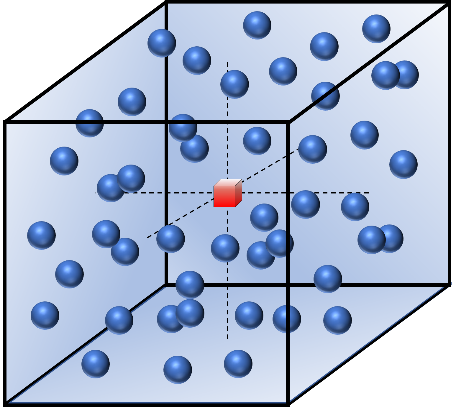
(a)

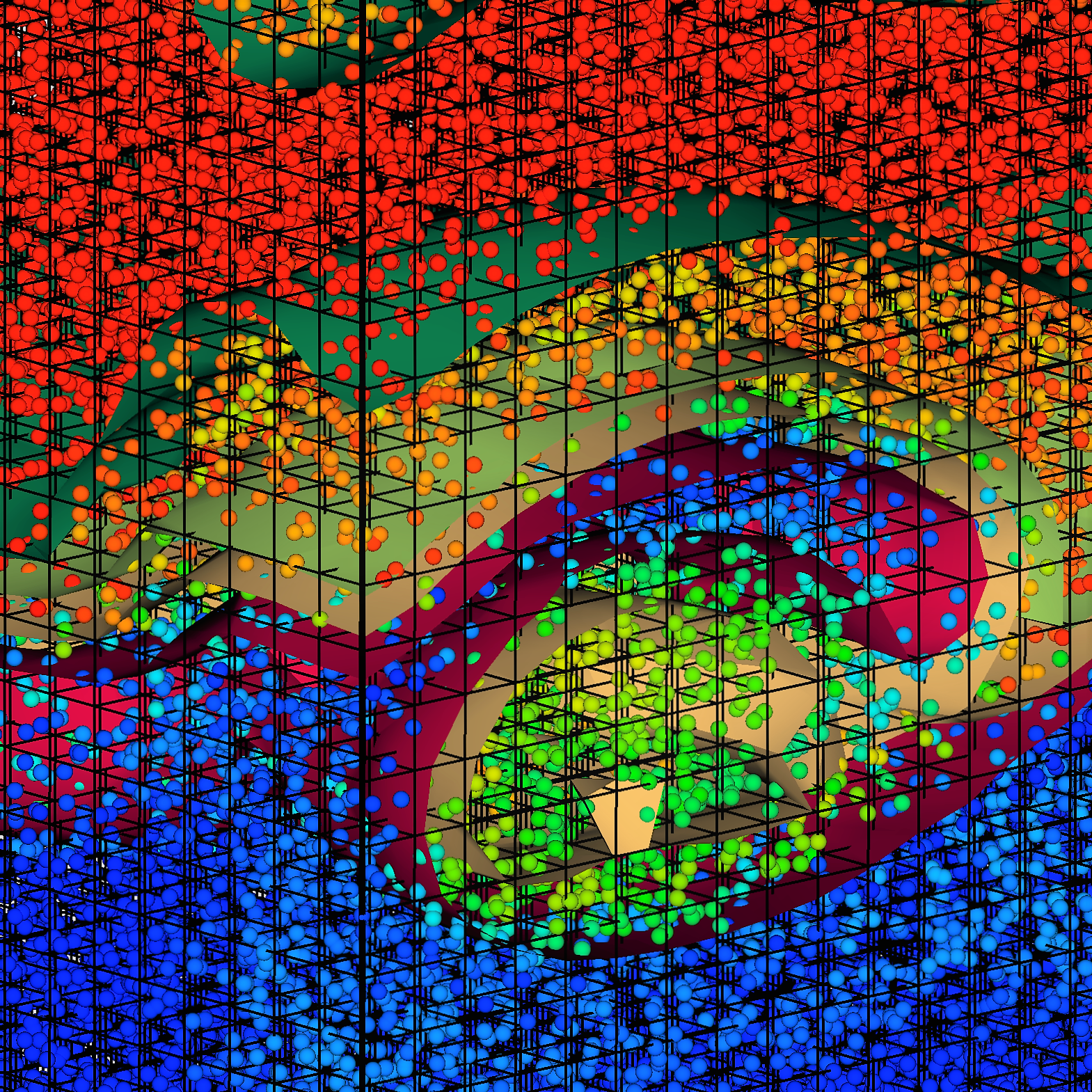
(b)

Figure 1: (a) Ensemble averaging in MC simulations. The red cube denotes the finite volume cell center, and the blue spheres denote the MC particles. (b) Example of MC particles within the Eulerian field identified by PeleLM. The colors of the MC particles provide a measure of the particle’s scalar values.

5 Flow Configuration and Model Specifications

The performance of the PeleLM-FDF solver is assessed by conducting LES of a temporally evolving planar turbulent CO/H₂ jet flame. This flame has been the subject of detailed DNS [33], and several subsequent modeling and simulations [86, 63, 78, 84, 69]. The flame is rich with strong flame–turbulence interactions resulting in local extinction followed by re-ignition. The flow configuration is the same as that considered in DNS and is depicted in Fig. 2. The jet consists of a central fuel stream of width $H$ surrounded by counter-flowing oxidizer streams. The fuel stream is comprised of 50$\%$ of CO, 10$\%$ H₂ and 40$\%$ N₂ by volume, while oxidizer streams contain 75$\%$ N₂ and 25$\%$ O₂. The initial temperature of both streams is 500K and thermodynamic pressure is set to 1 atm. The velocity difference between the two streams is $U=276$m/s. The fuel stream velocity and the oxidiser stream velocity are $U/2$ and $-U/2$, respectively. The Reynolds number, based on $U$ and $H$ is $Re=9,079$. The sound speeds in the fuel and oxidizer streams denoted as $C_{1}$ and $C_{2}$, respectively and the Mach number $Ma=U/\left(C_{1}+C_{2}\right)=0.3$ is small enough to justify a low Mach number approximation. The combustion chemistry is modelled via the skeletal kinetics, containing 11 species with 21 reaction steps [33]. The initial conditions are taken directly from DNS. The boundary conditions are periodic in stream wise ($x$) and spanwise ($z$) directions, and the outflow boundary conditions imposed at $y=\pm L_{y}/2$. The models in FDF are the same as those in previous LES-FDF [4], with minor upgrades. The SGS stresses and mass fluxes are modeled by the standard Boussinesq approximation [75, 25], and the gradient diffusion approximation, respectively. The SGS viscosity coefficient $\mu_{t}$ is calculated using the Vreman’s model [79]. The model parameters are: $C_{\phi}=5$, $c=0.05625$ and $Sc_{t}=Pr_{t}=0.7$.

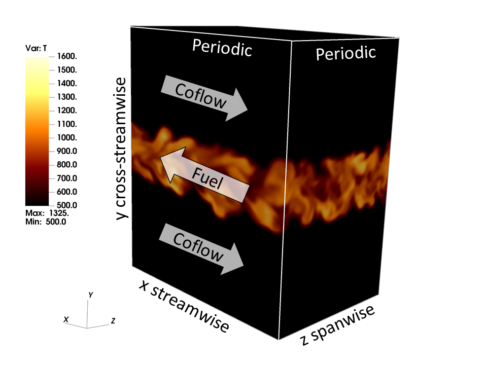
Figure 2: Schematics of the temporally developing turbulent jet flame. The jet consists of a central fuel stream surrounded by two counter-flowing oxidizer streams. The fuel stream is comprised of 50$\%$ of CO, 10$\%$ H₂ and 40$\%$ N₂ by volume, while oxidizer streams contain 75$\%$ N₂ and 25$\%$ O₂. The initial temperature of both streams is 500K and the thermodynamic pressure is set to 1 atm.

The size of the computational domain is $L_{x}\times L_{y}\times L_{z}=12H\times 14H\times 8H$. The time is normalized by $t_{j}=H/U$. The domain is discretized into equally spaced structured fixed grids of size $N_{x}\times N_{y}\times N_{z}=108\times 126\times 72$. The resolution, as selected, is the largest that was conveniently available to us, and kept the SGS energy within the allowable $15\%\sim 20\%$ of the total energy. This resolution should be compared with $N_{x,DNS}\times N_{y,DNS}\times N_{z,DNS}=864\times 1008\times 576$ grids as utilized in DNS [33]. The sizes of the ensemble domain, the subgrid filter and the finite-volume cell are taken to be equal $\Delta_{E}=\Delta_{G}=\Delta x=\Delta y=\Delta z=L_{x}/N_{x}$, and the timestep for temporal integration is $\Delta t=10^{-7}s$. The number of MC particles per grid point is set to 64; so there are over 62.7 million MC particles portraying the FDF at all time. With a factor of 512 times smaller number of grids, the total computational time for the simulations is around 400 CPU hours on 2 nodes of 28-core Intel Xeon E5-2690 2.60 GHz (Broadwell) totalling 56 processors.

The simulated results are analyzed both instantaneously and statistically. In the former, the instantaneous contours (snap-shots) and the scatter plots of the reactive scalar fields are considered. This pertains to the temperature and mass fractions of all of the species. In the latter, the “Reynolds-averaged” statistics are constructed. With the assumption of a temporally developing layer, the flow is homogeneous in the $z-$ and the $x-$ directions. Therefore, all of the Reynolds averaged values, denoted by an overline, are temporally evolving and determined by ensemble averaging over the $x-z$ planes. The resolved stresses are denoted by $R\left(a,b\right)=\overline{\langle a\rangle_{L}\langle b\rangle_{L}}-\left(\overline{\langle a\rangle_{L}}\right)\left(\overline{\langle b\rangle_{L}}\right)$, and the total stresses are denoted by $r\left(a,b\right)=\overline{\left(ab\right)}-\overline{a}\overline{b}$. The latter can be evaluated directly from the fine-grid DNS data $r_{\text{DNS}}\left(a,b\right)$. In LES with the assumption of a generic filter, i.e. $\overline{\langle Q\rangle_{L}}=\overline{Q}$, the total stresses are approximated by $r_{\text{LES}}\left(a,b\right)=R\left(a,b\right)+\overline{\tau\left(a,b\right)}$ [26, 77]. The root mean square (RMS) values are square roots of these stresses. To analyze the compositional flame structure, the “mixture fraction” field $Z(\mbox{${\bf x}$},t)$ is also constructed. Bilger’s formulation [11, 58] is employed for this purpose.

6 Presentation of Results

For the purpose of flow visualization, the contour plots of the temperate field are presented in Fig. 3 for several consecutive time-instances. These contours show the formation of structures within the flow, and the growth of the layer from the initial laminar to a highly three-dimensional turbulent flow. To demonstrate the consistency, comparisons are made between the filtered values as obtained by the Lagrangian and Eulerian simulators. Fig. 4 shows the instantaneous scatter plots of the temperature and mixture fraction, and Fig. 5 shows the Reynolds averaged values of these variables. The similarity of FDF and PeleLM results is evident.

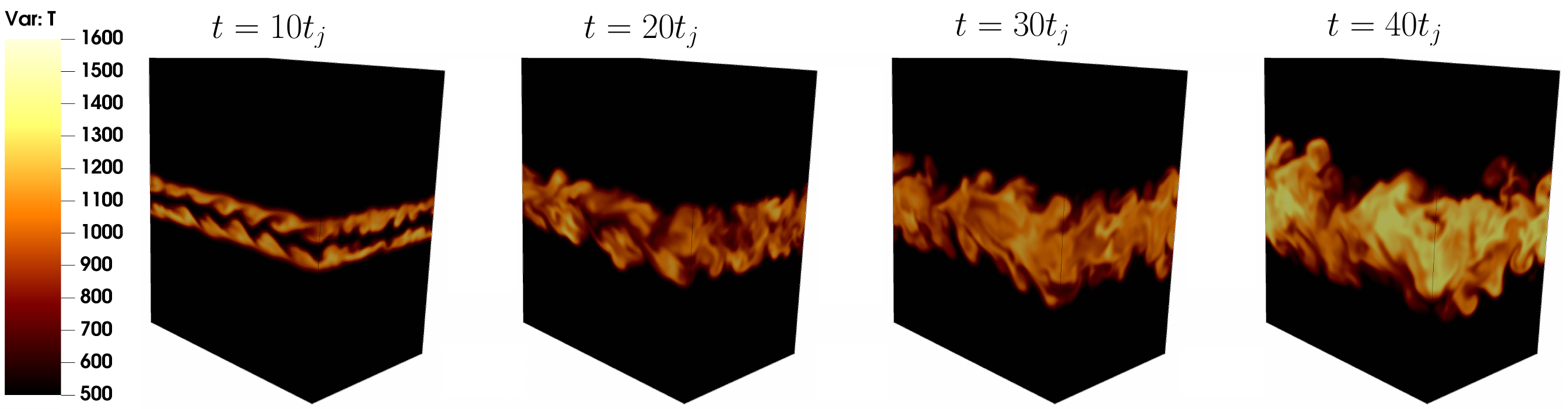
Figure 3: Temporal evolution of the temperature field.

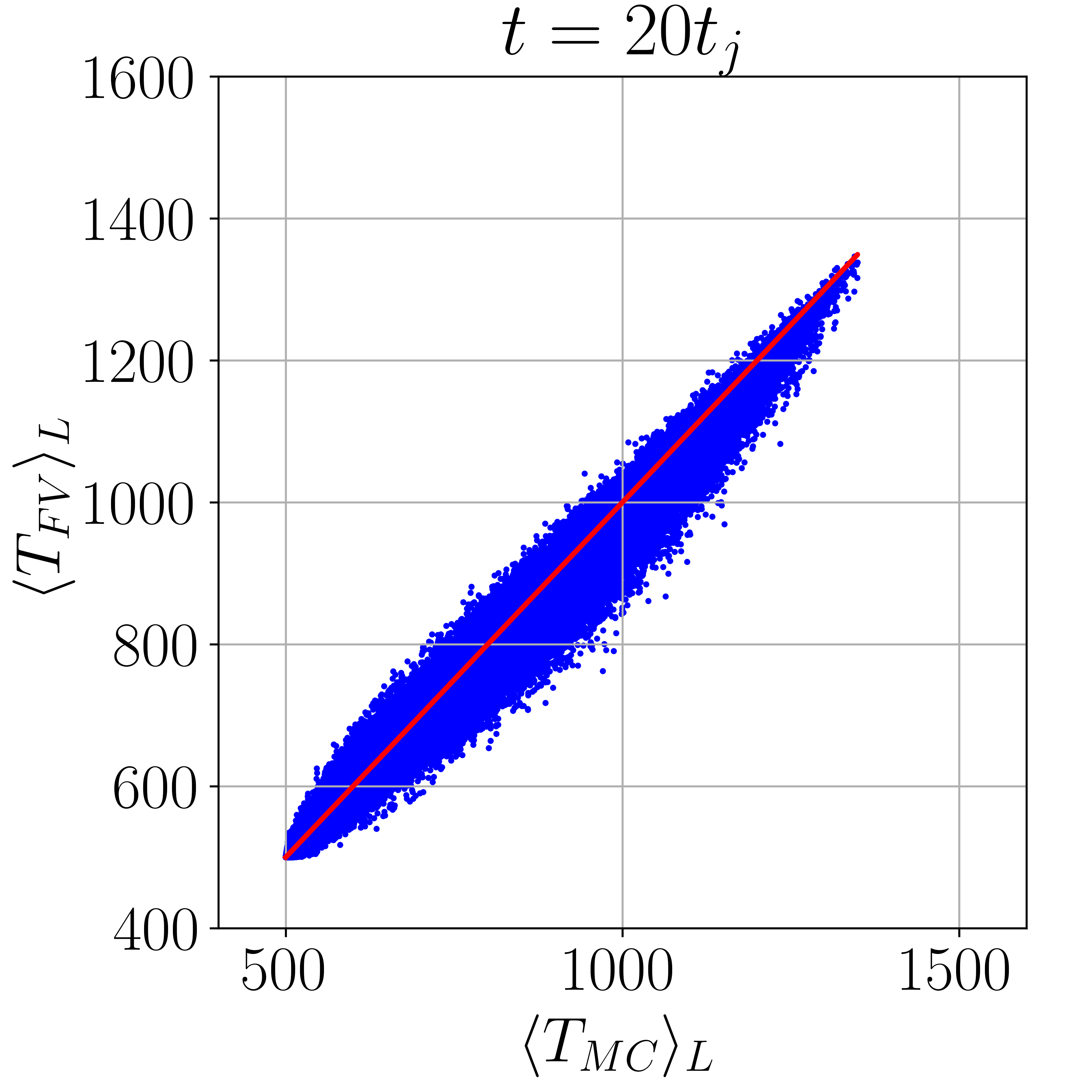
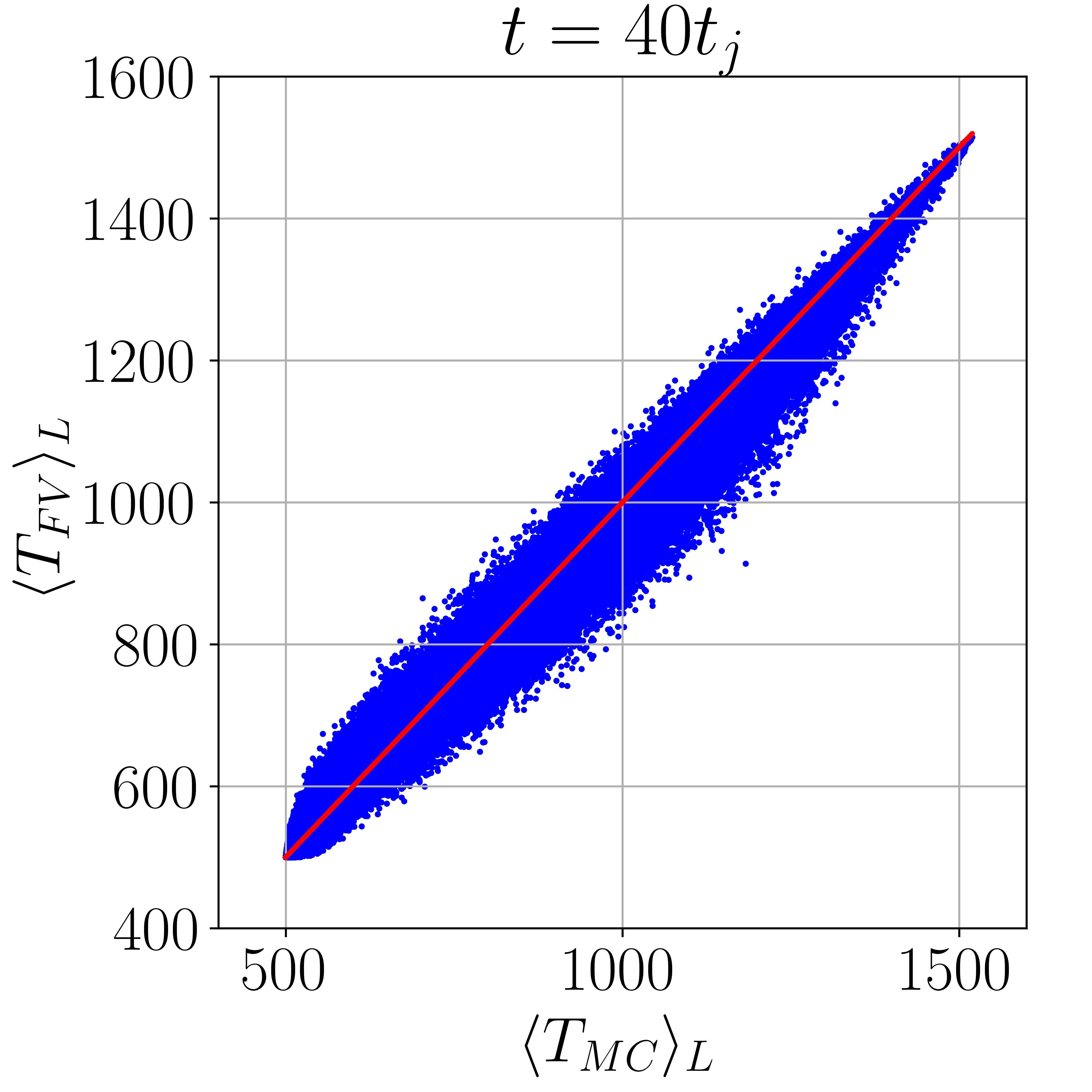
(a) Temperature

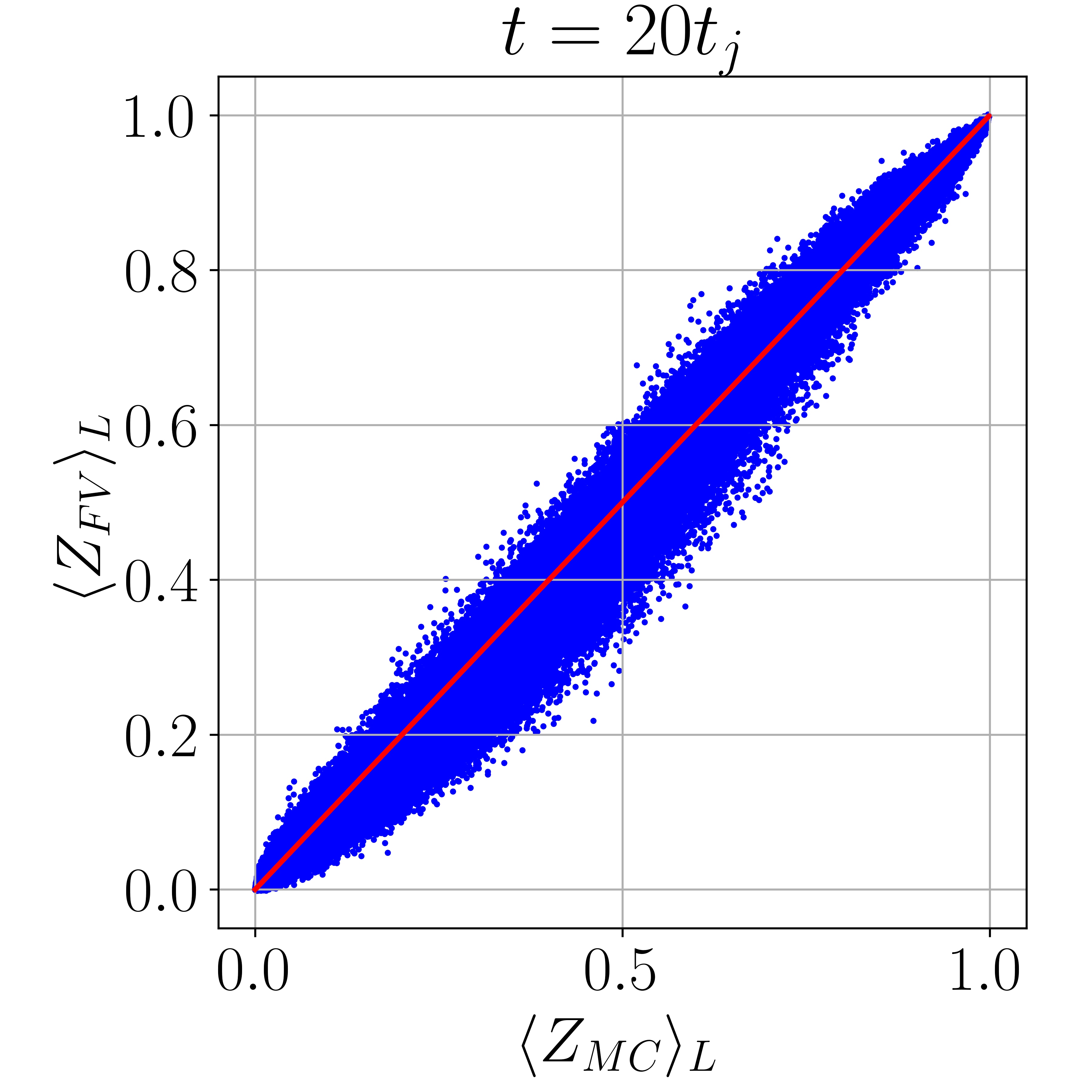
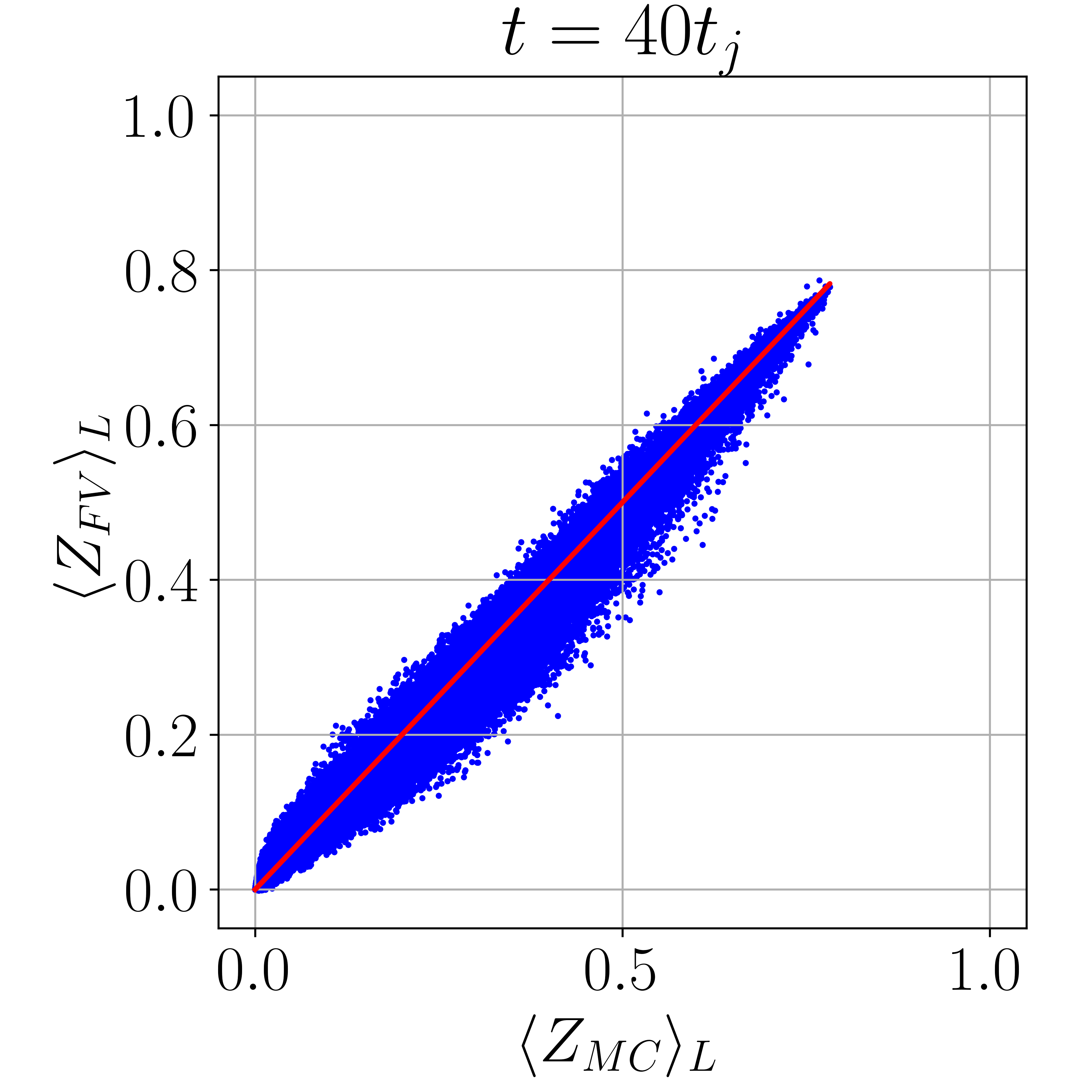
(b) Mixture fraction

Figure 4: Scatter plots of the Eulerian vs. the Lagrangian filtered values.

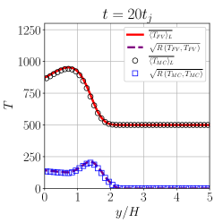
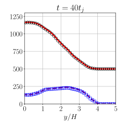
(a) Temperature

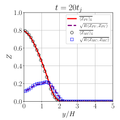
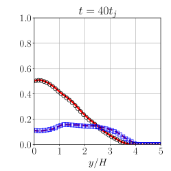
(b) Mixture fraction

Figure 5: Reynolds-averaged Eulerian (lines) vs. the Lagrangian filtered (symbols) values in the cross-stream direction.

The fidelity of LES predictions are assessed via comparisons with DNS. This is shown for the first and second Reynolds-moments of the mixture fraction, the temperature. and mass fractions of major species (CO, CO₂) at several time levels in Fig. 6. Additionally, 2D slice plots of LES-FDF and DNS are shown in Fig. 7 for more detailed view. In all of these cases, the DNS captures more of the small scale features which are filtered out by LES. Therefore, the spreading rate as predicted by LES is somewhat larger than that in DNS. The initial decrease of the temperature at $t\approx 20t_{j}$ is an indication of flame extinction, and its increase at later times $(t\approx 40t_{j})$ signals re-ignition.

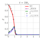
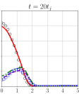
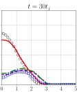
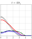
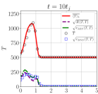
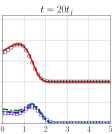
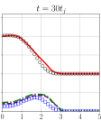
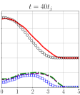
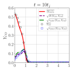
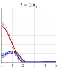
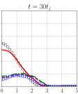
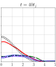
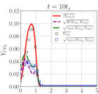
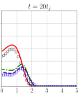
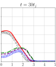
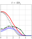
Figure 6: Reynolds-averaged mean and RMS values of the mixture fraction ($Z$), temperature ($T$), CO mass fraction ($Y_{CO}$), and CO₂ mass fraction ($Y_{CO_{2}}$). Lines and symbols denote LES and DNS results, respectively.

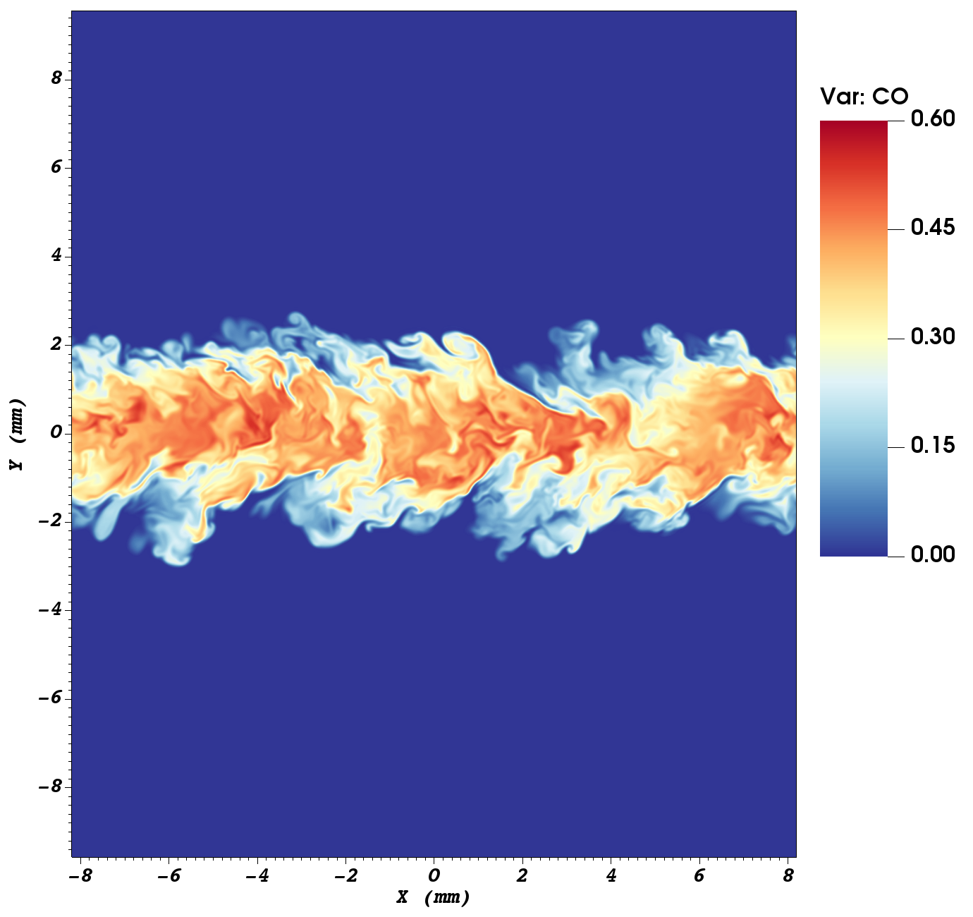
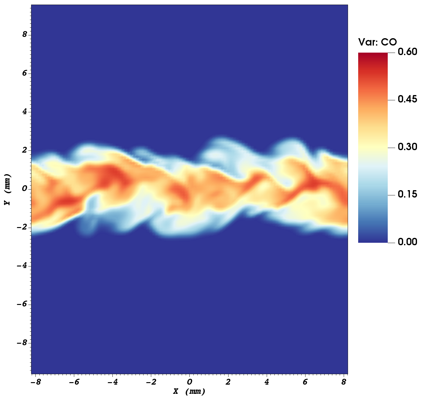
(a) $t=20t_{j}$

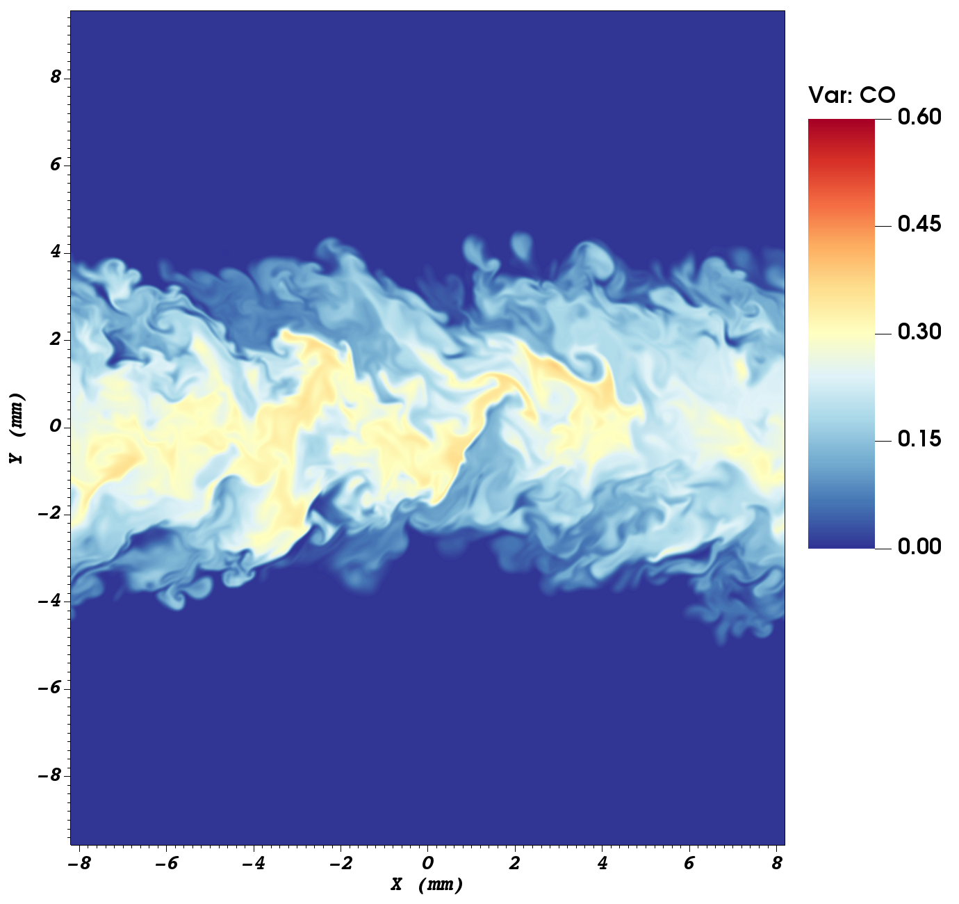
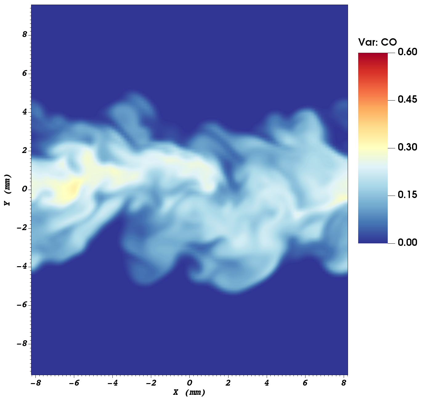
(b) $t=40t_{j}$

Figure 7: Instantaneous slice plots at $z=0$ of CO mass fraction obtained from DNS (left) and LES-FDF (right).

As an evidence of overall layer growth, the mixture fraction thickness is constructed. This thickness in defined as $\delta_{Z}=2\ {\rm arg\ min}\left(\left|\overline{Z}\left(y\right)-\epsilon\right|\right)$ for $y>0$, where $\epsilon$ is small positive number. The temporal evolution of this thickness is shown in Fig. 8, and indicates that the growth of a turbulent layer predicted by LES is close to that obtained by DNS at initial times. However, as the flow develops the LES predicts a larger spreading of the layer.

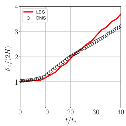
Figure 8: Temporal evolution of mixture fraction thickness. Lines and symbols denote the LES and DNS values, respectively.

The flame extinction phenomenon and its subsequent re-ignition is explained in terms of the dissipation of the mixture fraction: $\chi=2\gamma/\rho\nabla Z\cdot\nabla Z$ [58, 30]. The Reynolds-averaged values of this dissipation, implicitly modelled here as: $\langle\chi\rangle_{L}=2\Omega\tau\left(Z,Z\right)$ are shown in Fig. 9. All of the predicted results agree very well with DNS measured data. At initial times, when the dissipation rates are large, the flame cannot be sustained and is locally extinguished. At later times, when the dissipation values are lowered, the flame is re-ignired and the temperature increases. This dynamic is more clearly depicted in Fig. 10, where the expected temperature values conditioned on the mixture fraction are shown. By $t=20t_{j}$ the temperature at the stoichimetric mixture fraction ($Z_{st}=0.42$) decreases from $T=1400K$, stays below extinction limit for a while, and then rises after $t=30t_{j}$. The agreement with DNS data for this conditional expected value is very good.

To provide a more quantitative assessment of the flame structure within the entire domain, an “extinction marker” is defined: $M_{ext}=\left(H\left(Y_{OH}-Y_{OH,c}\right)|Z=Z_{st}\right)$ [32]. Here $Y_{OH,c}=0.0007$ is a cut-off mass fraction of hydroxyl radical and $H\left(x\right)$ denotes the Heaviside function. The choice of OH mass fraction as a main scalar used in marker is made upon a visual inspection of the fields of heat release. (A video-clip is provided in Supplementary Materials.) The volume averaged extinction marker defines the probability of a point experiencing extinction$\frac{1}{V}\int_{V}M_{ext}dV=P\left(Z=Z_{st},Y_{OH}\leq Y_{OH,c}\right)$ and its evolution over time is shown in Fig. 11(a). The excellent agreement between LES and DNS on the figure indicates that the timings of extinction and re-ignition as predicted by LES are accurate. The temporal evolution of the expected temperature conditioned on the stoichiometric mixture fraction in Fig. 11(b) corroborates the onset of extinction due to high dissipation and the subsequent re-ignitionl at low dissipation. The increase of temperature at final times is accompanied by $Y_{CO2}$ production and $Y_{CO}$ consumption at later times, as observed in Fig. 6.

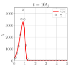
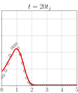
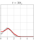
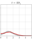
Figure 9: Reynolds-averaged values of scalar dissipation rate. Lines and symbols denote the LES and DNS values, respectively.

A more comprehensive comparison with DNS is done by examination of the mixture fraction PDFs in Fig. 12. In DNS these PDF generated by sampling of $N_{x,DNS}\times 8\times N_{z,DNS}$ near the center-plane ($\left|y\right|<\Delta y$) of the jet (8 cross-stream planes)). The LES generated PDFs are based on sampling of $N_{x}\times 2\times N_{z}$ (2 cross-stream planes). While the two sets of PDFs are qualitatively the same, there are some small quantitative differences. The DNS generated PDFs tend to be concentrated near the higher mixture fraction values. This is consistent with the observations made in Fig. 6, indicating a higher jet spreading rate in LES. However, the width of the PDFs are the same, consistent with the RMS values shown in Fig. 6. To portray the dynamics of multi-scalar mixing and reaction, the joint PDFs of the scalar variables must be considered. The mixture fraction and the mass fraction of the CO₂ are considered, and the results are shown in Fig. 13. In both cases, as the flow becomes fully turbulent at $t=40t_{j}$, the PDFs tend to have a multi-variate Gaussian distribution. In all cases, the LES predicted PDFs are in excellent agreement with those depicted by DNS. Finally, to asses the LES predictions of the overall compositional structure, three-dimensional scatter plots of the mixture fraction, the mass fraction of oxidant O₂ and the mass fraction of hydroxyl radical OH colored by temperature are shown in Fig. 14. Again, the manifolds as predicted by LES-FDF are in very good agreements with those depicted by DNS.

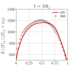
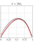
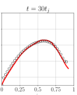
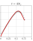
Figure 10: Volume averaged temperature conditioned on mixture fraction. Lines and symbols denote the LES and DNS values, respectively

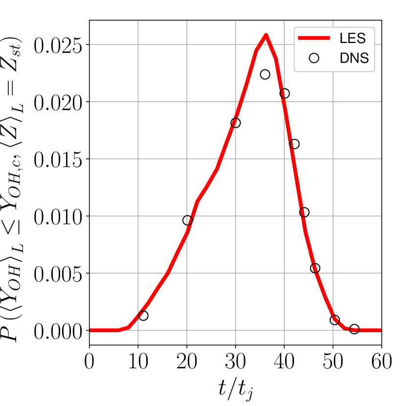
(a) Volume averaged extinction marker

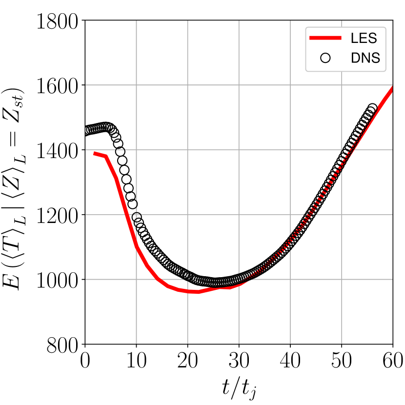
(b) Mean temperature on the stoichiometric surface

Figure 11: Temporal evolution of average extinction and re-ignition. Lines and symbols denote the LES and DNS values, respectively.

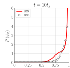
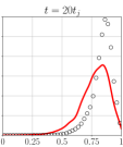
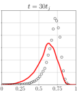
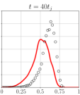
Figure 12: Probability density function of mixture fraction about $y=0$ plane. Lines and symbols denote the LES and DNS values, respectively.

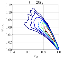
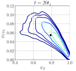
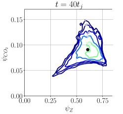
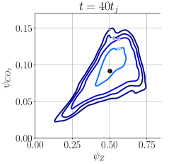
Figure 13: Joint probability density functions of mixture fraction and $Y_{CO_{2}}$ about $y=0$ plane of DNS (left) and LES (right).

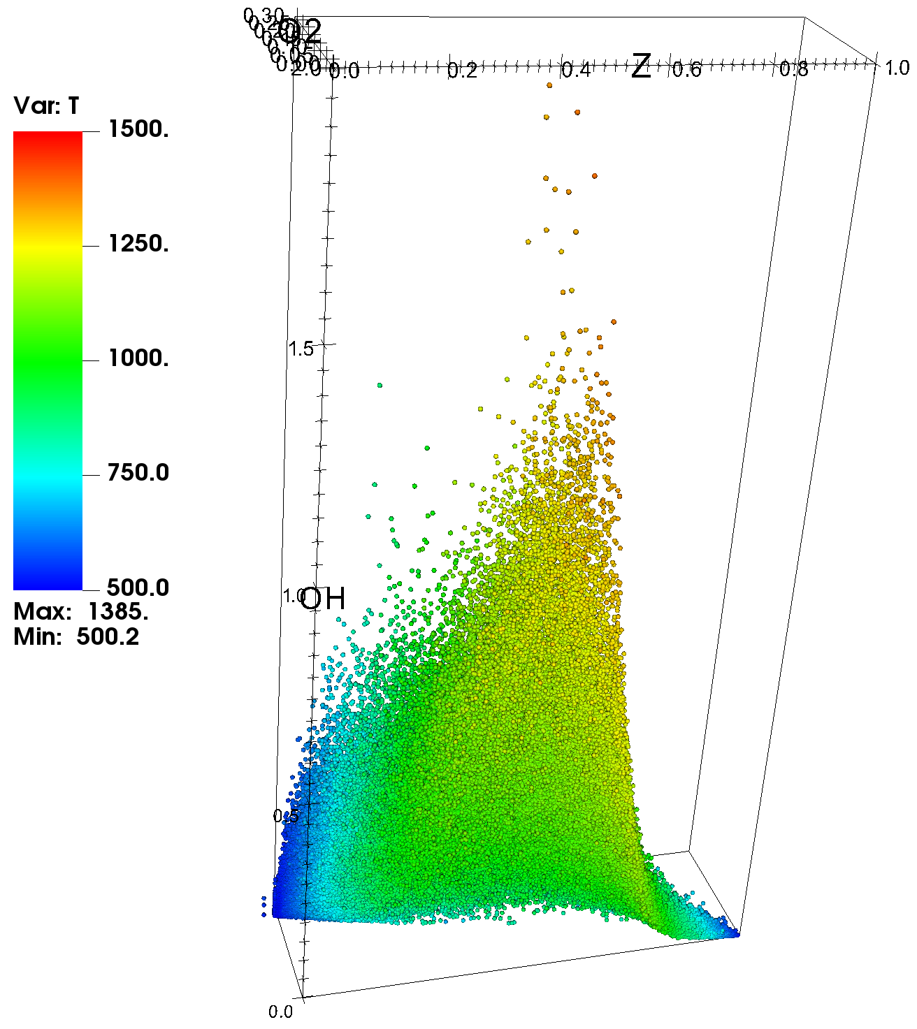
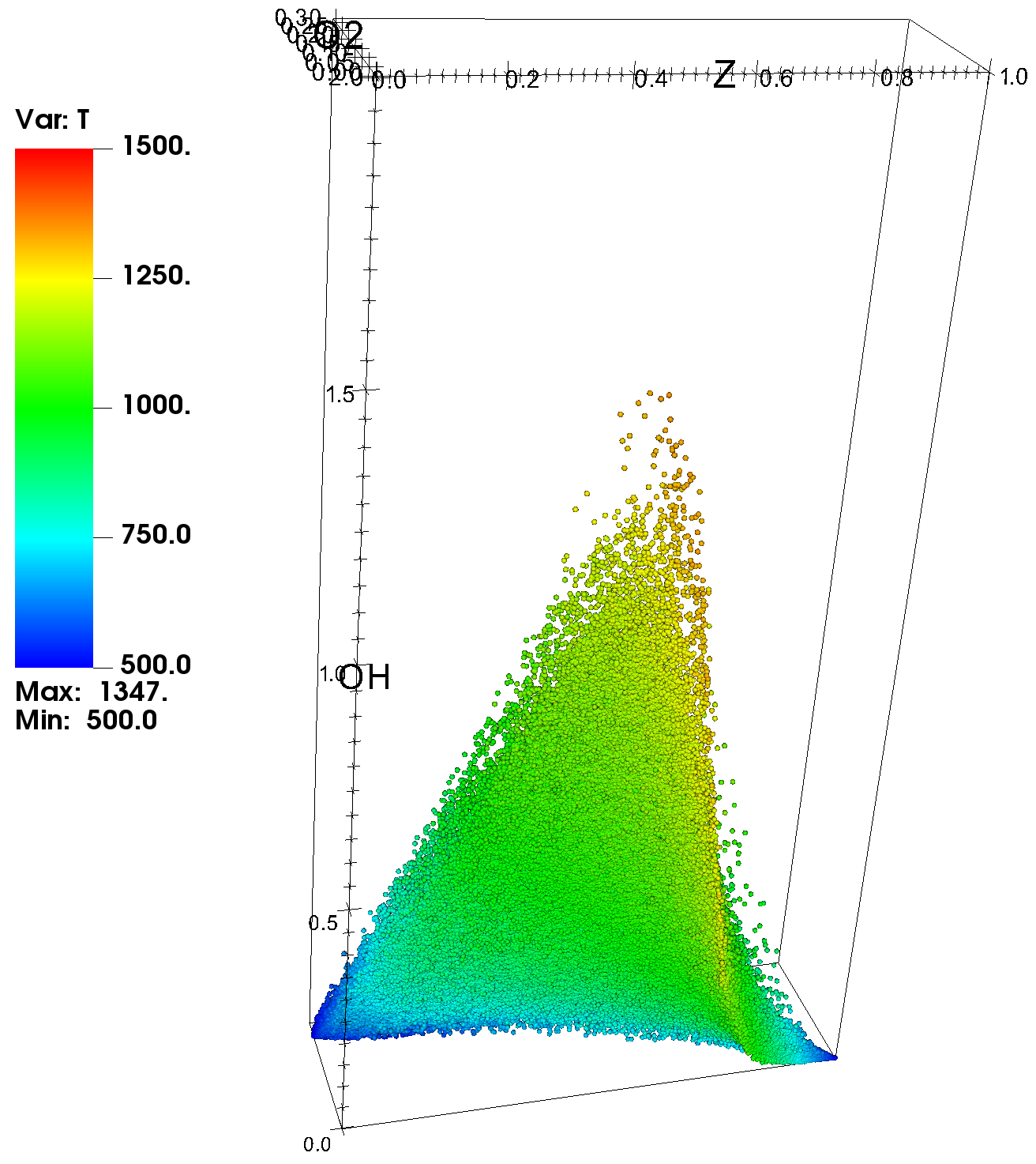
(a) $t=20tj$

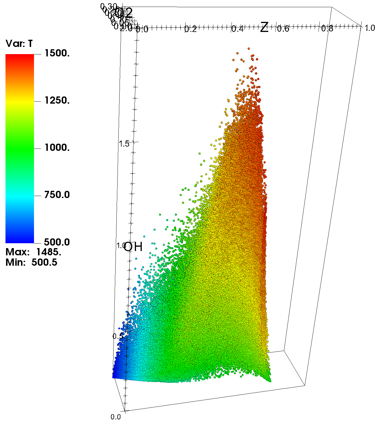
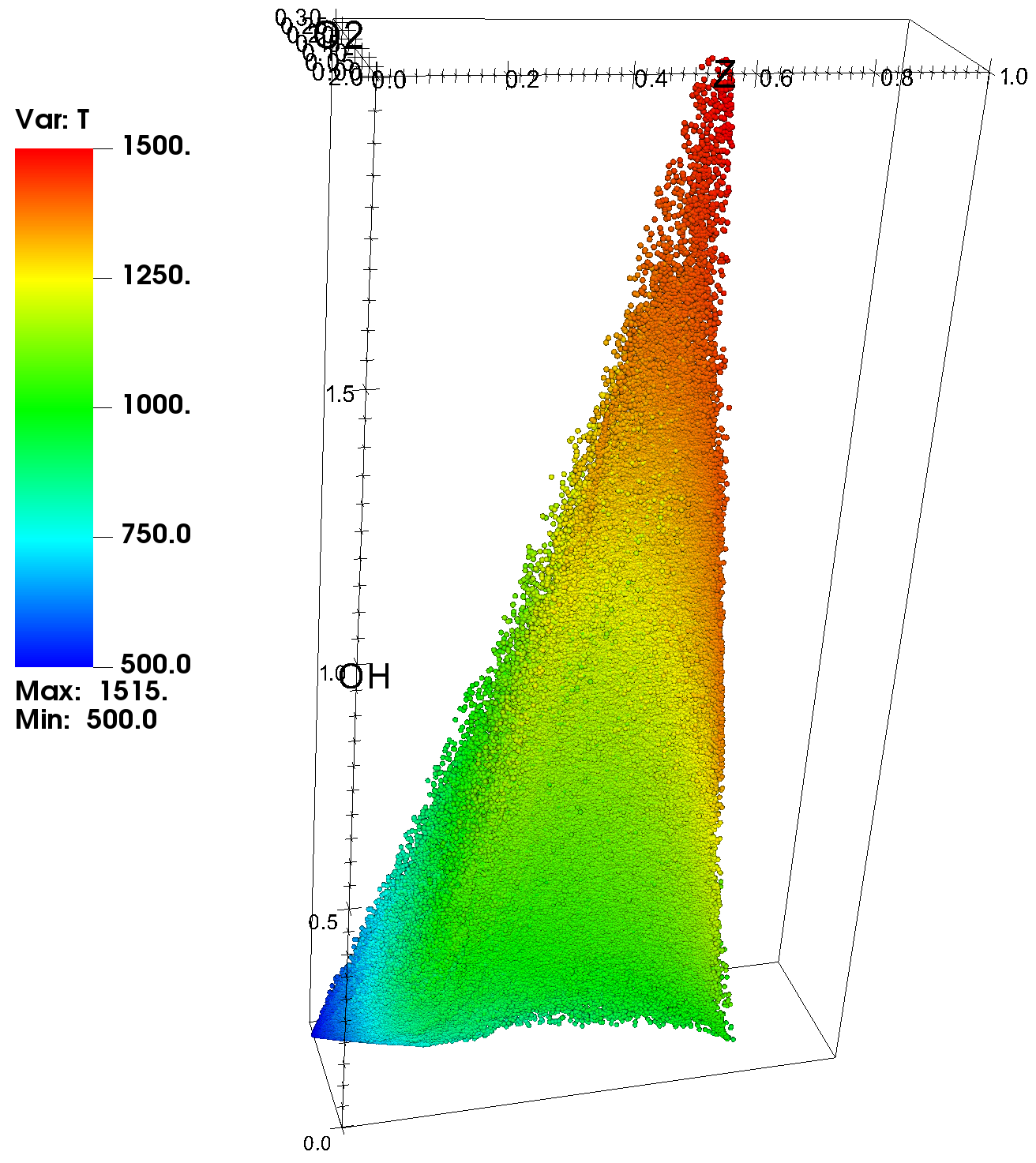
(b) $t=40tj$

Figure 14: Scatter plot of mixture fraction $Z$, oxidant mass fraction $Y_{O_{2}}$, and hydroxyl radical mass fraction $Y_{OH}\times 1000$ colored by temperature of DNS (left) and LES (right).

7 Conclusions

Modeling of turbulence-combustion interactions has been the subject of broad investigations for over seventy years now [35]. Large eddy simulation (LES) has been long recognized as a convenient means of capturing the unsteady evolution of turbulence in both non-reacting and reactive flows [28]. The major issues associated with LES for prediction of practical turbulent combustion problems are: reliable modeling of the subgrid scale (SGS) quantities, high fidelity solution of the modeled transport equations, and versatility in dealing with complex flames. The filtered density function (FDF) [29, 34, 62, 43, 68] has proven particularly effective in resolving the first issue. The present work makes a some progress in dealing with the other two. This progress is facilitated by developing a novel computational scheme by the merger of the PeleLM flow solver [19, 49, 55] and the Monte-Carlo (FDF) simulator. The resulting computational scheme facilitates reliable and high fidelity simulation of turbulent combustion systems. The novelty of the methodology, as developed, is its capability to capture the very intricate dynamics of turbulence-chemistry interactions. This is demonstrated by its implementation to conduct LES of a CO/H₂ temporally developing jet flame. The results are assessed via detailed a posteriori comparative assessments against direct numerical simulation (DNS) data for the same flame [33]. Excellent agreements are observed for the temporal evolution of all of the thermo-chemical variables, including the manifolds portraying the multi-scalar mixing. The new methodology is shown to be particularly effective in capturing non-equilibrium turbulence-chemistry interactions. This is demonstrated by capturing the flame-extinction and its re-ignition as observed in DNS. With its high fidelity and computational affordability, the new PeleLM-FDF simulator as developed here provides an excellent tool for computational simulations of complex turbulent combustion systems.

At this point it is instructive to provide some suggestions for future work in continuation of this research:

1. The hydrodynamic SGS closure adopted here is based on the zero-order model of Vreman [79]. This model has proven very effective for LES of many flows, including the one considered here. However, for more complex flows one may need to use more comprehensive SGS closures. Therefore, the extension to include the velocity-FDF [27, 71, 72, 73] is encouraged.

2. A very attractive feature of the PeleLM is its adaptive gridding and mesh refinement strategy. This feature is not utilized here because of the relative flow simplicity. Future work is needed to refine the MC strategy in conjunction with AMR. Some progress in this regard has been reported [16, 13].

3. The PeleC code [74] is the counterpart of PeleLM for high speed flows. It would be desirable to implement the FDF methodology in this code as well. In doing so, the full self-contained form of the FDF [52] should be considered.

4. Resolution assessment in LES is of crucial importance. Several such studies have been conducted for other forms of LES-FDF [22, 48, 65], and is recommended for PeleLM-FDF.

5. With its flexibility and high fidelity, it is expected that the PeleLM-FDF methodology will be implemented for LES of a wide variety of other complex turbulent combustion systems.

References

- [1] A. A. Aldama, Filtering techniques for turbulent flow simulations, in Lecture Notes in Engineering, C. A. Brebbia and S. A. Orszag, eds., vol. 49 of Lecture Notes in Engineering, Springer-Verlag, New York, NY, 1990, https://doi.org/10.1007/978-3-642-84091-3.
- [2] A. S. Almgren, J. B. Bell, P. Colella, L. H. Howell, and M. L. Welcome, A conservative adaptive projection method for the variable density incompressible Navier-Stokes equations, Journal of Computational Physics, 142 (1998), pp. 1–46, https://doi.org/10.1006/jcph.1998.5890.
- [3] N. Ansari, G. M. Goldin, M. R. H. Sheikhi, and P. Givi, Filtered density function simulator on unstructured meshes, Journal of Computational Physics, 230 (2011), pp. 7132–7150, https://doi.org/10.1016/j.jcp.2011.05.015.
- [4] N. Ansari, F. A. Jaberi, M. R. H. Sheikhi, and P. Givi, Filtered density function as a modern CFD tool, in Engineering Applications of Computational Fluid Dynamics: Volume 1, A. R. S. Maher, ed., International Energy and Environment Foundation, 2011, ch. 1, pp. 1–22.
- [5] N. Ansari, P. H. Pisciuneri, P. A. Strakey, and P. Givi, Scalar-filtered mass-density-function simulation of swirling reacting flows on unstructured grids, AIAA Journal, 50 (2012), pp. 2476–2482, https://doi.org/10.2514/1.J051671.
- [6] N. Ansari, P. A. Strakey, G. M. Goldin, and P. Givi, Filtered density function simulation of a realistic swirled combustor, Proceedings of the Combustion Institute, 35 (2015), pp. 1433–1442, https://doi.org/10.1016/j.proci.2014.05.042.
- [7] A. Aspden, M. Day, and J. Bell, Three-dimensional direct numerical simulation of turbulent lean premixed methane combustion with detailed kinetics, Combustion and Flame, 166 (2016), pp. 266–283, https://doi.org/10.1016/j.combustflame.2016.01.027.
- [8] A. J. Aspden, M. S. Day, and J. B. Bell, Towards the distributed burning regime in turbulent premixed flames, Journal of Fluid Mechanics, 871 (2019), p. 1–21, https://doi.org/10.1017/jfm.2019.316.
- [9] J. Bell, AMR for low Mach number reacting flow, in Adaptive Mesh Refinement - Theory and Applications, T. Plewa, T. Linde, and V. Gregory Weirs, eds., Springer Berlin Heidelberg, Berlin, Heidelberg, 2005, pp. 203–221, https://doi.org/10.1007/3-540-27039-6_14.
- [10] J. B. Bell, M. S. Day, A. S. Almgren, M. J. Lijewski, and C. A. Rendleman, A parallel adaptive projection method for low Mach number flows, International Journal for Numerical Methods in Fluids, 40 (2002), pp. 209–216, https://doi.org/10.1002/fld.310.
- [11] R. W. Bilger, The structure of diffusion flames, Combustion Science and Technology, 13 (1976), pp. 155–170, https://doi.org/10.1080/00102207608946733.
- [12] P. N. Brown, G. D. Byrne, and A. C. Hindmarsh, VODE: A variable-coefficient ODE solver, SIAM Journal on Scientific and Statistical Computing, 10 (1989), pp. 1038–1051, https://doi.org/10.1137/0910062.
- [13] L. P. d. Castro, A. P. Pinheiro, V. Vilela, G. M. Magalhães, R. Serfaty, and J. M. Vedovotto, Implementation of a hybrid Lagrangian filtered density function–large eddy simulation methodology in a dynamic adaptive mesh refinement environment, Physics of Fluids, 33 (2021), p. 045126, https://doi.org/10.1063/5.0045873.
- [14] S. Chibbaro, C. Marchioli, M. V. Salvetti, and A. Soldati, Particle tracking in LES flow fields: Conditional Lagrangian statistics of filtering error, Journal of Turbulence, 15 (2014), pp. 22–33, https://doi.org/10.1080/14685248.2013.873541.
- [15] P. J. Colucci, F. A. Jaberi, P. Givi, and S. B. Pope, Filtered density function for large eddy simulation of turbulent reacting flows, Physics of Fluids, 10 (1998), pp. 499–515, https://doi.org/10.1063/1.869537.
- [16] M. M. R. Damasceno, J. G. de Freitas Santos, and J. M. Vedovoto, Simulation of turbulent reactive flows using a FDF methodology – advances in particle density control for normalized variables, Computers & Fluids, 170 (2018), pp. 128–140, https://doi.org/10.1016/j.compfluid.2018.05.004.
- [17] D. Dasgupta, W. Sun, M. Day, A. J. Aspden, and T. Lieuwen, Analysis of chemical pathways and flame structure for n-dodecane/air turbulent premixed flames, Combustion and Flame, 207 (2019), pp. 36–50, https://doi.org/10.1016/j.combustflame.2019.05.026.
- [18] D. Dasgupta, W. Sun, M. Day, and T. Lieuwen, Effect of turbulence-chemistry interactions on chemical pathways for turbulent hydrogen-air premixed flames, Combustion and Flame, 176 (2017), pp. 191–201, https://doi.org/10.1016/j.combustflame.2016.09.029.
- [19] M. S. Day and J. B. Bell, Numerical simulation of laminar reacting flows with complex chemistry, Combustion Theory and Modelling, 4 (2000), pp. 535–556, https://doi.org/10.1088/1364-7830/4/4/309.
- [20] Y. P. de Almeida and S. Navarro-Martinez, Large eddy simulation of a supersonic lifted flame using the Eulerian stochastic fields method, Proceedings of the Combustion Institute, 37 (2019), https://doi.org/10.1016/j.proci.2018.08.040.
- [21] Z. Dragojlovic, F. Najmabadi, and M. Day, An embedded boundary method for viscous, conducting compressible flow, Journal of Computational Physics, 216 (2006), pp. 37–51, https://doi.org/10.1016/j.jcp.2005.11.025.
- [22] T. G. Drozda, M. R. H. Sheikhi, C. K. Madnia, and P. Givi, Developments in formulation and application of the filtered density function, Flow, Turbulence and Combustion, 78 (2007), pp. 35–67, https://doi.org/10.1007/s10494-006-9052-4.
- [23] L. Esclapez, V. Ricchiuti, J. B. Bell, and M. S. Day, A spectral deferred correction strategy for low Mach number reacting flows subject to electric fields, Combustion Theory and Modelling, 24 (2020), pp. 194–220, https://doi.org/10.1080/13647830.2019.1668060.
- [24] C. W. Gardiner, Handbook of stochastic methods for physics, chemistry and the natural sciences, Springer-Verlag, New York, NY, second ed., 1990.
- [25] E. Garnier, N. Adams, and P. Sagaut, Large eddy simulation for compressible flows, Springer Science & Business Media, 2009, https://doi.org/10.1007/978-90-481-2819-8.
- [26] M. Germano, A statistical formulation of dynamic model, Physics of Fluids, 8 (1996), pp. 565–570, https://doi.org/10.1063/1.868841.
- [27] L. Y. M. Gicquel, P. Givi, F. A. Jaberi, and S. B. Pope, Velocity filtered density function for large eddy simulation of turbulent flows, Physics of Fluids, 14 (2002), pp. 1196–1213, https://doi.org/10.1063/1.1436496.
- [28] P. Givi, Model-free simulations of turbulent reactive flows, Progress in Energy and Combustion Science, 15 (1989), pp. 1–107, https://doi.org/10.1016/0360-1285(89)90006-3.
- [29] P. Givi, Filtered density function for subgrid scale modeling of turbulent combustion, AIAA Journal, 44 (2006), pp. 16–23, https://doi.org/10.2514/1.15514.
- [30] P. Givi, W.-H. Jou, and R. Metcalfe, Flame extinction in a temporally developing mixing layer, Symposium (International) on Combustion, 21 (1986), pp. 1251–1261, https://doi.org/10.1016/S0082-0784(88)80356-4.
- [31] F. P. Hamon, M. S. Day, and M. L. Minion, Concurrent implicit spectral deferred correction scheme for low-Mach number combustion with detailed chemistry, Combustion Theory and Modelling, 23 (2019), pp. 279–309, https://doi.org/10.1080/13647830.2018.1524156.
- [32] E. Hawkes, R. Sankaran, and J. Chen, Reignition dynamics in massively parallel direct numerical simulations of CO/H2 jet flames, in 16th Australasian Fluid Mechanics Conference, School of Engineering, The University of Queensland, 2007, https://people.eng.unimelb.edu.au/imarusic/proceedings/16/Hawkes.pdf.
- [33] E. R. Hawkes, R. Sankaran, J. C. Sutherland, and J. H. Chen, Scalar mixing in direct numerical simulations of temporally evolving plane jet flames with skeletal CO/H2 kinetics, Proceedings of the Combustion Institute, 31 (2007), pp. 1633–1640, https://doi.org/10.1016/j.proci.2006.08.079.
- [34] D. C. Haworth, Progress in probability density function methods for turbulent reacting flows, Progress in Energy and Combustion Science, 36 (2010), pp. 168–259, https://doi.org/10.1016/j.pecs.2009.09.003.
- [35] W. R. Hawthorne, D. S. Weddell, and H. C. Hottel, Mixing and combustion in turbulent gas jets, Third Symposium on Combustion and Flame and Explosion Phenomena, 3 (1948), pp. 266–288, https://doi.org/10.1016/S1062-2896(49)80035-3.
- [36] A. C. Hindmarsh, P. N. Brown, K. E. Grant, S. L. Lee, R. Serban, D. E. Shumaker, and C. S. Woodward, SUNDIALS: Suite of nonlinear and differential/algebraic equation solvers, ACM Transactions on Mathematical Software, 31 (2005), p. 363–396, https://doi.org/10.1145/1089014.1089020.
- [37] M. Inkarbekov, A. Aitzhan, A. Kaltayev, and S. Sammak, A GPU-accelerated filtered density function simulator of turbulent reacting flows, International Journal of Computational Fluid Dynamics, 34 (2020), pp. 381–396, https://doi.org/10.1080/10618562.2020.1787996.
- [38] F. A. Jaberi, P. J. Colucci, S. James, P. Givi, and S. B. Pope, Filtered mass density function for large-eddy simulation of turbulent reacting flows, Journal of Fluid Mechanics, 401 (1999), pp. 85–121, https://doi.org/10.1017/S0022112099006643.
- [39] A. Y. Klimenko and M. J. Cleary, Convergence to a model in sparse-Lagrangian FDF simulations, Flow, Turbulence and Combustion, 85 (2010), pp. 567–591, https://doi.org/10.1007/s10494-010-9301-4.
- [40] P. E. Kloeden, E. Platen, and H. Schurz, Numerical solution of stochastic differential equations through computer experiments, Springer-Verlag, New York, NY, 1 ed., 1994, https://doi.org/10.1007/978-3-642-57913-4.
- [41] J. Komperda, Z. Ghiasi, D. Li, A. Peyvan, F. Jaberi, and F. Mashayek, A hybrid discontinuous spectral element method and filtered mass density function solver for turbulent reacting flows, Numerical Heat Transfer, Part B: Fundamentals, 78 (2020), pp. 1–29, https://doi.org/10.1080/10407790.2020.1746608.
- [42] J. M. Mejía, F. Chejne, A. Molina, and A. Sadiki, Scalar mixing study at high-Schmidt regime in a turbulent jet flow using large-eddy simulation/filtered density function approach, Journal of Fluids Engineering, 138 (2016), p. 021205, https://doi.org/10.1115/1.4031631.
- [43] R. S. Miller and J. W. Foster, Survey of turbulent combustion models for large eddy simulations of propulsive flowfields, AIAA Journal, 54 (2016), pp. 2930–2946, https://doi.org/10.2514/1.J054740.
- [44] J. Minier, S. Chibbaro, and S. B. Pope, Guidelines for the formulation of Lagrangian stochastic models for particle simulations of single-phase and dispersed two-phase turbulent flows, Physics of Fluids, 26 (2014), p. 113303, https://doi.org/10.1063/1.4901315.
- [45] J. Musser, A. S. Almgren, W. D. Fullmer, O. Antepara, J. B. Bell, J. Blaschke, K. Gott, A. Myers, R. Porcu, D. Rangarajan, M. Rosso, W. Zhang, and M. Syamlal, MFIX-Exa: A path toward exascale CFD-DEM simulations, The International Journal of High Performance Computing Applications, (2021), pp. 1–19, https://doi.org/10.1177/10943420211009293.
- [46] H. Natarajan, P. Popov, and G. Jacobs, A high-order semi-Lagrangian method for the consistent Monte-Carlo solution of stochastic Lagrangian drift–diffusion models coupled with Eulerian discontinuous spectral element method, Computer Methods in Applied Mechanics and Engineering, 384 (2021), p. 114001, https://doi.org/10.1016/j.cma.2021.114001.
- [47] M. B. Nik, S. L. Yilmaz, P. Givi, M. R. H. Sheikhi, and S. B. Pope, Simulation of Sandia flame D using velocity-scalar filtered density function, AIAA Journal, 48 (2010), pp. 1513–1522, https://doi.org/10.2514/1.50239.
- [48] M. B. Nik, S. L. Yilmaz, M. R. H. Sheikhi, and P. Givi, Grid resolution effects on VSFMDF/LES, Flow, Turbulence and Combustion, 85 (2010), pp. 677–688, https://doi.org/10.1007/s10494-010-9272-5.
- [49] A. Nonaka, J. B. Bell, M. S. Day, C. Gilet, A. S. Almgren, and M. L. Minion, A deferred correction coupling strategy for low Mach number flow with complex chemistry, Combustion Theory and Modelling, 16 (2012), pp. 1053–1088, https://doi.org/10.1080/13647830.2012.701019.
- [50] A. Nonaka, M. S. Day, and J. B. Bell, A conservative, thermodynamically consistent numerical approach for low Mach number combustion. Part I: Single-level integration, Combustion Theory and Modelling, 22 (2018), pp. 156–184, https://doi.org/10.1080/13647830.2017.1390610.
- [51] A. G. Nouri, P. Givi, and D. Livescu, Modeling and simulation of turbulent nuclear flames in type Ia supernovae, Progress in Aerospace Sciences, 108 (2019), pp. 156–179, https://doi.org/10.1016/j.paerosci.2019.04.004.
- [52] A. G. Nouri, M. B. Nik, P. Givi, D. Livescu, and S. B. Pope, Self-contained filtered density function, Physical Review Fluids, 2 (2017), p. 094603, https://doi.org/10.1103/PhysRevFluids.2.094603.
- [53] A. G. Nouri, S. Sammak, P. H. Pisciuneri, and P. Givi, Langevin simulation of turbulent combustion, in Combustion for Power Generation and Transportation, A. K. Agarwal, S. De, A. Pandey, and A. P. Singh, eds., Springer, 2017, ch. 3, pp. 39–53, https://doi.org/10.1007/978-981-10-3785-6_3.
- [54] E. E. O’Brien, The probability density function (PDF) approach to reacting turbulent flows, in Turbulent Reacting Flows, P. Libby and F. Williams, eds., vol. 44 of Topics in Applied Physics, Springer, Heidelberg, 1980, ch. 5, pp. 185–218, https://doi.org/10.1007/3540101926_11.
- [55] W. E. Pazner, A. Nonaka, J. B. Bell, M. S. Day, and M. L. Minion, A high-order spectral deferred correction strategy for low Mach number flow with complex chemistry, Combustion Theory and Modelling, 20 (2016), pp. 521–547, https://doi.org/10.1080/13647830.2016.1150519.
- [56] R. Pember, A. Almgren, W. Crutchfield, L. Howell, J. Bell, P. Colella, and V. Beckner, An embedded boundary method for the modeling of unsteady combustion in an industrial gas-fired furnace, in Fall meeting of the Western States Section of the Combustion Institute, Stanford, CA, 10 1995, https://www.osti.gov/biblio/195764.
- [57] R. B. Pember, L. H. Howell, J. B. Bell, P. Colella, W. Y. Crutchfield, W. A. Fiveland, and J. P. Jessee, An adaptive projection method for unsteady, low-Mach number combustion, Combustion Science and Technology, 140 (1998), pp. 123–168, https://doi.org/10.1080/00102209808915770.
- [58] N. Peters, Turbulent Combustion, Cambridge University Press, Cambridge, UK, 2000, https://doi.org/10.1017/CBO9780511612701.
- [59] P. H. Pisciuneri, S. L. Yilmaz, P. A. Strakey, and P. Givi, An irregularly portioned FDF simulator, SIAM Journal on Scientific Computing, 35 (2013), pp. C438–C452, https://doi.org/10.1137/130911512.
- [60] S. B. Pope, Computations of turbulent combustion: Progress and challenges, Proceedings of the Combustion Institute, 23 (1990), pp. 591–612, https://doi.org/10.1016/S0082-0784(06)80307-3.
- [61] S. B. Pope, Turbulent Flows, Cambridge University Press, Cambridge, U.K., 2000, https://doi.org/10.1017/CBO9780511840531.
- [62] S. B. Pope, Small scales, many species and the manifold challenges of turbulent combustion, Proceedings of the Combustion Institute, 34 (2013), pp. 1 – 31, https://doi.org/10.1016/j.proci.2012.09.009.
- [63] N. Punati, J. C. Sutherland, A. R. Kerstein, E. R. Hawkes, and J. H. Chen, An evaluation of the one-dimensional turbulence model: Comparison with direct numerical simulations of CO/H2 jets with extinction and reignition, Proceedings of the Combustion Institute, 33 (2011), pp. 1515–1522, https://doi.org/10.1016/j.proci.2010.06.127.
- [64] H. Risken, The Fokker-Planck equation, methods of solution and applications, Springer, Berlin, Heidelberg, 1996, https://doi.org/10.1007/978-3-642-61544-3.
- [65] S. Sammak, A. Aitzhan, P. Givi, and C. K. Madnia, High fidelity spectral-FDF-LES of turbulent scalar mixing, Combustion Science and Technology, 192 (2020), pp. 1219–1232, https://doi.org/10.1080/00102202.2020.1737031.
- [66] S. Sammak, M. J. Brazell, P. Givi, and D. J. Mavriplis, A hybrid DG-Monte Carlo FDF simulator, Computers & Fluids, 140 (2016), pp. 158–166, https://doi.org/10.1016/j.compfluid.2016.09.003.
- [67] S. Sammak, A. G. Nouri, M. J. Brazell, D. J. Mavriplis, and P. Givi, Discontinuous Galerkin-Monte Carlo solver for large eddy simulation of compressible turbulent flows, in 55th AIAA Aerospace Sciences Meeting, 2017, https://doi.org/10.2514/6.2017-0982.
- [68] S. Sammak, Z. Ren, and P. Givi, Modern developments in filtered density function, in Modeling and Simulation of Turbulent Mixing and Reaction: For Power, Energy and Flight, D. Livescu, A. G. Nouri, F. Battaglia, and P. Givi, eds., Springer Singapore, Singapore, 2020, pp. 181–200, https://doi.org/10.1007/978-981-15-2643-5_8.
- [69] B. A. Sen, E. R. Hawkes, and S. Menon, Large eddy simulation of extinction and reignition with artificial neural networks based chemical kinetics, Combustion and Flame, 157 (2010), pp. 566–578, https://doi.org/10.1016/j.combustflame.2009.11.006.
- [70] F. Sewerin and S. Rigopoulos, An LES-PBE-PDF approach for predicting the soot particle size distribution in turbulent flames, Combustion and Flame, 189 (2018), pp. 62–76, https://doi.org/10.1016/j.combustflame.2017.09.045.
- [71] M. R. H. Sheikhi, T. G. Drozda, P. Givi, and S. B. Pope, Velocity-scalar filtered density function for large eddy simulation of turbulent flows, Physics of Fluids, 15 (2003), pp. 2321–2337, https://doi.org/10.1063/1.1584678.
- [72] M. R. H. Sheikhi, P. Givi, and S. B. Pope, Velocity-scalar filtered mass density function for large eddy simulation of turbulent reacting flows, Physics of Fluids, 19 (2007), p. 095106, https://doi.org/10.1063/1.2768953.
- [73] M. R. H. Sheikhi, P. Givi, and S. B. Pope, Frequency-velocity-scalar filtered mass density function for large eddy simulation of turbulent flows, Physics of Fluids, 21 (2009), p. 075102, https://doi.org/10.1063/1.3153907.
- [74] H. Sitaraman, S. Yellapantula, M. T. Henry de Frahan, B. Perry, J. Rood, R. Grout, and M. Day, Adaptive mesh based combustion simulations of direct fuel injection effects in a supersonic cavity flame-holder, Combustion and Flame, 232 (2021), p. 111531, https://doi.org/10.1016/j.combustflame.2021.111531.
- [75] J. Smagorinsky, General circulation experiments with the primitive equations. I. the basic experiment, Monthly Weather Review, 91 (1963), pp. 99–164, https://doi.org/10.1175/1520-0493(1963)091<0099:GCEWTP>2.3.CO;2.
- [76] R. R. Tirunagari and S. B. Pope, LES/PDF for premixed combustion in the DNS limit, Combustion Theory and Modelling, 20 (2016), pp. 834–865, https://doi.org/10.1080/13647830.2016.1188991.
- [77] N. S. Vaghefi, M. B. Nik, P. H. Pisciuneri, and C. K. Madnia, A Priori assessment of the subgrid scale viscous/scalar dissipation closures in compressible turbulence, Journal of Turbulence, 14 (2013), pp. 43–61, https://doi.org/10.1080/14685248.2013.854901.
- [78] S. Vo, A. Kronenburg, O. T. Stein, and M. J. Cleary, MMC-LES of a syngas mixing layer using an anisotropic mixing time scale model, Combustion and Flame, 189 (2018), pp. 311–314, https://doi.org/10.1016/j.combustflame.2017.11.004.
- [79] A. W. Vreman, An eddy-viscosity subgrid-scale model for turbulent shear flow: Algebraic theory and applications, Physics of Fluids, 16 (2004), pp. 3670–3681, https://doi.org/10.1063/1.1785131.
- [80] B. Vreman, B. Geurts, and H. Kuerten, Realizability conditions for the turbulent stress tensor in large-eddy simulation, Journal of Fluid Mechanics, 278 (1994), pp. 351–362, https://doi.org/10.1017/S0022112094003745.
- [81] F. A. Williams, Turbulent combustion, in The Mathematics of Combustion, J. D. Buckmaster, ed., Frontiers in Applied Mathematics, SIAM, Philadelphia, PA, 1985, ch. 3, pp. 97–131, https://doi.org/10.1137/1.9781611971064.ch3.
- [82] S. Williams, M. Lijewski, A. Almgren, B. V. Straalen, E. Carson, N. Knight, and J. Demmel, s-step Krylov subspace methods as bottom solvers for geometric multigrid, in 2014 IEEE 28th International Parallel and Distributed Processing Symposium, 2014, pp. 1149–1158, https://doi.org/10.1109/IPDPS.2014.119.
- [83] N. T. Wimer, M. S. Day, C. Lapointe, M. A. Meehan, A. S. Makowiecki, J. F. Glusman, J. W. Daily, G. B. Rieker, and P. E. Hamlington, Numerical simulations of buoyancy-driven flows using adaptive mesh refinement: structure and dynamics of a large-scale helium plume, Theoretical and Computational Fluid Dynamics, 35 (2021), p. 61–91, https://doi.org/10.1007/s00162-020-00548-6.
- [84] S. Yang, R. Ranjan, V. Yang, W. Sun, and S. Menon, Sensitivity of predictions to chemical kinetics models in a temporally evolving turbulent non-premixed flame, Combustion and Flame, 183 (2017), pp. 224–241, https://doi.org/10.1016/j.combustflame.2017.05.016.
- [85] T. Yang, Y. Yin, H. Zhou, and Z. Ren, Review of Lagrangian stochastic models for turbulent combustion, Acta Mechanica Sinica, 37 (2021), 1349, p. 1349, https://doi.org/10.1007/s10409-021-01142-7.
- [86] Y. Yang, H. Wang, S. B. Pope, and J. H. Chen, Large-eddy simulation/probability density function modeling of a non-premixed CO/H2 temporally evolving jet flame, Proceedings of the Combustion Institute, 34 (2013), pp. 1241–1249, https://doi.org/10.1016/j.proci.2012.08.015.
- [87] S. L. Yilmaz, M. B. Nik, M. R. H. Sheikhi, P. A. Strakey, and P. Givi, An irregularly portioned Lagrangian Monte Carlo method for turbulent flow simulation, Journal of Scientific Computing, 47 (2011), pp. 109–125, https://doi.org/10.1007/s10915-010-9424-8.
- [88] L. Zhang, J. Liang, M. Sun, H. Wang, and Y. Yang, An energy-consistency-preserving large eddy simulation-scalar filtered mass density function (LES-SFMDF) method for high-speed flows, Combustion Theory and Modelling, 22 (2018), pp. 1–37, https://doi.org/10.1080/13647830.2017.1355479.
- [89] W. Zhang, A. Almgren, V. Beckner, J. Bell, J. Blaschke, C. Chan, M. Day, B. Friesen, K. Gott, D. Graves, M. Katz, A. Myers, T. Nguyen, A. Nonaka, M. Rosso, S. Williams, and M. Zingale, AMReX: A framework for block-structured adaptive mesh refinement, Journal of Open Source Software, 4 (2019), p. 1370, https://doi.org/10.21105/joss.01370.
- [90] W. Zhang, A. Almgren, M. Day, T. Nguyen, J. Shalf, and D. Unat, BoxLib with tiling: An adaptive mesh refinement software framework, SIAM Journal on Scientific Computing, 38 (2016), pp. S156–S172, https://doi.org/10.1137/15M102616X.
- [91] X. Zhao, H. Kolla, P. Zhang, B. Wu, S. Calello, and H. N. Najm, A transported probability density function method to propagate chemistry uncertainty in reacting flow CFD, in 57th AIAA Aerospace Sciences Meeting, San Diego, CA, January 7–11 2019, AIAA, pp. 1–12, https://doi.org/10.2514/6.2019-2007.
- [92] H. Zhou, S. Li, Z. Ren, and D. H. Rowinski, Investigation of mixing model performance in transported PDF calculations of turbulent lean premixed jet flames through Lagrangian statistics and sensitivity analysis, Combustion and Flame, 181 (2017), pp. 136–148, https://doi.org/10.1016/j.combustflame.2017.03.011.
- [93] H. Zhou, T. Yang, and Z. Ren, Differential diffusion modeling in LES/FDF simulations of turbulent flames, AIAA Journal, 57 (2019), pp. 3206–3212, https://doi.org/10.2514/1.J058524.