Selective Inhibition and Recruitment in Linear-Threshold Thalamocortical Networks

Abstract

Neuroscientific evidence shows that for most brain networks all pathways between cortical regions either pass through the thalamus or a transthalamic parallel route exists for any direct corticocortical connection. This paper seeks to formally study the dynamical behavior of the resulting thalamocortical brain networks with a view to characterizing the inhibitory role played by the thalamus and its benefits. We employ a linear-threshold mesoscale model for individual brain subnetworks and study both hierarchical and star-connected thalamocortical networks. Using tools from singular perturbation theory and switched systems, we show that selective inhibition and recruitment can be achieved in such networks through a combination of feedback and feedforward control. Various simulations throughout the exposition illustrate the benefits resulting from the presence of the thalamus regarding failsafe mechanisms, required control magnitude, and network performance.

I Introduction

The brain is a complex network composed of billions of individual neurons, with their interconnections forming subnetworks that perform a myriad of different functions. Communication of information between regions and its subsequent processing is one such function. Brain regions, such as the neocortex for example, have a hierarchical structure in which different cognitive levels operate on distinct timescales. Within this hierarchy, information travels from faster lower-level sensory brain regions to slower higher-level cognitive brain regions (bottom-up communication). Upon processing in the higher-level regions, information regarding decisions made by these regions is passed back down the hierarchy to perform some task (top-down communication). In this process, certain regions are selectively recruited to perform the given task, while other areas are selectively inhibited to ignore other inputs into the brain network.

Such hierarchies are not restricted to the neocortex, and neither top-down and bottom-up communications occur entirely inside the neocortex. In fact, most, if not all, direct corticocortical communications have a parallel transthalamic pathway upon which the information is transmitted and modulated [1]. Our goal here is to understand the role of transthalamic communication in enabling selective attention, with a view to characterizing its benefits. We seek to provide a dynamical explanation of this phenomena and validate the hypothesis that selective inhibition and recruitment are feasible in thalamocortical networks via feedback and feedforward mechanisms.

Literature Review: The hierarchical organization of the brain has been known for decades [2, 3] and has been extensively studied from different viewpoints [4, 5, 6, 7, 8]. The role of the communication between the thalamus and cortical regions in a thalamocortical hierarchy is a more recently studied problem. Historically, the thalamus has been viewed as a relay of sensory signals to the cortex. However, in recent literature, it has been shown to also play a further role in cognitive processes [9]. In particular, [1, 10] show that the thalamus transfers both sensory signals to the cortex using first-order relays, but that for most direct corticocortical connection, there exists a parallel transthalamic path made of higher-order thalamic relays. Further evidence is given that these paths operate using feedforward inhibitory control to communicate information from thalamic to cortical areas [11, 12, 13, 14, 15]. The works [16, 11] show that depending on the purpose (e.g., visual, auditory, somatomotor) of the hierarchical network, the thalamus connects to the hierarchy at different levels. In general, little theoretical understanding is available about the network properties of thalamocortical structures and their role in the hierarchical nature of the brain. To address this gap, here we employ linear-threshold dynamics [17, 18] as a mesoscale model for the behavior of neuronal populations and build on the hierarchical selective recruitment framework introduced in [19, 20] for corticocortical networks. The latter provides us with a baseline to compare against when analyzing the properties and performance of thalamocortical networks. We also rely on results from switched piecewise and affine systems [21, 22] and singular perturbation theory [23, 24, 25].

Statement of Contributions: We deal with thalamocortical brain networks where each brain region is governed by a linear-threshold rate dynamics. Given our focus on selective attention, the neuronal populations in each region are divided into task-relevant and task-irrelevent nodes. Inspired by the types of pathways in thalamic circuitry, we consider two interconnections topologies, multilayer hierarchical networks and star-connected networks. Our first contribution provides an analysis of selective inhibition and recruitment in hierarchical thalamocortical networks. We establish that the equilibrium maps of individual layers can be described as piecewise-affine maps. Using singular perturbation theory for non-smooth differential equations, we provide conditions for the existence of feedback-feedforward control laws that achieve selective inhibition and recruitment of the desired nodes. Our second contribution deals with star-connected thalamocortical networks, both with and without timescale separation between regions. For the latter class, we build on a generalization of stability results on slowly varying nonlinear systems to the case of exponential stability to provide conditions for the existence of a feedback-feedforward controller providing selective inhibition and recruitment. We achieve analogous results for the case of star-connected networks with timescale separation using again singular perturbation theory. Examples illustrate the beneficial role played by the thalamus in these networks with respect to metrics such as failsafe mechanisms, control magnitude, and network performance.

II Neuroscientific Background

Here we provide a summary of the neuroscientific background behind the modeling assumptions adopted in the paper. We focus on observations about brain organization, information transmission among brain regions, and the role that the thalamus is believed to play.

Task-Relevant and Task-Irrelevant Neuron Populations: in the nervous system, stimuli are represented using series of electric spikes generated by neurons that travel down nerve fibres [26]. A given stimulus is defined by a characteristic pattern of spikes traveling between neurons, which can also be represented as the firing rate of the neurons over time. In such a representation, some neurons generate spikes (have a non-zero firing rate) during the transmission of the stimuli, known as being excited, while other neurons do not (have a firing rate of zero), which is referred to as being inhibited. We refer to the subset of neuron populations that are excited during the transmission of a stimuli as the ‘task-relevant’ nodes and the remaining populations as the ‘task-irrelevant’ nodes.

Information Pathways: in the brain, there exist information pathways between different spatial regions allowing for the transmission of stimuli between processing areas. The transmission of information can be seen as the activity in one region (that is, the firing rates of the neuron populations defined by the stimuli) driving the activity in the following region by exciting the task-relevant nodes and inhibiting the task-irrelevant nodes to propagate the stimuli (and any processing of it) through the pathway. This enables the brain to generate appropriate responses to the stimuli by propagating a response through the information pathway. This response, with its own set of task relevant/irrelevant nodes, selectively recruits (excites) the task-relevant nodes, and selectively inhibits the task-irrelevant nodes. Information pathways between brain regions form both spatial and temporal hierarchies, allowing for different levels of processing occurring in different regions [27]. The temporal timescales are directly related to the complexity of processing occurring in a given region. For a low-level sensory area, where the inputs are brief and are processed quickly, the timescales are fast. Meanwhile, further up the information pathway, in regions such as the prefrontal cortex, higher-level cognitive processes use more complex inputs from earlier in the pathway by integrating them over time, resulting in slower timescales [17]. These pathways have been studied in strictly cortical networks [17, 19, 20]. However, elements of such networks also have multiple connections to the thalamus while maintaining a temporal hierarchy [1], leading to the interest here in the role of the thalamus.

(a) hierarchical thalamocortical network

(b) star-connected thalamocortical network

Figure 1: Topologies for thalamocortical networks considered in the paper. In (a), each layer is connected directly to the thalamus, as well as the layers directly above and below it. In (b), each layer is connected to the thalamus, but no direct connections exist between cortical regions. In both plots, task-relevant excitatory and inhibitory nodes are depicted in red and blue, resp., and task-irrelevant nodes are depicted in grey.

Pathways between the Thalamus and Cortical Regions: in studying thalamocortical networks, we consider two topologies of interest, cf. Fig. 1. Both share the common trait that each cortical layer is connected to the thalamus layer: however, connections between cortical layers differ in each case. These topologies are inspired by the fact that pathways in thalamic circuitry can be identified into two classes [28]. The first represents the role of the thalamus as a modulator of information being passed between cortical regions along a transthalamic route parallel to the existing corticocortical information pathways (higher-order relay) [1]. Since these cortical regions then form a temporal hierarchy, this leads to the hierarchical thalamocortical network shown in Fig. 1(a). The second class represents the thalamus as the main route for the transfer of information between two (or more) brain areas. In this case, the thalamus is relaying an input to the cortical regions (first-order relay) [1], which gives rise to the star-connected network shown in Fig. 1(b). The cortical regions to which information is being relayed can be parts of separate temporal hierarchies, however, as the regions in the network do not form a temporal hierarchy themselves, the timescales of the subnetworks are not directly related.

Role of the Thalamus: The neuroscientific literature [13] discusses a number of potential roles for the thalamus. The thalamus can significantly increase the information contained in signals both being transmitted to and between cortical regions [1]. In hierarchical networks within the cortex, transthalamic pathways allow for layers near the top of the hierarchy to directly receive the outputs from the lower levels, in addition to the more processed inputs they receive from other cortical regions [13]. Thalamic signals into the higher cortical regions can also allow for receiving further details of motor signals, such as distinguishing between self-induced stimuli (such as those generated by eye movements) and stimuli from the external environment [1]. The thalamus also has a role in controlling recurrent cortical dynamics, as the cortical networks are not able to self-sustain activity [29, 12]. Other roles include contributions to learning, memory, decision-making and inhibitory control [30, 31].

III Problem Setup

We start by providing details on the dynamic modeling of the thalamocortical network layers, then describe the effect that the interconnection topology has on the input to each layer, and finally formalize the problem under consideration.

III-A Network Modeling

We consider a thalamocortical network $\mathcal{N}$ composed of $N$ cortical layers and the thalamus. We use linear-threshold rate dynamics to model the evolution of each region in the network. These dynamics provide a mesoscale model of the evolution of the average firing rate of populations of neurons, rather than individual spike trains, by looking at the electrical currents flowing through synaptic connections, see [26]. The dynamics of cortical layer $\mathcal{N}_{i}$ composed of $n_{i}$ nodes are

$$\tau_{i}\dot{\mathbf{x}}_{i}=-\mathbf{x}_{i}+[\mathbf{W}_{i}\mathbf{x}_{i}+\mathbf{d}_{i}(t)]_{\mathbf{0}}^{\mathbf{m}_{i}}\qquad\mathbf{0}\leq\mathbf{x}_{i}(0)\leq\mathbf{m}_{i},$$ (1)

where $\mathbf{x}_{i}\in\mathbb{R}_{\geq 0}^{n_{i}}$ represents the state of the nodes within the layer, and each component of $\mathbf{x}_{i}$ represents a population of neurons with similar firing rate. The matrix $\mathbf{W}_{i}\in\mathbb{R}^{n_{i}\times n_{i}}$ is the synaptic connectivity between neuron populations within the layer and $\mathbf{d}_{i}(t)\in\mathbb{R}^{n_{i}}$ encapsulates the input into the model,

$$\mathbf{d}_{i}(t)=\mathbf{w}_{i}(t)+\mathbf{B}_{i}\mathbf{u}_{i}(t)+\mathbf{c}_{i}.$$ (2)

Here $\mathbf{w}_{i}(t)$ models the interconnections between layers, $\mathbf{u}_{i}(t)$ is the control used for the $n_{i}$ nodes in $\mathcal{N}_{i}$, and $\mathbf{c}_{i}$ includes any unmodeled background activity or external inputs. Finally $\tau_{i}\in\mathbb{R}_{\geq 0}^{n_{i}}$ is the timescale of the dynamics.

In our study, the control $\mathbf{u}_{i}$ inhibits $r_{i}\leq n_{i}$ task-irrelevant nodes (drives their state to zero), while the remaining terms in (2) recruit the remaining $n_{i}-r_{i}$ nodes and determine the desired equilibrium or trajectory. To distinguish between task-relevant and task-irrelevant nodes, we use the following partition of network variables in each layer $\mathcal{N}_{i}$,

$$\mathbf{x}_{i}=\begin{bmatrix}\mathbf{x}_{i}^{0}\\ \mathbf{x}_{i}^{1}\end{bmatrix}\qquad\mathbf{W}_{i} =\begin{bmatrix}\mathbf{W}_{i}^{00}&\mathbf{W}_{i}^{01}\\ \mathbf{W}_{i}^{10}&\mathbf{W}_{i}^{11}\end{bmatrix}$$ (3a)

$$\mathbf{B}_{i}=\begin{bmatrix}\mathbf{B}_{i}^{0}\\ \mathbf{0}\end{bmatrix}\qquad\mathbf{c}_{i} =\begin{bmatrix}\mathbf{c}_{i}^{0}\\ \mathbf{c}_{i}^{1}\end{bmatrix}\qquad\mathbf{m}_{i}=\begin{bmatrix}\mathbf{m}_{i}^{0}\\ \mathbf{m}_{i}^{1}\end{bmatrix},$$ (3b)

where $\mathbf{x}_{i}^{0}\in\mathbb{R}_{\geq 0}^{r_{i}}$ represent the task-irrelevant nodes, $\mathbf{x}_{i}^{1}\in\mathbb{R}_{\geq 0}^{n_{i}-r_{i}}$ the task-relevant nodes and $\mathbf{B}_{i}\in\mathbb{R}^{n_{i}\times p_{i}}$ is such that the task-relevant nodes are not impacted by the control term $\mathbf{u}_{i}\in\mathbb{R}^{p_{i}}$. Throughout we shall assume that $p_{i}\geq r_{i}$, and that the matrices $\mathbf{B}_{i}^{0}$ have all full rank.

The thalamus layer $\mathcal{N}_{T}$ is modeled in the same way as the cortical layers with the difference appearing in the interconnection term $\mathbf{w}_{T}(t)$. A final word about the brain mechanisms for the inhibition of regions [32]. Feedforward inhibition between two layers, $\mathcal{N}_{i}$ and $\mathcal{N}_{j}$, refers to when $\mathcal{N}_{i}$ sends an inhibitory signal to $\mathcal{N}_{j}$ to achieve its goal activity pattern for $\mathcal{N}_{j}$ regardless of the current state of $\mathcal{N}_{j}$. In contrast, feedback inhibition refers to when the inhibition applied in a layer $\mathcal{N}_{i}$ is dependent upon the current activity level of the nodes desired to be inhibited [32]. We employ a combination of feedback and feedforward inhibition.

III-B Interconnection Topology Among Network Layers

We detail here the dynamical interconnection between the network layers for each of the topologies depicted in Fig. 1.

Hierarchical Thalamocortical Networks

Consider the hierarchical thalamocortical network depicted in Fig. 1(a). The hierarchical structure is encoded by the ordered timescales of the layers: $\tau_{1}\gg\tau_{2}\gg\dots\gg\tau_{N}$, prescribing progressively faster dynamics as one moves down the hierarchy. For generality, the timescale $\tau_{T}$ of the thalamus might fit anywhere within the hierarchy. For each cortical layer $\mathcal{N}_{i}$, the interconnection term $\mathbf{w}_{i}(t)$ in (2) takes the form

$$\mathbf{w}_{i}(t) =\mathbf{W}_{i,i-1}\mathbf{x}_{i-1}(t)+\mathbf{W}_{i,i+1}\mathbf{x}_{i+1}(t)+\mathbf{W}_{i,T}\mathbf{x}_{T}(t).$$ (4)

Here, the terms $\mathbf{W}_{i,i-1},\mathbf{W}_{i,i+1}$, and $\mathbf{W}_{i,T}$ represent the weights of the synaptic connections between layers $\mathcal{N}_{i}$ and $\mathcal{N}_{i-1}$, $\mathcal{N}_{i+1}$ and $\mathcal{N}_{T}$, resp. It is important to note that since the thalamus impacts the cortical regions using feedforward inhibition, the interconnection matrix between the thalamus and the cortical layer satisfies $\mathbf{W}_{i,T}\leq 0$. Substituting (4) into the linear-threshold dynamics (1), we get the dynamics for a cortical layer $\mathcal{N}_{i}$

$$\tau_{i}\dot{\mathbf{x}}_{i} =-\mathbf{x}_{i}+[\mathbf{W}_{i,i}\mathbf{x}_{i}+\mathbf{W}_{i,i-1}\mathbf{x}_{i-1}$$ (5)

$$\quad+\mathbf{W}_{i,i+1}\mathbf{x}_{i+1}+\mathbf{W}_{i,T}\mathbf{x}_{T}+\mathbf{B}_{i}\mathbf{u}_{i}(t)+\mathbf{c}_{i}]_{\mathbf{0}}^{\mathbf{m}_{i}},$$

for $i\in\{1,\dots,N\}$. For consistency $\mathbf{W}_{1,0}=\mathbf{0}=\mathbf{W}_{N,N+1}$, and we assume that $r_{1}=0$, meaning no nodes are being inhibited in the top layer of the network.

For the thalamus layer, to reflect the different connectivity it has in the network, the interconnection term $\mathbf{w}_{T}(t)$ is

$$\mathbf{w}_{T}(t)=\sum_{i=1}^{N}\mathbf{W}_{T,i}\mathbf{x}_{i}(t).$$ (6)

Here $\mathbf{W}_{T,i}$ represents the weight of the synaptic connections between layers $\mathcal{N}_{T}$ and $\mathcal{N}_{i}$ for $i\in\{1,\dots,N\}$. Then, substituting (6) into (1), the dynamics for the thalamus layer is

$$\tau_{T}\dot{\mathbf{x}}_{T} =-\mathbf{x}_{T}+[\mathbf{W}_{T}\mathbf{x}_{T}+\sum_{i=1}^{N}\mathbf{W}_{T,i}\mathbf{x}_{i}+\mathbf{B}_{T}\mathbf{u}_{T}(t)+\mathbf{c}_{T}]_{\mathbf{0}}^{\mathbf{m}_{T}}.$$ (7)

We denote the timescale ratio between layers by $\epsilon=(\epsilon_{1},\dots,\epsilon_{N},\epsilon_{T})$, where

$$\epsilon_{i}=\frac{\tau_{i}}{\tau_{i-1}},\quad\epsilon_{T}=\frac{\tau_{T}}{\min_{\tau_{j}>\tau_{T}}\tau_{j}}.$$

For a subnetwork $\mathcal{N}_{i}$ such that the thalamus timescale fits in the hierarchy directly above it, i.e. $\tau_{T}>\tau_{i}$ but there does not exist $j$ such that $\tau_{T}>\tau_{j}>\tau_{i}$, we let the timescale ratio between $\mathcal{N}_{T}$ and $\mathcal{N}_{i}$ be given by $\bar{\epsilon}_{i}={\tau_{i}}/{\tau_{T}}$.

Star-Connected Thalamocortical Networks

Consider the star-connected thalamocortical network depicted in Fig. 1(b). In contrast to the hierarchical network, this topology does not form a hierarchical timescale, and as such there is no direct relationship satisfied by the timescales. The lack of an explicit relation encodes the thalamus’ role as a sensory relay to multiple brain regions, each part of potentially unrelated temporal hierarchies. Without loss of generality, we assume subnetwork $\mathcal{N}_{1}$ represents a subcortical structure and provides the input to the network for the thalamus to relay to the other brain regions.

As such, there are no nodes in $\mathcal{N}_{1}$ that are desired to be inhibited, meaning $r_{1}=0$. We model the subcortical input subnetwork with a linear-threshold dynamics, but without an independent control term, instead modeling input changes by allowing $\mathbf{c}_{1}$ to be time-varying. That is

$$\tau_{1}\dot{\mathbf{x}}_{1}=-\mathbf{x}_{1}+[\mathbf{W}_{1,1}\mathbf{x}_{1}+\mathbf{W}_{1,T}\mathbf{x}_{T}+\mathbf{c}_{1}(t)]_{\mathbf{0}}^{\mathbf{m}_{1}}.$$ (8)

For the cortical regions $\mathcal{N}_{i}$, $i\in\{2,\dots,N\}$, the interconnection term $\mathbf{w}_{i}(t)$ is given by $\mathbf{w}_{i}(t)=\mathbf{W}_{i,T}\mathbf{x}_{T}(t)$, and we recall that as the thalamus utilizes feedforward inhibition, $\mathbf{W}_{i,T}\leq 0$. Meanwhile, the interconnection of the thalamus with the cortical regions is defined by $\mathbf{w}_{T}(t)=\sum_{i=1}^{N}\mathbf{W}_{T,i}\mathbf{x}_{i}(t)$. Then, from the linear-threshold model (1), for $i\in\{2,\dots,N\}$ the dynamics takes the form

$$\tau_{i}\dot{\mathbf{x}}_{i} =-\mathbf{x}_{i}+[\mathbf{W}_{i,i}\mathbf{x}_{i}+\mathbf{W}_{i,T}\mathbf{x}_{T}+\mathbf{B}_{i}\mathbf{u}_{i}(t)+\mathbf{c}_{i}]_{\mathbf{0}}^{\mathbf{m}_{i}},$$ (9)

$$\tau_{T}\dot{\mathbf{x}}_{T} =-\mathbf{x}_{T}+[\mathbf{W}_{T}\mathbf{x}_{T}+\sum_{i=1}^{N}\mathbf{W}_{T,i}\mathbf{x}_{i}+\mathbf{B}_{T}\mathbf{u}_{T}(t)+\mathbf{c}_{T}]_{\mathbf{0}}^{\mathbf{m}_{T}}.$$

III-C Problem Statement

For a purely cortical hierarchical brain network, selective inhibition and recruitment can be achieved using a combination of feedback and feedforward control, dependent on the subnetwork dynamics satisfying a set of stability properties, cf. [19, 20]. However, with the presence of the thalamus and given its impact on the dynamics of the individual subnetworks, such results are inapplicable. In addition, for star-connected thalamocortical topology the results do not apply, as the assumption of a hierarchical relationship between subnetwork timescales, which plays a critical role, no longer holds. As such, in this work we study the problem of selective inhibition and recruitment for thalamocortical networks, both hierarchical and star-connected, which we formalize next.

We seek to determine the existence of control mechanisms, resulting from the combination of feedback and feedforward inhibition, such that for a thalamocortical network, with either interconnection topology as described in Section III-B, each of the individual subnetworks $\mathcal{N}_{i}$ and $\mathcal{N}_{T}$ achieves selective inhibition and recruitment. In particular, we look for a control law of the form

$$\mathbf{u}_{i}(t)=\bar{\mathbf{u}}_{i}(t)+\mathbf{K}_{i}\mathbf{x}_{i}(t),$$

for each $i\in\{2,\dots,N,\}\cup\{T\}$, that results in the state of each subnetwork converging to a desired equilibrium trajectory. Solving this problem requires determining the stability properties that the dynamics of each of the individual subnetworks must satisfy to guarantee the existence of such a control law.

In addition, we seek to evaluate how the addition of the thalamus results in improved performance relative to a purely cortical network. In particular we investigate how the addition of the thalamus impacts the control magnitude needed to achieve selective inhibition and the convergence speed of the network. Further, we study differences in the hierarchical and star-connected topologies, particularly in how the latter can act as a failsafe for the former.

IV Hierarchical Thalamocortical Networks

In this section, we consider a hierarchical multilayer thalamocortical network, cf. Fig. 1(a), where the cortical layers are governed by (5) and the thalamus layer is governed by (7).

IV-A Equilibrium Maps for Individual Layers

We note that, for a general linear-threshold dynamics (1) with $\mathbf{W}\in\mathbb{R}^{n\times n}$, its equilibrium map $h:\mathbb{R}^{n}\rightarrow\mathbb{R}_{\geq 0}^{n}$

$$h(\mathbf{c})=h_{\mathbf{W},\mathbf{m}}(\mathbf{c})=\{\mathbf{x}\in\mathbb{R}_{\geq 0}^{n}~{}|~{}\mathbf{x}=[\mathbf{W}\mathbf{x}+\mathbf{c}]_{\mathbf{0}}^{\mathbf{m}}\},$$ (10)

maps a constant input $\mathbf{c}\in\mathbb{R}^{n}$ to the set of equilibria of (1). For thalamocortical networks, the timescale of the thalamus impacts the specific form of the equilibrium maps. For simplicity, we assume the thalamus lies inside the hierarchy, i.e., there exist $a,b\in\{1,\dots,N\}$ such that $b=a+1$ and $\tau_{a}\gg\tau_{T}\gg\tau_{b}$. This choice results in a layer $\mathcal{N}_{a}$ with an equilibrium map different than any that appear in the cases when the thalamus timescale is on the boundary of the hierarchy. Our results can also be stated for the latter case with appropriate adjustments to the derived control law for selective inhibition and recruitment.

The hierarchical nature of the topology plays an important role in defining these equilibrium maps. At the theoretical limit of timescale separation between two layers, the state of a given layer becomes constant at the timescale of layers lower in the hierarchy as well as being a static function of the above layer’s states. As such, when defining the equilibrium maps for a given layer, the constant input into an equilibrium map can represent the state of layers higher in the hierarchy, given that they are relative constants at that level of the dynamics. The equilibrium maps for the layers fall into three categories: below or above the thalamus, and the thalamus itself. In all cases, the maps are defined recursively from the bottom to the top of the network. At each layer, the equilibrium map takes a constant input, representing the inputs from higher levels in the hierarchy along with any external inputs to the system, and outputs the set of equilibrium values. We next give explicit expressions for the equilibrium maps of the task-relevant component of a layer in each of the categories, which we denote $h_{i}^{1}:\mathbb{R}^{n_{i}-r_{i}}\rightarrow\mathbb{R}_{\geq 0}^{n_{i}-r_{i}}$, by combining the hierarchical model described in Section III-B with (10).

Equilibrium Maps for Layers below Thalamus

We begin by considering layers below the thalamus, i.e., with $i\geq b$. Given values of $\mathbf{x}_{T}\in\mathbb{R}^{n_{T}}$ and $\mathbf{c}_{i+1}^{1}\in\mathbb{R}^{n_{i+1}-r_{i+1}}$,

$$h_{i}^{1}(\mathbf{c}) =\{\mathbf{x}_{i}^{1}~{}|~{}\mathbf{x}_{i}^{1}=[\mathbf{W}_{i,i}^{11}\mathbf{x}_{i}^{1}+\mathbf{W}_{i,i+1}^{11}h_{i+1}^{1}(\mathbf{W}_{i+1,i}^{11}\mathbf{x}_{i}^{1}$$

$$\qquad+\mathbf{W}_{i+1,T}^{11}\mathbf{x}_{T}^{1}+\mathbf{c}_{i+1}^{1})+\mathbf{c}]_{\mathbf{0}}^{\mathbf{m}_{i}^{1}}\}.$$ (11)

We note that since $\mathbf{W}_{N,N+1}=\mathbf{0}$ by convention, this recursion is well-defined for $\mathcal{N}_{N}$, the bottom layer in the network. In particular, for layer $N$, (IV-A) reduces to (10), the standard equilibrium map for linear-threshold models.

Equilibrium Map for Thalamus

Since the thalamus is connected to all the cortical layers, the recursive definition of its equilibrium map is dependent on the equilibrium maps of all of the layers below it. Due to this, using the notation of (IV-A) for writing the recursion becomes intractable for large networks. Instead, we introduce the following simplifying notation. For a layer $\mathcal{N}_{i}$, $i\in\{1,\dots,N\}$, in the thalamocortical hierarchy, let $\mathbf{x}_{i_{e}}^{1}\in\mathbb{R}_{\geq 0}^{n_{i}-r_{i}}$ be such that

$$\mathbf{x}_{i_{e}}^{1}\in h_{i}^{1}(\mathbf{W}_{i,T}^{11}\mathbf{x}_{T}^{1}+\mathbf{W}_{i,i-1}^{11}\mathbf{x}_{i-1}^{1}+\mathbf{c}_{i}^{1}).$$

Note that, despite $\mathbf{x}_{i_{e}}$ being dependent on a set of inputs, we do not specify these. As such, when this notation is used, it is implicitly assumed that the input values are given or determined in the recursion. Depending on the point in the recursion being considered, the inputs $\mathbf{x}_{T}$ and/or $\mathbf{x}_{i-1}$ will be replaced by their equilibrium values. Now, given values $\mathbf{c}_{b}^{1},\dots,\mathbf{c}_{N}^{1}$, where $\mathbf{c}_{i}^{1}\in\mathbb{R}^{n_{i}-r_{i}}$, the thalamus equilibrium map $h_{T}^{1}:\mathbb{R}^{n_{T}-r_{T}}\rightarrow\mathbb{R}_{\geq 0}^{n_{T}-r_{T}}$ is

$$h_{T}^{1}(\mathbf{c})=\{\mathbf{x}_{T}^{1}~{}|~{}\mathbf{x}_{T}^{1}=[\mathbf{W}_{T}^{11}\mathbf{x}_{T}^{1}+\sum_{j=b}^{N}\mathbf{W}_{T,j}^{11}\mathbf{x}_{j_{e}}^{1}+\mathbf{c}]_{\mathbf{0}}^{\mathbf{m}_{T}^{1}}\}.$$ (12)

Equilibrium Maps for Layers above Thalamus

We note that, in the recursive definition for the equilibrium maps above the thalamus, the inputs to the thalamus equilibrium map (12) will include equilibrium values of layers above the thalamus in the hierarchy, in addition to the equilibrium values from lower in the hierarchy. To distinguish which maps are inputting equilibrium maps in a condensed manner, we introduce the following notation. For $i\in\{1,\dots,a\}$, we let $\mathbf{x}_{T_{e(i)}}^{1}\in\mathbb{R}^{n_{T}-r_{T}}$ denote a value inside the thalamus equilibrium set satisfying

$$\mathbf{x}_{T_{e(i)}}^{1}\in h_{T}^{1}(\sum_{j=1}^{i}\mathbf{W}_{T,j}^{11}\mathbf{x}_{j}^{1}+\sum_{j=i+1}^{a}\mathbf{W}_{T,j}^{11}\mathbf{x}_{j_{e}}^{1}+\mathbf{c}_{T}^{1}).$$

Using this notation, we define the remaining equilibrium maps. We first provide the equilibrium maps for layers $\{\mathcal{N}_{i}\}_{i=1}^{a-1}$ and finish with the map for $\mathcal{N}_{a}$. For $i\in\{1,\dots,a-1\}$, given $\mathbf{c}_{i+1}^{1}\in\mathbb{R}^{n_{i}-r_{i}}$, the equilibrium map $h_{i}^{1}:\mathbb{R}^{n_{i}-r_{i}}\rightarrow\mathbb{R}_{\geq 0}^{n_{i}-r_{i}}$ is

$$h_{i}^{1}(\mathbf{c}) =\{\mathbf{x}_{i}^{1}~{}|~{}\mathbf{x}_{i}^{1}=[\mathbf{W}_{i,i}^{1,\mathrm{all}}\mathbf{x}_{i}+\mathbf{W}_{i,i+1}h_{i+1}^{1}(\mathbf{W}_{i+1,i}^{1,\mathrm{all}}\mathbf{x}_{i}+\mathbf{c}_{i+1}^{1})$$

$$\qquad+\mathbf{W}_{i,T}^{11}\mathbf{x}_{T_{e(i)}}+\mathbf{c}]_{\mathbf{0}}^{\mathbf{m}_{i}^{1}}\}.$$ (13)

The expression for the equilibrium map of the layer $\mathcal{N}_{a}$, which is directly above the thalamus, differs from the other layers due to the fact that it depends directly on a layer below the thalamus in addition to being dependent on the thalamus. Given $\mathbf{c}_{b}^{1}\in\mathbb{R}^{n_{b}-r_{b}}$, the equilibrium map $h_{a}^{1}:\mathbb{R}^{n_{a}-r_{a}}\rightarrow\mathbb{R}_{\geq 0}^{n_{a}-r_{a}}$ is

$$h_{a}^{1}(\mathbf{c}) =\{\mathbf{x}_{a}^{1}~{}|~{}\mathbf{x}_{a}^{1}=[\mathbf{W}_{a,a}^{11}\mathbf{x}_{a}^{1}+\mathbf{W}_{a,b}^{11}h_{b}^{1}(\mathbf{W}_{b,a}^{11}\mathbf{x}_{a}^{1}$$ (14)

$$\qquad+\mathbf{W}_{b,T}^{11}\mathbf{x}_{T_{e(a)}}^{1})+\mathbf{c}_{b}^{1})+\mathbf{W}_{a,T}^{11}\mathbf{x}_{T_{e(a)}}^{1}+\mathbf{c}]_{\mathbf{0}}^{\mathbf{m}_{a}^{1}}\}.$$

We conclude this section by establishing that all the equilibrium maps in the thalamocortical network (IV-A)-(14) are piecewise-affine and use this fact to justify they are globally Lipschitz too. To begin, we note that since general linear-threshold dynamics are switched affine, their equilibrium map (10) can be written in a piecewise-affine form. In particular, this equilibrium map can be written as follows

$$h(\mathbf{c}) =\{\mathbf{F}_{\sigma}\mathbf{c}+\mathbf{f}_{\sigma}~{}|~{}\mathbf{G}_{\sigma}\mathbf{c}+\mathbf{g}_{\sigma}\geq\mathbf{0},~{}\sigma\in\{0,\ell,s\}^{n}\},$$ (15)

for some matrices and vectors of the form

$$\mathbf{F}_{\sigma} =(\mathbf{I}-\Sigma^{\ell}\mathbf{W})^{-1},\qquad\mathbf{f}_{\sigma}=(\mathbf{I}-\Sigma^{\ell}\mathbf{W})^{-1}\Sigma^{\mathbf{s}}\mathbf{m},$$

$$\mathbf{G}_{\sigma} =\begin{bmatrix}\Sigma^{\ell}+\Sigma^{s}-\mathbf{I}&\Sigma^{\ell}&-\Sigma^{\ell}&\Sigma^{s}\end{bmatrix}^{\top}\mathbf{F}_{\sigma},$$

$$\mathbf{g}_{\sigma} =\begin{bmatrix}\mathbf{f}_{\sigma}^{\top}(\Sigma^{\ell}+\Sigma^{s}-\mathbf{I})&\mathbf{f}_{\sigma}^{\top}\Sigma^{\ell}&(\mathbf{m}-\mathbf{f}_{\sigma})^{\top}\Sigma^{\ell}&(\mathbf{f}_{\sigma}-\mathbf{m})^{\top}\Sigma^{s}\end{bmatrix}^{\top},$$

where $\Sigma^{\ell}$ is a diagonal matrix with $\Sigma^{\ell}_{ii}=1$ if $\sigma_{i}=\ell$ and zero otherwise, and $\Sigma^{s}$ is defined analogously. Now, since $\mathbf{W}_{N,N+1}=\mathbf{0}$, the equilibrium map for the bottom layer in the hierarchy, $h_{N}^{1}$, has the same form as (10), and hence can be written in the form (15). The following result, which is a generalization of [20, Lemma IV.1], illustrates that in fact all the equilibrium maps in the hierarchical thalamocortical network are piecewise-affine.

Lemma IV.1.

(Piecewise-affinity of equilibrium maps in hierarchical thalamocortical linear-threshold models): Let $h_{i}:\mathbb{R}^{n}\rightarrow\mathbb{R}^{n}$, $i\in\{1,\dots,k\}$, be piecewise-affine functions,

$$h_{i}(\mathbf{c})=\mathbf{F}^{i}_{\lambda_{i}}\mathbf{c}+\mathbf{f}^{i}_{\lambda_{i}},\qquad\forall\mathbf{c}\in\Psi_{\lambda_{i}}\triangleq\{\mathbf{c}~{}|~{}\mathbf{G}_{\lambda_{i}}^{i}\mathbf{c}+\mathbf{g}_{\lambda_{i}}^{i}\geq\mathbf{0}\},$$

for $\lambda_{i}\in\Lambda_{i}$, where $\Lambda_{i}$ is a finite index set such that $\bigcup_{\lambda_{i}\in\Lambda_{i}}\Psi_{\lambda_{i}}=\mathbb{R}^{n}$. Define $\Lambda=\Lambda_{1}\times\Lambda_{2}\times\dots\times\Lambda_{k}$, $\lambda=(\lambda_{1},\dots,\lambda_{k})$ and $\Psi_{\lambda}=(\Psi_{\lambda_{1}},\dots,\Psi_{\lambda_{k}})$. Given matrices $\mathbf{W}_{1},\mathbf{W}_{2}^{i},\mathbf{W}_{3}^{i}$ and vectors $\bar{\mathbf{c}}_{i},\mathbf{c}^{\prime}$ for all $i\in\{1,\dots,k\}$ assume

$$\mathbf{x}=\left[\mathbf{W}_{1}\mathbf{x}+\sum_{i=1}^{k}\mathbf{W}_{2}^{i}h_{i}(\mathbf{W}_{3}^{i}\mathbf{x}+\bar{\mathbf{c}}_{i})+\mathbf{c}^{\prime}\right]_{\mathbf{0}}^{\mathbf{m}},$$ (16)

is known to have a unique solution $\mathbf{x}^{\prime}\in\mathbb{R}^{n^{\prime}}$ for each $\mathbf{c}^{\prime}\in\mathbb{R}^{n^{\prime}}$, and let $h^{\prime}(\mathbf{c}^{\prime})$ be this solution. Then, there exists a finite index set $\Lambda^{\prime}$ and $\{(\mathbf{F}_{\lambda}^{\prime},\mathbf{f}_{\lambda}^{\prime},\mathbf{G}_{\lambda}^{\prime},\mathbf{g}_{\lambda}^{\prime})\}_{\lambda^{\prime}\in\Lambda^{\prime}}$ such that

$$h^{\prime}(\mathbf{c}^{\prime})=\mathbf{F}_{\lambda^{\prime}}^{\prime}\mathbf{c}^{\prime}+\mathbf{f}_{\lambda^{\prime}}^{\prime},\quad\forall\mathbf{c}^{\prime}\in\Psi_{\lambda^{\prime}}^{\prime}\triangleq\{\mathbf{c}^{\prime}~{}|~{}\mathbf{G}_{\lambda^{\prime}}^{\prime}\mathbf{c}^{\prime}+\mathbf{g}_{\lambda^{\prime}}^{\prime}\geq\mathbf{0}\}$$

for $\lambda^{\prime}\in\Lambda^{\prime}$ and $\bigcup_{\lambda^{\prime}\in\Lambda^{\prime}}\Psi_{\lambda^{\prime}}=\mathbb{R}^{n^{\prime}}$.

The equilibrium maps for the hierarchical thalamocortical network satisfy Lemma IV.1 with $r=1$, $r=N-b$ and $r=2$ for the layers below the thalamus, the thalamus, and the layers above the thalamus, resp., and therefore the maps are piecewise-affine. Finally, the fact that these maps are globally Lipschitz follows from [20, Lemma IV.2]. This property is necessary to be able to apply later the generalization of Tikhonov’s singular perturbation stability theorem to non-smooth ODEs given in [25, Proposition 1] to take advantage of the timescale separation between the layers.

IV-B Stability Assumptions and Conditions

In the hierarchical thalamocortical model described in Section III, only the task-irrelevant components of the dynamics are directly controlled over, cf. (3b). This means that assumptions on the stability of the task-relevant components of the dynamics are needed to guarantee their stability and recruitment to an equilibrium trajectory. In particular, we are interested in the reduced-order task-relevant dynamics, that is, the system dynamics in which the inputs from layers lower in the hierarchy have been replaced by their equilibrium values. Here, we provide details on these assumptions and identify sufficient conditions for them to hold. We split our discussion on the assumptions based upon the location of a layer in the hierarchy as different locations maintain both different roles and equilibrium maps.

Top Layer of the Hierarchy

The top layer $\mathcal{N}_{1}$ in the hierarchy does not have any nodes that are to be inhibited. In addition, its role is in driving the selective recruitment in the lower levels, rather than being recruited itself. As such, we only require that the trajectories of its dynamics are bounded. Formally, for all sets of constants $\mathbf{c}_{1}\in\mathbb{R}^{n_{1}}$, $\mathbf{c}_{i}^{1}\in\mathbb{R}^{n_{i}-r_{i}}$, $i\in\{2,\dots,N\}$, and $\mathbf{c}_{T}\in\mathbb{R}^{n_{T}-r_{T}}$, we assume

$$\tau_{1}\dot{\bar{\mathbf{x}}}_{1} =-\mathbf{x}_{1}+[\mathbf{W}_{1,1}\bar{\mathbf{x}}_{1}+\mathbf{W}_{1,2}^{11}h_{2}^{1}(\mathbf{W}_{2,1}\bar{\mathbf{x}}_{1}+\mathbf{c}_{2}^{1})$$

$$\qquad+\mathbf{W}_{1,T}^{11}\mathbf{x}_{T_{e(1)}}+\mathbf{c}_{1}]_{\mathbf{0}}^{\mathbf{m}_{1}},$$ (17)

has bounded solutions. We note that our earlier assumption that the thalamus is in the middle of the hierarchy makes the top layer a cortical one. If, instead, the thalamus was the top layer, one would instead assume here that its dynamics has bounded solutions, replacing (17) accordingly.

Lower Layers in the Hierarchy

In each of the layers below the top one, we seek to accomplish selective inhibition and recruitment by having the dynamics converge to a parameter-dependent equilibrium trajectory. For the task-irrelevant components, we aim to use a control law to stabilize them to zero. If successful, what remains is the task-relevant dynamics, which we then need to be globally exponentially stable to a parameter-dependent equilibrium trajectory. In such a case, an additional challenge is then to identify conditions on the interconnected network layers that ensure the coupled system displays the desired behavior. Due to the different reduced-order dynamics throughout the network, we provide the details for this assumption in four categories: layers above the thalamus, layer directly above the thalamus, thalamus, and layers below the thalamus.

Layers above the Thalamus

For each layer $\mathcal{N}_{i}$, with $i\in\{1,\dots,a-1\}$, above the thalamus, the dynamics are directly dependent on two layers below it, and hence the reduced-order dynamics are dependent on two equilibrium maps. For achieving selective inhibition and recruitment, we assume that, for all sets of constants $\mathbf{c}_{i+1}^{1}\in\mathbb{R}^{n_{i+1}-r_{i+1}}$, $\mathbf{c}_{i}^{1}\in\mathbb{R}^{n_{i}-r_{i}}$, and $\mathbf{c}_{j}^{1}\in\mathbb{R}^{n_{j}-r_{j}}$, $j\in\{i+2,\dots,N\}\cup\{T\}$, the reduced-order dynamics

$$\tau_{i}\dot{\mathbf{x}}_{i}^{1} =-\mathbf{x}_{i}^{1}+[\mathbf{W}_{i,i}^{11}\mathbf{x}_{i}^{1}+\mathbf{W}_{i,i+1}^{11}h_{i+1}^{1}(\mathbf{W}_{i+1,i}^{11}\mathbf{x}_{i}^{1}$$

$$\quad+\mathbf{c}_{i+1}^{1})+\mathbf{W}_{i,T}^{11}\mathbf{x}_{T_{e(i)}}+\mathbf{c}_{i}^{1}]_{\mathbf{0}}^{\mathbf{m}_{i}^{1}},$$ (18)

are GES to an equilibrium trajectory defined by the chosen constants.

Layer Directly above the Thalamus

For the layer $\mathcal{N}_{a}$ directly above the thalamus, while still dependent on two layers below it in the hierarchy, one of these layers is below the thalamus. In the reduced-order model, this changes the equilibrium maps. Thus, for all constants $\mathbf{c}_{a}^{1}\in\mathbb{R}^{n_{a}-r_{a}}$, $\mathbf{c}_{b}^{1}\in\mathbb{R}^{n_{b}-r_{b}}$, and $\mathbf{c}_{i}^{1}\in\mathbb{R}^{n_{i}-r_{i}}$, $i\in\{b+1,\dots,N\}\cup\{T\}$, we assume its reduced-order dynamics

$$\tau_{a}\dot{\mathbf{x}}_{a}^{1} =-\mathbf{x}_{a}^{1}+[\mathbf{W}_{a,a}^{11}\mathbf{x}_{a}^{1}+\mathbf{W}_{a,b}^{11}h_{b}^{1}(\mathbf{W}_{b,a}^{11}\mathbf{x}_{a}^{1}$$

$$\quad+\mathbf{W}_{b,T}\mathbf{x}_{T_{e(a)}}+\mathbf{c}_{b}^{1})+\mathbf{W}_{a,T}^{11}\mathbf{x}_{T_{e(a)}}+\mathbf{c}_{a}^{1}]_{\mathbf{0}}^{\mathbf{m}_{a}^{1}},$$ (19)

are GES to an equilibrium trajectory determined by the chosen constants.

Thalamus Layer

Since the thalamus layer depends on all the other layers in the network, its reduced-order dynamics are dependent on the $N-b$ equilibrium maps of all the layers (from $\mathcal{N}_{b}$ to $\mathcal{N}_{N}$) below the thalamus. For all constants $\mathbf{c}_{b}^{1}\in\mathbb{R}^{n_{b}-r_{b}},\dots,\mathbf{c}_{N}^{1}\in\mathbb{R}^{n_{N}-r_{N}}$ and $\mathbf{c}_{T}^{1}\in\mathbb{R}^{n_{T}-r_{T}}$, we assume the reduced-order dynamics

$$\tau_{T}\dot{\mathbf{x}}_{T}^{1} =-\mathbf{x}_{T}^{1}+\big{[}\mathbf{W}_{T}^{11}\mathbf{x}_{T}^{1}+\sum_{j=1}^{a}\mathbf{W}_{T,j}^{1,\mathrm{all}}\mathbf{x}_{j}^{1}$$

$$\quad+\sum_{j=b}^{N}\mathbf{W}_{T,j}^{11}\mathbf{x}_{j_{e}}^{1}+\mathbf{c}_{T}^{1}\big{]}_{\mathbf{0}}^{\mathbf{m}_{T}^{1}},$$ (20)

are GES to an equilibrium trajectory defined by the constants $\mathbf{c}_{b}^{1},\dots,\mathbf{c}_{N}^{1}$ and $\mathbf{c}_{T}^{1}$.

Layers below the Thalamus

Finally, the layers below the thalamus are directly dependent on only one layer below them in the hierarchy. For all constants $\mathbf{c}_{i+1}^{1}\in\mathbb{R}^{n_{i+1}-r_{i+1}}$ and $\mathbf{c}_{i}^{1}\in\mathbb{R}^{n_{i}-r_{i}}$, we assume its reduced-order dynamics

$$\tau_{i}\dot{\mathbf{x}}_{i}^{1} =-\mathbf{x}_{i}^{1}+[\mathbf{W}_{i,i}^{11}\mathbf{x}_{i}^{1}+\mathbf{W}_{i,i+1}^{11}h_{i+1}^{1}(\mathbf{W}_{i+1,i}^{1,\mathrm{all}}\mathbf{x}_{i}$$

$$\quad+\mathbf{W}_{i+1,T}^{1,\mathrm{all}}\mathbf{x}_{T}+\mathbf{c}_{i+1}^{1})+\mathbf{W}_{i,T}^{1,\mathrm{all}}\mathbf{x}_{T}+\mathbf{c}_{i}^{1}]_{\mathbf{0}}^{\mathbf{m}_{i}^{1}},$$ (21)

and we assume they are GES to an equilibrium trajectory dependent upon the constants $\mathbf{c}_{i+1}^{1}$ and $\mathbf{c}_{i}^{1}$.

We next turn our attention to identifying conditions under which the above assumptions on the individual subnetworks hold, specifically, ensuring that the reduced-order dynamics for layers $\mathcal{N}_{2},\dots,\mathcal{N}_{N},\mathcal{N}_{T}$ are GES. The following result makes use of the fact that the equilibrium maps are piecewise-affine, cf. Lemma IV.1.

Lemma IV.2.

(Sufficient condition for existence and uniqueness of equilibria and GES in multilayer linear-threshold networks with parallel connections): Let $h_{i}:\mathbb{R}^{n}\rightarrow\mathbb{R}^{n}$, $i\in\{1,\dots,K\}$, be piecewise-affine functions,

$$h_{i}(\mathbf{c})=\mathbf{F}^{i}_{\lambda_{i}}\mathbf{c}+\mathbf{f}^{i}_{\lambda_{i}},\qquad\forall\mathbf{c}\in\Psi_{\lambda_{i}}\triangleq\{\mathbf{c}~{}|~{}\mathbf{G}_{\lambda_{i}}^{i}\mathbf{c}+\mathbf{g}_{\lambda_{i}}^{i}\}$$

for all $\lambda_{i}\in\Lambda_{i}$ where $\Lambda_{i}$ is a finite index set such that $\bigcup_{\lambda_{i}\in\Lambda_{i}}\Psi_{\lambda_{i}}=\mathbb{R}^{n}$. Define $\bar{\mathbf{F}}_{i}\triangleq\max_{\lambda_{i}\in\Lambda_{i}}|\mathbf{F}^{i}_{\lambda_{i}}|$ as the matrix made of the entry-wise maximum of the elements in $\{|\mathbf{F}_{\lambda_{i}}^{i}|\}_{\lambda_{i}\in\Lambda_{i}}$. For $i\in\{1,\dots,K\}$ let the matrices $\mathbf{W}_{1}^{i},\mathbf{W}_{2}^{i},$ be arbitrary and also consider arbitrary matrix $\mathbf{W}$. Then, if

$$\rho\left(|\mathbf{W}|+\sum_{i=1}^{K}|\mathbf{W}_{1}^{i}|\bar{\mathbf{F}}_{i}|\mathbf{W}_{2}^{i}|\right)<1,$$

the dynamics

$$\tau\dot{\mathbf{x}} =-\mathbf{x}+\left[\mathbf{W}\mathbf{x}+\sum_{i=1}^{K}\mathbf{W}_{1}^{i}h_{i}(\mathbf{W}_{2}^{i}\mathbf{x}+\bar{\mathbf{c}}_{i})+\mathbf{c}\right]_{\mathbf{0}}^{\mathbf{m}}$$

is GES to a unique for all constants $\bar{\mathbf{c}}_{i},\mathbf{c}$.

Lemma IV.2 generalizes [20, Theorem IV.4] to thalamocortical networks and its proof follows a similar line of arguments. The application of this result to our setting results in, if $\rho(|\mathbf{W}_{i,i}^{11}|+|\mathbf{W}_{i,i+1}^{11}|\bar{\mathbf{F}}_{i+1}|\mathbf{W}_{i+1,i}^{11}|+|\mathbf{W}_{i,T}^{11}|\bar{\mathbf{F}}_{T}|\mathbf{W}_{T,i}^{11}|)<1$ for $i\in\{2,\dots,a-1\}$, $\rho(|\mathbf{W}_{i,i}^{11}|+|\mathbf{W}_{i,i+1}^{11}|\bar{\mathbf{F}}_{i+1}|\mathbf{W}_{i+1,i}^{11}|)<1$, for $i\in\{b,\dots,N\}$ and $\rho(|\mathbf{W}_{T}^{11}|+\sum_{i=b}^{N}|\mathbf{W}_{T,i}^{11}|\bar{\mathbf{F}}_{i}|\mathbf{W}_{i,T}^{11}|)<1$, then the dynamics (18)-(21) are GES to an equilibria.

Remark IV.3.

(Comparison with conditions for a strictly cortical hierarchical network): Sufficient conditions for GES of the reduced-order dynamics of a strictly cortical network can be obtained from the above by allowing $\mathbf{W}_{i,T}^{11}=0$ for all $i$, and then these conditions reduce to those found in [20], as expected. These sufficient conditions to guarantee GES, for layers above the thalamus, are harder to satisfy in the thalamocortical network than in a cortical one. However, as the conditions are only sufficient, this does not mean that it is in fact more difficult to achieve GES of the reduced-order dynamics in the thalamocortical case, as the proof above does not explicitly invoke the inhibitory nature of the thalamus. $\bullet$

IV-C Selective Inhibition and Recruitment

We are ready to illustrate how selective inhibition and recruitment can be achieved in the hierarchical thalamocortical network model. Here, we first formalize the concept mathematically and then provide a feedforward-feedback control that achieves it. Recall that selective inhibition corresponds to the task-irrelevant components of the network converging to zero, and recruitment corresponds to having the task-relevant components converge to an equilibrium trajectory. The timescale ratio between layers, $\epsilon$, must approach zero to encode the separation of timescales observed in the brain. As such, we require convergence of the task-relevant components of the network to an equilibrium as this ratio approaches zero. Formally, selective inhibition and recruitment is achieved if the following equations are satisfied for any $0<t_{1}<t_{2}<\infty$: first, for all layers $\mathcal{N}_{i}$, $i\in\{2,\dots,N\}\cup\{T\}$, it holds that

[inhibition]: $$\quad\lim_{\epsilon\to 0}\sup_{t\in[t_{1},t_{2}]}\left\|\mathbf{x}_{i}^{0}(t)\right\|=0;$$ (22a)

second, for the top layer $$\mathcal{N}_{1}$$ in the hierarchy,

[driving layer]: $$\quad\lim_{\epsilon\to 0}\sup_{t\in[t_{1},t_{2}]}\left\|\mathbf{x}_{1}^{1}(t)-\bar{\mathbf{x}}_{1}^{1}(t)\right\|=0;$$ (22b)

for all layers $$\{\mathcal{N}_{i}\}_{i=2}^{a}$$ above the thalamus,

[recruitment]: $$\quad\lim_{\epsilon\to 0}\sup_{t\in[t_{1},t_{2}]}\|\mathbf{x}_{i}^{1}(t)$$

$$\quad\quad-h_{i}^{1}(\mathbf{W}_{i,i-1}^{11}\mathbf{x}_{i-1}^{1}(t)+\mathbf{c}_{i}^{1})\|=0;$$ (22c)

for the thalamus layer,

[recruitment]: $$\quad\lim_{\epsilon\to 0}\sup_{t\in[t_{1},t_{2}]}\left\|\mathbf{x}_{T}^{1}(t)-x_{T_{e(a)}}\right\|=0;$$ (22d)

and finally, for the layers $$\{\mathcal{N}_{i}\}_{i=b}^{N}$$ below the thalamus,

[recruitment]: $$\quad\lim_{\epsilon\to 0}\sup_{t\in[t_{1},t_{2}]}\|\mathbf{x}_{i}^{1}(t)-h_{i}^{1}(\mathbf{W}_{i,i-1}^{1,\mathrm{all}}\mathbf{x}_{i-1}(t)$$

$$\quad\qquad+\mathbf{W}_{i,T}^{1,\mathrm{all}}\mathbf{x}_{T}(t)+\mathbf{c}_{i}^{1})\|=0.$$ (22e)

Intuitively, we note from (22) that achieving selective inhibition and recruitment means that one can make the error between the network trajectories and the equilibrium trajectories arbitrarily small if the timescale ratio is small enough. The following result shows that selective inhibition and recruitment can be achieved in the hierarchical thalamocortical network by means of a combination of feedforward and feedback control.

Theorem IV.4.

(Selective inhibition and recruitment in hierarchical thalamocortical networks with Feedforward-Feedback Control): Consider an $N$-layer thalamocortical network as shown in Fig. 1(a), with layer dynamics given by (5) and (7). Without loss of generality, let $\tau_{1}\gg\tau_{2}\gg\dots\gg\tau_{T}\gg\dots\gg\tau_{N}$ and $a,b\in\{1,\dots,N\}$ such that $\tau_{a}\gg\tau_{T}\gg\tau_{b}$, with $b=a+1$. Assume the stability conditions (17)-(21) for the reduced-order subnetworks are satisfied. Then, for $i\in\{1,\dots,N\}\cup\{T\}$ and constants $\mathbf{c}_{i}\in\mathbb{R}^{n_{i}}$ and $\mathbf{c}_{T}\in\mathbb{R}^{n_{T}}$, there exist control laws $\mathbf{u}_{i}(t)=\mathbf{K}_{i}\mathbf{x}_{i}(t)+\bar{\mathbf{u}}_{i}(t)$, with $\mathbf{K}_{i}\in\mathbb{R}^{p_{i}\times n_{i}}$ and $\bar{\mathbf{u}}_{i}:\mathbb{R}_{\geq 0}\rightarrow\mathbb{R}_{\geq 0}^{p_{i}}$, such that the closed-loop system achieves selective inhibition and recruitment (22).

Proof.

We prove the result by constructing a control and iteratively applying the generalization of Tikhonov’s theorem from [25]. Throughout the proof, we make use of the following notation. For $i\leq a$, let $\mathbf{x}_{1:i}=\begin{bmatrix}\mathbf{x}_{1}^{\top}&\dots&\mathbf{x}_{i}^{\top}\end{bmatrix}^{\top}$ and, for $i\geq b$, let $\mathbf{x}_{1:T:i}=\begin{bmatrix}\mathbf{x}_{1}^{\top}\dots\mathbf{x}_{a}^{\top}&\mathbf{x}_{T}^{\top}&\mathbf{x}_{b}^{\top}&\dots&\mathbf{x}_{i}^{\top}\end{bmatrix}^{\top}$. We first define the control for layer $\mathcal{N}_{N}$. Let $\mathbf{K}_{N}$ and $\bar{\mathbf{u}}_{N}(t)$ be such that

$$\mathbf{B}_{N}^{0}\mathbf{K}_{N} \leq-\mathbf{W}_{N,N}^{0,\mathrm{all}},$$ (23a)

$$\mathbf{B}_{N}^{0}\bar{\mathbf{u}}_{N}(t) \leq-\mathbf{W}_{N,N-1}^{0,\mathrm{all}}\mathbf{x}_{N-1}(t)-\mathbf{W}_{N,T}^{0,\mathrm{all}}\mathbf{x}_{T}(t)-\mathbf{c}_{N}^{0}.$$ (23b)

The inequalities (23) can be satisfied due to our assumption that the matrices $\mathbf{B}_{i}^{0}$ have full rank and $p_{i}\geq r_{i}$ for all $i\in\{1,\dots,N\}\cup\{T\}$. Substituting (23) into the dynamics,

$$\tau_{1}\dot{\mathbf{x}}_{1} =-\mathbf{x}_{1}+[\mathbf{W}_{1,1}\mathbf{x}_{1}+\mathbf{W}_{1,2}\mathbf{x}_{2}+\mathbf{W}_{1,T}\mathbf{x}_{T}+\mathbf{c}_{1}]_{\mathbf{0}}^{\mathbf{m}_{1}},$$

$$\vdots$$

$$\tau_{T}\dot{\mathbf{x}}_{T} =-\mathbf{x}_{T}+\bigg{[}\mathbf{W}_{T}\mathbf{x}_{T}+\sum_{j=1}^{N}\mathbf{W}_{T,j}\mathbf{x}_{j}+\mathbf{B}_{T}\mathbf{u}_{T}+\mathbf{c}_{T}\bigg{]}_{\mathbf{0}}^{\mathbf{m}_{T}},$$

$$\vdots$$

$$\epsilon_{N}\tau_{N-1}\dot{\mathbf{x}}_{N}^{0} =-\mathbf{x}_{N}^{0},$$

$$\epsilon_{N}\tau_{N-1}\dot{\mathbf{x}}_{N}^{1} =-\mathbf{x}_{N}^{1}+[\mathbf{W}_{N,N}^{1,\mathrm{all}}\mathbf{x}_{N}+\mathbf{W}_{N,N-1}^{1,\mathrm{all}}\mathbf{x}_{N-1}$$

$$\qquad+\mathbf{W}_{N,T}^{1,\mathrm{all}}\mathbf{x}_{T}+\mathbf{c}_{N}^{1}]_{\mathbf{0}}^{\mathbf{m}_{1}^{1}}.$$

Taking $\epsilon_{N}\to 0$ then provides a separation of timescales between $\mathbf{x}_{N}$ and $\mathbf{x}_{1:T:N-1}$. Note that, by assumption, the reduced-order dynamics (21) is GES. Using then the fact that the cascaded interconnection of a GES system with an exponentially vanishing system is also GES, cf. [19, Lemma A.1], we deduce that, for any constants $\mathbf{x}_{N-1}$ and $\mathbf{x}_{T}$, $\mathbf{x}_{N}$ is GES to $(\mathbf{0}_{r_{N}},h_{N}^{1}(\mathbf{W}_{N,N-1}^{1,\mathrm{all}}\mathbf{x}_{N-1}+\mathbf{W}_{N,T}^{1,\mathrm{all}}\mathbf{x}_{T}+\mathbf{c}_{N}^{1}))$. Recalling that, by Lemma IV.1 and [20, Lemma IV.2], the equilibrium maps $h_{i}^{1}$ are globally Lipschitz for all $i\in\{1,\dots,N\}\cup\{T\}$, and noting that the entire network is Lipschitz due to the Lipschitzness of the linear-threshold function $[\cdot]_{\mathbf{0}}^{\mathbf{m}}$, we can apply [25, Proposition 1], giving for $0<t_{1}<t_{2}<\infty$,

$$\lim_{\epsilon_{1}\to 0}\sup_{[t_{1},t_{2}]}\left\|\mathbf{x}_{N}^{0}(t)\right\|=0,$$

$$\lim_{\epsilon_{1}\to 0}\sup_{[t_{1},t_{2}]}\big{\|}\mathbf{x}_{N}^{1}(t)-h_{N}^{1}(\mathbf{W}_{N,N-1}^{1,\mathrm{all}}\mathbf{x}_{N-1}(t)$$

$$\qquad+\mathbf{W}_{N,T}^{1,\mathrm{all}}\mathbf{x}_{T}(t)+\mathbf{c}_{N}^{1})\big{\|}=0,$$

$$\lim_{\epsilon_{1}\to 0}\sup_{[t_{1},t_{2}]}\left\|\mathbf{x}_{1:T:N-1}-\mathbf{x}_{1:T:N-1}^{(1)}\right\|=0,$$ (24)

where $\mathbf{x}_{1:T:N-1}^{(1)}$ represents the first-step reduced-order model coming from replacing $\mathbf{x}_{N}$ by its equilibrium value $(\mathbf{0}_{r_{N}},h_{N}^{1}(\mathbf{W}_{N,N-1}^{1,\mathrm{all}}\mathbf{x}_{N-1}+\mathbf{W}_{N,T}^{1,\mathrm{all}}\mathbf{x}_{T}+\mathbf{c}_{N}^{1}))$. We continue the proof by iterating the above process for each network layer, utilizing constructed control laws and applying [25, Proposition 1] to the corresponding reduced-order models built from substitution of the equilibrium values.

We now construct control laws for layers $\mathcal{N}_{i}$ with $i\in\{b,\dots,N-1\}$. We choose $\mathbf{K}_{i}$ and $\bar{\mathbf{u}}_{i}(t)$ such that

$$\mathbf{B}_{i}^{0}\mathbf{K}_{i} \leq-|\mathbf{W}_{i,i}^{0,\mathrm{all}}|-|\mathbf{W}_{i,i+1}^{01}|\bar{\mathbf{F}}_{i+1}|\mathbf{W}_{i+1,i}^{1,\mathrm{all}}|,$$ (25a)

$$\mathbf{B}_{i}^{0}\bar{\mathbf{u}}_{i}(t) \leq-\mathbf{W}_{i,i-1}^{0,\mathrm{all}}\mathbf{x}_{i-1}(t)-\mathbf{W}_{i,T}^{0,\mathrm{all}}\mathbf{x}_{T}(t)-\mathbf{c}_{i}^{0}$$ (25b)

$$\qquad-|\mathbf{W}_{i,i+1}^{01}|\bar{\mathbf{F}}_{i+1}|\mathbf{W}_{i+1,T}^{1,\mathrm{all}}\mathbf{x}_{T}(t)+\mathbf{c}_{i+1}^{1}|,$$ (25c)

in which $\bar{\mathbf{F}}_{i}\in\mathbb{R}^{(n_{i}-r_{i})\times(n_{i}-r_{i})}$ is the entry-wise maximal gain of the equilibrium map $h_{i}^{1}(\cdot)$ as defined in Lemma IV.2. We use the control law (25) to construct the reduced-order model, consider the timescale separation by letting $\epsilon_{i}\to 0$ for $i\in\{b,\dots,N-1\}$, and finally apply [25, Proposition 1] to obtain

$$\lim_{\epsilon\to 0}\sup_{t\in[t_{1},t_{2}]}\left\|\mathbf{x}_{i}^{(N-i)^{0}}(t)\right\|=0,$$

$$\lim_{\epsilon\to 0}\sup_{t\in[t_{1},t_{2}]}\|\mathbf{x}_{i}^{(N-i)^{1}}(t)-h_{i}^{1}(\mathbf{W}_{i,i-1}^{1,\mathrm{all}}\mathbf{x}_{i-1}^{(N-i)}(t)$$

$$\qquad+\mathbf{W}_{i,T}^{1,\mathrm{all}}\mathbf{x}_{T}^{(N-i)}(t)+\mathbf{c}_{i}^{1})\|=0,$$

$$\lim_{\epsilon\to 0}\sup_{t\in[t_{1},t_{2}]}\left\|\mathbf{x}_{1:T:i-1}^{(N-i)}(t)-\mathbf{x}_{1:T:i-1}^{(N-i+1)}(t)\right\|=0,$$

for all $i\in\{b,\dots,N-1\}$. For the thalamus layer, we note that provided the initial conditions lie in $[\mathbf{0},\mathbf{m}_{i}]$ for all $i\in\{1,\dots,N\}\cup\{T\}$, by the properties of the linear-threshold dynamics, we have that $\mathbf{x}_{i}(t)\leq\mathbf{m}_{i}$ for all $t\geq 0$. Utilizing these bounds, we define the control for the thalamus layer such that it satisfies

$$\mathbf{B}_{T}^{0}\mathbf{K}_{T} \leq-|\mathbf{W}_{T}^{0,\mathrm{all}}|-\sum_{j=b}^{N}|\mathbf{W}_{T,j}^{01}|\bar{\mathbf{F}}_{j}|\mathbf{W}_{j,T}^{0,\mathrm{all}}|,$$ (26a)

$$\mathbf{B}_{T}^{0}\bar{\mathbf{u}}_{T}(t) \leq\sum_{j=1}^{1}\mathbf{W}_{T,j}^{0,\mathrm{all}}\mathbf{x}_{j}(t)-\mathbf{c}_{T}^{1}$$ (26b)

$$\quad-|\mathbf{W}_{T,b}^{0,\mathrm{all}}|\bar{\mathbf{F}}_{b}|\mathbf{W}_{b,a}^{1,\mathrm{all}}\mathbf{x}_{a}(t)+\mathbf{c}_{b}^{1}|$$ (26c)

$$\quad-\sum_{j=b+1}^{N}|\mathbf{W}_{T,j}^{01}|\bar{F}_{j}|\mathbf{W}_{j,j-1}^{1,\mathrm{all}}\mathbf{m}_{j-1}+\mathbf{c}_{j}^{1}|.$$ (26d)

Then, after constructing the reduced-order model using the control laws (26a) and (26d) and letting $\epsilon_{T}\to 0$ to create the timescale separation, we again apply [25, Proposition 1] to get

$$\lim_{\epsilon\to 0}\sup_{t\in[t_{1},t_{2}]}\left\|\mathbf{x}_{T}^{(T)^{0}}(t)\right\|=0,$$

$$\lim_{\epsilon\to 0}\sup_{t\in[t_{1},t_{2}]}\left\|\mathbf{x}_{T}^{(T)^{1}}(t)-h_{T}^{1}(\sum_{j=1}^{a}\mathbf{W}_{T,j}^{1,\mathrm{all}}\mathbf{x}_{j}^{(T)}(t)+\mathbf{c}_{T}^{1})\right\|=0,$$

$$\lim_{\epsilon\to 0}\sup_{t\in[t_{1},t_{2}]}\left\|\mathbf{x}_{1:a}^{(T)}(t)-\mathbf{x}_{1:a}^{(N-b+1)}(t)\right\|=0.$$

What remains is to consider the layers above the thalamus. These layers maintain the same form of control law except for the layer immediately above the thalamus. For layer $\mathcal{N}_{a}$ we define terms $\mathbf{K}_{a}$ and $\bar{\mathbf{u}}_{a}(t)$ such that

$$\mathbf{B}_{a}^{0}\mathbf{K}_{a} \leq-|\mathbf{W}_{a,a}^{0,\mathrm{all}}|-|\mathbf{W}_{a,b}^{01}|\bar{\mathbf{F}}_{b}|\mathbf{W}_{b,a}^{1,\mathrm{all}}|,$$ (27a)

$$\mathbf{B}_{a}^{0}\bar{\mathbf{u}}_{a}(t) \leq-\mathbf{W}_{a,a-1}^{0,\mathrm{all}}\mathbf{x}_{a-1}(t)-|\mathbf{W}_{a,b}^{01}|\bar{\mathbf{F}}_{b}|\mathbf{W}_{b,T}^{1,\mathrm{all}}\mathbf{x}_{T_{e(a)}}+\mathbf{c}_{b}^{1}|.$$ (27b)

Now, for layers $\mathcal{N}_{i}$, $i\in\{2,\dots,a-1\}$, we let the controls $\mathbf{K}_{i}$ and $\bar{\mathbf{u}}_{i}(t)$ be such that the following hold

$$\mathbf{B}_{i}^{0}\mathbf{K}_{i} \leq-|\mathbf{W}_{i,i}^{0,\mathrm{all}}|-|\mathbf{W}_{i,i+1}^{01}|\bar{\mathbf{F}}_{i+1}|\mathbf{W}_{i+1,i}^{1,\mathrm{all}}|,$$ (28a)

$$\mathbf{B}_{i}^{0}\bar{\mathbf{u}}_{i}(t) \leq-\mathbf{W}_{i,i-1}^{0,\mathrm{all}}\mathbf{x}_{i-1}(t)-|\mathbf{W}_{i,i+1}^{01}|\bar{\mathbf{F}}_{i+1}|\mathbf{c}_{i+1}^{1}|,$$ (28b)

Once the reduced-order models are constructed, letting $\epsilon_{i}\to 0$ for $i\in\{2,\dots,a\}$, applying [25, Proposition 1] gives

$$\lim_{\epsilon\to 0}\sup_{t\in[t_{1},t_{2}]}\left\|\mathbf{x}_{i}^{(N-i)^{0}}(t)\right\|=0,$$

$$\lim_{\epsilon\to 0}\sup_{t\in[t_{2},t_{2}]}\left\|\mathbf{x}_{i}^{(N-i)^{1}}(t)-h_{i}^{1}(W_{i,i-1}^{1,\mathrm{all}}\mathbf{x}_{i-1}^{(N-i)}(t)+\mathbf{c}_{i}^{1})\right\|=0,$$

$$\lim_{\epsilon\to 0}\sup_{t\in[t_{1},t_{2}]}\left\|\mathbf{x}_{1:i-1}^{(N-i)}(t)-\mathbf{x}_{1:i-1}^{(N-i+1)}(t)\right\|=0.$$

for $i\in\{2,\dots,a\}$. The equations (22) for selective inhibition and recruitment, are then obtained through repeated application of the triangle inequality, completing the proof. ∎

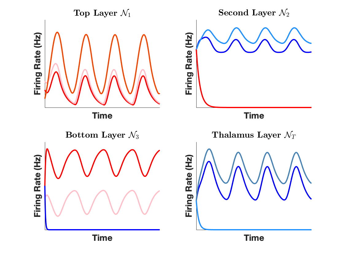
Figure 2: Trajectories of a three-layer hierarchical thalamocortical network under a periodic input. Red and blue lines correspond with excitatory and inhibitory nodes, resp. Each layer consists of three nodes with the top layer in the network containing only excitatory nodes, the thalamus being strictly inhibitory and layers two and three having both excitatory and inhibitory nodes. Using a control law designed through Theorem IV.4, in each layer other than the top layer, nodes are able to be either selectively inhibited to zero or recruited into a periodic equilibrium trajectory. Timescale ratios are $\epsilon_{2}=0.54$, $\epsilon_{3}=0.15$ and $\epsilon_{T}=0.61$.

Fig. 2 illustrates Theorem IV.4. While the result is proven for the case in which the thalamus has a timescale inside the hierarchy, it still holds when the thalamus timescale is at the top or bottom of the hierarchy. In these cases, the proof method remains the same, with the appropriate modifications to the inequalities derived in (23)-(28).

Remark IV.5.

(Comparison with strictly cortical networks): Regarding selective inhibition and recruitment, Theorem IV.4 is to multilayer thalamocortical networks what [20, Theorem IV.3] is to multilayer cortical networks. Despite the analytical similarities, the consideration of the thalamus provides a significant generalization from a biological perspective, as transthalamic connections exist in most brain networks [1]. From a technical viewpoint, the addition of the thalamus, while only adding a layer, significantly complicates the analysis due to its connection with all of the cortical layers. These connections result in every layer having connections from timescales not simply immediately above or below it in the hierarchy, which impacts the determination of convergence to equilibrium values for layers above the thalamus. Finally,the control laws (23)-(28) allow for smaller magnitude sufficient controls than for the strictly cortical networks determined in [20] due to the inhibitory properties of the thalamic connection matrices $\mathbf{W}_{i,T}$, cf Section VI. $\bullet$

V Star-connected Thalamocortical Networks

In this section we consider star-connected thalamocortical networks, cf. Fig. 1(b), where the cortical regions are each connected only to the thalamus and the dynamics are governed by (8)-(9). In this topology, there is no direct relationship between the timescales of each layer and as such, no hierarchical structure. Without timescale separation, the specifics of selective inhibition and recruitment, both in terms of equilibria and stability criteria, differ from the hierarchical case.

V-A Equilibria and Stability Conditions

With the lack of timescale separation, the decomposition described in Section IV-A of the network equilibrium map as a collection of equilibrium maps for each layer, with the state of layers higher in the hierarchy represented by a constant input, no longer holds. As such, equilibrium values must be determined concurrently for all the layers. Since the task-irrelevant components get selectively inhibited to zero, the equilibrium for the task-relevant components is given by the solution $\mathbf{x}_{i}^{1^{*}}$, $i\in\{1,\dots,N\}\cup\{T\}$ to the system of equations:

$$\mathbf{x}_{i}^{1} =[\mathbf{W}_{i,i}^{1,\mathrm{all}}\mathbf{x}_{i}+\mathbf{W}_{i,T}^{1,\mathrm{all}}\mathbf{x}_{T}+\mathbf{c}_{i}^{1}]_{\mathbf{0}}^{\mathbf{m}_{i}^{1}},\qquad i=1,\dots,N,$$

$$\mathbf{x}_{T}^{1} =[\mathbf{W}_{T}\mathbf{x}_{T}+\sum_{i=1}^{N}\mathbf{W}_{T,i}\mathbf{x}_{i}+\mathbf{c}_{T}^{1}]_{0}^{\mathbf{m}_{T}^{1}}.$$ (29)

The task-relevant equilibrium to which the system converges is dependent upon $\mathbf{c}_{i}\in\mathbb{R}^{n_{i}-r_{i}}$, $i\in\{1,\dots,N\}$ and $\mathbf{c}_{T}\in\mathbb{R}^{n_{T}-r_{T}}$, and so we represent it by $\mathbf{x}_{i}^{1^{*}}(\mathbf{c}_{1},\dots,\mathbf{c}_{N},\mathbf{c}_{T})$. In keeping with the role of layer $\mathcal{N}_{1}$ as driving the selective recruitment in the other layers, rather than being recruited itself, we consider in what follows an input signal $\mathbf{c}_{1}:\mathbb{R}_{\geq 0}\rightarrow\mathbb{R}^{n_{i}-r_{i}}$, rather than a constant, that gives rise to an equilibrium trajectory $\mathbf{x}_{i}^{1^{*}}(\mathbf{c}_{1}(t),\dots,\mathbf{c}_{N},\mathbf{c}_{T})$ for the dynamics.

As per the description of the star-connected thalamocortical network, cf Section III, only the task-irrelevant component of the dynamics is directly controlled, and as such the ability to achieve selective inhibition and recruitment is dependent on the stability properties of the task-relevant components. To ensure this, we employ below the fact [19, Theorem IV.8] that, for a generic linear-threshold network mode $\tau\dot{\mathbf{x}}=-\mathbf{x}+[\mathbf{W}\mathbf{x}+\mathbf{c}]_{\mathbf{0}}^{\mathbf{m}}$, the condition $\rho(|\mathbf{W}|)<1$ is sufficient to ensure that, for all $\mathbf{c}\in\mathbb{R}^{n}$, the dynamics is GES to an equilibrium.

V-B Selective Inhibition and Recruitment

We are ready to formalize selective inhibition and recruitment for star-connected networks and provide conditions for its achievement. We recall that the subnetwork $\mathcal{N}_{1}$ corresponds with a subcortical region applying a sensory input signal to the thalamus to be relayed to the cortical regions. As such, we do not inhibit any components in this subnetwork and instead assume that it is stable to a trajectory $\bar{\mathbf{x}}_{1}(\mathbf{c}_{1}(t))$ dictated by its own input signal. For the remaining layers, we wish to inhibit the task-irrelevant components to zero and recruit the task-relevant components to the equilibria trajectory $\mathbf{x}_{i}^{1^{*}}(\mathbf{c}_{1}(t),\dots,\mathbf{c}_{N},\mathbf{c}_{T})$, $i\in\{2,\dots,N\}\cup\{T\}$. This can be formalized to selective inhibition and recruitment is achieved if for the input layer $\mathcal{N}_{1}$,

[driving layer]: $$\quad\lim_{t\to\infty}\left\|\mathbf{x}_{1}(t)-\bar{\mathbf{x}}_{1}(\mathbf{c}_{1}(t))\right\|=0;$$ (30a)

and for all layers $$\{\mathcal{N}_{i}\}_{i=2}^{N} \mathcal{N}_{T}$$ and ,

[inhibition]: $$\quad\lim_{t\to\infty}\left\|\mathbf{x}_{i}^{0}(t)\right\|=0;$$ (30b)

[recruitment]: $$\quad\lim_{t\to\infty}\left\|\mathbf{x}_{i}^{1}(t)-\mathbf{x}_{i}^{1^{*}}(\mathbf{c}_{1}(t),\dots,\mathbf{c}_{N},\mathbf{c}_{T})\right\|=0.$$ (30c)

We also employ a weaker notion, referred to as $\epsilon$-selective inhibition and recruitment, which is met if there exists $t^{*}$ such that the functions in (30) are all upper bounded by $\epsilon>0$ for $t>t^{*}$. For convenience, we also introduce the notation:

$$\bar{\mathbf{W}}^{11} =\begin{bmatrix}\mathbf{W}_{1,1}&\mathbf{0}&\dots&\mathbf{0}&\mathbf{W}_{1,T}^{11}\\ \mathbf{0}&\mathbf{W}_{2,2}^{11}&\dots&\mathbf{0}&\mathbf{W}_{2,T}^{11}\\ \vdots&\dots&\ddots&\vdots&\vdots\\ \mathbf{0}&\mathbf{0}&\dots&\mathbf{W}_{N,N}^{11}&\mathbf{W}_{N,T}^{11}\\ \mathbf{W}_{T,1}^{11}&\mathbf{W}_{T,2}^{11}&\dots&\mathbf{W}_{T,N}^{11}&\mathbf{W}_{T}^{11}\end{bmatrix}.$$ (31)

Note the Schur decomposition $\bar{\mathbf{W}}^{11}=\mathbf{Q}^{\top}(\mathbf{D}_{\bar{\mathbf{W}}^{11}}+\mathbf{N}_{\bar{\mathbf{W}}^{11}})\mathbf{Q}$, where $\mathbf{Q}$ is unitary, $\mathbf{D}_{\bar{\mathbf{W}}^{11}}$ is diagonal, and $\mathbf{N}_{\bar{\mathbf{W}}^{11}}$ is upper triangular with a zero diagonal [33]. The next result establishes conditions to achieve selective inhibition and recruitment in star-connected systems without a hierarchy of timescales.

Theorem V.1.

(Selective inhibition and recruitment of star-connected networks): Consider an $N$-layer star-connected thalamocortical network as shown in Fig. 1(b), with layer dynamics given by (8) and (9). Suppose the following hold for all values of $\mathbf{c}_{i}\in\mathbb{R}^{n_{i}}$, $i\in\{1,\dots,N\}$, and $\mathbf{c}_{T}\in\mathbb{R}^{n_{T}}$:

1. The input layer $\mathcal{N}_{1}$ has no nodes to be inhibited, $\rho(|\mathbf{W}_{1,1}|)<1$, and the input $\mathbf{c}_{1}(t)$ lies in a compact set and has a bounded rate derivative;

2. For each $i\in\{2,\dots,N\}\cup\{T\}$, the matrix $\mathbf{W}_{i,i}^{11}$ satisfies $\rho(|\mathbf{W}_{i,i}^{11}|)\leq\alpha_{i}$, with $\alpha_{i}<1$;

3. If $\rho\big{(}\sum_{i=1}^{N}|\mathbf{W}_{i,T}^{11}\mathbf{W}_{T,i}^{11}|\big{)}\neq 0$, then $\alpha+\max(\delta,\delta^{1/p})<1$, where $p$ is the dimension of $\mathbf{N}_{\bar{\mathbf{W}}^{11}}$ and

   $$\alpha =\max_{i\in\{2,\dots,N\}\cup\{T\}}\{\alpha_{i}\},\qquad\delta=\gamma\sum_{j=1}^{p-1}\left\|\mathbf{N}_{\bar{\mathbf{W}}^{11}}\right\|^{j},$$

   $$\gamma =\max\{\sum_{i=1}^{N-1}\mathbf{W}_{i,T}^{11}\mathbf{W}_{i,T}^{11^{\top}},\sum_{i=1}^{N-1}\mathbf{W}_{T,i}^{11}\mathbf{W}_{T,i}^{11^{\top}}\}.$$

Then, there exist control laws $\mathbf{u}_{i}(t)=\mathbf{K}_{i}\mathbf{x}_{i}(t)+\bar{\mathbf{u}}_{i}(t)$, with $\mathbf{K}_{i}\in\mathbb{R}^{p_{i}\times n_{i}}$ and $\bar{\mathbf{u}}_{i}:\mathbb{R}_{\geq 0}\rightarrow\mathbb{R}_{\geq 0}^{p_{i}}$, and $\epsilon>0$ such that the cortical and thalamic regions within the closed-loop system achieve $\epsilon-$selective inhibition and recruitment. Furthermore, if $\left\|\dot{\mathbf{c}}_{1}(t)\right\|\to 0$ as $t\to\infty$, then the network achieves selective inhibition and recruitment (30).

Proof.

First, for cortical region $\mathcal{N}_{i}$, $i\in\{2,\dots,N\}$, define the control laws $\mathbf{u}_{i}(t)=\mathbf{B}_{i}\mathbf{K}_{i}\mathbf{x}_{i}(t)+\mathbf{B}_{i}\bar{\mathbf{u}}(t)$ such that

$$\mathbf{B}_{i}\mathbf{K}_{i} \leq-\mathbf{W}_{i,i}^{0,\mathrm{all}},$$ (32a)

$$\mathbf{B}_{i}\bar{\mathbf{u}}_{i}(t) \leq-\mathbf{W}_{i,T}^{0,\mathrm{all}}\mathbf{x}_{T}(t)-\mathbf{c}_{i}^{0}.$$ (32b)

In a similar fashion, define the control law for the thalamus, $\mathcal{N}_{T}$ by $\mathbf{u}_{T}(t)=\mathbf{B}_{T}\mathbf{K}_{T}\mathbf{x}_{T}(t)+\mathbf{B}_{T}\bar{\mathbf{u}}(t)$ such that it satisfies

$$\mathbf{B}_{T}\mathbf{K}_{T} \leq-\mathbf{W}_{T}^{0,\mathrm{all}},$$ (33a)

$$\mathbf{B}_{T}\bar{\mathbf{u}}_{T}(t) \leq-\mathbf{W}_{T,1}^{0,\mathrm{all}}\mathbf{x}_{1}(t)-\mathbf{c}_{T}^{0}.$$ (33b)

Now, we permute the system variables and define corresponding timescale matrices as follows

$$\bar{\mathbf{x}} =\begin{bmatrix}\mathbf{x}^{0}\\ \mathbf{x}^{1}\end{bmatrix}\qquad\mathbf{x}^{0}=\begin{bmatrix}\mathbf{x}_{2}^{0}&\dots&\mathbf{x}_{N}^{0}&\mathbf{x}_{T}^{0}\end{bmatrix}^{\top}$$

$$\mathbf{x}^{1} =\begin{bmatrix}\mathbf{x}_{1}&\mathbf{x}_{2}^{1}&\dots&\mathbf{x}_{N}^{1}&\mathbf{x}_{T}^{1}\end{bmatrix}^{\top}\qquad\tau^{0}=\text{diag}(\tau_{2},\dots,\tau_{N},\tau_{T})$$

$$\tau^{1} =\text{diag}(\tau_{1},\tau_{2},\dots,\tau_{N},\tau_{T}).$$

Substituting in the control laws (32) and (33), we have the following controlled system dynamics

$$\tau^{0}\dot{\mathbf{x}}^{0} =-\mathbf{x}^{0}$$ (34a)

$$\tau^{1}\dot{\mathbf{x}}^{1} =-\mathbf{x}^{1}+[\bar{\mathbf{W}}\bar{\mathbf{x}}+\mathbf{c}(t)]_{\mathbf{0}}^{\bar{\mathbf{m}}},$$ (34b)

where $\bar{\mathbf{W}}=\begin{bmatrix}\bar{\mathbf{W}}^{10}&\bar{\mathbf{W}}^{11}\end{bmatrix},$ with $\bar{\mathbf{W}}^{11}$ as in (31), and $\mathbf{c}(t)$ the permutation of the signal $\mathbf{c}_{1}(t)$ and the constants $\mathbf{c}_{i}$, $i\in\{2,\dots,N\}\cup\{T\}$ corresponding to the permuted variables. Now, we consider a ‘frozen’ version of the dynamics (34), in which we fix $\mathbf{c}_{1}(t)$ to a constant $\bar{\mathbf{c}}_{1}$. By [19, Lemma A.1] the frozen version of the dynamics (34) is GES to an equilibrium $\mathbf{x}^{*}$, with $\mathbf{x}^{0}\to\mathbf{0}$, if $\dot{\bf y}=-{\bf y}+[\bar{\mathbf{W}}^{11}{\bf y}+\mathbf{c}]_{\mathbf{0}}^{\bar{\mathbf{m}}}$ is GES to an equilibrium. By assumptions (ii) and (iii), along with [33, Theorem 2], we have that $\rho(\bar{\mathbf{W}}^{11})<1$ and therefore, the dynamics $\dot{\bf y}=-{\bf y}+[\bar{\mathbf{W}}^{11}{\bf y}+\mathbf{c}]_{\mathbf{0}}^{\bar{\mathbf{m}}}$ is GES to an equilibrium, cf. [19, Theorem IV.8]. Therefore the frozen version of (34) is GES to an equilibrium using the control laws defined above. Given this, we can apply the converse Lyapunov result given in Theorem .2 to get a Lyapunov function for the dynamics (34) that satisfies the requirements of Theorem .1. The direct application of this result then gives that selective inhibition and recruitment (30) is achieved if $\left\|\dot{\mathbf{c}}_{1}(t)\right\|\to 0$ and is $\epsilon$-selectively inhibited and recruited if it is bounded but does not tend to zero. ∎

Note that Theorem V.1 relies on the stability of the task-relevant dynamics of each network layer when considered independently and the assumption that the magnitude of the combination of thalamocortical and corticothalamic interconnections does not exceed a certain stability margin. The latter condition is consistent with neuroscientific observations: in fact, enhanced corticothalamic feedback may result in pathological behavior [34]. In particular, excessive corticothalamic feedback has been found to coincide with epileptic loss of consciousness in absence seizures due to over-inhibition in the cortical regions [35].

Remark V.2.

(Remote synchronization in star-connected brain networks): Remote synchronization is a phenomenon observed in the brain in which distant brain regions with similar structure synchronize their activity despite the lack of a direct link [36]. This should then naturally arise in star-connected networks if there is morphological symmetry between cortical regions, as this topology directly shows regions without direct links. From (V-A), we note that if any two cortical regions $\mathcal{N}_{i}$ and $\mathcal{N}_{j}$ have identical task-relevant dynamics, i.e., $\mathbf{W}_{i,i}^{1,\mathrm{all}}=\mathbf{W}_{j,j}^{1,\mathrm{all}}$, $\mathbf{W}_{i,T}^{1,\mathrm{all}}=\mathbf{W}_{j,T}^{1,\mathrm{all}}$ and $\mathbf{c}_{i}^{1}=\mathbf{c}_{j}^{1}$, it follows that the equilibrium points will satisfy $\mathbf{x}_{i}^{1^{*}}=\mathbf{x}_{j}^{1^{*}}$, meaning that remote synchronization is achieved provided that the conditions of Theorem V.1 are satisfied.

Remarkably, this conclusion seems to be independent of the particular dynamics of the individual layers. In fact, the work [37] studies remote synchronization in star-connected brain networks, cf. Fig. 1(b), with layer dynamics given by Kuramoto oscillator dynamics,

$$\dot{\theta}_{T} =\omega_{0}+\sum_{i=1}^{N}K_{i}\sin(\theta_{i}-\theta_{0}-\xi)$$

$$\dot{\theta}_{i} =\omega+A_{i}\sin(\theta_{0}-\theta_{i}-\xi),\qquad i=1,\dots,N.$$ (35)

According to [37], the outer cortical regions in star-connected brain networks can remotely synchronize despite no direct links between the regions provided the network dynamics satisfy conditions that parallel those required for the star-connected linear-threshold networks studied above. In particular, to be able to achieve remote synchronization, the network weights must satisfy $A_{i}\geq(N-1)K_{i}$ for all $i\in\{1,\dots,N\}$. This condition guarantees the existence of a locally stable equilibrium point, and is equivalent the requirement of the matrices defining the task-relevant components of the linear-threshold network being individually stable. $\bullet$

We conclude by noting that the thalamus, as a relay, can function as a failsafe for the hierarchical thalamocortical network, allowing for selective inhibition and recruitment even if corticocortical connections become damaged. In fact, observe that the hierarchical topology where the matrices $\mathbf{W}_{i,i-1},\mathbf{W}_{i,i+1}$ are equal to zero for all $i$ reduces to the star-connected topology, while maintaining the timescale separation between layers. Therefore, the star-connected topology with a hierarchical timescale structure can be considered as a failsafe for the hierarchical thalamocortical network. The next result provides conditions for selective inhibition and recruitment for this topology.

Corollary V.3.

(Selective inhibition of a star-connected hierarchical thalamocortical network): Consider a hierarchical star-connected thalamocortical network of the form shown in Fig. 1(b) with timescales $\tau_{1}\gg\tau_{2}\gg\dots\gg\tau_{N}$ and layer dynamics given by (5) and (7). Without loss of generality let $\tau_{T}$ be such that $\tau_{1}\gg\tau_{T}\gg\tau_{N}$ and let $a,b\in\{1,\dots,N\}$ such that $\tau_{a}\gg\tau_{T}\gg\tau_{b}$ and $b=a+1$. Assume the stability assumptions (17)-(21) for the reduced-order subnetworks are satisfied. Then, for $i\in\{1,\dots,N\}\cup\{T\}$ and constants $\mathbf{c}_{i}\in\mathbb{R}^{n_{i}}$ and $\mathbf{c}_{T}\in\mathbb{R}^{n_{T}}$, there exist control laws $\mathbf{u}_{i}(t)=\mathbf{K}_{i}\mathbf{x}_{i}(t)+\bar{\mathbf{u}_{i}}(t)$, with $\mathbf{K}_{i}\in\mathbb{R}^{p_{i}\times n_{i}}$ and $\bar{\mathbf{u}}_{i}:\mathbb{R}_{\geq 0}\rightarrow\mathbb{R}_{\geq 0}^{p_{i}}$, such that the closed-loop system achieves selective inhibition and recruitment (22).

The proof of the result is similar to that of Theorem IV.4, with differences occurring in the constructed control laws on the basis that $\mathbf{W}_{i,i+1}=\mathbf{W}_{i,i-1}=\mathbf{0}$ for all $i\in\{1,\dots,N\}$. The loss of these connections plays a significant role in the form of the control. In particular, the amount of feedforward control coming from the thalamus to the cortical regions increases, due to the fact that direct feedforward control between cortical regions is not possible. Fig. 3 illustrates Corollary V.3 on the star-connected network obtained by removing the direct connections between cortical regions in the network of Fig. 2.

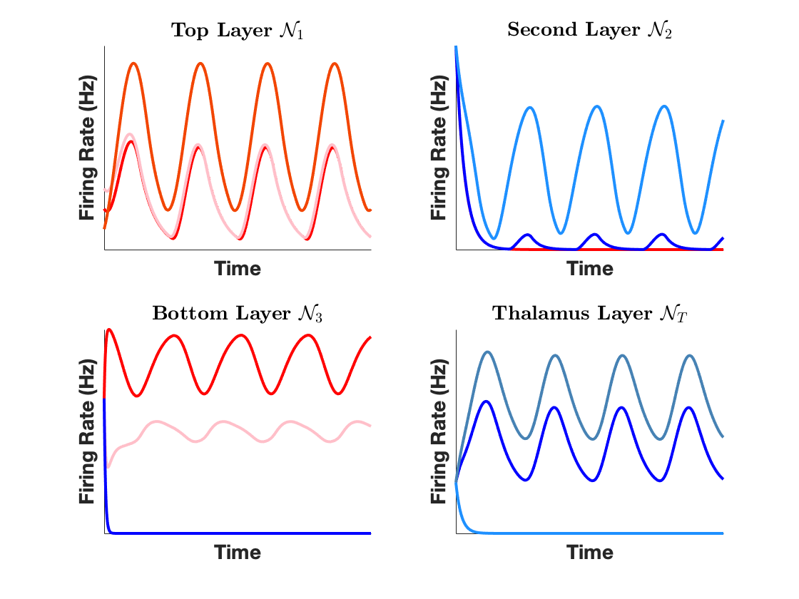
Figure 3: Trajectories of the network in Fig. 2 with the connections between the cortical regions removed. The star-connected topology allows for successful selective inhibition of the desired set of nodes despite the lack of connections between cortical regions (cf. Corollary V.3), providing a failsafe topology.

VI Quantitative Comparison of Cortical and Thalamocortical Networks

This section seeks to quantitatively illustrate ways in which the presence of the thalamus might have a beneficial effect in the behavior and performance of the dynamic models for brain networks adopted here. Fig. 3 has already illustrated the failsafe role played by the thalamus in hierarchical thalamocortical networks. Here we focus on two other beneficial impacts of the thalamus that we have observed in simulation: the required control magnitude to achieve selective inhibition and the convergence time in thalamocortical networks versus cortical ones.

Example VI.1.

(Reduced average control magnitude in thalamocortical vs cortical networks): We investigate the control magnitude required to achieve selective inhibition. Control magnitude here refers to the aggregate of the inputs at all layers integrated over time and averaged across trials. We consider hierarchical pairs of thalamocortical and cortical networks, where the latter is obtained by disconnecting the thalamus in the former. Fig. 4 shows that thalamocortical networks require a lower control magnitude to achieve selective inhibition in the cortical regions relative to the corresponding strictly cortical networks, matching the intuition that they are easier to selectively inhibit due to the thalamus impacting the cortical regions in an inhibitory fashion.

$\bullet$

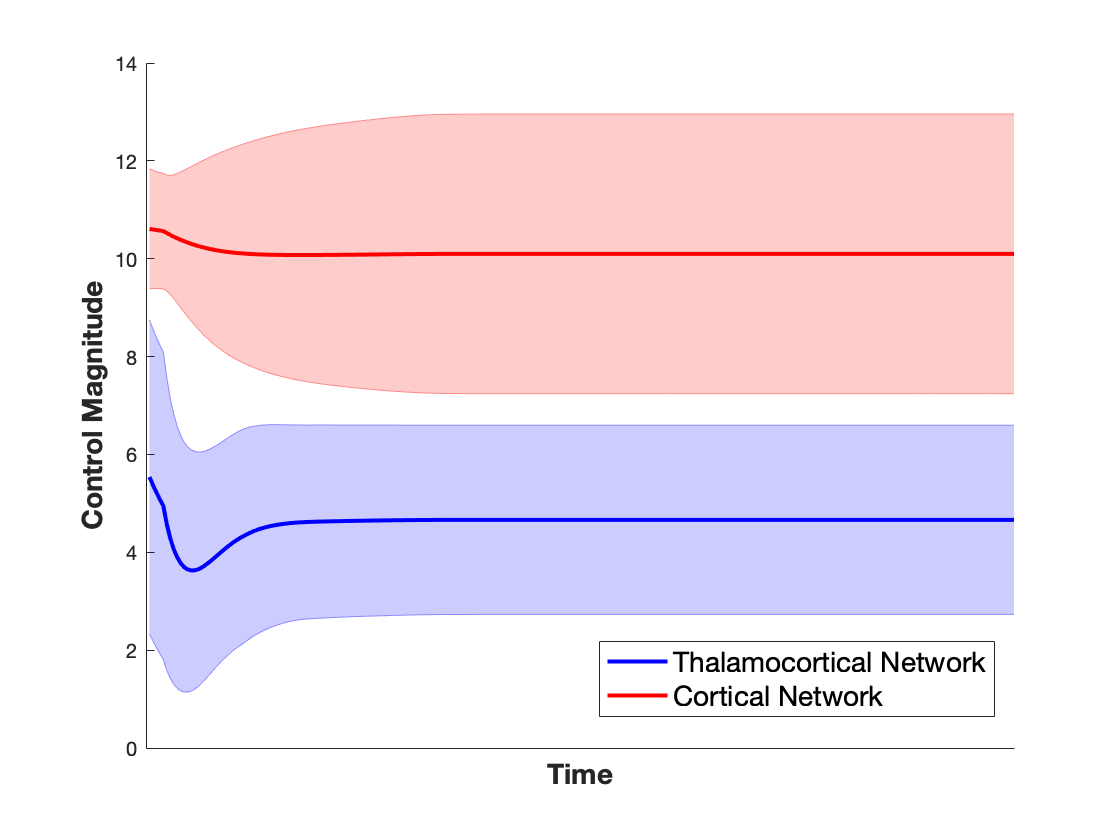
Figure 4: Comparison of average control magnitude in cortical and thalamocortical networks. The plot displays the control magnitude required to selectively inhibit the bottom cortical layer averaged over $100$ random thalamocortical networks and the corresponding cortical network in which the thalamus is removed. Shaded regions correspond to the error bars. All networks are composed of two three-node cortical regions. The top cortical layer has two excitatory nodes and the bottom layer has only one. The thalamus is composed of two inhibitory nodes. Each thalamocortical and cortical network generated satisfies the assumptions of Theorem IV.4 and [20, Theorem IV.3], resp., along with biological sign constraints. To make the required control magnitude directly comparable, the thalamocortical and cortical networks are inhibiting the same set of nodes within the bottom cortical layer.

Example VI.2.

(Convergence time of thalamocortical and cortical networks): Here we consider the speed at which thalamocortical networks converge to an equilibrium as another metric to evaluate the role of the thalamus. We compare the convergence time for a cortical network with that of a thalamocortical network maintaining the same cortical regions. While performing the comparison is interesting as a function of multiple network parameters (e.g., network size, layer size, ratio of excitatory-inhibitory nodes), we focus here specifically on the thalamus and, in particular, on varying its timescale with respect to the cortical regions in the model. Thalamocortical networks with varying timescales are of particular interest due to their existence in the brain, as even restricting only to the visual thalamus, the thalamus operates at both slow and fast timescales [38]. Fig. 5 shows that thalamocortical networks have faster average convergence time, with the margin between the two networks decreasing as the timescale $\tau_{T}$ increases. This validates the the beneficial role played by the thalamus, with faster thalamus dynamics (smaller $\tau_{T}$) helping the cortical regions converge faster, leading to overall decreased convergence time. $\bullet$

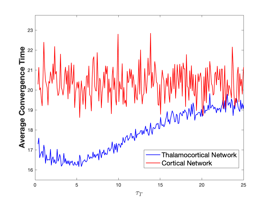
Figure 5: Convergence time of thalamocortical network with changing timescales. The graph illustrates the average convergence time to the equilibrium for $30$ randomly generated cortical and thalamocortical networks with $20$ layers, each containing two excitatory and two inhibitory nodes. For each simulation the initial condition is set to be a uniform distance away from the equilibrium and the set of nodes to be inhibited is randomly selected. The average convergence time for nodes within the thalamocortical network is lower than for the cortical network. As the timescale $\tau_{T}$ of the thalamus increases, the margin of improvement decreases.

VII Conclusions

We have studied the properties of both multilayer hierarchical and star-connected thalamocortical brain networks modeled with linear-threshold dynamics. Our primary motivation was understanding the role played by the thalamus in achieving selective inhibition and recruitment of neural populations. For both types of interconnection topologies, we have described how the equilibria at each layer depends on the rest of the network and identified suitable stability conditions. For hierarchical networks, these take the form of GES requirements of the reduced-order dynamics of individual layers. For star-connected thalamocortical network without a hierarchy of timescales, these take the form of stability of the task-relevant dynamics of each layer when considered independently and the magnitude of the combination of thalamocortical and corticothalamic interconnections not exceeding a certain stability margin. Future work will seek to analytically characterize the robustness and performance of thalamocortical networks, study the role of the thalamus in other cognitive tasks beyond selective attention (e.g., sleep and consciousness, oscillations, and learning), and explore the impact of the addition and deletion of neuronal populations (neurogenesis) in the performance and expressivity of brain networks.

Michael McCreesh received his B.A.Sc degree in Mathematics and Engineering and his M.A.Sc in Mathematics and Engineering from Queen’s University, Kingston, Canada in 2017 and 2019, resp. He is currently a Ph.D. student in the Department of Mechanical and Aerospace Engineering at the University of California San Diego. His current research interests include control theory and its application to theoretical neuroscience, in particular the application of dynamical systems to model brain networks.

Jorge Cortés (M’02, SM’06, F’14) received the Licenciatura degree in mathematics from Universidad de Zaragoza, Zaragoza, Spain, in 1997, and the Ph.D. degree in engineering mathematics from Universidad Carlos III de Madrid, Madrid, Spain, in 2001. He held postdoctoral positions with the University of Twente, Twente, The Netherlands, and the University of Illinois at Urbana-Champaign, Urbana, IL, USA. He was an Assistant Professor with the Department of Applied Mathematics and Statistics, University of California, Santa Cruz, CA, USA, from 2004 to 2007. He is currently a Professor in the Department of Mechanical and Aerospace Engineering, University of California, San Diego, CA, USA. He is the author of Geometric, Control and Numerical Aspects of Nonholonomic Systems (Springer-Verlag, 2002) and co-author (together with F. Bullo and S. Martínez) of Distributed Control of Robotic Networks (Princeton University Press, 2009). He is a Fellow of IEEE and SIAM. His current research interests include distributed control and optimization, network science, nonsmooth analysis, reasoning and decision making under uncertainty, network neuroscience, and multi-agent coordination in robotic, power, and transportation networks.

For completeness, here we include two results on the stability of slowly varying nonlinear systems to a continuum equilibria, generalized from [39, Theorem 3.1] to the case of exponential stability. Let

$$\dot{\mathbf{x}}=f(\mathbf{x}(t),\mathbf{d}(t)),$$ (36)

where $\mathbf{x}(t)\in\mathbb{R}^{n}$ and $\mathbf{d}(t)\in\mathcal{D}$, and $\mathcal{D}$ is a compact subset of $\mathbb{R}^{m}$. We assume $f$ is continuous on $\mathbb{R}^{n}\times\mathcal{D}$ and is locally Lipschitz in both $\mathbf{x}$ and $\mathbf{d}$. We further consider the ‘frozen’ version of the system (36) with a fixed parameter $\mathbf{d}$,

$$\dot{\mathbf{x}}=f(\mathbf{x}(t),\mathbf{d}),\quad\mathbf{d}\in\mathcal{D}.$$ (37)

We denote the solution to (37) for each initial condition $\mathbf{x}(t_{0})=\mathbf{x}_{0}$ and $\mathbf{d}\in\mathcal{D}$ by $\mathbf{x}(t,\mathbf{x}_{0},\mathbf{d})$. Let $\mathcal{A}$ be a forward invariant set of the system (37).

Theorem .1.

(Exponential Stability of Slowly Varying Nonlinear Systems): Consider the nonlinear system (36) and assume there exists a continuously differentiable function $V:\mathbb{R}^{n}\times\mathcal{D}\rightarrow\mathbb{R}$ such that

$$k_{1}|\mathbf{x}|_{\mathcal{A}}^{2} \leq V(\mathbf{x},\mathbf{d})\leq k_{2}|\mathbf{x}|_{\mathcal{A}}^{2}$$ (38a)

$$\frac{\partial V(\mathbf{x},\mathbf{d})}{\partial\mathbf{x}}f(\mathbf{x},\mathbf{d}) \leq-k_{3}|\mathbf{x}|_{\mathcal{A}}^{2}$$ (38b)

$$\left|\frac{\partial V(\mathbf{x},\mathbf{d})}{\partial\mathbf{d}}\right| \leq k,$$ (38c)

for all $\mathbf{x}\in\mathbb{R}^{n}$ and $\mathbf{d}\in\mathcal{D}$, with $k_{1},k_{2},k_{3}$ and $k$ nonnegative constants. If $\left\|\dot{d}(t)\right\|$ is uniformly bounded in time, then there exist constants $\gamma,\lambda$ and $T$ such that

$$|\mathbf{x}(t,\mathbf{x}_{0},\mathbf{d})|_{\mathcal{A}} \leq\gamma\left\|\mathbf{x}_{0}\right\|e^{-\lambda(t-t_{0})}\quad\forall~{}t_{0}\leq t\leq t_{0}+T$$ (39a)

$$|\mathbf{x}(t,\mathbf{x}_{0},\mathbf{d})|_{\mathcal{A}} \leq\frac{k_{3}}{k_{2}}|\mathbf{x}_{0}|_{\mathcal{A}}\quad\forall~{}t\geq t_{0},$$ (39b)

If $$\lim_{t\to\infty}\left\|\dot{\mathbf{d}}(t)\right\|=0$$, then the system is exponentially stable.

The proof follows a similar line of reasoning as in [39, Theorem 3.1] with slight modifications in the use of stability results from [40] to account for exponential stability. We now provide a converse Lyapunov result, modified from [39, Theorem 3.2], complementary to the above result.

Theorem .2.

(Converse Lyapunov Theorem for Slowly Varying Nonlinear Systems): If, for every fixed $\mathbf{d}\in\mathcal{D}$, the nonlinear system (36) is GES to an equilibrium, then there exists a Lyapunov function that satisfies (38a), (38b) and (38c).

The proof of this result is identical to [39, Theorem 3.2], with the assumption of GES giving the desired function form in the final step.

References

- [1] S. M. Sherman, “Thalamocortical interactions,” Current Opinion in Neurobiology, vol. 22, no. 4, pp. 575–579, 2012.
- [2] N. Tinbergen, “The hierarchical organization of nervous mechanisms underlying instinctive behaviour,” in Symposium for the Society for Experimental Biology, vol. 4, pp. 305–312, 1950.
- [3] A. R. Luria, “The functional organization of the brain,” Scientific American, vol. 222, no. 3, pp. 66–79, 1970.
- [4] S. J. Kiebel, J. Daunizeau, and K. J. Friston, “A hierarchy of time-scales and the brain,” PLOS Computational Biology, vol. 4, no. 11, p. e1000209, 2008.
- [5] J. D. Murray, A. Bernacchia, D. J. Freedman, R. Romo, J. D. Wallis, X. Cai, C. Padoa-Schioppa, T. Pasternak, H. Seo, D. Lee, and X. Wang, “A hierarchy of intrinsic timescales across primate cortex,” Nature Neuroscience, vol. 17, no. 12, p. 1661, 2014.
- [6] D. J. Felleman and D. C. V. Essen, “Distributed hierarchical processing in the primate cerebral cortex,” Cerebral Cortex, vol. 1, no. 1, pp. 1–47, 1991.
- [7] U. Hasson, J. Chen, and C. J. Honey, “Hierarchical process memory: memory as an integral component of information processing,” Trends in Cognitive Sciences, vol. 19, no. 6, pp. 304–313, 2015.
- [8] M. I. Rabinovich, I. Tristan, and P. Varona, “Hierarchical nonlinear dynamics of human attention,” Neuroscience & Biobehavioral Reviews, vol. 55, pp. 18–35, 2015.
- [9] K. Hwang, M. A. Bertolero, W. B. Liu, and M. D’Esposito, “The human thalamus is an integrative hub for functional brain networks,” Journal of Neuroscience, vol. 37, no. 23, pp. 5594–5607, 2017.
- [10] R. D. D’Souza and A. Burkhalter, “A laminar organization for selective cortico-cortical communication,” Frontiers in Neuroanatomy, vol. 11, p. 71, 2017.
- [11] M. M. Halassa and L. Acsády, “Thalamic inhibition: diverse sources, diverse scales,” Trends in Neurosciences, vol. 39, no. 10, pp. 680–693, 2016.
- [12] J. M. Alonso and H. A. Swadlow, “Thalamus controls recurrent cortical dynamics,” Nature Neuroscience, vol. 18, no. 12, pp. 1703–1704, 2015.
- [13] S. M. Sherman and R. W. Guillery, Exploring the Thalamus and Its Role in Cortical Function. MIT press, 2006.
- [14] L. Gabernet, S. P. Jadhav, D. E. Feldman, M. Carandini, and M. Scanziani, “Somatosensory integration controlled by dynamic thalamocortical feed-forward inhibition,” Neuron, vol. 48, no. 2, pp. 315–327, 2005.
- [15] S. Cruikshank, T. J. Lewis, and B. Connors, “Synaptic basis for intense thalamocortical activation of feedforward inhibitory cells in neocortex,” Nature Neuroscience, vol. 10, no. 4, pp. 462–468, 2007.
- [16] J. A. Harris, S. Mihalas, K. E. Hirokawa, J. D. Whitesell, H. Choi, A. Bernard, P. Bohn, S. Caldejon, L. Casal, A. Cho, et al., “Hierarchical organization of cortical and thalamic connectivity,” Nature, vol. 575, no. 7781, pp. 195–202, 2019.
- [17] R. Chaudhuri, K. Knoblauch, M. Gariel, H. Kennedy, and X. Wang, “A large-scale circuit mechanism for hierarchical dynamical processing in the primate cortex,” Neuron, vol. 88, no. 2, pp. 419–431, 2015.
- [18] K. Morrison, A. Degeratu, V. Itskov, and C. Curto, “Diversity of emergent dynamics in competitive threshold-linear networks: a preliminary report,” arXiv preprint arXiv:1605.04463, 2016.
- [19] E. Nozari and J. Cortés, “Hierarchical selective recruitment in linear-threshold brain networks. Part I: Intra-layer dynamics and selective inhibition,” IEEE Transactions on Automatic Control, vol. 66, no. 3, pp. 949–964, 2021.
- [20] E. Nozari and J. Cortés, “Hierarchical selective recruitment in linear-threshold brain networks. Part II: Inter-layer dynamics and top-down recruitment,” IEEE Transactions on Automatic Control, vol. 66, no. 3, pp. 965–980, 2021.
- [21] D. Liberzon, Switching in Systems and Control. Systems & Control: Foundations & Applications, Birkhäuser, 2003.
- [22] M. K. J. Johansson, Piecewise Linear Control Systems: A Computational Approach. Lecture Notes in Control and Information Sciences, Springer Berlin Heidelberg, 2003.
- [23] A. N. Tikhonov, “Systems of differential equations containing small parameters in the derivatives,” Matematicheskii Sbornik, vol. 73, no. 3, pp. 575–586, 1952.
- [24] P. V. Kokotović and H. K. Khalil, eds., Singular Perturbation Methods in Control: Analysis and Design. SIAM, 1999.
- [25] V. Veliov, “A generalization of the Tikhonov theorem for singularly perturbed differential inclusions,” Journal of Dynamical & Control Systems, vol. 3, no. 3, pp. 291–319, 1997.
- [26] P. Dayan and L. F. Abbott, Theoretical Neuroscience: Computational and Mathematical Modeling of Neural Systems. Computational Neuroscience, Cambridge, MA: MIT Press, 2001.
- [27] J. Chen, U. Hasson, and C. Honey, “Processing timescales as an organizing principle for primate cortex,” Neuron, vol. 88, no. 2, pp. 244–246, 2015.
- [28] S. M. Sherman and R. W. Guillery, “Distinct functions for direct and transthalamic corticocortical connections,” Journal of Neurophysiology, vol. 106, no. 3, pp. 1068–1077, 2011.
- [29] K. Reinhold, A. D. Lien, and M. Scanziani, “Distinct recurrent versus afferent dynamics in cortical visual processing,” Nature Neuroscience, vol. 18, no. 12, pp. 1789–1797, 2015.
- [30] A. S. Mitchell, S. M. Sherman, M. A. Sommer, R. G. Mair, R. P. Vertes, and Y. Chudasama, “Advances in understanding mechanisms of thalamic relays in cognition and behavior,” Journal of Neuroscience, vol. 34, no. 46, pp. 15340–15346, 2014.
- [31] F. Alcaraz, V. Fresno, A. R. Marchand, E. J. Kremer, E. Coutureau, and M. Wolff, “Thalamocortical and corticothalamic pathways differentially contribute to goal-directed behaviors in the rat,” Elife, vol. 7, p. e32517, 2018.
- [32] J. S. Isaacson and M. Scanziani, “How inhibition shapes cortical activity,” Neuron, vol. 72, no. 2, pp. 231–243, 2011.
- [33] K. E. Chu, “Generalization of the bauer-fike theorem,” Numerische Mathematik, vol. 49, no. 6, pp. 685–691, 1986.
- [34] K. George and J. M. Das, “Neuroanatomy, thalamocortical radiations,” StatPearls [Internet], 2020.
- [35] G. K. Kostopoulos, “Involvement of the thalamocortical system in epileptic loss of consciousness,” Epilepsia, vol. 42, pp. 13–19, 2001.
- [36] V. Vuksanović and P. Hövel, “Functional connectivity of distant cortical regions: role of remote synchronization and symmetry in interactions,” NeuroImage, vol. 97, pp. 1–8, 2014.
- [37] Y. Qin, Y. Kawano, and M. Cao, “Stability of remote synchronization in star networks of kuramoto oscillators,” in IEEE Conf. on Decision and Control, (Miami Beach, USA), pp. 5209–5214, 2018.
- [38] Z. Ye, X. Yu, C. M. Houston, Z. Aboukhalil, N. P. Franks, W. Wisden, and S. G. Brickley, “Fast and slow inhibition in the visual thalamus is influenced by allocating receptors with different subunits,” Frontiers in Cellular Neuroscience, vol. 11, p. 95, 2017.
- [39] S. Lee and H. Ahn, “Robust stability of slowly varying nonlinear systems having a continuum of equilibria,” in IEEE Conf. on Decision and Control, (Osaka, Japan), IEEE, Dec. 2015.
- [40] H. K. Khalil, Nonlinear Systems. Prentice Hall, 3 ed., 2002.