Deep Learning of DESI Mock Spectra to Find Damped Ly$\alpha$ Systems

Abstract

We have updated and applied a convolutional neural network (CNN) machine learning model to discover and characterize damped Ly$\alpha$ systems (DLAs) based on Dark Energy Spectroscopic Instrument (DESI) mock spectra. We have optimized the training process and constructed a CNN model that yields a DLA classification accuracy above 99$\%$ for spectra which have signal-to-noise (S/N) above 5 per pixel. Classification accuracy is the rate of correct classifications. This accuracy remains above 97$\%$ for lower signal-to-noise (S/N) $\approx 1$ spectra. This CNN model provides estimations for redshift and HI column density with standard deviations of 0.002 and 0.17 dex for spectra with S/N above 3 per pixel. Also, this DLA finder is able to identify overlapping DLAs and sub-DLAs. Further, the impact of different DLA catalogs on the measurement of Baryon Acoustic Oscillation (BAO) is investigated. The cosmological fitting parameter result for BAO has less than $0.61\%$ difference compared to analysis of the mock results with perfect knowledge of DLAs. This difference is lower than the statistical error for the first year estimated from the mock spectra: above $1.7\%$. We also compared the performance of CNN and Gaussian Process (GP) model. Our improved CNN model has moderately 14$\%$ higher purity and 7$\%$ higher completeness than an older version of GP code, for S/N $>$ 3. Both codes provide good DLA redshift estimates, but the GP produces a better column density estimate by $24\%$ less standard deviation. A credible DLA catalog for DESI main survey can be provided by combining these two algorithms.

1 Introduction

The absorption systems in the spectra of the quasi-stellar-objects (QSOs) are widely used to probe the properties of the early universe (e.g., Rauch, 1998; Wolfe et al., 1986). Using QSO absorption line systems (e.g., Ly$\alpha$ and metal lines), one can probe a wide range of scales, including the gas properties inside and around galaxies (e.g., Fumagalli et al., 2011). Further, the QSO absorption line systems are used to reconstruct the cosmic web on a few tens of Mpc (e.g., McDonald, 2003; Cai et al., 2016; Lee et al., 2014; Cai et al., 2017; Li et al., 2021), and test cosmological models on the cosmological scale of hundreds of Mpc (e.g., Pérez-Ràfols et al., 2018). Among the absorption systems, damped Ly$\alpha$ systems (DLAs) are a population of strong absorbers with integrated neutral hydrogen (HI) column densities $N_{\rm{HI}}$ $>$ $2\times 10^{20}$ cm^-2 (e.g., Wolfe et al., 2005). DLAs serve as the dominant reservoirs of atomic hydrogen in the universe and offer a unique opportunity to probe the early universe (e.g., Prochaska & Wolfe, 1997; Zafar et al., 2013). Their absorption can be described using the Voigt profile which fits the damping wings driven by the natural broadening of the Ly$\alpha$ transition(e.g., Lee et al., 2020). Recently, DLAs are widely used to probe the circumgalactic medium (CGM) around galaxies, especially high-redshift galaxies at $z>2$ (e.g., Noterdaeme et al., 2019; Gardner et al., 1997). Simulations show that the majority of gas which gives rise to DLAs is associated with galaxies (e.g., Bird et al., 2014; Grudić et al., 2020; Rahmati et al., 2014). A complete understanding of galaxy evolution is based on the analysis for the properties of neutral gas(e.g., Krogager et al., 2020). Besides, a large sample of QSOs and DLAs can be used for measuring a variety of cross-correlations and auto-correlations, and this could help to fit the Baryon Acoustic Oscillation (BAO) at $z>2$.

Previously, with the help from visual inspection, Prochaska & Herbert-Fort (2004); Prochaska et al. (2005) searched for DLA candidates in SDSS spectra by running a window along the spectra to identify the DLA trough as a region where the signal-to-noise ratio (S/N) is significantly lower than the characteristic S/N in the vicinity. Later, by utilizing a fully automatic procedure based on classical statistics, Noterdaeme et al. (2009, 2012a) identified DLAs in SDSS/DR7 and SDSS-III/BOSS survey. Further, with the rapid increase of the spectral data in the era of eBOSS and future surveys, the efficient and accurate detection of DLAs from low S/N spectra is becoming a technical challenge. An automated technique using Gaussian Process is applied to detect DLAs along QSO sightlines(Garnett et al., 2017; Ho et al., 2020). Recently, in Parks et al. (2018), a Convolutional Neural Networks (CNN) model was designed to detect and characterize DLAs in the QSO spectra of the SDSS and BOSS survey. This algorithm yields a classification accuracy of 99$\%$ on spectra with S/N above five. The classification accuracy is defined as the proportion of results with correct predictions. The estimation for column densities and redshifts both have median values consistent with the ground truth, with a scattering of standard deviation of column density of $\sigma(logN_{\rm{HI}})$=0.15 and redshift of $\sigma(z)$=0.002, respectively. This CNN model is also applied to SDSS DR16 and a DLA catalog is generated by this algorithm Chabanier et al. (2021).

DESI (Dark Energy Spectroscopic Instrument) is a stage IV spectroscopic survey project, and it is a 5-year survey for galaxies, QSOs and Milky Way stars, covering 14,000 deg² DESI Collaboration et al. (2016a). The highest redshift coverage of DESI comes from QSOs. At higher redshift, DESI will use QSOs as backlights to measure clustering in the Ly$\alpha$ forest, the series of HI absorption lines in the spectra of distant QSOs. These absorption lines are produced by the Ly$\alpha$ electron transition of the neutral hydrogen Liske et al. (1998). About 2.4 million QSO spectra are expected to be produced Yèche et al. (2020), tracing the 3D distribution of the intergalactic gas at $z\gtrsim 2$ with a survey volume of 3 Gpc³. Comparing with the SDSS survey, it increases the Ly$\alpha$ forest survey volume by an order of magnitude. The Ly$\alpha$ forest is now used to provide the BAO measurement at $z\gtrsim 2$. du Mas des Bourboux et al. (2020) show that the forest with identified DLAs has to be specially treated when BAO analysis is conducted. DLAs will reduce the flux transmission field for the correlation estimate. The spectra pixels where a DLA reduces the transmission by more than 20$\%$ should not be used because these pixels will cause a bias in the final BAO measurement. That makes a DLA catalog indispensable for precise and accurate BAO fitting analysis.

Our paper aims to develop a DLA finder for the DESI survey. The method adopted is based on the CNN model (Parks et al., 2018), and we improve the CNN model using DESI mock spectra. Different DESI mock spectra were chosen to make this algorithm available for a wide range of S/N levels. The minimum S/N of the mock spectra which we used is 0.31. We have updated the framework to TensorFlow2.0. Our neural network was trained on a server with two NVIDIA Tesla V100 GPUs. After developing the CNN model, we use it to get the DLA catalog for the DESI mock spectra. We have also conducted BAO analysis tests to examine the effects of different DLA catalogs with different definitions.

This paper is organized as follows. In Section 2, we introduce the basic physical features of damping wings and the mock spectra for this paper. In Section 3, the description of the training process is present, including dataset generation, label setting, and training process. Model validation is discussed in Section 4. The comparison of CNN model and Gaussian Process (GP) model (Ho et al., 2020) on detecting DLAs is discussed in Section 5. In Section 6, the DLA catalog is generated. Further, the comparison of BAO fitting results using our DLA catalog and mock catalog is quantified. All codes related are available at https://github.com/cosmodesi/desi-dlas

2 DLA survey

2.1 Basic Terminology of DLA

Among all the Ly$\alpha$ absorbers, DLAs have the highest HI column densities of $N_{\rm{HI}}\geq 2\times 10^{20}\rm{cm}^{-2}$. At lower column densities, we designate absorption systems with $10^{17}\rm{cm}^{-2}\leq N_{\rm{HI}}\leq 2\times 10^{20}\rm{cm}^{-2}$ as Ly$\alpha$ limit systems (LLSs) including sub-DLAs with $10^{19}\rm{cm}^{-2}\leq N_{\rm{HI}}\leq 2\times 10^{20}\rm{cm}^{-2}$ or so-called super Lyman limit systems (SLLSs) (e.g., Péroux et al., 2003; Prochaska et al., 2015). At even lower column densities, these systems are called Ly$\alpha$ forest absorbers with $N_{\rm{HI}}\leq 10^{17}\rm{cm}^{-2}$, corresponding to the intergalactic hydrogen “clouds” along the QSO sightline (e.g., McQuinn, 2016). The fundamental difference between DLAs and other Ly$\alpha$ absorbers is that hydrogen is mainly neutral in DLAs, while in all other absorption systems it is ionized (e.g., Wolfe et al., 2005).

DLAs can be fitted by the Voigt profile, which is the convolution of Lorentz profile and Gaussian profile (Draine, 2011). According to the Uncertainty Principle, the energy level of an electron has a finite width. Therefore when an electron transitions between different energy levels, the corresponding frequency also has a certain range of distribution. This broadening is called natural broadening and it can be described by a Lorentz profile. Meanwhile, the Doppler effect causes Doppler broadening, which is fitted by a Gaussian profile when the gas satisfies a Maxwellian velocity distribution. The broadening of Ly$\alpha$ absorption lines is mainly caused by natural broadening and Doppler broadening (e.g., Lee et al., 2020).

At higher column densities, absorbers become optically thicker, and the Voigt profile can be characterized by a dark trough and the Lorentz damping wing, making it possible to identify individual absorbers from even a moderate S/N spectrum.

2.2 DESI Mock Spectra

2.2.1 Data Sample

The DESI mock spectra are representative of the data quality (e.g., S/N, resolution) of DESI real data. The location of DLAs and their column density are known in mock spectra, so the mock spectra can be used to train the CNN model and evaluate its performance. We choose four mock spectral database (mocks) from LyaCoLoRe mocks generated by the DESI Ly$\alpha$ Forest Working Group (Farr et al., 2020). To add DLAs in the mock spectra, the location of DLAs can be derived by a Gaussian field which is used to compute the density and velocities in the spectra (Font-Ribera & Miralda-Escudé, 2012). Then a column density is allocated to each DLA following the observed column density distribution from pyigm , and the absorption profile is calculated using a Voigt template. After these steps are done in the LyaCoLoRe mock production stage (Farr et al., 2020), DLAs can be inserted into the final synthetic spectra. Table 1 lists the information of the four mock database we used.

Table 1: Information of four DESI Mock

Name	Exposure Time	DLAs	Metals	BALs
	(1000s)
desi-0.2-100	100	Y	Y	N
desi-0.2-4	4	Y	Y	N
desi-0.2-1	1	Y	Y	N
desiY1-0.2-DLA	multiple	Y	N	N

The first three mocks have the same QSO catalog with different exposure times. The redshift of QSOs in the mock catalog is from 1.8 to 3.8. The continuum of these QSOs are generated using the publicly available package simqso as implemented in desisim code . The basic procedure is to generate an unabsorbed continuum for each QSO by adding a set of emission lines on top of a broken power law continuum model. The simqso is based on McGreer et al. (2013), however for these DESI mocks the emission lines had been tuned to provide a similar mean continuum, in the Lyman-$\alpha$ and Lyman-$\beta$ forest region, to that observed in eBOSS DR16 (du Mas des Bourboux et al., 2020). A wider description of the desisim implementation to generate the continuum, as well as the full synthetic spectra production itself, including the DLA insertion, will be presented in detail in Gonzalez-Morales & DESI Lyman $\alpha$ Working Group (In preparation) ; it is worth noticing that eBOSS DR16 used a quite similar mock set. There are many different versions of mock spectra in DESI, we choose some versions that the mock spectra are inserted with DLAs to do the training. For the spectra we used, the marked number ’0.2’ means that these spectra are inserted with DLAs. The last marked number (such as ’100’, ’4’, ’1’) stands for the exposure time these mock spectra have. The mock spectra ’desi-0.2-100’ have the S/N level equal to the spectra with exposure time $10^{5}$s. This is the most noise free sample in our paper. For ’desi-0.2-1’ and ’desi-0.2-4’ mocks, simulated QSO spectra have a fixed S/N level similar to DESI spectra observed one or four DESI effective times, 1000s and 4000s respectively.

The last mock, DesiY1-0.2-DLA is more realistic of what we would expect from the DESI first year observations, since those were constructed using a survey simulation to determine what region of the DESI footprint (Dey et al., 2019) would be covered during DESI’s first year, given a random realization of observing conditions. Such survey simulation also includes a similar target selection criteria as the main DESI Survey and a simplified fiber assign procedure to reflect that high redshift QSO can be observed up to four times (of  1000s each), as opposed to most target that are observed only once, depending on what other targets are available to be observed and whether we know the QSO redshift with high significance. This procedure results in a mock spectra sample of low redshift and high redshift QSOs which have a distribution of exposure times ranging from 1000s to 4000s, i.e it has a more realistic S/N distribution. These simulations were done using several pieces of desicode and were presented in Herrera-Alcantar (2020).

The BAL (broad absorption lines) features have similar profile to DLAs. We do not simulate BAL features in all the mock we used. This is to avoid their confusion on the training and reducing false-positive predictions of the model.

2.2.2 Data Structure of DESI Spectra

The DESI spectrometer uses three cameras to measure the flux in different wavelength channels. Every spectrum in the same camera shares the same wavelength array. The three channels are given in Table 2.

We used a class named DesiMock to store the various information of every spectrum. As shown in Figure 1, using the spectrum TARGETID as the index, each spectrum contains flux, error array, celestial coordinates, QSO redshift, S/N, and the DLA information, which contains the DLA ID, DLA central wavelength, and neutral hydrogen column density ($N_{\rm{HI}}$). We read the spectral data from this DesiMock class.

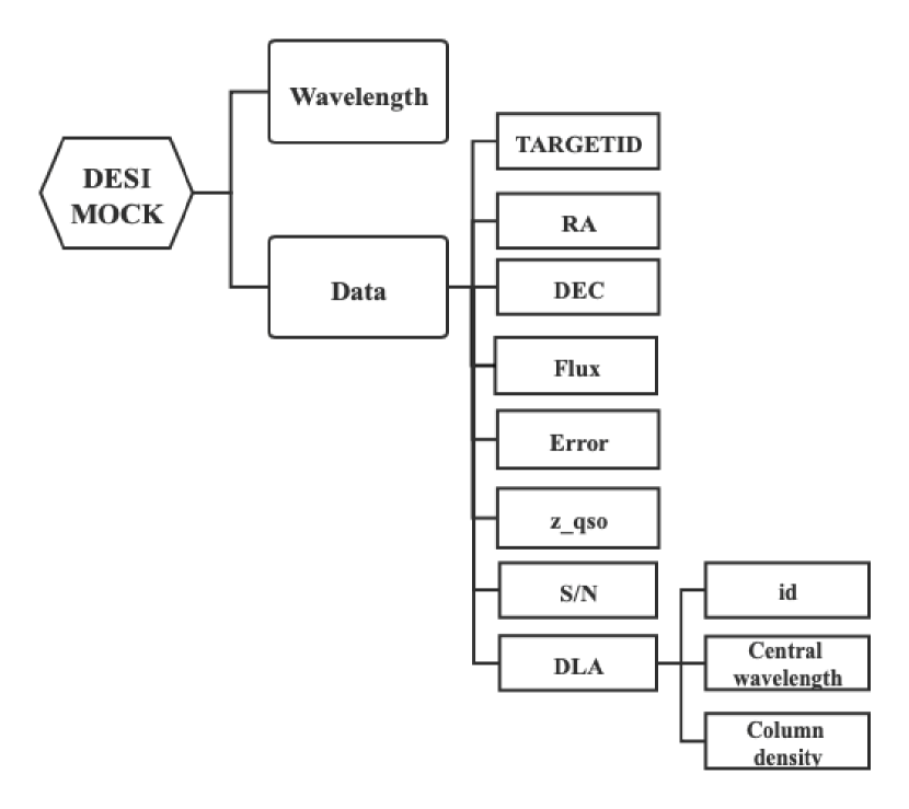
Figure 1: In the data structure of the DESIMOCK class, the wavelength array and the information of every spectrum are stored separately, including TARGETID, RA, DEC, etc.

2.2.3 S/N Definition

Figure 2 shows three spectra with different S/N of the same QSO (Mock spectrum ID: 170257611) with emission redshift $z_{em}\approx 3.395$. The S/N of the spectra in Figure 2 is estimated from the median flux of the data to the error array. Note the QSO rest-frame 1420Å to 1480Å do not have strong line features, and thus, we define the S/N of each mock spectrum as follows:

$$\rm{S/N}_{\rm{sightline}}=\rm{median}\left(\frac{{\rm flux(\lambda)}}{{\rm error(\lambda)}}\right),\ \lambda=1420-1480\rm{\AA}$$ (1)

The S/N definition is for per pixel. The following S/N values in this paper are all per pixel. Note that the S/N of the Ly $\alpha$ forest is much lower than the S/N defined here. For example, for a spectrum with S/N $=$ 3, the typical S/N in the forest region could be lower than unity.

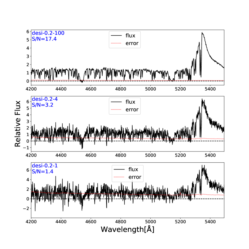
Figure 2: The three mock spectra of a QSO at $z_{em}\approx 3.395$ which exhibits two DLAs at $z_{\rm{abs}}\approx 2.733,3.330$ with $N_{\rm{HI}}\approx 10^{20.69}\rm{cm^{-2}},10^{20.23}\rm{cm^{-2}}$, which can be seen on the graph at the wavelength $\lambda_{\rm{abs}}\approx 4538\rm{\AA},5142\rm{\AA}$ respectively. The signal-to-noise (S/N) is shown at the upper left of each panel. The black line is the flux and the red dashed line is error.

Figure 3 displays the S/N distribution of the four mock datasets. The spectra used for training and prediction should have similar S/N ratios. Therefore, we used the first three mocks to train models for each mock respectively, as described in Section 3. The last mock desiY1-0.2-DLA is used to validate the three models, as described in Section 4.

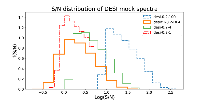
Figure 3: S/N distribution of four mocks. The three different mocks: desi-0.2-100, desi-0.2-4, desi-0.2-1 are used to train the CNN model at different S/N. It can be seen that the mock desiY1-0.2-DLA has more spectra with S/N$<$1.

3 Training

3.1 Preprocessing

3.1.1 Rebin

Spectral rebin consists of changing the size of the spectral bins of each spectra depending on the width of the line (Jolly et al., 2020). The dispersion $\Delta\lambda$ of the DESI mock spectra is $\approx 0.8\rm{\AA}$ per pixel, and hence the resolution is not a constant along the spectrum ($R=\frac{\lambda}{\Delta\lambda}$). The instruments for DESI cover wavelength range from 360nm to 980nm with resolution R=2000–5500 depending on wavelength(DESI Collaboration et al., 2016b). This means that in the DESI spectra, the number of pixels that span a DLA feature with a given $N_{\rm{HI}}$ is proportional to their redshift. A DLA at higher redshift has more pixel numbers than a DLA with same column density but at lower redshift. This will affect the model estimation of the HI column density. To correct this effect, we have to make sure the pixel size is a constant in the velocity-space. Thus, we set:

$$\frac{\Delta\lambda}{\lambda}=ln(1+\frac{\Delta v}{c})$$ (2)

where the $\Delta\lambda$ represents the dispersion per pixel, and $\Delta v$ represents the median pixel size in velocity. Then, we interpolate the original grid to the rebinned new grid with the pixel size equal to $\Delta v/c$. As seen in Table 2, we set the pixel size as the median velocity value in each channel.

Table 2: Value of resolution for three channels

Channel	Blue Channel	Red Channel	Z Channel
Wavelength($\rm\AA$)	3570-5950	5625-7740	7435-9833
$\Delta$ v (km/s)	63.0	44.9	34.7

3.1.2 Generating Datasets for Training and Validation

Previous DLA surveys (Noterdaeme et al., 2009) firstly estimate the QSO continua and then normalize the flux. Nevertheless, Parks et al. (2018) claimed that CNN learned to account for the continuum during the training. The CNN model could potentially detect DLAs without modeling the QSO continuum. Thus, we only use the median flux in the interval of 1420Å to 1480Å to do the normalization. Then, we construct the appropriate flux dataset for training and validation. The sightlines are processed in the following paragraphs. Similar treatment can be found in Parks et al. (2018).

• We only use a fixed range of the sightline ranging from 900 Å to 1346 Å in the QSO rest frame. The lower bound ensures that intervening optically thick HI gas below 900Å does not affect the identification of DLAs, and the upper bound ensures that DLAs on or near the QSO Ly$\alpha$ emission can be recovered. The purpose of choosing 1346 as an upper limit is to avoid missing some high column density associated DLAs which can blocks the Broad Line Region emission from the QSOs Finley et al. (2013) (for example, DLAs with $N_{\rm{HI}}>10^{22}$ and less than 1500$kms^{-1}$ from the QSOs redshift). Among more than 40000 DLA candidates detected by CNN in desiY1-0.2-DLA mock spectra, only 79 DLAs are located above the rest-frame 1216Å, and they can be excluded using the redshift cut.

• Each spectrum contains more than 2000 pixels. Inputting the whole sightline directly into the model leads to difficulties in discriminating multiple DLAs. Thus, we input a sliding window of a fixed pixel regions centered on each pixel into the model. The choice of window size and the hyperparameter selection process are discussed in detail in Section 3.3.

• Since there are far more regions without DLAs than regions with DLAs, our training sets maintain a 50/50 balance between training on positive and negative regions. This means the training datasets have half regions with DLAs and half regions without DLAs. This can help to train the CNN model on both positive and negative samples.

• Some regions of spectra are not included in the datasets. In the training set, we exclude the fixed pixels regions centered on DLA boundary and Ly$\beta$ absorption regions. 60 pixels on DLA boundary are avoided in the training set. We mask 15$\AA$ region around the Ly$\beta$ absorption. When we label the dataset, the classification value changes abruptly from 1 to 0 on the DLA boundary, which confuse the model. The Ly$\beta$ absorption lines corresponding to DLAs may be incorrectly detected as DLAs coming from the lower redshift.

• Flatten the column density distribution of SLLSs and DLAs. The dashed line of Figure 4 shows the $N_{\rm{HI}}$ distribution of the mixed mock spectra. The mixed spectral database is combined with different DESI mock catalogs including desi-0.2-100, desi-0.2-4 and desi-0.2-1. There are far more low $N_{\rm{HI}}$ DLAs than high $N_{\rm{HI}}$ DLAs which would induce bias towards to lower value when estimating column density in the algorithm. Thus, we manually inserted DLAs and super Lyman limit systems (SLLSs) into sightlines without high column density systems (HCDs), following the method described in Section 4.2 of Parks et al. (2018). The redshift distribution for the inserted DLAs is uniformed to avoid bias in training. The final $N_{\rm{HI}}$ distribution of our training sets is uniform with log $N_{\rm{HI}}$ ranging from 19.3 to 22.5 for multiple exposure time mocks (desi-0.2-100 and desi-0.2-4) and from 20.0 to 22.5 for single exposure time mock (desi-0.2-1), shown in the solid line of Figure 4. If we do not make the log $N_{\rm{HI}}$ uniformed, the CNN model will perform a bias for $N_{\rm{HI}}$ estimate. The $N_{\rm{HI}}$ distribution for training is uniformed to avoid the bias.

Following these procedures, we generate DLA training samples.

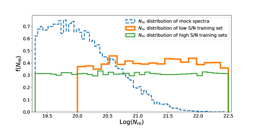
Figure 4: $N_{\rm{HI}}$ distribution of mock spectra and training sets. There are more DLAs with low column density in the mock data which follows the empirically measured distribution. The distribution of column density in training data is uniformed to reduce bias of the model to lower $N_{\rm HI}$ values.

In Table 3, we list the number of sightlines containing different absorbers for the training sets. With the same distribution as training sets, we generated the validation sets for Section 4, see Table 4.

Table 3: Information of Training Sets

S/N Level	DLAS	high $N_{\rm{HI}}$ DLAs	total number of sightlines	total number of absorbers	mock name
S/N 1-3	50893	34128	45748	57970	desi-0.2-1
S/N 3-6	48068	17099	100000	127347	desi-0.2-4
S/N 6-	58453	39453	65369	85436	desi-0.2-100

Table 4: Information of Validation Sets

S/N Level	DLAS	high $N_{\rm{HI}}$ DLAs	total number of sightlines	total number of absorbers	mock name
S/N 1-3	5366	3657	4938	6040	desi-0.2-1
S/N 3-6	20365	7267	43224	55166	desi-0.2-4
S/N 6-	6539	1360	47424	19917	desi-0.2-100

3.1.3 Improvement on Low S/N spectra

More than $70\%$ of the mock spectra have S/N$<$3. The classification accuracy for these low S/N spectra is only $93\%$ using the initial model. To improve the accuracy, we used the median smoothing method to optimize the preprocessing. Smoothing spectra reduces the resolution but it improves the S/N level. Accordingly, for dealing with low S/N spectra, we set the training data as a two dimensional array ($600\times 4$). The first row is the original flux. The other three rows are the median smoothing results for 3 pixels, 7 pixels, and 15 pixels. The CNN model is adjusted according to this new training data. The smoothing process and result are shown in Figure 5.

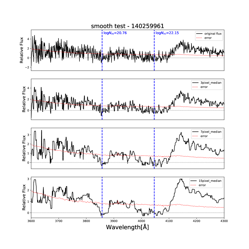
Figure 5: Smoothing result for the spectra. The blue dashed line stands for the center of DLAs. The red dashed line is the error for the spectra. The upper panel is the original flux. The lower three panels show the flux after median smoothing for 3 pixels, 7 pixels, and 15 pixels.

3.2 CNN Structure and Model Training

We followed the standard CNN architecture constructed in Parks et al. (2018). As shown in Figure 6, this model has three convolutional layers, each with a max pooling layer, following a fully connected layer and the last layer containing three separate fully connected sub-layers.

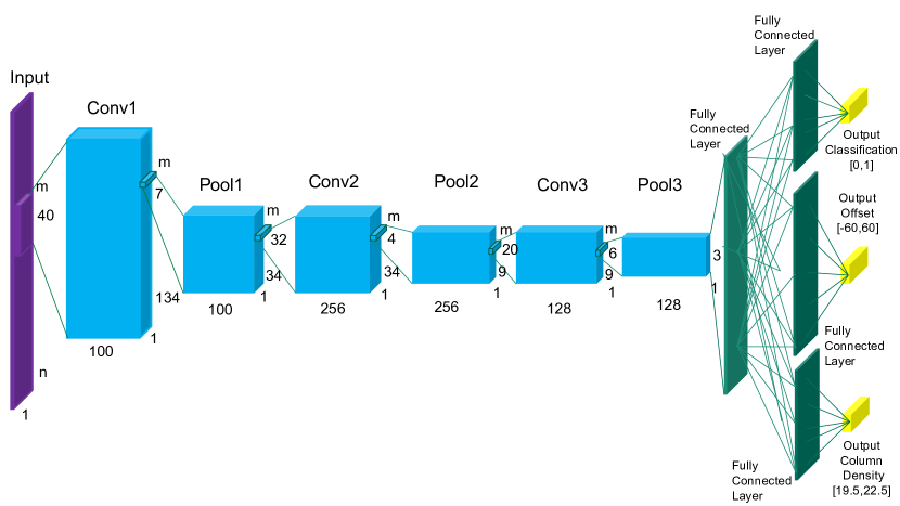
Figure 6: The standard CNN architecture we used, casting DLAs as a 1D image problem. There are three convolutional layers, three pooling layers, one fully connected layers, and three sub-fully connected layers. We have reset two parameters variable. One is $n$, it stands for how many pixels one window contains, it could be 400 or 600. The other one is $m$, it means the dimensions of the input data, the value of it is 1 or 4 (median smoothing for low S/N spectra). The three sub-fully connected layers are correspond to three labels: classification, offset and column density.

We trained our model for $10^{6}$ iterations each time. During the training process, we recorded the training accuracy every 200 steps and testing accuracy every 5000 steps. The classification accuracy improves more than 90$\%$ at the first $10^{5}$ steps. But it achieves the best accuracy of 99$\%$ (for S/N$>5$ spectra, spectra with different S/N levels have different best accuracy) at about $8\times 10^{5}$ steps. Then, the accuracy improves less than $0.001\%$ for the rest of the steps. Thus, $10^{6}$ iterations are enough for this training. The final classification accuracy for different S/N spectra are shown in Table 5. The training accuracy is the classification accuracy during training, and the definition of testing accuracy is similar. After the smoothing adjustments, the classification accuracy rises from 93$\%$ to 97$\%$ for spectra with S/N$<$3.

Table 5: Training and Testing Accuracy

S/N Level	Training Accuracy	Testing Accuracy
S/N $>$6	99$\%$	99$\%$
S/N 3-6	98$\%$	97$\%$
S/N 1-3	94$\%$	93$\%$
S/N 1-3(smooth)	97$\%$	97$\%$

The definition of classification accuracy is based on the confusion matrix Table 6. The label in this confusion matrix is the ’pred’ label as described in Section 3.2. The classification accuracy is defined as follows:

Table 6: Confusion Matrix

Label	GroundTruth 0	GroundTruth 1
Prediction 0	True Negative (TN)	False Negative (FN)
Prediction 1	False Positive (FP)	True Positive (TP)

$$Accuracy=\frac{TP+TN}{TP+FP+TN+FN}$$ (3)

This model yields four outputs for every window of the spectrum, three labels from the full connected layers as shown in Figure 6 and the confidence level:

1. ’Prediction’, labeled as ’pred’ in the code. This is the classification of the DLA. The value of this label is 0.0 or 1.0 . 1.0 stands for that the model detects a DLA in this window and 0.0 means no detection.

2. ’Offset’, labeled as ’offset’ in the code. This is similar to the generated label. It stands for the distance between DLA center and the spectra window center. The value of this output is in the range [-60,+60]. If there is no DLA in this window, this label will be 0.

3. ’Column Density’, labeled as ’coldensity’ in the code. This is the predicted column density of DLAs. This label is 0 if the model predicts that no DLA lies in this window.

4. ’Confidence Level’, labeled as ’conf’ in the code. This output is not from the fully-connected sub-layers. It is not necessary for the prediction but will be helpful for the analysis. It is the confidence level for each prediction. It represents the possibility that one DLA is located in this window(Parks et al., 2018). There are similar concepts in Noterdaeme et al. (2012a, b). The value of label ‘pred’ (0 or 1) is determined by this ’conf’ label. $C_{\rm min}$ is defined as the minimum of confidence level of a DLA. In the original set, if label ‘conf’ is above $C_{\rm min}$, then the label ‘pred’ will be 1. The critical value of $C_{\rm min}$ is set as 0.5. Please note that this critical value is adjustable. By changing this critical value, we can optimize the model prediction, especially for low S/N spectra.

These four different output labels are also shown in Figure 7.

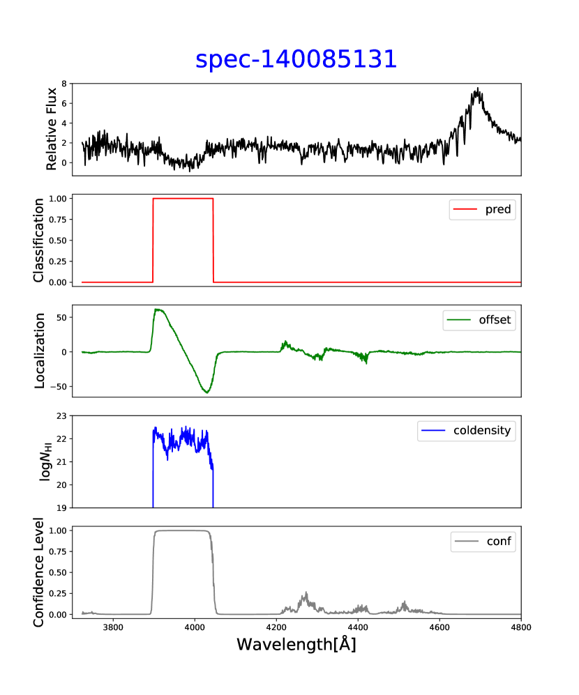
Figure 7: Four outputs for every window: ’pred’, ’offset’, ’coldensity’ and ’conf’ . The red line is ’pred’, the value for 120 pixels near the center of a DLA is 1 and for other pixels is 0. The green line is ’offset’, it shows the distance between every pixel and the center pixel of a DLA. The value of offset is close to 0 for the pixles without a DLA. The blue line is the column density. The last grey line is the confidence level. This is an example with high confidence level, the confidence value for pixels with a DLA is above 0.9.

3.3 Hyperparameter Search

There are 26 parameters for this CNN model which determines the size of each layer. We have conducted the hyperparameter search for these parameters. Since we optimize the hyperparameters for the DESI mock spectra, our best combination of the hyperparameters is different from that of Parks et al. (2018) which is optimized for SDSS spectra.

A normal important parameter in this algorithm is the input size of the spectral window. In Parks et al. (2018), each QSO spectrum was cut into windows with the size of 400 pixels, and the classification accuracy depends on the size of the window. We have measured the classification accuracy by changing the window size from 300 pixels to 700 pixels, with the step of 100 pixels. We find that a window size of 600 pixels, combined with the hyperparameters determined above, giving the best accuracy.

4 Validation

4.1 Purity and completeness

Beside the classification accuracy, the purity and completeness are also important results for the CNN model. Purity and completeness are both for DLAs because TN samples are excluded. The confusion matrix defination is similar to Table 6 but without TN samples. GroundTruth stands for the label of DLAs in mock spectra and the prediction is the DLA label from our CNN. A DLA in mock spectra will have the GroundTruth value as 1. Similarly, the prediction of 1 means a DLA is detected by the CNN model. If our CNN missed one DLA, then a FN sample is produced (GroundTruth as 1 but prediction as 0). After the prediction, two DLA catalogs are generated. One is produced by the CNN model and another one is the mock DLA catalog. For each DLA in the mock catalog, we search DLAs in the same sightline among the predicted DLA catalog and then compare the distance between the center of these two DLAs. If the distance is less than 10 $\rm{\AA}$, this is a true positive prediction and these two DLAs will be both marked as TP. We choose 10 $\rm{\AA}$ as the critical value to make the redshift estimate for TP DLAs has less than 0.008. This difference in redshift estimate is acceptable. This critical value can make the CNN model provide accurate redshift estimate ($<0.008$) and high classification accuracy ($>97\%$) when comparing the result to mock spectra. If the distance is above 10 $\rm{\AA}$, this is a false negative prediction and the DLA in mock catalog will be marked as FN. After that, DLAs in predicted catalog without a TP label will be considered as a FP sample. The purity and completeness are defined as

$$Purity=\frac{TP}{TP+FP}$$ (4)

$$Completeness=\frac{TP}{TP+FN}$$ (5)

By changing the critical value of $C_{\rm min}$, we obtain different DLA catalogs. The default critical value is 0.5 as introduced in Section 3.2. Changing this critical value changes the FP rate and FN rate, and yields different DLA catalogs. The higher critical values improve the purity but reduce the completeness. To balance the purity and completeness, this value is still set as 0.5 in our model.

We have calculated the purity and completeness for different S/N and column densities. The results are shown in Figure 8 and Figure 9. For DLAs in spectra with S/N $>3$, our model can achieve both purity and completeness more than 90$\%$ for almost all column density levels. Although efforts have been made to optimize the DLA identification accuracy, FN and FP cases are inevitable. The majority of these occur in spectra with low S/N ($<3$). As shown in Figure 10, these are examples which are difficult to classify even for an expert.

We also test our model on desiY1-0.14 mock spectra. This mock spectra contains both DLAs and BALs. We show the purity and completeness in Figure 20. The completeness is still as good as shown in Figure 9. The purity drops about 10$\%$ to 20$\%$ in different bins. This is because some BALs are identified as DLAs. Nevertheless, the DESI has a formal BAL catalog which will get rid of more than $98.6\%$ BALs Guo & Martini (2019) from the catalog. Then, we can run DLA finder on the BAL-removed spectra. Therefore, we think that the purity result shown in Figure 8 is still valid.

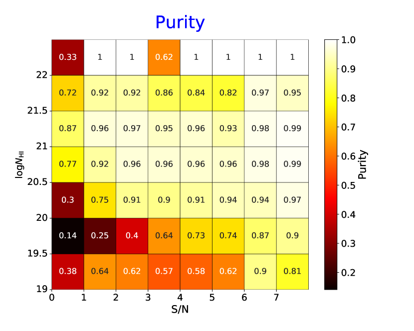
Figure 8: Purity results for different S/N levels and column densities using desi-Y1 mock spectra. This is the result choosing the critical value of $C_{\rm min}$ as 0.5. Some bins on the top has the value 1, this is because there are few DLAs with $\log{N_{\rm{HI}}}$ above 22 from Y1 mock. For example, there are just 2 DLAs in the bin with S/N 4 to 5 and $\log{N_{\rm{HI}}}$ above 22. The DLA finder detects them both and no FP samples, so the purity goes to 1. There are just 5 DLAs in the bin with S/N 3 to 4 and $\log{N_{\rm{HI}}}$ above 22. The DLA finder detects three of them and produce 2 FP samples, so the purity goes down to 0.6. That is why the purity for high column density DLAs changes a lot in different bins.

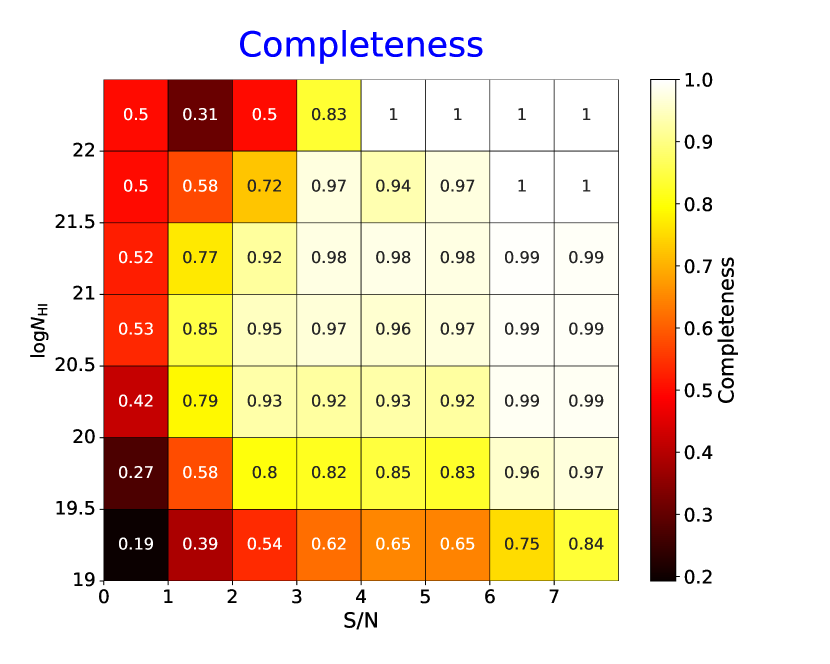
Figure 9: Completeness results for different S/N levels and column densities using desi-Y1 mock spectra. This is the result choosing the critical value of $C_{\rm min}$ as 0.5. Some bins on the top has the value 1, this is because there are few DLAs with $\log{N_{\rm{HI}}}$ above 22 from Y1 mock. For example, there are just 2 DLAs in the bin with S/N 4 to 5 and $\log{N_{\rm{HI}}}$ above 22. The DLA finder detects them both, so the purity goes to 1. There are just 5 DLAs in the bin with S/N 3 to 4 and $\log{N_{\rm{HI}}}$ above 22. The DLA finder detects four of them and misses one DLA, so the purity goes down to 0.8. That is why the completeness for high column density DLAs changes a lot in different bins.

Figure 10: validation samples: red lines are DLAs detected by our CNN model and blues lines are the DLAs in mock spectra. (a)(b) TP case, our model can detect DLAs with different column density levels. Even sub-DLAs can be characterized. (c) FP case, the DLA finder identifies a DLA in this window but there is no such a DLA in the mock catalog. Lower panel of (c) is the same spectra as upper panel but with a higher S/N. It is clear there is no DLA if we check the high S/N spectra. But this is very difficult to identify even for the human being in upper panel of figure (c) because of the low S/N. (d) FN sample, the DLA finder misses a sub-DLA in this wavelength range. Lower panel of (d) is the same spectra as upper panel but with higher S/N. This shows a missing sub-DLA with low S/N($<$2). The flux range for lower panel and upper panel of (c)(d) is quite different because a random array as the noise is inserted to get a lower S/N

4.2 Redshift Estimation

According to the offset label predicted by CNN model, we locate the central wavelength of DLAs. This can be used to estimate the redshift of DLAs. The direct result for our model is the DLA location in every window. We need to transfer this result to the location in the sightline. This procedure is similar in Parks et al. (2018). We make the histogram of all the offset values, and a cluster of values at the center of a true DLA is expected. A confidence parameter for the whole spectra is further defined as the sum of the histogram over the nearest five pixels. After normalizing by the 9-pixel median filter, the maximum limit is set to one. Every detection with this confidence parameter above the critical value are considered as a DLA. Then we can calculate the redshift of DLAs according to the central wavelength.

The difference of the redshift estimation compared to the true value (value in mock spectra) is shown in Figure 11. This result is for the spectra in ’desi-0.2-100’ mock spectra. The mean value of the difference is -0.00012, and the standard deviation $\sigma(z)$ is 0.002.

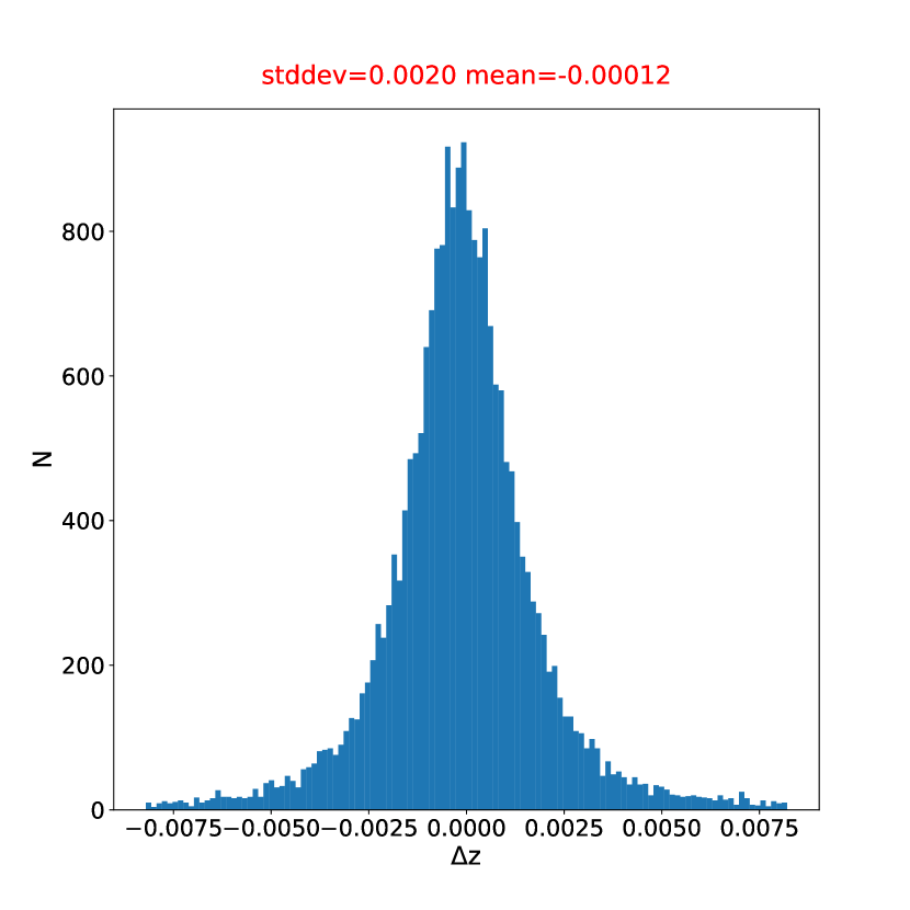
Figure 11: Redshift estimation for the DLAs matched between the CNN model and the true value in mock spectra with $S/N>3$ and $log(N_{\rm{HI}})>20.0$.

4.3 Column Density Estimation

Our model can also give the estimation for the column density of DLAs. For every window of spectra, we can get an estimated value of the column density. After locating the central wavelength of a DLA, we can get the $N_{\rm{HI}}$ estimation results for the 40 pixels near the center, and take the average value of these 40 $N_{\rm{HI}}$ estimate as the final estimate. The difference of the column density estimation compared to the true value is shown in Figure 12. This result is for the spectra in ’desi-0.2-100’ mock spectra. The mean value of the difference is -0.007, and the standard deviation $\sigma(\log{N_{\rm{HI}}})$ is 0.17.

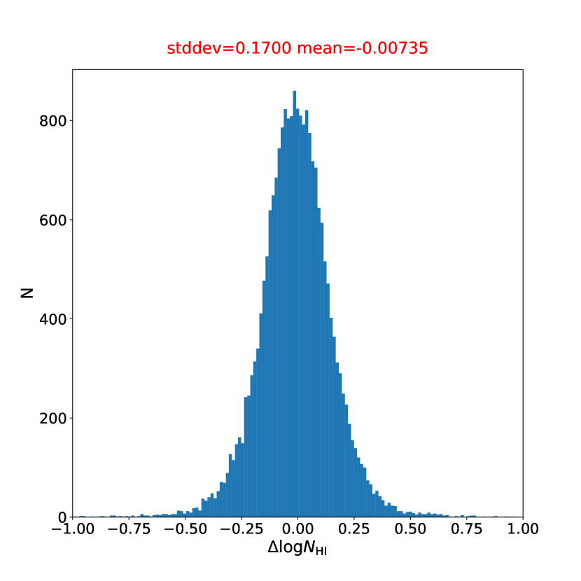
Figure 12: The column density estimation for the DLAs matched between the CNN model and the true value in mock spectra with $S/N>3$ and $log(N_{\rm{HI}})>20.0$ .

5 Comparison with Gaussian Process Model

Recent advances in Gaussian Process (GP) model facilitated the investigation of detecting DLAs from SDSS(Garnett et al., 2017; Ho et al., 2020, 2021). Ho et al. (2021) presented a DLA catalog from SDSS DR16Q, with an improved GP model. Currently, it might be the most solid approach to compare the performance between CNN model and GP model using DESI mock spectra with a given DLA catalog.

Here we briefly introduce their GP model based on the Bayesian model selection in Ho et al. (2020). A set of models ${\mathcal{M}_{i}}$ are developed, including the model without DLAs ($\mathcal{M}_{\rm{\neg DLA}}$), the models with 4 DLAs (${\mathcal{M}_{\rm{DLA(i)}}}_{i=1}^{4}$), and the model with sub-DLAs ($\mathcal{M}_{\rm{sub}}$). These models use Gaussian Processes to describe the QSO emission function, a qso’s true emission spectrum $f(\lambda)$. Then they add the instrumental noise and absorption due to the intervening intergalactic medium (IGM) to obtain the observed flux as a function $y(\lambda)$. With a given spectroscopic sightline $\mathcal{D}$, they can evaluate the posterior probability of these model based on Bayes’s rule:

$$Pr(\mathcal{M}\mid\mathcal{D})=\frac{p(\mathcal{D}\mid\mathcal{M})Pr(\mathcal{M})}{\sum_{i}p(\mathcal{D}\mid\mathcal{M}_{i})Pr(\mathcal{M}_{i})}$$ (6)

where $p(\mathcal{D}\mid\mathcal{M})$ is the model evidence of the QSO spectrum $\mathcal{D}$ given model $\mathcal{M}$, $Pr(\mathcal{M})$ is the prior probability of model $\mathcal{M}$, and the denominator on the right-hand-side is the sum of posterior probabilities of all models in consideration.

Following the pipeline described in Ho et al. (2020), we firstly retrained the null model $M_{\rm{\neg DLA}}$ using 70255 spectra without DLAs in the ’desiY1-0.2-DLA’ mock. Then we extend the null model $M_{\rm{\neg DLA}}$ to a model with k intervening DLAs, $\mathcal{M}_{\rm{DLA(k)}}$(k up to 4). The model prior and model evidence for these models are approximated by using the ’desiY1-0.2-DLA’ mock DLA catalog. Applying the new GP model, we obtain a DLA catalog of 248512 sightlines in the ’desiY1-0.2-DLA’ mock. Note that the default Voigt profile they use in Ho et al. (2020) includes Ly$\alpha$, Ly$\beta$, and Ly$\gamma$ absorption, but we set the number of absorption lines $num\_lines$ to one since this mock only contains Ly$\alpha$ absorption lines. Also we modify the parameters about the mininum distance between DLAs $min\_z\_separation$ to zero since we want to identify very close overlapping DLAs. All codes related to GP are available at https://github.com/zoujiaqi99/GP_DLA_DESI.

With $S/N>3$ and $log(N_{\rm{HI}})>20.0$, there are 18613 real DLAs in the mock DLA catalog. 17571 DLAs are predicted by the CNN model while 23212 DLAs are predicted by the GP model. As discussed in Section 4, we also present the purity and completeness for S/N and column densities level as shown in Figure 16 and Figure 17. For GP model, completeness and purity are both greater than 88$\%$ for $S/N>3$. Note that our CNN model can measure the redshift and column density with $log(N_{\rm{HI}})>19.3$. The GP model we used provides model posterior probability of whether the sightline containing absorbers with log(NHI) $<$ 20.0, but does not save the exact redshifts or column densities. This is due to the difference in training sets between the CNN and GP methods. We fairly compare the two models under the same conditions in this manuscript. However, the DESI mock spectra allow us to build datasets with low $N_{\rm{HI}}$ absorbers to re-train the GP model in order to decrease its minimum to $log(N_{rm{HI}})=19.3$.

Figure 13 and 14 show histograms of the offsets in redshift and $N_{\rm{HI}}$ between the GP model’s predictions and real values in the mock catalog. The mean redshift offset is 0.00001 with a standard deviation of 0.0016. The mean log column density offset is $\Delta log(N_{\rm{HI}})=0.005$ with standard deviation of 0.13 dex.

We also present the column density distribution function (CDDF) in Figure 15. This figure contains both CNN DLA catalog and GP DLA catalog in comparison to the real mock DLA catalog with $z<3.8$. The distribution of both models does not significantly differ from that of the real catalog. Due to the more accurate $N_{\rm{HI}}$ estimation, the GP model is in a better agreement with the real catalogue except for the Monte Carlo sampling boundary($log(N_{\rm{HI}})=20.0$), where induces the over-detection of absorbers with $log(N_{\rm{HI}})<20.0$. Ho et al. (2020) showed the CDDF and concluded that the previous CNN model (Parks et al., 2018) is failing to detect $>60\%$ of DLAs with $log(N_{\rm{HI}})>21$. This problem does not exist in our results. The lack of high column density absorbers in the Parks catalogue may be due to a lack of high column density systems in their training set.

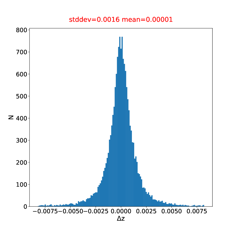
Figure 13: The redshift estimation for the DLAs matched between the Gaussian Process model and the true value in mock spectra with $S/N>3$ and $\log{N_{\rm{HI}}}>20.0$

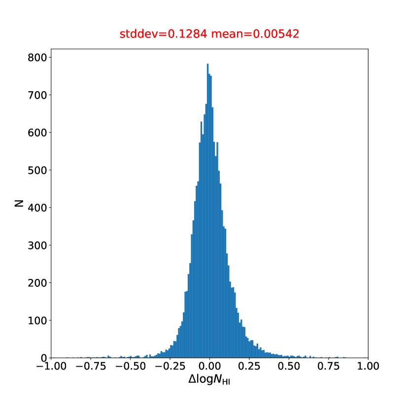
Figure 14: The column density estimation for the DLAs matched between the Gaussian Process model and the true value in mock spectra with $S/N>3$ and $\log{N_{\rm{HI}}}>20.0$

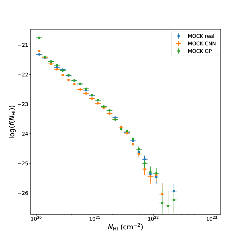
Figure 15: The CDDF from both CNN DLA catalog and GP DLA catalog in comparison to the real mock DLA catalog with $z<3.8$. The error bars in y-axis represent the 68$\%$ confidence limits.

Compare the performance of the same mock, we find that the CNN model performs better in purity and completeness while the GP model has a more accurate estimation of column density. In terms of BAO measurement using DESI Y1 mock, the CNN model is more effective as described in Section 6. Besides, GP model takes 8 to 10 times longer than CNN model to predict the same dataset. Consequently, a combined DLA catalog that takes the best of both models might be a better choice for DESI real data. CNN can be mainly used to detect DLAs and estimate redshift because of the higher completeness and purity. GP can be applied to further improve the column density estimate. The DLAs detected by GP are an important part to complete the DLA catalog. Besides, we can also provide a DLA catalog which only contains DLAs detected by both CNN and GP. The DLAs detected by both algorithms maybe a smaller sample but with high confidence.

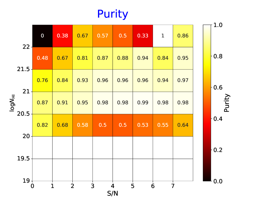
Figure 16: GP purity results for different S/N levels and column densities using desi-Y1 mock spectra. Here we only select absorbers with $N_{\rm{HI}}>20.0$ to provide a simple comparison. Because the current GP model is well developed only using $N_{\rm{HI}}>20.0$ absorbers.

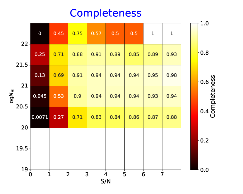
Figure 17: GP completeness results for different S/N levels and column densities using desi-Y1 mock spectra. Here we only select absorbers with $N_{\rm{HI}}>20.0$ to provide a simple comparison. Because the current GP model is well developed only using $N_{\rm{HI}}>20.0$ absorbers.

6 BAO fitting analysis

6.1 BAO fitting procedure

After the DLA catalogs are generated, we tested the influence of different DLA catalogs on the measurement of BAO fitting. Two different DLAs catalogs are generated. One catalog contains all the DLAs in the mock spectra, we will take this catalog as the real DLA catalog. Another catalog only contains the DLAs detected by our CNN model. The BAO fitting is conducted using the Ly$\alpha$-QSO cross correlation and Ly$\alpha$-Ly$\alpha$ auto correlation. According to the definition of du Mas des Bourboux et al. (2020), the flux-transmission field is

$$\delta_{q}(\lambda)=\frac{f_{q}(\lambda)}{F(\lambda)C_{q}(\lambda)}-1$$ (7)

Where $f_{q}(\lambda)$ is the observed flux, $F(\lambda)C_{q}(\lambda)$ is the mean expected flux. The BAO fitting procedure is followed by the pipeline in du Mas des Bourboux et al. (2020). For the Ly$\alpha$-QSO cross correlation and Ly$\alpha$-Ly$\alpha$ auto correlation, the first step is to do the continuum fitting. In this step, we obtain the flux-transmission field from the observed flux and the mean expected flux. DLAs should be masked in this step.

The next steps and the meaning of parameters are described in details in du Mas des Bourboux et al. (2020). The pipeline we use for these steps is called ’PICCA’ (https://github.com/igmhub/picca), which was developed by the eBOSS Ly$\alpha$ working group (du Mas des Bourboux et al., 2020). This pipeline can mask DLAs for the BAO fitting if we provide a DLA catalog as an input.

In this fitting, we have set the following parameters in PICCA as free parameter to fit. The high column density systems(HCD) are also considered in the fitting:

1. $\alpha_{\parallel}$, $\alpha_{\perp}$: BAO-peak position parameters.

2. $b_{Ly\alpha}$, $\beta_{Ly\alpha}$: bias parameters for $Ly\alpha$ absorption.

3. $b_{HCD}$, $\beta_{HCD}$: bias parameters for HCD systems.

Other parameters in PICCA has been set as fixed parameter.

6.2 BAO fitting results

We have used the ’desiY1-0.2-DLA’ mock spectra to do the BAO fitting analysis. This mock spectra contains DLAs and HCDs but do not have metal components.

This mock spectra contains 212238 sightlines with 36212 DLAs and 43909 sub-DLAs. Our CNN model has detected 43530 DLA candidates and 19687 sub-DLAs. 38410 DLA candidates are detected by GP. The sub-DLAs in mock catalog are added to GP catalog when we do the BAO fitting. FP and FN samples are inevitable from the lower S/N spectra ($<3$). We have conducted the Ly$\alpha$-QSO cross correlation and Ly$\alpha$-Ly$\alpha$ auto correlation by masking these two different DLA catalogs. We also plot the fitting result if we do not mask any DLAs and mask the DLA catalog generated by Gaussian Process (GP) which were described in Section 5. The results are shown in Figure 18.

Figure 18: BAO fitting result:(a)the QSO-Lya cross-correlation (b) Lya-Lya auto-correlation. The red line is the best-fit model by masking the DLAs in the mock catalog. The black dashed line is the best-fit model by masking DLAs detected by our CNN model. The blue dashed line is the best-fit model if we do not mask any DLA. The yellow dashed line is the best-fit model by masking DLAs detected by Gaussian Process. The grey points are the data points from the analyse by masking the DLAs in mock spectra.

After masking DLAs, the reduced $\chi^{2}$ of the fitting decreases from 1.136 to 1.081. Impact of DLAs on BAO fitting is obvious in the auto-correlation fitting. The BAO fitting result from the mock DLAs catalog was set as the ground-truth. Two parameters describing the position of BAO peak Busca et al. (2013), $\alpha_{\parallel}$ and $\alpha_{\perp}$ are estimated to quantify the fitting results. The best fitting parameters are shown in Table 7. This table also contains the standard deviation for $\alpha_{\parallel}$, $\alpha_{\perp}$ and the reduced $\chi^{2}$ in two different fittings. The difference of the results can be quantified by the following equations:

Table 7: Best fitting parameters

parameters	DLA mock	DLA CNN	DLA GP	No Mask
$\alpha_{\parallel}$	0.981	0.983	0.977	0.992
$\sigma$	0.0173	0.0174	0.0195	0.0212
$d_{\alpha_{\parallel}}$		0.16$\%$	0.41$\%$	1.12$\%$
ratio		0.116	0.209	0.636
$\alpha_{\perp}$	1.019	1.025	1.025	1.028
$\sigma$	0.0172	0.0177	0.0194	0.0227
difference		0.61$\%$	0.61$\%$	0.94$\%$
ratio		0.349	0.304	0.523
$\chi^{2}/DOF$	1.081	1.091	1.098	1.136

$$d_{\alpha_{\parallel}}=\frac{|\alpha_{\parallel}(mock)-\alpha_{\parallel}(pred)|}{\alpha_{\parallel}(mock)}$$ (8)

$$d_{\alpha_{\perp}}=\frac{|\alpha_{\perp}(mock)-\alpha_{\perp}(pred)|}{\alpha_{\perp}(mock)}$$ (9)

Where $a_{\parallel}(mock)$ is the fitting results of $\alpha_{\parallel}$ parameter by using the mock DLA catalog, and $a_{\parallel}(pred)$ stands for the results using our DLA catalog. Similarly, $a_{\perp}(mock)$ and $a_{\perp}(pred)$ are fitting value of $\alpha_{\perp}$ parameter using mock DLA catalog and our DLA catalog. We also define the ratio of difference and error as below:

$${ratio}_{\alpha_{\parallel}}=\frac{|\alpha_{\parallel}(mock)-\alpha_{\parallel}(pred)|}{\sigma\alpha_{\parallel}(mock)}$$ (10)

$${ratio}_{\alpha_{\perp}}=\frac{|\alpha_{\perp}(mock)-\alpha_{\perp}(pred)|}{\sigma\alpha_{\perp}(mock)}$$ (11)

The differences between these two fitting results are less than $0.61\%$. This difference is lower than the statistical error using the DESI first year mock spectra (above $1.7\%$ shown in Table 7). The statistical error will be reduced in the next 4 years DESI survey. With increasing S/N in the next few years, the DLA finder can give a better detection than the first year. And this difference can be further reduced. The DLA catalog generated by our CNN model can be used for the BAO fitting analysis.

We also compare the performance on correlation fitting using DLA catalog generated by GP. The difference of best fitting parameters between GP and mock shown in Table 7 are about 0.25$\%$ larger than the difference between CNN and mock. But this difference is still less than the statistical error. So the BAO fitting result for the mock spectra is not affected much in any of the analyses presented. CNN DLA catalog can give a better BAO analysis support because of the higher completeness. The difference of fitting is clear when checking the difference of best fitting parameters value. We have also plotted the result in Figure 19. Details about more parameters are shown in 8. This BAO analysis result is based on the mock spectra for DESI first year’s survey. We plan to use different mock spectra to do the fitting comparison in the future.

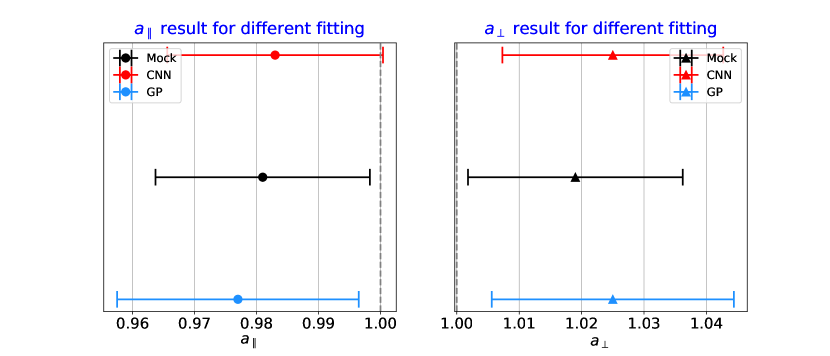
Figure 19: The value and error bar for three different fittings: masking DLAs in the mock catalog, masking DLAs detected by CNN and masking DLAs detected by GP. It is clear that the result from masking GP DLA catalog has larger difference between the mock DLA catalog. The grey line is the theoretical value for these two parameters.

7 Conclusion

In this manuscript, we have applied the deep learning techniques on QSO spectra to classify and characterize the damped Ly$\alpha$ systems (DLAs). We improved the CNN model created by Parks et al. (2018) using DESI mock spectra to make it work successfully on DESI spectra. We optimize the preprocess, training procedure, parameter selection and the performance on low S/N and high column density DLAs. Our model can give effective and accurate estimation about redshift and column density. We also improve the performance for CNN on low S/N spectra by smoothing the input flux,this method may also be used to other algorithm for low S/N signals. This CNN model can detect DLAs even when the S/N of DLAs is only about 1. We believe that there is still room to further improve this algorithm.

Besides, our DLA catalog can also help to do the BAO analysis. When we want to use correlation to do the BAO fitting, a DLA catalog is necessary. The results produced by our DLA catalog are very close to the real mock results, within the difference about $0.61\%$ for the best fitting parameters.

Finally, we compare our CNN DLA Finder with the Gaussian Process model from Ho et al. (2020) based on DESI mock spectra. Note that it may not be possible to show all the advantages and disadvantages of the two models due to the limitation of the mock. However, It is sufficient to see the differences between the two models by comparing their predictions with the mock truths. CNN model has a higher completeness and purity on detecting DLAs. The fitting differences using CNN and GP DLA catalog are less than the statistical error on BAO fitting using Y1 mock spectra. The CNN results yield a systematic uncertainty $0.25\%$ less than that of GP. The BAO fitting result is not affected much by using either DLA finders. Both algorithms can estimate the redshift of DLAs well. While the Gaussian Process model has more accurate column density estimation. Combining the catalogs given by the two models, we can obtain a credible DLA catalog that can be widely used for real DESI spectra release.

8 Ackowledgement

This research is supported by the Director, Office of Science, Office of High Energy Physics of the U.S. Department of Energy under Contract No. DE–AC02–05CH11231, and by the National Energy Research Scientific Computing Center, a DOE Office of Science User Facility under the same contract; additional support for DESI is provided by the U.S. National Science Foundation, Division of Astronomical Sciences under Contract No. AST-0950945 to the NSF’s National Optical-Infrared Astronomy Research Laboratory; the Science and Technologies Facilities Council of the United Kingdom; the Gordon and Betty Moore Foundation; the Heising-Simons Foundation; the French Alternative Energies and Atomic Energy Commission (CEA); the National Council of Science and Technology of Mexico; the Ministry of Economy of Spain, and by the DESI Member Institutions. The authors are honored to be permitted to conduct scientific research on Iolkam Du’ag (Kitt Peak), a mountain with particular significance to the Tohono O’odham Nation. BW, JZ, ZC supported by the National Key R$\&$D Program of China (grant No.2018YFA0404503), the National Science Foundation of China (grant No. 12073014). AFR acknowledges support FSE funds trough the program Ramon y Cajal (RYC-2018-025210) of the Spanish Ministry of Science and Innovation. VI is supported by the Kavli foundation. BW, JZ, ZC acknowledge the fruitful discussion with Dr. Tao Qin at Microsoft Research Asia. BW and JZ appreciate the great help from Huaizhe Xu in International Digital Economy Academy(IDEA). The authors also appreciate Mr. Ming-Feng Ho from University of California Riverside for the great help about running Gaussian Process algorithm.

Appendix A BAO combine fitting aprameters

Table 8: Best fitting parameters

parameters	DLA mock	DLA CNN	DLA GP	No Mask
$\alpha_{\parallel}$	0.981	0.983	0.977	0.992
$\sigma$	0.0173	0.0174	0.0195	0.0212
$\alpha_{\perp}$	1.019	1.025	1.025	1.028
$\sigma$	0.0172	0.0177	0.0194	0.0227
$beta_{LYA}$	1.5603	1.5515	1.6684	1.4066
$\sigma$	0.0259	0.0265	0.0584	0.0214
$bias_{LYA}$	-0.1359	-0.1391	-0.0755	-0.1581
$\sigma$	0.0013	0.0014	0.0018	0.0015
$bias_{eta}(LYA)$	-0.2186	-0.2224	-0.2077	-0.2292
$\sigma$	0.0021	0.0022	0.0028	0.0021
$beta_{HCD}$	0.8237	0.8703	0.8710	0.8891
$\sigma$	0.0689	0.0685	0.0850	0.0657
$bias_{HCD}$	-0.0591	-0.0621	-0.0701	-0.0795
$\sigma$	0.0022	0.0022	0.0022	0.0028
$\chi^{2}/DOF$	1.081	1.091	1.098	1.136

Appendix B Purity and Completeness for desiY1-0.14 mock spectra

Figure 20: We have applied our CNN model on desiY1-0.14 mock spectra. This mock spectra contains both DLAs and BALs. The purity and completeness are shown in (a) and (b). The minimum S/N for this mock is 1.0, and thus the left panel (S/N $<0$) is blank. The completeness is still above 96$\%$ for S/N$>$3 spectra. The purity drops about 10$\%$ to 20$\%$ in different bins. Nevertheless, the DESI has a formal BAL catalog which will get rid of more than $98.6\%$ BALs from the catalog. Then, we can run DLA finder on the BAL-removed spectra. Therefore, we think that the purity result shown in Figure8 is still valid.

Appendix C DLA detection in SDSS spectra

In Ho et al. (2021), the author mentioned that the previous version of CNN DLA finderParks et al. (2018) missed high column density DLAs in two SDSS spectra. We test our model on these two spectra, both the DLAs and subDLAs can be detected as shown in Figure 21

Figure 21: We have applied our CNN model on these two spectra mentioned by Ho et al. (2021). It is clear that the DLA and subDLA candidates are detected.

References

- Bird et al. (2014) Bird, S., Vogelsberger, M., Haehnelt, M., et al. 2014, MNRAS, 445, 2313, doi: 10.1093/mnras/stu1923
- Busca et al. (2013) Busca, N. G., Delubac, T., Rich, J., et al. 2013, A&A, 552, A96, doi: 10.1051/0004-6361/201220724
- Cai et al. (2016) Cai, Z., Fan, X., Peirani, S., et al. 2016, ApJ, 833, 135, doi: 10.3847/1538-4357/833/2/135
- Cai et al. (2017) Cai, Z., Fan, X., Bian, F., et al. 2017, ApJ, 839, 131, doi: 10.3847/1538-4357/aa6a1a
- Chabanier et al. (2021) Chabanier, S., Etourneau, T., Le Goff, J.-M., et al. 2021, arXiv e-prints, arXiv:2107.09612. https://arxiv.org/abs/2107.09612
- DESI Collaboration et al. (2016a) DESI Collaboration, Aghamousa, A., Aguilar, J., et al. 2016a, arXiv e-prints, arXiv:1611.00036. https://arxiv.org/abs/1611.00036
- DESI Collaboration et al. (2016b) —. 2016b, arXiv e-prints, arXiv:1611.00037. https://arxiv.org/abs/1611.00037
- Dey et al. (2019) Dey, A., Schlegel, D. J., Lang, D., et al. 2019, AJ, 157, 168, doi: 10.3847/1538-3881/ab089d
- Draine (2011) Draine, B. T. 2011, Physics of the Interstellar and Intergalactic Medium
- du Mas des Bourboux et al. (2020) du Mas des Bourboux, H., Rich, J., Font-Ribera, A., et al. 2020, ApJ, 901, 153, doi: 10.3847/1538-4357/abb085
- Farr et al. (2020) Farr, J., Font-Ribera, A., du Mas des Bourboux, H., et al. 2020, J. Cosmology Astropart. Phys, 2020, 068, doi: 10.1088/1475-7516/2020/03/068
- Finley et al. (2013) Finley, H., Petitjean, P., Pâris, I., et al. 2013, A&A, 558, A111, doi: 10.1051/0004-6361/201321745
- Font-Ribera & Miralda-Escudé (2012) Font-Ribera, A., & Miralda-Escudé, J. 2012, J. Cosmology Astropart. Phys, 2012, 028, doi: 10.1088/1475-7516/2012/07/028
- Fumagalli et al. (2011) Fumagalli, M., Prochaska, J. X., Kasen, D., et al. 2011, MNRAS, 418, 1796, doi: 10.1111/j.1365-2966.2011.19599.x
- Gardner et al. (1997) Gardner, J. P., Sharples, R. M., Frenk, C. S., & Carrasco, B. E. 1997, ApJ, 480, L99, doi: 10.1086/310630
- Garnett et al. (2017) Garnett, R., Ho, S., Bird, S., & Schneider, J. 2017, MNRAS, 472, 1850, doi: 10.1093/mnras/stx1958
- Gonzalez-Morales & DESI Lyman Working Group (In preparation) Gonzalez-Morales, A. X., & DESI Lyman Working Group. In preparation
- Grudić et al. (2020) Grudić, M. Y., Guszejnov, D., Hopkins, P. F., Offner, S. S. R., & Faucher-Giguère, C.-A. 2020, arXiv e-prints, arXiv:2010.11254. https://arxiv.org/abs/2010.11254
- Guo & Martini (2019) Guo, Z., & Martini, P. 2019, ApJ, 879, 72, doi: 10.3847/1538-4357/ab2590
- Herrera-Alcantar (2020) Herrera-Alcantar, H. K. 2020, Master’s thesis, Universidad de Guanajuato
- Ho et al. (2020) Ho, M.-F., Bird, S., & Garnett, R. 2020, MNRAS, 496, 5436, doi: 10.1093/mnras/staa1806
- Ho et al. (2021) —. 2021, arXiv e-prints, arXiv:2103.10964. https://arxiv.org/abs/2103.10964
- Jolly et al. (2020) Jolly, J.-B., Knudsen, K. K., & Stanley, F. 2020, MNRAS, 499, 3992, doi: 10.1093/mnras/staa2908
- Krogager et al. (2020) Krogager, J.-K., Møller, P., Christensen, L. B., et al. 2020, MNRAS, 495, 3014, doi: 10.1093/mnras/staa1414
- Lee et al. (2020) Lee, C. C., Webb, J. K., & Carswell, R. F. 2020, MNRAS, 491, 5555, doi: 10.1093/mnras/stz3170
- Lee et al. (2014) Lee, K.-G., Hennawi, J. F., Stark, C., et al. 2014, ApJ, 795, L12, doi: 10.1088/2041-8205/795/1/L12
- Li et al. (2021) Li, Z., Horowitz, B., & Cai, Z. 2021, ApJ, 916, 20, doi: 10.3847/1538-4357/ac044a
- Liske et al. (1998) Liske, J., Webb, J. K., & Carswell, R. F. 1998, MNRAS, 301, 787, doi: 10.1046/j.1365-8711.1998.02048.x
- McDonald (2003) McDonald, P. 2003, ApJ, 585, 34, doi: 10.1086/345945
- McGreer et al. (2013) McGreer, I. D., Jiang, L., Fan, X., et al. 2013, ApJ, 768, 105, doi: 10.1088/0004-637X/768/2/105
- McQuinn (2016) McQuinn, M. 2016, ARA&A, 54, 313, doi: 10.1146/annurev-astro-082214-122355
- Noterdaeme et al. (2019) Noterdaeme, P., Balashev, S., Krogager, J. K., et al. 2019, A&A, 627, A32, doi: 10.1051/0004-6361/201935371
- Noterdaeme et al. (2009) Noterdaeme, P., Petitjean, P., Ledoux, C., & Srianand, R. 2009, A&A, 505, 1087, doi: 10.1051/0004-6361/200912768
- Noterdaeme et al. (2012a) Noterdaeme, P., Petitjean, P., Carithers, W. C., et al. 2012a, A&A, 547, L1, doi: 10.1051/0004-6361/201220259
- Noterdaeme et al. (2012b) Noterdaeme, P., Laursen, P., Petitjean, P., et al. 2012b, A&A, 540, A63, doi: 10.1051/0004-6361/201118691
- Parks et al. (2018) Parks, D., Prochaska, J. X., Dong, S., & Cai, Z. 2018, MNRAS, 476, 1151, doi: 10.1093/mnras/sty196
- Pérez-Ràfols et al. (2018) Pérez-Ràfols, I., Font-Ribera, A., Miralda-Escudé, J., et al. 2018, MNRAS, 473, 3019, doi: 10.1093/mnras/stx2525
- Péroux et al. (2003) Péroux, C., McMahon, R. G., Storrie-Lombardi, L. J., & Irwin, M. J. 2003, MNRAS, 346, 1103, doi: 10.1111/j.1365-2966.2003.07129.x
- Prochaska & Herbert-Fort (2004) Prochaska, J. X., & Herbert-Fort, S. 2004, PASP, 116, 622, doi: 10.1086/421985
- Prochaska et al. (2005) Prochaska, J. X., Herbert-Fort, S., & Wolfe, A. M. 2005, ApJ, 635, 123, doi: 10.1086/497287
- Prochaska et al. (2015) Prochaska, J. X., O’Meara, J. M., Fumagalli, M., Bernstein, R. A., & Burles, S. M. 2015, ApJS, 221, 2, doi: 10.1088/0067-0049/221/1/2
- Prochaska & Wolfe (1997) Prochaska, J. X., & Wolfe, A. M. 1997, ApJ, 487, 73, doi: 10.1086/304591
- Rahmati et al. (2014) Rahmati, A., Cravens, T., Larson, D. E., et al. 2014, in AGU Fall Meeting Abstracts, Vol. 2014, P51B–3932
- Rauch (1998) Rauch, M. 1998, ARA&A, 36, 267, doi: 10.1146/annurev.astro.36.1.267
- Wolfe et al. (2005) Wolfe, A. M., Gawiser, E., & Prochaska, J. X. 2005, ARA&A, 43, 861, doi: 10.1146/annurev.astro.42.053102.133950
- Wolfe et al. (1986) Wolfe, A. M., Turnshek, D. A., Smith, H. E., & Cohen, R. D. 1986, ApJS, 61, 249, doi: 10.1086/191114
- Yèche et al. (2020) Yèche, C., Palanque-Delabrouille, N., Claveau, C.-A., et al. 2020, Research Notes of the American Astronomical Society, 4, 179, doi: 10.3847/2515-5172/abc01a
- Zafar et al. (2013) Zafar, T., Péroux, C., Popping, A., et al. 2013, A&A, 556, A141, doi: 10.1051/0004-6361/201321154