Observability, Dominance, and Induction in Learning Models

Abstract

Learning models do not in general imply that weakly dominated strategies are irrelevant or justify the related concept of “forward induction,” because rational agents may use dominated strategies as experiments to learn how opponents play, and may not have enough data to rule out a strategy that opponents never use. Learning models also do not support the idea that the selected equilibria should only depend on a game’s normal form, even though two games with the same normal form present players with the same decision problems given fixed beliefs about how others play. However, playing the extensive form of a game is equivalent to playing the normal form augmented with the appropriate terminal node partitions so that two games are information equivalent, i.e., the players receive the same feedback about others’ strategies.

Keywords: learning in games, equilibrium refinements, iterated dominance, forward induction

Introduction

The learning in games literature asks which equilibria are likely to persist in environments where new players are initially uncertain about the prevailing strategies and learn about the strategy distribution by repeatedly playing the game. One reason for the success of strategic stability and associated refinements is that they select intuitive equilibria in signaling games, as shown by [1] and [5]. Learning models make similar predictions in these games ([16], [12], [6]). In this paper, we show that these two sorts of refinements can have very different predictions in other games. Specifically, we show that learning models do not in general support either the iterated deletion of weakly dominated strategies or the related concept of “forward induction.” We also show that learning models support only some of the invariance axioms proposed by [23] and [9].

There are two distinct reasons that the outcomes of learning models need not satisfy forward induction or iterated weak dominance. First, a dominated strategy may be used as an experiment to gain information about opponents’ play at some off-path information sets, and the opponents may then correctly believe that the rare deviations from the equilibrium path use this dominated strategy. Second, even if a dominated strategy is never used, agents in other player roles may not learn this if they start with a prior belief to the contrary and don’t obtain enough data to learn the truth.

The [23] argument that a solution concept for games should only depend on the normal form is based on the claim that the differences between extensive forms with the same normal form are “irrelevant details” because they do not change the decision problem of a player who faces the same fixed and known strategies of the opponents. Because the normal form abstracts from many aspects of game play that are relevant for how people learn what strategies are used by others, there is no reason to expect learning to depend only on this very abstract representation of strategic interaction. Instead, the set of learning outcomes is only invariant to transformations that are both decision invariant, i.e., lead to the same best responses as a function of opponent strategies, and information invariant in the sense of providing the same feedback to the agents in their learning problems. Specifically, learning outcomes, unlike sequential equilibria, are invariant to the coalescing of consecutive moves by the same player. However, like sequential equilibria and unlike the various definitions of strategic stability, learning outcomes are not invariant to replacing an extensive form game with the corresponding game in normal form: In the latter case there are no unreached information sets, and the terminal node that is reached reveals the strategy used by each player.

To capture what is essential for learning outcomes in the normal form, we augment it with terminal node partitions ([15], [16]) which describe the information players observe when the game is played. We show that playing the extensive form game is equivalent to playing the normal form with the terminal node partitions that gives players the same information as would be revealed by the terminal nodes in the extensive form, so that the two games are information invariant. We also show that if agents play the normal form derived from an extensive form game and observe their opponents’ strategies, the learning outcome is a refinement of backward induction and of $S^{\infty}W$ ([7]), but does not imply iterated weak dominance.

Informal Overview of the Learning Model

We begin with an informal overview of the learning model, deferring the full description of the learning model until Section 4. We consider an overlapping generations learning environment where time is discrete and doubly infinite, $t\in\{...,-2,-1,0,1,2,...\}$. There is a continuum of agents of mass $1$ in each player role $i\in\{1,...,I\}.$ The agents have geometric lifespans, with i.i.d. survival probability $\gamma$ per period. Each period newborn agents replace the departing agents so the sizes of the various populations are constant, and then agents are anonymously matched to play a fixed extensive form stage game with perfect recall.

The game has information sets $\mathcal{H}_{i}$ for each player $i\in\{1,...,I\}$, with available actions $A_{h}$ at each $h\in\mathcal{H}_{i}$. A pure strategy $s_{i}\in S_{i}$ of $i$ assigns an action $s_{i}(h)\in A_{h}$ to every information set $h$ of $i.$ Denote the set of terminal nodes of game tree as $Z$, and let $\mathbf{z}(s)$ denote the terminal node reached by strategy profile $s$. Player $i$ has a utility function defined on terminal nodes, $u_{i}:Z\to\mathbb{R}$ and a corresponding utility function on strategy profiles $u_{i}(s)=u_{i}(\mathbf{z}(s))$.

Each agent has a terminal node partition $\mathcal{P}_{i}$ ([15], [16]) over $Z$, and they observe which partition element contains the terminal node of their match at the end of each period. In previous analyses of explicit learning models, this partition is discrete, i.e., all agents observe the realized terminal node, and this will be our default assumption. However, in some settings it is natural to assume that agents observe less; for example, in a sealed-bid first price auction, agents might only observe the winning bid.

All agents are rational Bayesians who choose policies (maps from history of past observations to current play) that maximize their expected discounted payoff. They are born with priors over the prevailing steady-state distribution of play in the opponent populations, which they update using their observations. In every period $t$, the state of the system is the shares of agents in a given player role with the various possible histories. The state and the optimal policies induce an aggregate strategy that describes the distribution of strategies in each player-role population, and thus an update rule that maps states in period $t$ to states in period $t+1$. We study this system’s steady states, which are the fixed points of the update rule.

Agent’s observations can depend on their play, so their optimal policies may incorporate a value for “experimenting” with various strategies that have the potential to improve payoff. The size of the experimentation incentive depends on their continuation probability, their discount factor $\delta\in[0,1)$, and how much they have already learned: inexperienced agents have more incentive to experiment, and they cease experimenting when they have enough data.

We focus on the limits of steady-state play when $\gamma$ tends to $1$, so agents can acquire enough observations to outweigh their prior. We also assume that $\delta$ goes to $1$. Otherwise, agents may not experiment enough to rule out limits that are not Nash equilibria. We call the strategy profiles that emerge in this limit patiently stable.

Examples

Failures of Forward Induction and Iterated Weak Dominance

We give simple examples to show that equilibria that violate minimal notions of forward induction or the related concept of iterated weak dominance can be patiently stable.

3.1.1 Information Value of Dominated Strategies

Consider the following game: P1 chooses from Out, In1, and In2. If P1 chooses Out, the game is over and each player gets $0$. If P1 chooses In1 or In2, P2 plays L or R without knowing P1’s choice. The figure below shows the game in its extensive-form and normal-form representations.

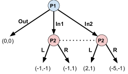
	L	R
Out	0,0	0,0
In1	-1,-1	-1,1
In2	2,1	-5,-1

Figure 1: In1 is strictly dominated by Out but provides the same information as In2 and performs better than In2 against some P2 strategies.

The strategy In1 is strictly dominated by Out for P1, and the iterated-dominance criterion of [23] requires that “A solution of a game $G$ contains a solution of any game $G^{\prime}$ obtained from $G$ by deletion of a dominated strategy.” In the game $G^{\prime}$ that results from the deletion of In1, $(\textbf{In2},\textbf{L})$ is the only sequential equilibrium and so the only strategically stable equilibrium. Thus the Nash equilibrium $(\textbf{Out},\textbf{In1})$ is ruled out by forward induction.

In contrast, when an inexperienced P1 agent plays this game and observes the terminal node at the each of each match, the agent may find it optimal to play In1. This is because In1 and In2 are informationally equivalent experiments: they provide the same signal about how P2s play. But if P1’s current belief puts much higher probability on P2s playing R than L, then P1’s expected payoff from In1 exceeds that of In2. A sufficiently patient P1 agent will choose to experiment and learn about P2’s play in order to figure out whether Out or In2 is a better response against the aggregate P2 play, but the cheapest such experiment may be In1.

Claim 1.

$(\textbf{Out},\textbf{R})$ is a patiently stable strategy profile for the game in Figure 1.

In Section 5.1 we establish more general sufficient conditions for patient stability in two-player games where each player moves at most once. These conditions give us a class of games where patiently stable profiles fail forward induction because of the informational value of dominated strategies. The idea of the proof is to choose “supportive” priors that lead the early mover to experiment in a way consistent with the desired equilibrium (such as choosing In1 instead of In2 in the example above) unless they have previously seen an out-of-equilibrium response from the second mover.

3.1.2 Insufficient Data to Eliminate Weakly Dominated Opponent Play

In the previous example, there is a dominated strategy that is still used by a rational agent as it provides information about their opponents’ aggregate play. By contrast, for the game in Figure 2, the strategy In2 is doubly dominated by In1 for P2 agents: it provides the same information about opponent play but, whenever these actions can be played, In2 always gives a strictly lower payoff than In1. A rational P2 agent will therefore never play In2 even as an experiment, which makes it more surprising that the learning outcome for patient and long-lived agents can select a profile where P1 and P2 are deterred from entering by P3’s R, which is strictly inferior to L against In1.

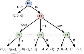
Figure 2: A three-player game where the strategy In2 is doubly dominated by In1 for P2. The dotted lines connecting two terminal nodes represent P2’s terminal node partition.

Here we suppose that P1 and P3 always observe the terminal node, but P2’s terminal node partition is such that they do not learn how P3 plays if they choose Out. Note that once the doubly dominated In2 is deleted for P2, L is a strictly better strategy than R for P3 against any strictly mixed play of P1 and P2. But:

Claim 2.

$(\textbf{Out},\textbf{Out},\textbf{R})$ is a patiently stable strategy profile for the game in Figure 2.

The presence of a third player is critical to this conclusion. The idea is that although aggregate P2 play puts zero probability on In2 (as required by the elimination of weakly dominated strategies) and positive probability on In1, a P3 agent may not have enough data to learn this aggregate play, as P3s only observe a P2 agent entering when they encounter both a P1 and a P2 agent experimenting with some In action. The incentive for P2 to experiment is weak because they are located off the equilibrium path and do not expect to play often, as in [20]. As a result, most P3 agents will never obtain any data to correct a prior belief that says it is more likely for P2’s to choose In2 than In1, so they find it optimal to play R. Even though the aggregate steady-state play of the P2s puts zero probability on the weakly dominated strategy, most P3s fail to learn this. We formally analyze this example in Section 5.2.

Invariance

The refinements literature following [23] argues that the selected set of equilibria should only depend on the normal form, so that any two extensive forms with the same normal form generate the same predictions. [23] say that this follows from the fact that the normal form “captures all the relevant information for decision purposes…” To this we would add “for fixed beliefs about the play of the opponents.” Simply splitting a decision node for one player, without changing any of the information sets of the opponents, does not change what any player observes either during the game or at the end of it, and so has no effect on the patiently stable outcomes, as in the following example.

In Figure 3, both games have the same set of patiently stable profiles (by Claim 3 below), but the outcome Out is only a sequential equilibrium outcome in the extensive form on the left.

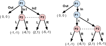
Figure 3: Both games have the same set of patiently stable profiles. But Out is only a sequential equilibrium outcome for the game on the left.

More generally, suppose extensive form $\hat{\mathcal{G}}$ is obtained by coalescing two consecutive information sets $h_{i}^{{}^{\prime}}$ and $h_{i}^{{}^{\prime\prime}}$ of $i$ in $\mathcal{G}$ into one information set $h_{i}^{\star}$ in $\hat{\mathcal{G}}$ (according to [9]’s “COA” definition of coalescence, as in Figure 4). Then they must have the same set of patiently stable profiles.

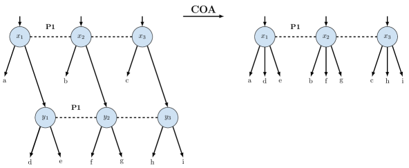
Figure 4: The coalesce operation is applied to two information sets of P1: $\{x_{1},x_{2},x_{3}\}$ and $\{y_{1},y_{2},y_{3}\}$.

Claim 3.

If $\mathcal{G}$ and $\hat{\mathcal{G}}$ are related by coalescing $h_{i}^{{}^{\prime}}$ and $h_{i}^{{}^{\prime\prime}}$ into $h_{i}^{\star}$, then they have the same set of patiently stable profiles (up to identifying $i$’s two actions at $h_{i}^{{}^{\prime}}$ and $h_{i}^{{}^{\prime\prime}}$ in $\mathcal{G}$ with their one action at $h_{i}^{\star}$ in $\hat{\mathcal{G}}$.)

When two information sets of $i$ are coalesced, the domain of $-i$’s prior beliefs about $i$’s play must be modified so that they are about $i$’s single action at the combined information set. Appendix A.1 gives the proof of Claim 3, which establishes a bijection between non-doctrinaire prior densities $g$ in the game $\mathcal{G}$ and $\hat{g}$ in the game $\hat{\mathcal{G}}$, so that the set of steady states are the same under $g$ in $\mathcal{G}$ and $\hat{g}$ in the $\hat{\mathcal{G}}$ for any $0\leq\delta,\gamma<1$.

However, other transformations of extensive form that leave the normal form unchanged can change the feedback players obtain in the course of play and so change the set of patiently stable outcomes.

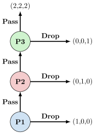
Pass

	Pass	Drop
Pass	2,2,2	0,1,0
Drop	1,0,0	1,0,0

Drop

	Pass	Drop
Pass	0,0,1	0,1,0
Drop	1,0,0	1,0,0

Figure 5: The two games have the same normal form, and (Pass, Pass, Pass) is the unique backward-induction profile for the extensive form on the left. (Drop, Drop, Pass) is patiently stable for the game on the left, but not for the game on the right.

As an example, compare the two games in Figure 5. In the game on the left, the unique backwards induction outcome is (Pass, Pass, Pass), but we know from [20] that the outcome (Drop, Drop, Pass) is also patiently stable: in the steady state, the P2s play so rarely that they choose not to experiment with Pass and so never learn that the P3s Pass. But this outcome is ruled out when agents play the normal form.

Claim 4.

Suppose agents play the normal form on the right of Figure 5 and observe opponents’ strategies at the end of each match. Then the only patiently stable outcome is (Pass, Pass, Pass).

This claims follows from Proposition 4 that we discuss later in Section 6.1. In the game on the right of Figure 5, P3s always Pass because they have full-support beliefs about what others do. Unlike for the game on the left, now P2s do not need to experiment to learn this. Once P2s learn that P3s play Pass, they themselves play Pass. This means that, when agents are long-lived, the vast majority of P2s in the population play Pass, so P1s learn to play Pass over Drop as well.

As these examples suggest, the problem is that the normal form does not distinguish between extensive forms that differ in what is observable during the learning process. We should only expect the set of learning outcomes to be invariant to transformations that are both decision invariant, i.e., lead to the same best responses as a function of opponent strategies, and information invariant in the sense of providing the same feedback to the agents in their learning problems. In the example above, this can be done by augmenting the normal form with the terminal node partition shown in Figure 6.

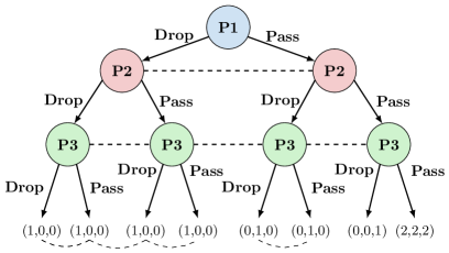
Figure 6: The game on the right of Figure 5 equipped with terminal node partitions. This game provides the same feedback to players as the game on the left of Figure 5.

The partition, which is common to all three players, says that if P1 plays Drop, players do not observe the choices of P2 and P3, and that if P1 plays Pass and P2 plays Drop then they do not observe the choice of P3. Under this partition, (Drop, Drop, Pass) again becomes patiently stable. Section 6 discusses how the terminal node partitions influence which profiles are patiently stable.

The Learning Model

There is a unit mass population of agents who play each role $1\leq i\leq I$ in the game. In every period, each agent is anonymously matched with opponents from the other populations uniformly at random to play the stage game. At the end of each play of the game, each agent observes the element of their terminal node partition $\mathcal{P}_{i}$ that contains the realized terminal node of the game, where we require that $u_{i}(z)=u_{i}(z^{\prime})$ if $z$ and $z^{\prime}$ are in the same cell of $i$’s terminal node partition. The agent uses this information to update their beliefs about the distribution of play in opponent populations.

As in [11] and [6], we assume that the agents have geometrically distributed lifetimes: At the end of every period, each agent exits the system with probability $0<1-\gamma\leq 1$, and a mass of newcomers is added to each population to replace the departing agents. Agents maximize expected discounted utility, discounting future payoffs with a psychological discount factor $0\leq\delta<1$.

Denote the set of pure strategies of $i$ in the game as $\mathbb{S}_{i}$ and the set of behavior strategies of $i$ as $\Pi_{i}$. Agents believe that the aggregate distribution of play in the opponent population is constant, but they do not know what that distribution is. Each agent in population $i$ starts with a prior belief $g_{i}\in\Delta(\times_{h\in\mathcal{H}_{-i}}\Delta(A_{h}))$ about the aggregate behavior strategy profile that describes play in opponent populations $j\neq i$ at different information sets. We assume that, for each $i$, the prior $g_{i}$ is non-doctrinaire, meaning that it has a density which is strictly positive on the interior of $\times_{h\in\mathcal{H}_{-i}}\Delta(A_{h})$.

As agents play the game and accumulate histories of past play and observations, they update their beliefs using Bayes’ rule (which is always applicable because the priors assign positive probability to any finite sequence of observations) and modify their behavior. Let $Y_{i,t}=(\mathbb{S}_{i}\times\mathcal{P}_{i})^{t}$ be the set of possible histories that can be observed by an $i$ agent of age $t$. (By convention, $\Omega^{0}=\emptyset$ for any set $\Omega$.) Let $Y_{i}=\cup_{t\in\mathbb{N}}Y_{i,t}$ be the collection of all possible histories of agents from population $i$. We assume that all agents in each population $i$ use the same optimal dynamic policy $\mathbf{s}_{i}^{\delta,\gamma}:Y_{i}\to\mathbb{S}_{i}$ that depends on both their discount factor, $\delta$, and their lifetime parameter $\gamma$.

In every period $t$, the state of the system, denoted $\mu_{t}=(\mu_{1,t},...,\mu_{I,t})\in\times_{i}\Delta(Y_{i})$, gives the shares of agents in the different player roles with the various possible histories. Given $\mu_{t}$, the player $i$ policy $\mathbf{s}_{i}^{\delta,\gamma}$ induces a player $i$ behavior strategy $\mathbf{\sigma}_{i}^{\delta,\gamma}(\mu_{i,t})\in\Pi_{i}$ that we call the aggregate strategy of population $i$. We call $\mathbf{\sigma}^{\delta,\gamma}(\mu_{t})=(\mathbf{\sigma}_{i}^{\delta,\gamma}(\mu_{i,t}))_{i}\in\times_{i}\Pi_{i}$ the aggregate strategy profile.

A policy profile generates an update rule $\mathbf{f}^{\delta,\gamma}:\times_{i}\Delta(Y_{i})\rightarrow\times_{i}\Delta(Y_{i})$, taking the state in period $t$ to the state in period $t+1$, and the mappings $\mathscr{R}_{i}^{\delta,\gamma}:\Pi_{-i}\rightarrow\Pi_{i}$ that describes the limit of the aggregate $i$ strategy as $t\rightarrow\infty$ when the aggregate $-i$ strategy is fixed at $\pi_{-i}$. We refer to the mapping $\mathscr{R}^{\delta,\gamma}(\pi)\equiv(\mathscr{R}_{1}^{\delta,\gamma_{1}}(\pi_{-1}),...,\mathscr{R}_{I}^{\delta,\gamma}(\pi_{-I}))$ as the aggregate response mapping. Similar arguments to those in [6] show that this mapping is continuous.

We study this system’s steady states, those $\mu$ satisfying $\mathbf{f}^{\delta,\gamma}(\mu)=\mu$. We call the corresponding aggregate strategy profiles the steady state profiles, and denote them by $\Pi^{*}(g,\delta,\gamma)\subseteq\times_{1\leq i\leq I}\Pi_{i}$. Again, similar arguments to those in [6] show that these are the fixed points of the aggregate response mapping. Continuity of the aggregate response mapping, along with Brouwer’s fixed point theorem, then implies that steady state profiles always exist.

Proposition 1.

$\Pi^{*}(g,\delta,\gamma)$ consists of the strategy profiles that are fixed points of the aggregate response mapping, and it is non-empty for all $g$, $\delta$, and $\gamma$.

When the agents are short-lived they have little chance to learn, and simply play a best response to their priors. When agents are long-lived but impatient, they do learn the steady state path of play, but need not learn how opponents respond to deviations, so any self-confirming equilibrium in strategies that are not weakly dominated could arise. We will focus on steady states where agents are both long-lived and patient. More specifically, we focus on steady state profiles in the limit where agents become long lived ($\gamma\rightarrow 1$) and patient ($\delta\rightarrow 1$). Moreover, following the literature, we assume continuation probability $\gamma$ converges to $1$ faster than $\delta$. We call these the patiently stable strategy profiles. The order of limits corresponds to an environment where agents are long-lived relative to their effective discount factors. This implies that people spend most of their lives myopically responding to their current beliefs.

Definition 1.

Strategy profile $\pi$ is patiently stable if there are sequences $\{\delta_{j}\}_{j\in\mathbb{N}}$, $\{\gamma_{j,k}\}_{j,k\in\mathbb{N}}$ and associated steady-state profiles $\{\pi_{j,k}\in\Pi^{*}(g,\delta_{j},\gamma_{j,k})\}_{j,k\in\mathbb{N}}$ such that $\lim_{j\rightarrow\infty}\delta_{j}=1$, $\lim_{k\rightarrow\infty}\gamma_{j,k}=1$ for each $j$ and $\lim_{j\rightarrow\infty}\lim_{k\rightarrow\infty}\pi_{j,k}=\pi$.

The literature has previously shown that patiently stable strategy profiles must be Nash equilibria when agents observe the realized terminal nodes in the games they play.

Appendix A.2 shows that this is also true for the game and terminal node partition given in Figure 2, which is the only example in the paper that uses a non-discrete terminal node partition to exhibit a patiently stable profile that is ruled out by classic refinements. We conjecture that patiently stable profiles must be Nash equilibria in any game provided each agent’s payoff is measurable with respect to their terminal node partition, but we have not shown this. Instead, Appendix A.3 gives a number of other examples from the literature where this conclusion does hold.

Patient Stability, Forward Induction, and Dominance

Dominated Actions in a Family of Two-Player Games

This section provides a sufficient condition for patient stability that generalizes the example from Section 3.1.1. We consider a family of two-player games where P1 first chooses an action $a_{1}\in A_{1}$, which may end the game or give the play to P2. For each P2 information set $h_{2}$, P2 chooses among the actions $\mathcal{A}_{2}(h_{2})$, and we let $\rho(h_{2})$ denote the P1 actions that lead to $h_{2}$. Write $u_{i}(a_{1},a_{2})$ for $i$’s utility at the terminal node reached by P1 playing $a_{1}$ and P2 playing $a_{2}$. We also write $u_{i}(\pi_{1},\pi_{2})$ for $i$’s expected utility when players use behavior strategies $\pi_{1}$ and $\pi_{2}$.

We will show that equilibria of the following form are patiently stable under some non-doctrinaire prior that we construct.

1. P1 plays a single action $a_{1}^{*}\in A_{1}$ that uniquely maximizes their payoff given P2’s strategy. (Formally, $\pi_{1}^{*}(a_{1}^{*})=1$ for the $a_{1}^{*}$ that satisfies $u_{1}(a_{1}^{*},\pi_{2}^{*})>u_{1}(a_{1},\pi_{2}^{*})$ for all $a_{1}\neq a_{1}^{*}$.)

2. For each P2 information set $h_{2}$, P2 plays some response $a_{2}^{*}(h_{2})$ that is optimal given some $a_{1}^{*}(h_{2})\in\rho(h_{2})$. Moreover, out of $\rho(h_{2})$, $a_{1}^{*}(h_{2})$ is optimal for P1 given that P2 plays $a_{2}^{*}(h_{2})$.

3. If $a^{*}_{1}$ leads to P2 information set $h_{2}^{*}$, then $a_{2}^{*}(h_{2}^{*})$ uniquely maximizes P2’s payoff against $a_{1}^{*}$.

The $(\textbf{Out},\textbf{In2})$ equilibrium from Section 3.1.1 is of this form: Out serves the role of $a_{1}^{*}$, and for P2’s only information set, P2’s prescribed response of R is the unique best response to In1. In turn, In1 is the best action out of $\{\textbf{In1},\textbf{In2}\}$ for P1 when P2 chooses R.

In the equilibria we construct, P2 may best reply to dominated P1 actions $a_{1}^{*}(h_{2})$ at some information sets $h_{2}$. Nevertheless, we show in Proposition 2 below that every such equilibrium is patiently stable, which implies Claim 1.

Proposition 2.

Suppose that $\pi^{*}$ is an equilibrium of the form given above. Then $\pi^{*}$ is patiently stable for any pair of non-doctrinaire P1 and P2 priors that are supportive of $\pi^{*}$.

The key is to choose priors that are “supportive” of the equilibrium. A supportive P1 prior is such that, for every off-path P2 information set $h_{2}$, a P1 agent prefers to experiment with $a_{1}^{*}(h_{2})$ over any other action in $\rho(h_{2})$ unless they have previously experienced a P2 response at $h_{2}$ for which $a_{1}^{*}(h_{2})$ is not conditionally optimal. Similarly, a supportive P2 prior leads P2 agents to want to play $a_{2}^{*}(h_{2})$ at an information set $h_{2}$ unless they have previously witnessed a P1 agent play some action in $\rho(h_{2})$ other than $a_{1}^{*}(h_{2})$. These properties are formalized in Appendix A.4, which also contains the proof of Proposition 2.

Stability and Doubly Dominated Actions: An Example

The example from Section 3.1.2 does not fit with the sufficient conditions for stability we gave in Section 5.1: it involves P3 best replying to the action In2 by P2, a doubly dominated action that is not optimal among the P2 actions $\{$In1,In2$\}$ that reach the same P3 information set. We use a different argument to show that the $(\textbf{Out},\textbf{Out},\textbf{R})$ outcome is patiently stable.

Proposition 3.

For the game in Figure 2, (Out, Out, R) is a patiently stable profile for any non-doctrinaire P1 prior $g_{1}$, non-doctrinaire P2 prior $g_{2}$ under which the expected probability of L is strictly less than $1/2$, and non-doctrinaire P3 prior $g_{3}$ that leads a P3 agent to only play L when they have previously observed a P2 agent play In1.

This proposition specifies the prior beliefs that make patient stability hold in Claim 2. The proof of this result in Appendix A.5 first notes that P1 observes P3’s play if and only if they experiment with In. This lets us bound the number of periods that P1s will typically experiment with In before becoming pessimistic and switching to Out forever in a steady state where P3s play R with high enough probability, so most P2 agents will learn that their information set is rarely reached. Thus they will choose Out instead of experimenting with In1, since they do not value information they will rarely get to use. This lets us construct a steady state where most P3 agents have never observed any instance of matched P2 agents choosing any action other than Out, and therefore choose R based on their prior belief.

Observability and Patiently Stable Profiles

In this section, we study the effect of what agents observe at the end of each play of the game on the patiently stable profiles. Sections 6.1 and 6.2 show that in normal forms arising from simple games, where agents always observe matched opponents’ extensive-form strategies, patiently stable profiles must select the same outcome as the backward induction outcome of the original game. Section 6.3 says that if the normal form of an extensive form is equipped with the right terminal node partitions, it leads to the same patiently stable profiles as the extensive form. Section 6.4 provides an example where patiently stable profiles satisfy the iterated deletion of weakly dominated strategies with coarser observations but not finer ones.

Backward Induction in Simple Games when Agents Observe Strategies

A simple game is an extensive-form game of perfect information where no one moves more than once along any path and no player is indifferent between any two terminal nodes, so there exists a unique backward induction strategy profile.

Consider the normal form of the simple game where agents simultaneously choose strategies from the extensive-form game tree and observe opponents’ strategies at the end of the match. The next result shows that the only patiently stable profile of the normal form is the backward induction strategy profile. In fact, we show something stronger: this is the only profile that is $\delta$-stable.

Definition 2.

For $0\leq\delta<1$ and non-doctrinaire prior $g$, strategy profile $\pi$ is $\mathbf{\delta}$-stable under $g$ if there is a collection of parameter sequences $\{\gamma_{k}\}_{k\in\mathbb{N}}$ and associated steady-state profiles $\{\pi_{k}\in\Pi^{*}(g,\delta,\gamma_{k})\}_{k\in\mathbb{N}}$ such that $\lim_{k\rightarrow\infty}\gamma_{k}=1$ and $\lim_{k\rightarrow\infty}\pi_{k}=\pi$.

Proposition 4.

Suppose agents play the normal-form representation of a simple game. Then, every $\delta$-stable profile puts probability $1$ on a backward-induction outcome.

In particular, this implies that for the normal form in Figure 5, (Pass, Pass, Pass) is the only learning outcome when agents are sufficiently long lived. As we show in Appendix A.7, Proposition 4 follows from a more general result in the next section about patient stability in normal form games.

An Iterative Deletion Refinement in Normal Forms

The next proposition discusses the implications of patient stability in environments of “maximal observability”: that is, agents play the normal form derived from an extensive form game and observe their opponents’ strategies. This result gives us a benchmark of what long-lived agents will learn in games if they do not need to experiment. The result takes the form of an iterative procedure that eliminates at each step some of the remaining strategies that do not best respond to strictly mixed conjectures that put arbitrarily low conditional probabilities on eliminated opponent strategies. Let $\mathcal{S}=\{\times_{i}\widetilde{S}_{i}:\forall i,\leavevmode\nobreak\ \widetilde{S}_{i}\subseteq S_{i}\}$ be the set of product spaces generated by the subsets of the player strategy spaces.

Definition 3.

A sequence $(S^{(0)},D^{(0)}),(S^{(1)},D^{(1)})...\in\mathcal{S}^{2}$ is a valid elimination sequence if

1. For each $i$, $S_{i}^{(0)}=S_{i}\setminus D_{i}^{(0)},$ and $D_{i}^{(0)}$ is any subset of $i$’s weakly dominated strategies,

2. For each $i$ and $m>0$, $D_{i}^{(m)}$ is a subset of $S_{i}^{(m-1)}$ such that, for every $s_{i}\in D_{i}^{(m)}$, there exists some $\epsilon>0$ where $\mathbb{E}_{\sigma_{-i}}[u_{i}(s_{i},s_{-i})]<\max_{s_{i}^{\prime}\in S_{i}}\mathbb{E}_{\sigma_{-i}}[u_{i}(s_{i}^{\prime},s_{-i})]$ for all correlated opponent strategy profiles $\sigma_{-i}\in\Delta(S_{-i})$ satisfying $\sigma_{-i}(S_{j}^{(m-1)}|s_{-ij})\geq 1-\epsilon$ for every $j\neq i$ and $s_{-ij}\in S_{-ij}$, and

3. For each $i$ and $m>0$, $S_{i}^{(m)}=S_{i}^{(m-1)}\backslash D_{i}^{(m)}.$

In a valid elimination sequence, at every stage of the iteration, the only player $i$ strategies that can be eliminated are those for which the following condition holds: There is an $\epsilon>0$ such that the strategy is suboptimal under any conjecture that, for each opponent $j$, puts probability at least $1-\epsilon$ on $j$ strategies that have not yet been eliminated conditional on any strategy profile of the opponents other than $j$.

Proposition 5.

For a valid elimination sequence $(S^{(0)},D^{(0)}),(S^{(1)},D^{(1)})...\in\mathcal{S}^{2}$, let $S_{i}^{*}=\cap_{m=0}^{\infty}S_{i}^{(m)}$. If agents observe matched opponents’ strategy choices at the end of each game, then every $\delta$-stable strategy profile is supported on the non-empty set $\times_{i}S_{i}^{*}$.

The idea behind the proof is that agents never use weakly dominated strategies in $D_{i}^{(0)}$ because they have full-support beliefs about others’ play, and experienced agents learn that these strategies are rarely used by an extension of [8]’s result in [17]. This implies strategies in $D_{i}^{(1)}$ only get used with very low probabilities in the steady state, as they are only played by the very young agents. Iterating this argument lets us eliminate the strategies in $D_{i}^{(2)},D_{i}^{(3)}$, and so forth.

Different valid elimination sequences may lead to different strategy sets $S_{i}^{*}$ in the end. Proposition 5, which we prove in Appendix A.6 gives a family of necessary conditions of patient stability, corresponding to different valid elimination sequences.

Some of the valid elimination sequences correspond to well-known solution concepts. One example is backward induction in simple games: Proposition 4 follows from Proposition 5 by letting $D_{i}^{(m)}$ be those extensive-form strategies of $i$ that are inconsistent with backward induction at some decision node $m+1$ steps away from the terminal nodes, but agree with it at all decision nodes $m$ or fewer steps away from the terminal nodes. The proof of Proposition 4 verifies that these $D_{i}^{(m)}$ form a valid elimination sequence.

A second example is the solution concept $S^{\infty}W$ ([7]), which [2] shows is equivalent to players having full support beliefs about the play of others and that this and the rationality of the players are “almost common knowledge.” This solution concept corresponds to choosing $D_{i}^{(0)}$ to be all weakly dominated strategies of $i$ in the original game, and, at each step $m,$ choosing $D_{i}^{(m+1)}\subseteq S_{i}^{(m)}$ to be the strictly dominated strategies of $i$ in the reduced game where $i$ has the strategy set $S_{i}^{(m)}.$ To see that this is a valid elimination sequence, note that if $s_{i}$ is strictly dominated, then there is some $\sigma_{i}\in\Delta(S_{i}^{(m)})$ and $\eta>0$ so that $u_{i}(\sigma_{i},s_{-i})>u_{i}(s_{i},s_{-i})+\eta$ for all $s_{-i}\in S_{-i}^{(m)}.$ By continuity, there exists some $\epsilon>0$ so that for any full-support correlated opponent strategy $\sigma_{-i}$ of the original game where $\sigma_{-i}(S_{-i}^{(m)})\geq 1-\epsilon$, we have $u_{i}(\sigma_{i},\sigma_{-i})>u_{i}(s_{i},\sigma_{-i})+\eta/2$, so in particular $s_{i}$ is not a best response to any such $\sigma_{-i}$.

While the refinement in Proposition 5 is stronger than $S^{\infty}W$, it is weaker than iterated elimination of weakly dominated strategies. This is because in defining $D_{i}^{(m)}$ in the iterative procedure, we consider conjectures where the probabilities assigned to deleted strategies can be arbitrarily small, but need not be zero. Provided there are at least two remaining strategies, this does not imply that the highest probability assigned to a deleted strategy must be lower than the lowest probability assigned to a remaining strategy. This distinguishes the Proposition 5 refinement from other refinement concepts like the iterated admissibility of [4] and the consistent pairs of [3]. For instance, for the game in Figure 7, there is no valid elimination sequence that uniquely selects the (A, X) strategy profile, even though (A, X) is the unique iteratively admissible profile. From a learning perspective, the idea is that although C is strictly dominated for P1, if P1 always play B then P2 can still maintain a belief that C is relatively more likely than A and thus choose Y. Indeed, it is easy to see that (B, Y) is a steady-state profile for any $0\leq\delta,\gamma<1$ (and therefore, patiently stable) if P1 starts with a strong prior belief that P2s play Y and P2s start with a Dirichlet prior with weights (1, 1, 10) on the P1 actions (A, B, C).

	X	Y
A	2, 2	0, 0
B	1, 1	1, 1
C	-10, 0	-10, 1

Figure 7: In this game, (A, X) is the unique iteratively admissible outcome [4], but (B, Y) is also patiently stable.

Information-Equivalent Normal Forms

For an extensive form $\mathcal{G}$ and terminal node partitions $\mathcal{P}$, consider the normal form $\mathcal{N}$ whose terminal nodes correspond to strategy profiles in $\mathcal{G},$ that is $\times_{i}\mathbb{S}_{i}$. Learning from the terminal node partition $\mathcal{P}$ in $\mathcal{G}$ and learning in $\mathcal{N}$ (with the standard assumption that the normal-form strategies played are observed by all the players at the end of each game) lead to different patiently stable profiles in general, as shown above. However, when $\mathcal{N}$ is equipped with the appropriate terminal node partitions, it will have the same set of patiently stable profiles as $\mathcal{G}$.

The $\mathcal{P}-$equivalent terminal node partitions are $\mathcal{\hat{P}}_{i}$ for $i$ in $\mathcal{N}$ are such that $\mathcal{\hat{P}}_{i}(s)=\mathcal{\hat{P}}_{i}(s^{\prime})$ if and only if $\mathcal{P}_{i}(\mathbf{z}(s))=\mathcal{P}_{i}(\mathbf{z}(s^{\prime}))$. Players hold beliefs over opponents’ behavior strategies in $\mathcal{G}$ and mixed strategies in $\mathcal{N}$, but we can transform a non-doctrinaire belief over behavior strategies into one over mixed strategies and vice versa when $\mathcal{G}$ has perfect recall, by Kuhn’s theorem.

Proposition 6.

The patiently stable profiles of $(\mathcal{G},\mathcal{P})$ are the same as the patiently stable profiles of $\mathcal{N}$ with the $\mathcal{P}-$equivalent terminal node partitions.

Intuitively, the definition of $\mathcal{\hat{P}}_{i}$ implies agents have the same feedback in the two games, so the problems are information invariant, and the normal form and extensive form are decision invariant. We formally show this in Appendix A.8.

Coarser Terminal Partitions May Eliminate Patiently Stable Profiles

Sections 6.1 and 6.2 show that coarser observations of opponents’ strategies can expand the set of patiently stable profiles. But this is not always true, and coarser terminal node partitions can shrink rather than expand the set of patiently stable profiles in other games.

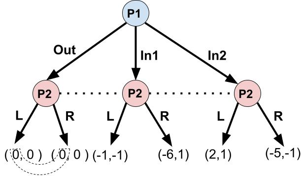
Figure 8: In the game on the left, both players observe the terminal node. In the game on the right, P1 does not observe P2’s play if they choose Out. The (Out, R) profile is patiently stable for the game on the left, but not for the game on the right.

Consider the two games in Figure 8 that only differ in the terminal node partition of P1. In the game on the left with the finer terminal node partitions, (Out, R) is patiently stable. It is easy to see that if P1 and P2 both start with a strong prior belief in the (Out, R) equilibrium and P2 thinks In1 is more likely than In2 when they have only seen P1s play Out, then it is a steady state under any $0\leq\delta,\gamma<1$ for (Out, R) to be played in every match.

But, (Out, R) is not patiently stable in the game on the right with the coarser terminal node partitions, as we show in Claim 5. The proof idea, which we rigorously demonstrate in Appendix A.9, is that patient P1 players will spend many periods experimenting with In2, since they cannot learn P2’s play by choosing Out. This teaches P2s that P1s are much more likely to use In2 than In1, so that they should not play R.

Claim 5.

For the game on the right in Figure 8, suppose P2’s prior belief satisfies Condition $\mathcal{P}$ from [14]. Then, every patiently stable profile satisfies $\pi(R)=0.$

Note that In1 is strictly dominated for P1, and if P2 thinks that P1 never plays In1, then L is strictly better than R for P2 given any conjecture that puts positive probabilities on both Out and In2. Thus (Out, R) is ruled out by iterated elimination of weakly dominated strategies, and stable learning outcomes in the example violate this refinement with a finer terminal node partition, but not with a coarser one.

Conclusion

The implications of learning depend crucially on the structure of the game and on what agents observe about others’ play. When the game and the feedback structure make it profitable for patient players to experiment with dominated strategies (for instance, when agents get no information from choosing a safe action but can use a worse safe action to learn about the consequences of a risky action), patiently stable profiles may violate forward induction or iterated weak dominance. When agents must experiment to learn about off-path play, patiently stable profiles may violate backward induction. But if agents observe opponents’ strategies regardless of their own play, patiently stable profiles always satisfy backward induction in simple games. This shows that ruling out some Nash equilibria requires close attention to the details of the game and the learning environment.

As in previous work, we have assumed that agents have non-doctrinaire priors in order to appeal to the [8] result on the speed of convergence of Bayesian posteriors to the empirical distribution. [17] extends their convergence result to priors without full support, but if the true state is outside of the support of the priors then agents need not stop experimenting in finite time, as shown by [21]. This raises a suite of new issues, as patiently stable states might not be Nash equilibria.

Also, the assumption that agents have non-doctrinaire priors over aggregate play in the other populations rules out settings where agents place probability $0$ on opponent strategies that they believe are strictly dominated. Since much of the refinements literature implicitly assumes all players know the payoff functions of the others, it is natural to wonder if adding some forms of restrictions on the priors would bring the patiently stable outcomes closer to the predictions of classic equilibrium refinements. In the case of signaling games with independent priors, [12] shows that the answer is “yes,” but the implications of payoff information in general games are unclear. One issue is that, as we have seen, agents may choose to use dominated strategies for their information value, and an agent whose prior gave these strategies probability $0$ would be unable to form a Bayesian posterior. Of course, this problem does not arise with myopic players, for they will never pay a current cost to obtain information. But with myopic players there is no reason to expect learning to lead to a Nash equilibrium, let alone a refinement of it.

Appendix

Appendix A Omitted Proofs

Proof of Claim 3

Suppose we have $A_{h_{i}^{{}^{\prime}}}=\{a_{1},...,a_{m},a_{\text{pass}}\}$ with the action $a_{\text{pass}}$ leading to $h_{i}^{\prime\prime}$, $A_{h_{i}^{\prime\prime}}=\{a_{m+1},...,a_{m+n}\}$, and $A_{h_{i}^{\star}}=\{a_{1},...,a_{m},a_{m+1},...,a_{m+n}\}.$ (For example, in Figure 4, $m=1$ and $n=2$.) Let $\Delta^{\circ}(X)$ the distributions on $X$ that assign strictly positive probability to each very element in $X.$ We define $\phi:\Delta^{\circ}(A_{h_{i}^{{}^{\prime}}})\times\Delta^{\circ}(A_{h_{i}^{\prime\prime}})\to\Delta^{\circ}(A_{h_{i}^{\star}})$, such that $\phi(\alpha_{h_{i}^{{}^{\prime}}},\alpha_{h_{i}^{{}^{\prime\prime}}})(a_{k})=\alpha_{h_{i}^{{}^{\prime}}}(a_{k})$ for $1\leq k\leq m$, while $\phi(\alpha_{h_{i}^{{}^{\prime}}},\alpha_{h_{i}^{{}^{\prime\prime}}})(a_{k})=\alpha_{h_{i}^{{}^{\prime}}}(a_{\text{pass}})\cdot\alpha_{h_{i}^{{}^{\prime\prime}}}(a_{k})$ for $m+1\leq k\leq m+n.$ That is, $\phi(\alpha_{h_{i}^{{}^{\prime}}},\alpha_{h_{i}^{{}^{\prime\prime}}})$ is a way to choose an element of $A_{h_{i}^{\star}}$ by using $\alpha_{h_{i}^{{}^{\prime}}}$ and $\alpha_{h_{i}^{{}^{\prime\prime}}}$ sequentially: first draw an element from $A_{h_{i}^{{}^{\prime}}}$ according to $\alpha_{h_{i}^{{}^{\prime}}}$ and then, if the chosen element is $a_{\text{pass}},$ draw an element from $A_{h_{i}^{{}^{\prime\prime}}}$ according to $\alpha_{h_{i}^{{}^{\prime\prime}}}.$ The map $\phi$ is one-to-one, because $\phi(\alpha_{h_{i}^{{}^{\prime}}},\alpha_{h_{i}^{{}^{\prime\prime}}})$ and $\phi(\beta_{h_{i}^{{}^{\prime}}},\beta_{h_{i}^{{}^{\prime\prime}}})$ generate different distributions on $\{a_{1},...,a_{m})$ if $\alpha_{h_{i}^{{}^{\prime}}}\neq\beta_{h_{i}^{{}^{\prime}}}$, while $\phi(\alpha_{h_{i}^{{}^{\prime}}},\alpha_{h_{i}^{{}^{\prime\prime}}})$ and $\phi(\alpha_{h_{i}^{{}^{\prime}}},\beta_{h_{i}^{{}^{\prime\prime}}})$ generate different distributions on $\{a_{m+1},...,a_{m+n}\}$ if $\alpha_{h_{i}^{{}^{\prime\prime}}}\neq\beta_{h_{i}^{{}^{\prime\prime}}}$ and $\alpha_{h_{i}^{{}^{\prime}}}$ a positive probability to $a_{\text{pass}}.$ Also, $\phi$ is onto, because for a given $\alpha_{h_{i}^{\star}}\in\Delta^{\circ}(A_{h_{i}^{\star}}),$ let $\alpha_{h_{i}^{\prime}}\in\Delta^{\circ}(A_{h_{i}^{{}^{\prime}}})$ be such that $\alpha_{h_{i}^{\prime}}(a_{k})=\alpha_{h_{i}^{\star}}(a_{k})$ for $1\leq k\leq m$, $\alpha_{h_{i}^{\prime}}(a_{\text{pass}})=1-\sum_{k=1}^{m}\alpha_{h_{i}^{\star}}(a_{k}),$ and $\alpha_{h_{i}^{\prime\prime}}(a_{k})=\frac{\alpha_{h_{i}^{\star}}(a_{k})}{\sum_{j=m+1}^{m+n}\alpha_{h_{i}^{\star}}(a_{j})}$ for $m+1\leq k\leq m+n.$ It is clear that by construction, $\phi(\alpha_{h_{i}^{\prime}},\alpha_{h_{i}^{\prime\prime}})=\alpha_{h_{i}^{\star}}.$ We have $\phi(\alpha_{h_{i}^{{}^{\prime}}},\alpha_{h_{i}^{{}^{\prime\prime}}})=\alpha_{h_{i}^{\star}}$ if and only if $(\alpha_{h_{i}^{{}^{\prime}}},\alpha_{h_{i}^{{}^{\prime\prime}}})$ and $\alpha_{h_{i}^{\star}}$ generate the same choice probabilities over the final actions $\{a_{1},...,a_{m},a_{m+1},...,a_{m+n}\}.$

For each agent $j$ in game $\mathcal{G}$, let $g_{j}:\times_{h\in\mathcal{H}_{-j}}\Delta(A_{h})\to\mathbb{R}_{+}$ be $j$’s prior prior density over $-j$’s strategies. Let $\hat{\mathcal{H}}_{i}$ represent $i$’s information sets in $\hat{\mathcal{G}}$, and continue to use $\mathcal{H}_{j}$ for $j$’s information sets in $\hat{\mathcal{G}}$ for agents $j\neq i.$ Let $\hat{g}_{j}:\times_{h\in\mathcal{\hat{H}}_{-j}}\Delta(A_{h})\to\mathbb{R}_{+}$ be a density of $j$’s belief about $-j$’s play in $\hat{\mathcal{G}}$ such that (1) if $j\neq i,$ then $\hat{g}_{j}(\alpha_{h_{i}^{\star}},(\alpha_{h})_{h\in\mathcal{\hat{H}}_{-j}\backslash\{h_{i}^{\star}\}})=g_{j}(\phi^{-1}(\alpha_{h_{i}^{\star}}),(\alpha_{h})_{h\in\mathcal{H}_{-j}\backslash\{h_{i}^{\prime},h_{i}^{\prime\prime}\}})/(\phi^{-1}(\alpha_{h_{i}^{\star}})(a_{\text{pass}}))^{n-1}$ for all strictly mixed actions $\alpha_{h_{i}^{\star}},(\alpha_{h})_{h\in\mathcal{\hat{H}}_{-j}\backslash\{h_{i}^{\star}\}}$; (2) for $i,$ $\hat{g}_{i}=g_{i}$. That is, $\hat{g}_{j}$ is over a different domain than $g_{j}$ since $i$ has one fewer information set in $\hat{\mathcal{G}}$ than $\mathcal{G},$ but we identify each strictly mixed $\alpha_{h_{i}^{\star}}$ in the domain of $\hat{g}_{j}$ with $\phi^{-1}(\alpha_{h_{i}^{\star}})$ in the domain of $g_{j}$ and re-normalize appropriately. Note $g_{j}$ is strictly positive on the interior and $0<\phi^{-1}(\alpha_{h_{i}^{\star}})(a_{\text{pass}})<\infty,$ so $\hat{g}_{j}$ is also strictly positive on the interior. This shows the constructed prior $\hat{g}$ is non-doctrinaire.

By the definition of $\phi$, each action in $\{a_{1},...,a_{m},a_{m+1},...,a_{m+n}\}$ has the same likelihood under $\alpha_{h_{i}^{\star}}$ and $\phi^{-1}(\alpha_{h_{i}^{\star}})$. Also, for every open set $E\subseteq\Delta^{\circ}(A_{h_{i}^{{}^{\prime}}})\times\Delta^{\circ}(A_{h_{i}^{\prime\prime}})$, the probability that $g_{j}$ assigns to $E$ is the same as the probability that $\hat{g}_{j}$ assigns to $\phi(E)\subseteq\Delta^{\circ}(A_{h_{i}^{\star}}).$ Note that for each $\alpha_{h_{i}^{{}^{\prime}}}\in\Delta^{\circ}(A_{h_{i}^{{}^{\prime}}})$, the projection $E_{\alpha_{h_{i}^{{}^{\prime}}}}:=\{\alpha_{h_{i}^{{}^{\prime\prime}}}\in\Delta^{\circ}(A_{h_{i}^{\prime\prime}}):(\alpha_{h_{i}^{{}^{\prime}}},\alpha_{h_{i}^{{}^{\prime\prime}}})\in E\}$ can be viewed as a subset of $\Delta_{n}^{1}:=\{x_{m+1},...,x_{m+n-1}\geq 0\text{ s.t. }x_{m+1}+...+x_{m+n-1}\leq 1\}\subseteq\mathbb{R}^{n-1}$. On the other hand, the image of this projection $\phi(\{\alpha_{h_{i}^{{}^{\prime}}}\}\times E_{\alpha_{h_{i}^{{}^{\prime}}}})$ can be viewed as a subset of $\Delta_{n}^{\alpha_{h_{i}^{{}^{\prime}}}(a_{\text{pass}})}:=\{x_{m+1},...,x_{m+n-1}\geq 0\text{ s.t. }x_{m+1}+...+x_{m+n-1}\leq\alpha_{h_{i}^{{}^{\prime}}}(a_{\text{pass}})\}\subseteq\mathbb{R}^{n-1}$. Both $\Delta_{n}^{1}$ and $\Delta_{n}^{\alpha_{h_{i}^{{}^{\prime}}}(a_{\text{pass}})}$ are $n-1$ dimensional polytopes, and the latter’s volume is $(\alpha_{h_{i}^{{}^{\prime}}}(a_{\text{pass}}))^{n-1}$ that of the former. The normalizing factor $1/(\phi^{-1}(\alpha_{h_{i}^{\star}})(a_{\text{pass}}))^{n-1}$ ensures $g_{j}(E)=\hat{g}_{j}(\phi(E))$,

Combining the two observations in the previous paragraph, we see that no matter which terminal node is observed, the posterior of $g_{j}$ will again assign the same probability to $E$ as the posterior of $\hat{g}_{j}$ assigns to $\phi(E).$ This discussion shows that for any $0\leq\delta,\gamma<1,$ the set of steady states with $\hat{g}$ in $\hat{\mathcal{G}}$ is the same as the set of steady states with $g$ in $\mathcal{G}$.

Conversely, given a prior density $\hat{g}_{j}$ for every agent $j$ in the game $\hat{\mathcal{G}}$, we can consider a prior density $g_{j}$ in $\mathcal{G}$ where $g_{j}(\alpha_{h_{i}^{{}^{\prime}}},\alpha_{h_{i}^{{}^{\prime\prime}}},(\alpha_{h})_{h\in\mathcal{H}_{-j}\backslash\{h_{i}^{\prime},h_{i}^{\prime\prime}\}})=\hat{g}_{j}(\phi(\alpha_{h_{i}^{{}^{\prime}}},\alpha_{h_{i}^{{}^{\prime\prime}}}),(\alpha_{h})_{h\in\mathcal{\hat{H}}_{-j}\backslash\{h_{i}^{\star}\}})\cdot(\alpha_{h_{i}^{{}^{\prime}}}(a_{\text{pass}}))^{n-1}$ for $j\neq i.$ The same argument as above shows for any $0\leq\delta,\gamma<1,$ the set of steady states with $g$ in $\mathcal{G}$ is the same as the set of steady states with $\hat{g}$ in $\hat{\mathcal{G}}$.

Patiently Stable Profiles for Figure 2 Are Nash Equilibria

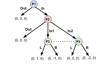
Figure 9: A game with fully revealing terminal node partitions in which the learning problem of a P2 agent with a given prior is identical to the learning problem of a P2 agent with the same prior in the Figure 2 game.

Proof.

Consider the auxiliary game depicted in Figure 9, which modifies payoffs to make P1 and P3 indifferent between all terminal nodes, and ends the game immediately if P2 chooses Out. For any $0\leq\delta,\gamma<1$, any P1 or P3 policy used in the original steady state is an optimal policy for the corresponding agent in the auxiliary game, so any steady state profile $\pi^{*}\in\Pi^{*}(g,\delta,\gamma)$ for the original game is also a steady state profile of the auxiliary game. And P2 faces the same learning problem in the auxiliary game as in the original game, since each strategy profile gives them the same payoff and the same feedback in both games. But we know in every patiently stable profile in the auxiliary game, P2 must not have a profitable deviation, so the same must apply to the patiently stable profiles of the original game. Likewise, we can construct auxiliary games for P1 and P3 to show that they must not have profitable deviations in patiently stable profiles of the original game. ∎

Examples of Games with Terminal Node Partitions That Have Auxiliary Games with Discrete Partitions

The argument in the previous section can be used to show that patient stability selects only Nash equilibria whenever the game and feedback structure are such that, for each player role, there is an auxiliary game with a discrete terminal node partition that leads to the same learning problem for agents in that role. We give some examples of games from the previous literature that meet this condition below.

In [15], Figure 1 Game B and Figure 3 present two games where three players P1, P2, and P3 simultaneously choose actions, P2 and P3 always see the terminal node, and P1 sees the terminal node when they choose In but not when they choose Out. P1 always gets 0 payoff from choosing Out. For P2 and P3, consider the auxiliary game where every player always observes the terminal node. This clearly does not affect P2 and P3’s learning problems. For P1, consider an auxiliary game where P1 moves first and the game ends with P1 getting 0 payoff if P1 chooses Out. If P1 chooses In, then P2 and P3 choose their actions simultaneously as before. All players observe terminal nodes. P1’s learning problem in the auxiliary game is the same as in the original game. Thus for Figure 1 Game B and Figure 3 with their original terminal node partitions, patiently stable profiles are Nash equilibria.

Figure 5 of [15] is a three-player game where P1, P2 and P3 simultaneously choose In or Out. When P1 chooses In, they learn P2 and P3’s choices, but P1 does not learn how others play if they choose Out. P2 always learns how P1 plays, but they only learn how P3 plays if they choose In rather than Out. Similarly, P3 always learns how P1 plays, but they only learn how P2 plays if they choose In rather than Out. Players who choose Out always get 0. For P1, consider the auxiliary game where they move first and choose In or Out. If they choose Out, the game ends with them getting 0. If they choose In, then P2 and P3 simultaneously choose In or Out. All players observe terminal nodes. This is the same learning problem as in the original game for P1. Next, consider the auxiliary game where P1 and P2 move simultaneously at the start of the game. If P2 chooses Out, the game ends with P2 getting 0. If P2 chooses In, then P3 chooses between In or Out without knowing P1’s choice. All players observe terminal nodes. This is the same learning problem as in the original game for P2, because the terminal node always reveals P1’s play, even when P2 chooses Out. But if P2 chooses Out, then the terminal node does not show what P3 would have played. Similarly, we can construct an analogous auxiliary game for P3. This shows that for the game in Figure 5, patiently stable profiles are Nash equilibria.

Section 5.1.1 of [13] studies the “restaurant game” where three players P1, P2, and P3 move simultaneously. P1 is a restaurant that chooses between high and low ingredient qualities, while P2 and P3 are two potential customers who decide whether to go to the restaurant (In) or eat at home (Out). P1 always sees P2 and P3’s choices. P2 sees how others play if they choose In, but not if they choose Out. Similarly, P3 sees how others play if they choose In, but not if they choose Out. Choosing Out always gives 0 payoff. For P1, the auxiliary game where everyone sees the terminal node does not affect their learning problem. For P2, consider the auxiliary game where they move first, choosing between In and Out. If they choose Out, the game ends with payoff 0 for them. If they choose In, then P1 and P3 move simultaneously. All players observe terminal nodes. This auxiliary game presents the same learning problem for P2 as in the original game. Similarly, there is an analogous auxiliary game with discrete terminal node partitions that preserves P3’s learning problem, so patiently stable profiles are Nash equilibria in this game.

Proof of Proposition 2

We first formally define supportive priors that are used to facilitate the proof.

Definition 4.

Priors $g_{1}$ and $g_{2}$ are supportive priors for $\pi^{*}$ if, for every off-path P2 information set $h_{2}$, (1) $\mathbb{E}_{g_{1}}[u_{1}(a_{1}^{*}(h_{2}),a_{2}(h_{2}))|y_{1}]\geq\mathbb{E}_{g_{1}}[u_{1}(a_{1},a_{2}(h_{2}))|y_{1}]$ for all $a_{1}\in\rho(h_{2})$ and P1 histories $y_{1}$ that have never recorded a P2 agent play some action other than $a_{2}^{*}(h_{2})$ at $h_{2}$, and (2) $\mathbb{E}_{g_{2}}[u_{2}(a_{1},a_{2}^{*}(h_{2}))|y_{2},h_{2}]\geq\mathbb{E}_{g_{2}}[u_{2}(a_{1},a_{2}))|y_{2},h_{2}]$ for all $a_{2}\in\mathcal{A}_{2}(h_{2})$ and histories $y_{2}$ that have never recorded a P1 agent play any $a_{1}\in\rho(h_{2})\backslash\{a_{1}^{*}(h_{2})\}$.

Proof of Proposition 2.

Throughout this proof, we think of P1 actions that end the game as leading to singleton P2 information sets where P2 only has one action. Denote the P2 information set reached when P1 plays $a_{1}^{*}$ with $h_{2}^{*}$, and use $\mathcal{H}_{2}^{off}=\mathcal{H}_{2}\setminus\{h_{2}^{*}\}$ to denote the set of P2 information sets that are off-path under $\pi^{*}$. Let $\widetilde{\Pi}_{1}=\{\pi_{1}\in\Pi_{1}:\forall h_{2}\in\mathcal{H}_{2}^{off},\leavevmode\nobreak\ \pi_{1}(a_{1})=0\leavevmode\nobreak\ \forall a_{1}\in\rho(h_{2})\setminus\{a_{1}^{*}(h_{2})\}\}$ be the set of P1 behavior strategies that, for every $h_{2}\in\mathcal{H}_{2}^{off}$, put probability $0$ on any action in $\rho(h_{2})$ that is not $a_{1}^{*}(\alpha_{1})$. Further, let $\widetilde{\Pi}_{2}=\{\pi_{2}\in\Pi_{2}:\forall h_{2}\in\mathcal{H}_{2}^{off},\leavevmode\nobreak\ \pi_{2}(a_{2}^{*}(h_{2})|h_{2})=1\}$ be the set of P2 behavior strategies which respond with $a_{2}^{*}(h_{2})$ at any off-path information set $h_{2}$. Throughout the proof, we restrict attention to strategy profiles $\pi\in\widetilde{\Pi}_{1}\times\widetilde{\Pi}_{2}$.

By continuity, there is an $\eta>0$ such that (1) for any $\pi_{1}\in\Pi_{1}$ satisfying $\pi_{1}(a_{1}^{*})\geq 1-\eta$, the unique optimal action for P2 to play at $h_{2}^{*}$ is $a_{2}^{*}(h_{2}^{*})$, and (2) for any $\pi_{2}\in\widetilde{\Pi}_{2}$ for which $\pi_{2}(a_{2}^{*}(h_{2}^{*})|h_{2}^{*})\geq 1-\eta$, the unique P1 best response is $a_{1}^{*}$. We focus on steady state profiles in which the aggregate probabilities that P1 plays $a_{1}^{*}$ and that P2 plays $a_{2}^{*}(h_{2}^{*})$ at $h_{2}^{*}$ both exceed $1-\eta$. We argue that such steady state profiles exist in the limit, and that the corresponding aggregate probabilities that P1 plays $a_{1}^{*}$ and P2 plays $a_{2}^{*}(h_{2})$ in response to any information set $h_{2}$ converge to $1$.

Let $\xi:\widetilde{\Pi}_{1}\rightarrow\widetilde{\Pi}_{1}$ be the continuous mapping given by

$$\xi(\pi_{1})(a_{1})=\begin{cases}\max\{\pi_{1}(a_{1}^{*}),1-\eta\}&\text{if }a_{1}=a_{1}^{*}\\ \left(1-\mathbbm{1}(\pi_{1}(a_{1}^{*})<1-\eta)\frac{1-\eta-\pi_{1}(a_{1}^{*})}{1-\pi_{1}(a_{1}^{*})}\right)\pi_{1}(a_{1})&\text{if }a_{1}\neq a_{1}^{*}\end{cases}.$$

This function transforms each $\pi_{1}$ into a P1 behavior strategy that puts probability at least $1-\eta$ on $a_{1}^{*}$ and satisfies $\xi(\pi_{1})=\pi_{1}$ whenever $\pi_{1}(a_{1}^{*})\geq 1-\eta$. Similarly, let $\phi:\widetilde{\Pi}_{2}\rightarrow\widetilde{\Pi}_{2}$ be the continuous mapping such that

$$\phi(\pi_{2})(a_{2}|h_{2}^{*})=\begin{cases}\max\{\pi_{2}(a_{2}^{*}(h_{2}^{*})|h_{2}^{*}),1-\eta\}&\text{if }a_{2}=a_{2}^{*}(h_{2}^{*})\\ \left(1-\mathbbm{1}(\pi_{2}(a_{2}^{*}(h_{2}^{*})|h_{2}^{*})<1-\eta)\frac{1-\eta-\pi_{2}(a_{2}^{*}(h_{2}^{*})|h_{2}^{*})}{1-\pi_{2}(a_{2}^{*}(h_{2}^{*})|h_{2}^{*})}\right)\pi_{2}(a_{2}|h_{2}^{*})&\text{if }a_{2}\neq a_{2}^{*}(h_{2}^{*})\end{cases}.$$

This takes each $\pi_{2}$ into a P2 behavior strategy that uses $a_{2}^{*}(h_{2}^{*})$ at $h_{2}^{*}$ with probability at least $1-\eta$. Note that $\phi$ coincides with the identity mapping whenever $\pi_{2}(a_{2}^{*}(h_{2}^{*})|h_{2}^{*})\geq 1-\eta$.

Since $g_{1}$ is supportive of $\pi^{*}$, for any $\pi_{2}\in\widetilde{\Pi}_{2}$, $\mathscr{R}_{1}^{\delta,\gamma}(\pi_{2})(a_{1})=0$ for all $a_{1}\in\rho(h_{2})$ for all $h_{2}\in\mathcal{H}_{2}^{off}$. This means that $\mathscr{R}_{1}^{\delta,\gamma}(\pi_{2})\in\widetilde{\Pi}_{1}$ for all $\pi_{2}\in\widetilde{\Pi}_{2}$. Likewise, since $g_{2}$ is supportive of $\pi^{*}$, for any $\pi_{1}\in\widetilde{\Pi}_{1}$, $\mathscr{R}_{2}^{\delta,\gamma}(\pi_{1})(a_{2}|h_{2})=0$ for all $a_{2}\neq a_{2}^{*}(h_{2})$ for all $h_{2}\in\mathcal{H}_{2}^{off}$. Thus, $\mathscr{R}_{2}^{\delta,\gamma}(\pi_{1})\in\widetilde{\Pi}_{2}$ for all $\pi_{1}\in\widetilde{\Pi}_{1}$. Consequently, $\mathscr{R}^{\delta,\gamma}$ maps $\widetilde{\Pi}_{1}\times\widetilde{\Pi}_{2}$ into itself regardless of $\delta,\gamma\in[0,1)$, so the mapping $\widetilde{\mathscr{R}}^{\delta,\gamma}:\widetilde{\Pi}_{1}\times\widetilde{\Pi}_{2}\rightarrow\widetilde{\Pi}_{1}\times\widetilde{\Pi}_{2}$ given by $\widetilde{\mathscr{R}}^{\delta,\gamma}(\pi_{1},\pi_{2})=(\xi(\mathscr{R}_{1}^{\delta,\gamma}(\pi_{2})),\phi(\mathscr{R}_{2}^{\delta,\gamma}(\pi_{1})))$ is well-defined. Since this mapping is continuous, Brouwer’s fixed point theorem guarantees the existence of a fixed point $\pi^{\delta,\gamma}=(\pi_{1}^{\delta,\gamma},\pi_{2}^{\delta,\gamma})$ for any $\delta,\gamma\in[0,1)$.

Consider some arbitrary collection of parameter sequences $\{\delta_{j}\}_{j\in\mathbb{N}}$, $\{\gamma_{j,k}\}_{j,k\in\mathbb{N}}$ such that $\lim_{j\rightarrow\infty}\delta_{j}=1$, $\lim_{k\rightarrow\infty}\gamma_{j,k}=1$ for all $j\in\mathbb{N}$, and $\lim_{j\rightarrow\infty}\lim_{k\rightarrow\infty}\pi^{\delta_{j},\gamma_{j,k}}=\hat{\pi}$ for some $\hat{\pi}\in\widetilde{\Pi}_{1}\times\widetilde{\Pi}_{2}$. Using the fact that the unique P1 best response is $a_{1}^{*}$ to any $\pi_{2}\in\widetilde{\Pi}_{2}$, $\lim_{j\rightarrow\infty}\lim_{k\rightarrow\infty}\mathscr{R}_{1}^{\delta_{j},\gamma_{j,k}}(\pi_{2}^{\delta_{j},\gamma_{j,k}})(a_{1}^{*})=1$ can be shown using a similar auxiliary game argument to the one given when arguing that patient stability selects Nash equilibria in the Figure 2 game. Thus, $\lim_{j\rightarrow\infty}\lim_{k\rightarrow\infty}\mathscr{R}_{1}^{\delta_{j},\gamma_{j,k}}(\pi_{2}^{\delta_{j},\gamma_{j,k}})=\pi_{1}^{*}$. As $\xi(\pi_{1})=\pi_{1}$ if $\pi_{1}(a_{1}^{*})\geq 1-\eta$, it follows that $\mathscr{R}_{1}^{\delta_{j},\gamma_{j,k}}(\pi_{2}^{\delta_{j},\gamma_{j,k}})=\pi_{1}^{\delta_{j},\gamma_{j,k}}$ whenever $j$ is sufficiently large and $k$ is sufficiently large given $j$. Similarly, since $a_{2}^{*}(h_{2}^{*})$ is the uniquely optimal action to use at $h_{2}^{*}$ given any $\pi_{1}\in\widetilde{\Pi}_{1}$, $\lim_{j\rightarrow\infty}\lim_{k\rightarrow\infty}\mathscr{R}_{2}^{\gamma_{j,k}}(\pi_{1}^{\delta_{j},\gamma_{j,k}})(a_{2}^{*}(h_{2}^{*})|h_{2}^{*})=1$ must hold. This means that $\lim_{j\rightarrow\infty}\lim_{k\rightarrow\infty}\mathscr{R}_{2}^{\gamma_{j,k}}(\pi_{1}^{\delta_{j},\gamma_{j,k}})=\pi_{2}^{*}$. Moreover, as $\phi(\pi_{2})=\pi_{2}$ if $\pi_{2}(a_{2}^{*}(h_{2}^{*})|h_{2}^{*})\geq 1-\eta$, it follows that $\mathscr{R}_{2}^{\delta_{j},\gamma_{j,k}}(\pi_{1}^{\delta_{j},\gamma_{j,k}})=\pi_{2}^{\delta_{j},\gamma_{j,k}}$ whenever $j$ is sufficiently large and $k$ is sufficiently large given $j$. Collecting these findings reveals that $\pi^{\delta_{j},\gamma_{j,k}}$ is a fixed point of the aggregate response mapping $\mathscr{R}^{\delta_{j},\gamma_{j,k}}$, and thus a steady state profile by Proposition 1, whenever $j$ is sufficiently large and $k$ is sufficiently large given $j$. Since $\lim_{j\rightarrow\infty}\lim_{k\rightarrow\infty}\pi^{\delta_{j},\gamma_{j,k}}=\pi^{*}$, we conclude that $\pi^{*}$ is stable. ∎

Proof of Proposition 3

We first establish three lemmas.

Lemma 1.

Fix $\delta\in[0,1)$ and a non-doctrinaire P1 prior $g_{1}$. For each $\gamma\in[0,1)$, fix a P1 policy that is optimal given $g_{1}$ and never prescribes In after it has previously prescribed Out. There is some $\kappa\in\mathbb{R}_{+}$ such that, for arbitrary $\gamma\in[0,1)$, when the aggregate P3 strategy puts probability $\pi_{3}^{\delta,\gamma}(\textbf{L})\leq 1/4$ on L, the aggregate P1 strategy satisfies $\pi_{1}^{\delta,\gamma}(\textbf{In})/(1-\gamma)\leq\kappa$.

Proof.

We first establish that there is some $N\in\mathbb{N}$ such that all P1 agents who have lived at $t\geq N$ periods and have been matched with P3 agents that would play L fewer than $t/3$ periods would play Out. By Theorem 4.2 of [8], there is an $N\in\mathbb{N}$ such that a P1 agent who has played In at least $N$ times and for whom, when they have played In, the share of times they have observed their P3 opponent play R is at least $2/3$, will put probability at least $3/(4-\delta)$ on the true probability with which a randomly selected P3 agent plays R being weakly more than $2/3$. Such an agent thus puts at least probability $3/(4-\delta)$ on aggregate opponent behavior strategy profiles for which the expected payoff from playing In is no more than $-1/3$. This $N$ satisfies the desired properties given at the beginning of the paragraph. To see this, consider a P1 agent who has lived at least $N$ periods and for whom the fraction of time periods where they were matched with a P3 agent that would play L that periods is less than $1/3$. Then, either that agent has played Out in the past, in which case they will again play Out, or that agent has actually observed the consequences of playing In at least $N$ times. Restricting attention to the latter case, the agent must have a posterior belief that puts probability $p>3/(4-\delta)$ on aggregate opponent behavior strategy profiles for which the expected payoff from playing In is no more than $-1/3$. An upper bound on the agent’s expected discounted future lifetime payoff from playing In is $(1-\delta)(1-4p/3)+\delta(1-p)$, since the expected current period payoff to playing In is weakly less than $p(-1/3)+1-p=1-4p/3$ and the agent’s continuation payoff is bounded above by $\delta(1-p)$, since P1’s maximum payoff is $1$. As $p>3/(4-\delta)$, it follows that $(1-\delta)(1-4p/3)+\delta(1-p)<0$, so such an agent must play Out.

We now combine this fact with Hoeffding’s inequality to derive the desired constraint on the P1 aggregate strategy. By Hoeffding’s inequality, there is some $c>0$ such that, for any aggregate P3 strategy satisfying $\pi_{3}^{\delta,\gamma}(\textbf{L})\leq 1/4$, the share of P1 agents who have lived $n$ periods and for whom the fraction of time periods where they were matched with a P3 agent that would play L is less than $1/3$ is at least $1-e^{-cn}$. Thus, we have that

$$\begin{split}\frac{\pi_{1}^{\delta,\gamma}(\textbf{In})}{1-\gamma}&\leq\frac{1}{1-\gamma}\left(1-\gamma^{N}+\sum_{t=N}^{\infty}(1-\gamma)\gamma^{t}e^{-ct}\right)\\ &=\frac{1-\gamma^{N}}{1-\gamma}+\frac{\gamma^{N}e^{-cN}}{1-\gamma e^{-c}}.\end{split}$$

Observe that the right-hand side of the inequality converges to $N+1/(e^{cN}-e^{c(N-1)})$ as $\gamma\rightarrow 1$. Since $\pi_{1}^{\delta,\gamma}(\textbf{In})/(1-\gamma)$ can never be more than $1/(1-\gamma)$, it follows that $\pi_{1}^{\delta,\gamma}(\textbf{In})/(1-\gamma)$ must be uniformly bounded from above by some $\kappa\in\mathbb{R}_{+}$. ∎

Lemma 2.

Fix $\delta\in[0,1)$ and a non-doctrinaire P2 prior $g_{2}$ under which the expected probability of L is strictly less than $1/2$. Consider a sequence of steady states such that the probability of In under the aggregate P1 strategy satisfies $\pi_{1}^{\delta,\gamma}(\textbf{In})/(1-\gamma)\leq\kappa$ for all $\gamma\in[0,1)$ for some $\kappa\in\mathbb{R}_{+}$. Then $\lim_{\gamma\rightarrow 1}\pi_{2}^{\delta,\gamma}(\textbf{Out})=1$.

Proof.

Fix an $\epsilon>0$ such that the expected probability of L under $g_{2}$ is weakly less than $(1-\epsilon)/2$. We first establish that there is some $N_{0}\in\mathbb{N}$ such that, regardless of $\gamma\in[0,1)$, every P2 agent who has lived at least $N_{0}$ periods and has never observed a P1 agent play In will play Out. Theorem 4.2 of [8] implies that there is an $N\in\mathbb{N}$ such that, under the posterior belief of a P2 agent who has at least $N$ observations of P1 agents playing Out and no observations of a P1 agent playing In, the expected value of the probability with which a randomly selected P1 agent will play In, $\nu$, is strictly less than $(1-\delta)\epsilon/\delta$. This $N$ satisfies the desired properties given at the beginning of the paragraph. To see this, consider a P2 agent who has lived at least $N$ periods and has never observed a P1 agent play In. An upper bound on the agent’s expected discounted future lifetime payoff from playing In1 is $-(1-\delta)\epsilon+\delta\nu$, which is strictly negative since $\nu<(1-\delta)\epsilon/\delta$, so such an agent must play Out.

Inductively applying similar arguments to the one given above shows that there is a sequence of $\{N_{j}\}_{j\in\mathbb{N}}\subseteq\mathbb{N}$ such that the following holds. For all $\gamma\in[0,1)$ and $j\in\mathbb{N}$, every P2 agent who has lived at least $N_{j}$ periods, has at most $j$ observations of P1 agents playing In, and witnessed no P1 agents playing In in their first $N_{j}$ observations will play Out. Observe that, when the probability of a randomly selected P1 agent playing In is $\pi_{1}(\textbf{In})$, the share of P2 agents who have lived at least $N_{j}+j$ periods and have exactly $j$ observations of P1 agents playing In, all of which came after their first $N_{j}$ periods, is

$$\begin{split}&\sum_{t=N_{j}+j}^{\infty}(1-\gamma)\gamma^{t}\frac{(t-N_{j})!}{(t-N_{j}-j)!j!}\pi_{1}^{\delta,\gamma}(\textbf{In})^{j}\left(1-\pi_{1}^{\delta,\gamma}(\textbf{In})\right)^{t-j}\\ =&\gamma^{N_{j}+j}\left(1-\pi_{1}^{\delta,\gamma}(\textbf{In})\right)^{N_{j}}\frac{\pi_{1}^{\delta,\gamma}(\textbf{In})^{j}}{\left(1-\gamma+\gamma\pi_{1}^{\delta,\gamma}(\textbf{In})\right)^{j+1}}\\ =&\gamma^{N_{j}+j}\left(1-\pi_{1}^{\delta,\gamma}(\textbf{In})\right)^{N_{j}}\left(\frac{1+\frac{\pi_{1}^{\delta,\gamma}(\textbf{In})}{1-\gamma}}{1+\gamma\frac{\pi_{1}^{\delta,\gamma}(\textbf{In})}{1-\gamma}}\right)^{j+1}\frac{\left(\frac{\pi_{1}^{\delta,\gamma}(\textbf{In})}{1-\gamma}\right)^{j}}{\left(1+\frac{\pi_{1}^{\delta,\gamma}(\textbf{In})}{1-\gamma}\right)^{j+1}}.\end{split}$$

It thus follows that, for a given $\gamma\in[0,1)$ and steady-state strategy profile,

$$\begin{split}\pi_{2}^{\delta,\gamma}(\textbf{Out})&\geq\sum_{j=0}^{\infty}\gamma^{N_{j}+j}\left(1-\pi_{1}^{\delta,\gamma}(\textbf{In})\right)^{N_{j}}\left(\frac{1+\frac{\pi_{1}^{\delta,\gamma}(\textbf{In})}{1-\gamma}}{1+\gamma\frac{\pi_{1}^{\delta,\gamma}(\textbf{In})}{1-\gamma}}\right)^{j+1}\frac{\left(\frac{\pi_{1}^{\delta,\gamma}(\textbf{In})}{1-\gamma}\right)^{j}}{\left(1+\frac{\pi_{1}^{\delta,\gamma}(\textbf{In})}{1-\gamma}\right)^{j+1}}\\ &=1-\sum_{j=0}^{\infty}\left(1-\gamma^{N_{j}+j}\left(1-\pi_{1}^{\delta,\gamma}(\textbf{In})\right)^{N_{j}}\left(\frac{1+\frac{\pi_{1}^{\delta,\gamma}(\textbf{In})}{1-\gamma}}{1+\gamma\frac{\pi_{1}^{\delta,\gamma}(\textbf{In})}{1-\gamma}}\right)^{j+1}\right)\frac{\left(\frac{\pi_{1}^{\delta,\gamma}(\textbf{In})}{1-\gamma}\right)^{j}}{\left(1+\frac{\pi_{1}^{\delta,\gamma}(\textbf{In})}{1-\gamma}\right)^{j+1}}\\ &\geq 1-\sum_{j=K+1}^{\infty}\frac{\left(\frac{\pi_{1}^{\delta,\gamma}(\textbf{In})}{1-\gamma}\right)^{j}}{\left(1+\frac{\pi_{1}^{\delta,\gamma}(\textbf{In})}{1-\gamma}\right)^{j+1}}\\ &\leavevmode\nobreak\ \leavevmode\nobreak\ -\sup\left\{1-\gamma^{N_{j}+j}\left(1-\pi_{1}^{\delta,\gamma}(\textbf{In})\right)^{N_{j}}\left(\frac{1+\frac{\pi_{1}^{\delta,\gamma}(\textbf{In})}{1-\gamma}}{1+\gamma\frac{\pi_{1}^{\delta,\gamma}(\textbf{In})}{1-\gamma}}\right)^{j+1}\right\}_{j\in\{0,1,...,K\}}\end{split}$$

for arbitrary $K\in\mathbb{N}$. Fix an arbitrary $\eta>0$ and take $K$ to be large enough so that $\sum_{j=K+1}^{\infty}\kappa^{j}/(1+\kappa)^{j+1}<\eta$. Then the right-hand side of the first line of the final inequality is greater than $1-\eta$ for all $\pi_{1}^{\delta,\gamma}(\textbf{In})/(1-\gamma)\leq\kappa$. Observe that the elements of the set over which the supremum is taken in the final line converge to $0$ as $\gamma\rightarrow 1$ uniformly over $\pi_{1}^{\delta,\gamma}(\textbf{In})/(1-\gamma)\leq\kappa$. Thus, $\liminf_{\gamma\rightarrow 1}\pi_{2}^{\delta,\gamma}(\textbf{Out})\geq 1-\eta$. Since this holds for all $\eta>0$, we have $\lim_{\gamma\rightarrow 1}\pi_{2}^{\delta,\gamma}(\textbf{Out})=1$. ∎

Lemma 3.

Fix $\delta\in[0,1)$ and a non-doctrinaire P3 prior $g_{3}$ that leads a P3 agent to only play L when they have previously observed a P2 agent play In1. Consider a sequence of steady-states such that the probability of In under the aggregate P1 strategy satisfies $\pi_{1}^{\delta,\gamma}(\textbf{In})/(1-\gamma)\leq\kappa$ for all $\gamma\in[0,1)$ for some $\kappa\in\mathbb{R}_{+}$ and $\lim_{\gamma\rightarrow 1}\pi_{2}^{\delta,\gamma}(\textbf{In1})=0$. Then $\lim_{\gamma\rightarrow 1}\pi_{3}^{\delta,\gamma}(\textbf{L})=0$.

Proof.

Observe that

$$\begin{split}\pi_{3}^{\delta,\gamma}(\textbf{L})&\leq\sum_{t=0}^{\infty}(1-\gamma)\gamma^{t}(1-(1-\pi_{1}^{\delta,\gamma}(\textbf{In})\pi_{2}^{\delta,\gamma}(\textbf{In1}))^{t})\\ &=1-\frac{1-\gamma}{1-\gamma(1-\pi_{1}^{\delta,\gamma}(\textbf{In})\pi_{2}^{\delta,\gamma}(\textbf{In1}))}\\ &=1-\frac{1}{1+\gamma\frac{\pi_{1}^{\delta,\gamma}(\textbf{In})}{1-\gamma}\pi_{2}^{\delta,\gamma}(\textbf{In1})}\end{split}$$

since the right-hand side of the inequality is the share of P3 agents who have previously observed a P2 agent play In1. By Lemma 1, there is some $\kappa\in\mathbb{R}_{+}$ such that $\limsup_{\gamma\rightarrow 1}\pi_{1}^{\delta,\gamma}/(1-\gamma)\leq\kappa$, while $\lim_{\gamma\rightarrow 1}\pi_{2}^{\delta,\gamma}(\textbf{In1})=0$ by Lemma 2. It follows that $\lim_{\gamma\rightarrow 1}1+\gamma(\pi_{1}^{\delta,\gamma}(\textbf{In}))/(1-\gamma)\pi_{2}^{\delta,\gamma}(\textbf{In1})=1$, which implies $\lim_{\gamma\rightarrow 1}\pi_{3}^{\delta,\gamma}(\textbf{L})=0$. ∎

Proof of Proposition 3.

Lemmas 1, 2, and 3 together imply that, for fixed $\delta\in[0,1)$, the aggregate response mapping maps the set of aggregate strategy profiles where $\pi_{3}^{\delta,\gamma}(L)\leq 1/4$ into itself when $\gamma$ is close enough to $1$. Brouwer’s fixed point theorem then guarantees the existence of a steady state profile satisfying this inequality for all sufficiently high $\gamma$. Lemmas 1, 2, and 3 further imply that, in the $\gamma\rightarrow 1$ limit of such a sequence of steady state profiles, $\lim_{\gamma\rightarrow 1}\pi_{1}^{\delta,\gamma}(\textbf{Out})=1$, $\lim_{\gamma\rightarrow 1}\pi_{2}^{\delta,\gamma}(\textbf{Out})=1$, and $\lim_{\gamma\rightarrow 1}\pi_{3}^{\delta,\gamma}(\textbf{R})=1$ must be satisfied. Since $\delta\in[0,1)$ is arbitrary, we conclude that $(\textbf{Out},\textbf{Out},\textbf{In})$ is patiently stable. ∎

Proof of Proposition 5

We first state a supporting lemma that shows that, with enough data, a given agent’s posterior beliefs will, for every opponent population, put high probability on the empirical distribution of strategies they have previously observed agents in that population use.

Lemma 4.

For any fixed non-doctrinaire prior and every $\eta>0$, there is some $M$ such that, whenever an agent has at least $M$ observations, for each opponent population, the agent’s posterior belief puts probability $1-\eta$ on strategy distributions within $\eta$, under the sup norm, of the empirical distribution they have observed.

This follows from the [17] extension of the pathwise concentration result of [8] to priors that do not have full support. The support restriction arise because the agent’s prior is concentrated on distributions that can be generated by independent randomizations of their opponents.

Proof of Proposition 5.

Fix a discount factor $\delta\in[0,1)$, and consider a sequence of survival probabilities $\{\gamma_{k}\}_{k=1}^{\infty}$ with an associated sequence of steady-state strategy profiles $\{\pi_{k}\}_{k=1}^{\infty}$ such that $\pi_{k}\to\pi^{*}$. We show that $\pi_{i}^{*}(s_{i})=0$ for each $i$ and each $s_{i}\notin S_{i}^{*}$.

First, it is clear that $\pi_{i}^{*}(s_{i})=0$ for each $i$ and each $s_{i}\notin S_{i}^{(0)}$. This is because agents have full-support posterior beliefs after every history and their observations do not depend on their play, so they never use weakly dominated strategies.

By Lemma 4, for a given $\eta>0$, there is some $M$ such that, whenever a player has at least $M$ observations, their posterior belief over the prevailing strategy distribution in each of their opponent populations puts probability $1-\eta$ on strategy distributions within $\eta$ of the empirical distribution they have observed. By the law of large numbers, we can choose this $M$ to be such that the posterior beliefs of an agent in an arbitrary player role $i$ who has lived at least $M$ periods will be accurate with high probability in the following sense. With probability $1-2\eta$, at the end of the period, following any possible observation in the period itself, the agent’s posterior belief puts probability at least $1-2\eta$ on strategy distributions within $2\eta$ of the true prevailing distribution for each opponent role $j\neq i$.

Now suppose inductively that $\pi_{i}^{*}(s_{i})=0$ for each $i$ and $s_{i}\notin S_{i}^{(m)}$ for some $m$. Fix arbitrary $\epsilon,\nu>0$ and restrict attention to $k$ large enough so that $|\pi_{i,k}-\pi_{i}^{*}|<\epsilon/2$ for all player roles $i$. By the preceding argument, we know that for all sufficiently large $k$, in a given period the share of player $i$ agents whose posterior beliefs at the end of the period, regardless of their observations during the period, for each opponent role $j$ put probability at least $1-\epsilon$ on strategy distributions within $1-\epsilon$ of $\Delta(S_{j}^{(m)})$ will exceed $1-\nu$. Let $\sigma\in\Delta(S_{-i})$ be the expectation held by such an agent about the play of their opponents in the current period. The properties of the agent’s beliefs imply that $\sigma$ is full support and that $\sigma(S_{j}^{(m)}|s_{-ij})\geq(1-\epsilon)^{2}$ for all $s_{-ij}\in S_{-ij}$. For all sufficiently small $\epsilon$, every $s_{i}\not\in S_{i}^{(m)}$ must be suboptimal for such an agent, so $\pi_{i}^{*}(s_{i})\leq\nu$ must hold for each $i$ and $s_{i}\notin S_{i}^{(m+1)}$. Since this is true for all $\nu>0$, we conclude that $\pi_{i}^{*}(s_{i})=0$ for each $i$ and $s_{i}\notin S_{i}^{(m+1)}$.

∎

Proof of Proposition 4

Proof.

Let $D_{i}^{(m)}$ be those extensive-form strategies of $i$ that choose an action inconsistent with backward induction at a decision node that is $m+1$ steps away from the terminal nodes, but do not do so at any decision nodes closer to the terminal nodes. To see these choices are valid for the iterative procedure, first note $D_{i}^{(0)}$ are weakly dominated for $i$: For any $s_{i}\in D_{i}^{(0)},$ consider a different strategy $s_{i}^{\prime}$ that changes one of the non-backward-induction actions at one of $i$’s decision nodes $h_{i}$ one step away from terminal nodes to a backward-induction action. Then $u_{i}(s_{i}^{\prime},s_{-i})\geq u_{i}(s_{i},s_{-i})$ for all $s_{-i}$. Moreover, there exists at least one $s_{-i}^{*}$ such that $h_{i}$ is reached (since the game is simple), so $u_{i}(s_{i}^{\prime},s_{-i}^{*})>u_{i}(s_{i},s_{-i}^{*}).$

By definition, $S_{i}^{(m)}$ are the strategies where $i$ uses the backward-induction action at all decision nodes $m+1$ steps or fewer away from terminal nodes. To see that each $s_{i}\in D_{i}^{(m+1)}$ fails to be a best response for $i$ to full-support conjectures of their opponents’ play that put high conditional probabilities on $S_{j}^{(m)}$ for each $j\neq i$, let $h_{i}$ be a decision node $m+2$ steps away from terminal nodes where $s_{i}$ does not choose the backward-induction action, and let $s_{i}^{\prime}$ be the strategy that only differs from $s_{i}$ in that $s_{i}^{\prime}$ by selecting a backward-induction action at $h_{i}.$ Let $J$ be the set of players who have decision nodes in the subgame starting at $h_{i}$, not counting $h_{i}$ itself. Because the game is simple, $i\notin J$. For the same reason, whether play reaches $h_{i}$ does not depend on the strategy of $i$ or the strategies of the players in $J$. Let $S_{-iJ}^{reach}\subseteq S_{-iJ}$ be the set of strategies of $-iJ$ that reach $h_{i}$.

For any $s_{-i}\in S_{-i}^{(m)},$ $i$’s payoff in the subgame starting at $h_{i}$ is strictly higher with $s_{i}^{\prime}$ than with $s_{i},$ which we write as $u_{i}(s_{i},s_{-i}\mid h_{i})<u_{i}(s_{i}^{\prime},s_{-i}\mid h_{i}).$ This uses the fact that $i$’s payoff in the subgame starting at $h_{i}$ only depends on $i$’s action at $h_{i}$ and on the strategies of players in $J$. Consider any strictly mixed profile $\sigma_{-i}$ where $\sigma_{-i}(S_{J}^{(m)}|s_{-iJ})\geq 1-\epsilon$ for each $s_{-iJ}\in S_{-iJ}$. When $-iJ$ choose a strategy profile in $S_{-iJ}^{reach}$, $i$’s payoff is equal to $i$’s payoff in the subgame starting at $h_{i}.$ When $-iJ$ choose a strategy outside of $S_{-iJ}^{reach}$, $i$ is indifferent between $s_{i}$ and $s_{i}^{\prime}.$ Therefore, $u_{i}(s_{i},\sigma_{-i})-u_{i}(s_{i}^{\prime},\sigma_{-i})=\sigma_{-i}(S_{-iJ}^{reach})\cdot[\mathbb{E}[u_{i}(s_{i},s_{-i}\mid h_{i})|S_{-iJ}^{reach}]-u_{i}(s_{i}^{\prime},s_{-i}\mid h_{i})|S_{-iJ}^{reach}]].$ We have $\sigma_{-iJ}(S_{-iJ}^{reach})>0$ since each opponent’s strategy is strictly mixed, and we have $u_{i}(s_{i},(\sigma_{j})_{j\in J}\mid h_{i})-u_{i}(s_{i}^{\prime},(\sigma_{j})_{j\in J}\mid h_{i})<0$ for all sufficiently small $\epsilon>0$. ∎

Proof of Proposition 6

Proof.

First note that for every non-doctrinaire prior $g$ over behavior strategies in $\mathcal{G},$ there is a non-doctrinaire prior $\hat{g}$ over mixed strategies in $\mathcal{G}$ that generates the same set of steady states for every $0\leq\delta,\gamma<1$. This is because each $-i$ behavior strategy $(\alpha_{h_{-i}})_{h_{-i}\in\mathcal{H}_{i}}$ is associated with an equivalent mixed strategy $\sigma_{-i}\in\Delta(\mathbb{S}_{-i}),$ defined by $\sigma_{-i}(s_{-i})=\times_{h_{-i}\in\mathcal{H}_{-i}}\alpha_{h_{-i}}(s_{-i}(h_{-i}))$ for each $s_{-i}\in\mathbb{S}_{-i}$. This association maps the interior of the set of behavior strategies onto the interior of the set of mixed strategies, so the non-doctrinaire $g_{i}$ generates a non-doctrinaire $\hat{g}_{i}$ over $-i$’s mixed strategies. Conversely, if we start with a non-doctrinaire prior $\hat{g}$ over mixed strategies in $\mathcal{G}$, then by applying Kuhn’s theorem in a game with perfect recall, we can identify a non-empty set of equivalent behavior strategies for every mixed strategy. Consider the prior $g_{i}$ over $-i$ behavior strategies where $i$ believes $-i$ first draw a mixed strategy $\sigma_{-i}$ according to $\hat{g}_{i}$, and then randomize uniformly over all behavior strategies equivalent to it. Then $g_{i}$ is strictly positive on the interior because $\hat{g}_{i}$ enjoys the same property.

Learning with a non-doctrinaire prior $\hat{g}$ over mixed strategies in $\mathcal{G}$ with terminal node partitions $\mathcal{P}$ and learning with the same $\hat{g}$ in $\mathcal{N}$ with the $\mathcal{P}$-equivalent partitions generate the same set of steady states for every $0\leq\delta,\gamma<1$. This is because both environments generate the same dynamic optimization problem for each agent: in both environments, they start with the same prior beliefs, receive the same payoffs for each strategy profile $(s_{i},s_{-i})$ played, and observe the same information (up to identifying elements of the $\mathcal{P}_{i}$ partition with those in the equivalent $\hat{\mathcal{P}}_{i}$ partition.) ∎

Proof of Claim 5

Proof.

Suppose there is a prior $g$ satisfying the hypotheses of the claim, parameters $\{\delta_{j}\}_{j\in\mathbb{N}},$ $\{\gamma_{j,k}\}_{j,k\in\mathbb{N}}$, and associated steady-state profiles $\{\pi_{j,k}\in\Pi^{*}(g,\delta_{j},\gamma_{j,k})\}$ such that $\lim_{j\to\infty}\delta_{j}=1,$ $\lim_{k\to\infty}\gamma_{j,k}=1$ for each $j$, and $\lim_{j\to\infty}\lim_{k\to\infty}\pi_{j,k}=\pi$.

For arbitrary $\epsilon>0$, we will show $\pi(\textbf{R})<2\epsilon$. The idea is to show that all P2 agents except the very young and those with unusual samples will have seen enough instances of P1 choosing In2 and no instance of P1 choosing Out as to play L at their information set.

By Proposition 1 from [14], there exists some $x\geq 1$ so that if a P2 agent has $n$ observations of P1’s play and in each of their observations P1 never chose In1, then their mean posterior probability of P1 choosing In1 is lower than $\frac{2x}{n+x}$. By Theorem 1 from [14], there exists $N\geq 1$ such that in any steady state $\hat{\pi}$ where $\hat{\pi}({\textbf{In2}})\geq q$, with probability at least $1-\epsilon$ a P2 agent with age at least $N/q$ will have a mean posterior belief of P1 playing In2 that is higher than $(1-\epsilon)q$.

Define the constant $K=\frac{16Nx}{\epsilon}$ and find some $\beta<1$ so that, whenever $\delta\geq\beta$ and $\gamma\geq\beta$, a P1 agent will always choose In2 in the first $K$ periods of life.

Consider any $j$ large enough so that $\delta_{j}\geq\beta$. For large $k$, using the fact that P1 agents experiment with In2 for at least $K$ periods, $\pi_{j,k}({\textbf{In2}})\geq(1+\gamma_{j,k}+...+\gamma_{j,k}^{K-1})\cdot(1-\gamma_{j,k})\geq\frac{1}{2}(1-\gamma_{j,k})\cdot K$. So, a P2 agent aged at least $\frac{N}{\frac{1}{2}(1-\gamma_{j,k})\cdot K}=(\frac{\epsilon}{2}\frac{1}{1-\gamma_{j,k}})\cdot\frac{1}{4\cdot x}$ has at least $1-\epsilon$ chance of believing that P1 plays In2 with probability at least $\frac{1}{4}(1-\gamma_{j,k})\cdot K$. This age is no larger than $\frac{\epsilon}{2}$ times the expected P2 lifespan, which contains at least $1-\epsilon$ fraction of the P2 population. Also, a P2 agent with age at least $\frac{\epsilon}{2}\frac{1}{1-\gamma_{j,k}}$ has a mean posterior belief about P1 playing In1 that is always smaller than $\frac{2x}{\frac{\epsilon}{2}\frac{1}{1-\gamma_{j,k}}+x}=\frac{2x(1-\gamma_{j,k})}{\frac{1}{2}\epsilon+(1-\gamma_{j,k})x}\leq\frac{4x}{\epsilon}(1-\gamma_{j,k})$. Taking the ratio of the mean posterior beliefs assigned to P1 playing In2 and In1, we get $\frac{\frac{1}{4}(1-\gamma_{j,k})\cdot K}{\frac{4x}{\epsilon}(1-\gamma_{j,k})}=\frac{1}{16}K\cdot\frac{\epsilon}{x}=N\geq 1.$

Therefore, except for a mass of smaller than $\epsilon$ of P2s younger than $\frac{\epsilon}{2}\cdot\frac{1}{1-\gamma_{j,k}}$ and another mass $\epsilon$ of P2s with unusual samples, P2s respond to In1 and In2 with L. This shows in the steady state with $\delta_{j}$ and $k$ large enough, $\pi_{j,k}(\textbf{R})<2\epsilon$. This implies also that $\lim_{k\to\infty}\pi_{j,k}(\textbf{R})<2\epsilon$ for all large enough $j,$ therefore $\pi(\textbf{R})<2\epsilon.$ ∎

References

- [1] J.. Banks and J. Sobel “Equilibrium selection in signaling games” In Econometrica 55, 1987, pp. 647–661
- [2] Tilman Börgers “Weak dominance and approximate common knowledge” In Journal of Economic Theory 64.1, 1994, pp. 265–276
- [3] Tilman Börgers and Larry Samuelson ““Cautious” utility maximization and iterated weak dominance” In International Journal of Game Theory 21.1, 1992, pp. 13–25
- [4] Adam Brandenburger, Amanda Friedenberg and H Jerome Keisler “Admissibility in games” In Econometrica 76.2 Wiley Online Library, 2008, pp. 307–352
- [5] I-K. Cho and D.. Kreps “Signaling games and stable equilibria” In Quarterly Journal of Economics 102, 1987, pp. 179–221
- [6] Daniel Clark and Drew Fudenberg “Justified communication equilibrium” In American Economic Review 111.9, 2021, pp. 3004–34
- [7] Eddie Dekel and Drew Fudenberg “Rational behavior with payoff uncertainty” In Journal of Economic Theory 52.2 Elsevier, 1990, pp. 243–267
- [8] P. Diaconis and D. Freedman “On the uniform consistency of Bayes estimates for multinomial probabilities” In Annals of Statistics 18, 1990, pp. 1317–1327
- [9] Susan Elmes and Philip J Reny “On the strategic equivalence of extensive form games” In Journal of Economic Theory 62.1 Elsevier, 1994, pp. 1–23
- [10] Ignacio Esponda “Rationalizable conjectural equilibrium: A framework for robust predictions” In Theoretical Economics 8, 2013, pp. 467–501
- [11] Drew Fudenberg and Kevin He “Learning and type compatibility in signaling games” In Econometrica 86.4 Wiley Online Library, 2018, pp. 1215–1255
- [12] Drew Fudenberg and Kevin He “Payoff information and learning in signaling games” In Games and Economic Behavior 120 Elsevier, 2020, pp. 96–120
- [13] Drew Fudenberg and Kevin He “Player-compatible learning and player-compatible equilibrium” In Journal of Economic Theory 194 Elsevier, 2021, pp. 105238
- [14] Drew Fudenberg, Kevin He and Lorens A Imhof “Bayesian posteriors for arbitrarily rare events” In Proceedings of the National Academy of Sciences 114.19 National Acad Sciences, 2017, pp. 4925–4929
- [15] Drew Fudenberg and Y. Kamada “Rationalizable partition-confirmed equilibrium” In Theoretical Economics 10, 2015, pp. 775–806
- [16] Drew Fudenberg and Y. Kamada “Rationalizable partition-confirmed equilibrium with heterogeneous beliefs” In Games and Economic Behavior 109, 2018, pp. 364–381
- [17] Drew Fudenberg, Giacomo Lanzani and Philipp Strack “Pathwise concentration bounds for Bayesian beliefs” In Working Paper, 2021
- [18] Drew Fudenberg and David K Levine “Self-confirming equilibrium” In Econometrica JSTOR, 1993, pp. 523–545
- [19] Drew Fudenberg and David K. Levine “Steady state learning and Nash equilibrium” In Econometrica 61, 1993, pp. 547–573
- [20] Drew Fudenberg and David K. Levine “Superstition and rational learning” In American Economic Review 96, 2006, pp. 630–651
- [21] Drew Fudenberg, Gleb Romanyuk and Philipp Strack “Active learning with a misspecified prior” In Theoretical Economics 12.3 Wiley Online Library, 2017, pp. 1155–1189
- [22] Srihari Govindan and Robert Wilson “On forward induction” In Econometrica 77.1 Wiley Online Library, 2009, pp. 1–28
- [23] E. Kohlberg and J-F. Mertens “On the strategic stability of equilibria” In Econometrica 54, 1986, pp. 1003–1037
- [24] George J. Mailath, Larry Samuelson and Jeroen M. Swinkels “Extensive form reasoning in normal form games” In Econometrica 61.2 [Wiley, Econometric Society], 1993, pp. 273–302
- [25] Ariel Rubinstein and Asher Wolinsky “Rationalizable conjectural equilibrium: between Nash and rationalizability” In Games and Economic Behavior 6.2 Elsevier, 1994, pp. 299–311
- [26] Sylvain Sorin “A note on repeated extensive games” In Games and Economic Behavior 9.1 Academic Press, 1995, pp. 116–123