BDG-Net: Boundary Distribution Guided Network for Accurate Polyp Segmentation
Abstract
Colorectal cancer (CRC) is one of the most common fatal cancer in the world. Polypectomy can effectively interrupt the progression of adenoma to adenocarcinoma. Colonoscopy is the primary method to find colonic polyps. However, due to the different sizes and the unclear boundary of polyps, it is challenging to segment polyps accurately. To this end, we design a Boundary Distribution Guided Network (BDG-Net) for accurate polyp segmentation. Specifically, Boundary Distribution Generate Module (BDGM) aggregates high-level features to generate Boundary Distribution Map (BDM), which is sent to the Boundary Distribution Guided Decoder (BDGD) as complementary spatial information to guide the polyp segmentation. Moreover, a multi-scale feature interaction strategy is adopted in BDGD to improve the polyps segmentation of different sizes. Extensive experiments demonstrate that BDG-Net outperforms state-of-the-art models remarkably and maintains low computational complexity. Code: https://github.com/zihuanqiu/BDG-Net
keywords:
Polyp segmentation, Colorectal cancer, Colonoscopy, Deep learning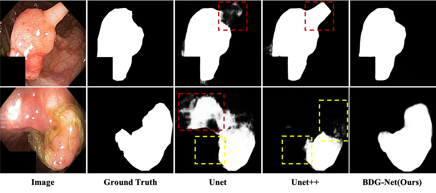 |
1 INTRODUCTION
Medical image segmentation is an essential part of the artificial intelligence-assisted diagnosis. It can provide some fine-grained information to assist diagnosis, such as the location and shape of the polyps. This information is critical and helpful for successful treatment, even preventing disease. Take colorectal cancer(CRC) as an example. CRC is the third most common type of cancer around the world[2]. Early detection through colonoscopy has been shown to be effective in reducing disease-related mortality.
Recently, the convolutional neural network (CNN) based medical image segmentation methods have achieved favorable performance in many datasets. Most of them are based on encoder-decoder structure. The most representative method is U-Net[3], which captures precise context with skip paths. Oktay et al.[4] introduced attention-mechanism to the segmentation network based on U-Net. Zhou et al.[5] proposed a variant of U-Net named UNet++, in which decoder sub-networks are connected by dense skip paths. PraNet[6] proposed reverse attention to achieve accurate polyp segmentation. However, due to the different sizes of polyps and the unclear boundary between polyps and their surrounding mucosa, segmentation models often suffer under-segmentation or over-segmentation, as shown in Figure 1.
In this paper, we propose a Boundary Distribution Guided Segmentation Network (BDG-Net), which consists of two novel modules. The first one is the Boundary Distribution Generate Module (BDGM), aggregating the high-level features and generating Boundary Distribution Map (BDM) under the supervision of the ideal BDM. The second one is the Boundary Distribution Guided Decoder (BDGD), which uses the generated BDM as complementary information, fusing different multi-scale features to improve polyp segmentation on different sizes. Quantitative and qualitative experiments show that our proposed model outperforms state-of-the-art methods on five challenging polyp datasets while maintaining low computational complexity.
The contributions of this work are summarized as follows:
-
(1)
We design BDGM to generate BDM, which can be used as complementary spatial information to guide the accurate polyp segmentation.
-
(2)
We propose BDGD, which fuses multi-scales features to improve polyp segmentation on different sizes.
-
(3)
Integrating the above two modules into a single architecture, we design BDG-Net, which outperforms state-of-the-art models remarkably on five challenging polyp datasets while maintaining low computational complexity.
2 Methodology
In this section, we first give the definition of our proposed BDM and then introduce our two modules, BDGM and BDGD, respectively. Next, we specify the loss function we used. Finally, the entire architecture of the proposed BDG-Net is described.
2.1 Boundary Distribution Map
Due to the unclear or illegible boundary of the polyps, it is challenging to clarify the polyps boundary accurately. However, it is much easier to estimate the range of the boundary. Based on this intuition, we propose BDM, which is a map representing the estimated probability that the current pixel belongs to the boundary. We assume that the boundary distribution follows a Gaussian distribution with a mean of 0 and a standard deviation of . The ideal BDM can be defined as follows:
| (1) |
where is the shortest Euclidean distance from pixel to the boundary and is the standard deviation.
 |
2.2 Boundary Distribution Generate Module
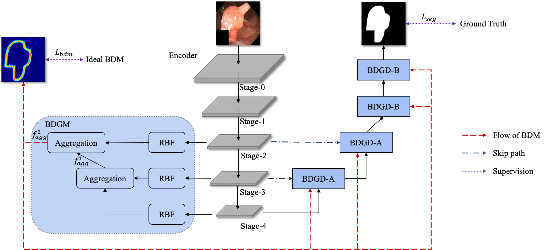
To predict the boundary distribution, we propose BDGM, which generates BDM under the supervision of the ideal BDM. BDGM aggregates the features from the last three stages of the encoder and gradually increases the feature resolution. As shown in Figure 2, we use the Receptive Field Block[7](RBF) to reduce the channel dimension of features and then aggregate the third and fourth-stage of encoder features to output , with resolution being (). Then the obtained feature is aggregated with the second-stage features, and the resolution of the output feature is (). Finally, we use bilinear interpolation to upsample by 8 to generate BDM.
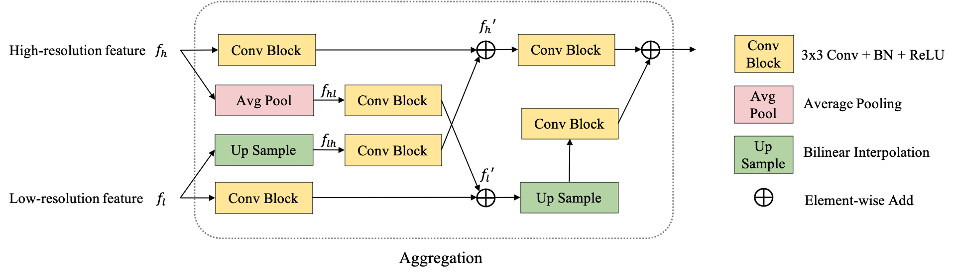
The aggregation is designed to maintain lightweight and efficient. As shown in Figure 3, the high-resolution feature is downsampled by average pooling to get , and the low-resolution feature is upsampled by bilinear interpolation to get . Then and go through 33 convolution followed by BN and ReLU to get and , respectively. The convoluted is added with to obtain feature . Similarly, The convoluted is added to to obtain feature . Finally, the upsampled goes through convolution block and adds with the convoluted to get the output feature. The aggregation operation can be denoted as follows:
| (2) | |||
| (3) | |||
| (4) |
where refers to convolutional layer with kernel size 3 followed by BN and ReLU. represents the upsampling by bilinear interpolation.
 |
2.3 Boundary Distribution Guided Decoder
 |
BDGD uses the BDM generated by BDGM to guide the model segment accurately. In the higher stages, we use BDGD-A, which takes the output of the previous decoder and the encoder features as input, obtaining sufficient spatial information by interacting with the features on two scales. Specifically, as shown in Figure 4(a), let be the encoder feature and be the output of the previous decoder. Note that the resolution of is two times larger than . Firstly, we transform and into output’s channel dimensions through convolutional layer and get and . Then, is multiplied by BDM, and is multiplied by the downsampled BDM, after which the boundary enhanced features and are obtained. The upsampled goes through a ConvBlock and adds with to get the high-resolution fused feature. The downsampled goes through a ConvBlock and adds with to get the low-resolution fused feature. Then the low-resolution fused feature is upsampled and added with the high-resolution fused feature to achieve cross-scale feature fusion. Finally, a residual structure is used to help optimization.
Similarly, in the lower stages, we adopt BDGD-B. The difference between BDGD-B and BDGD-A is that the branch to fuse encoder feature is removed, as shown in Figure 4(b). Experiments show that removing this branch does not affect the performance of segmentation while reducing the number of parameters and computational complexity.
2.4 Loss function
The loss function consists of and . is used to supervise the BDM, and is used to supervise the final segmentation. optimizes the regions with higher loss and ignores the others. It conduces to the optimization of hard examples and improves the generalization ability of the model. is the combination of weighted BCE loss () and weighted IoU loss (). The total loss is as follows:
| (5) | ||||
| (6) | ||||
| (7) | ||||
| (8) |
where and denote the generated BDM and ideal BDM on position . if x is true and 0 otherwise. is the threshold to ignore the part with lower loss. , and represent the prediction, ground truth and weight, respectively.
2.5 Overall Architecture
Based on the proposed BDGM and BDGD, we introduce an overall architecture called BDG-Net. We adopt the EfficientNet-B5[8] as our backbones to extract multi-stage feature, which is passed to each stage of BDGD as complementary spatial information to guide the polyp segmentation. The BDGM takes the highest three stages of encoder features as input and generates the BDM. We use a U-shaped structure similar to U-Net[3] with the skip path to pass the encoder features to the decoder.
For the BDGD, we used BDGD-A at the highest two stages, while BDGD-B is used at the lower stages. The output of BDGD is followed by a convolutional layer and a bilinear interpolation upsampling by 2 to generate the segmentation map.
3 Experimental Results
3.1 Data and Metric
Following PraNet[6], we conduct experiments on five challenging polyps datasets: ETIS[2], CVC-ClinicDB[9], CVC-ColonDB[10], CVC300[11] and Kvasir[1]. Our training set contains 900 randomly selected images in Kvasir and 550 selected images in CVC-ClinicDB, while the remaining 100 pieces of Kvasir and 62 pieces of CVC-ClinicDB are used as test sets. In order to verify the generalization ability of our model, we use three other polyp segmentation datasets as tests, including CVC-ColonDB, ETIS, and CVC300. The adopted metrics are consistent with PraNet, including mean Dice, mean IoU, weighted F-measure() [12], S-measure() [13], E-measure() [14] and mean absolute error(MAE) [15].
3.2 Comparison with other Method
Here, we compare the proposed approach with previous state-of-the-art methods, including U-Net[3], U-Net++[5], ResUNet-mod[16], ResUNet++[17], SFA[18], and PraNet[6].
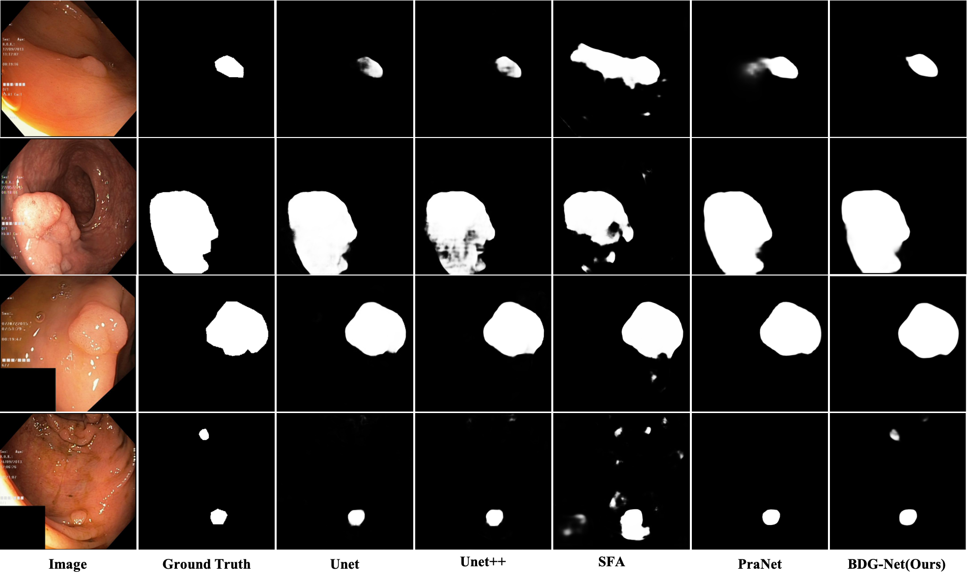
As shown in Table 1, our model obtains mean-Dice of 0.915 and mean-IoU of 0.865 on Kavsir dataset. Other metrics are also better than previous methods remarkably, which shows that our model outperforms all previous state-of-the-art methods. In addition, we calculate the FLOPs under the 352352 input resolution, and our model achieves the lowest FLOPs, which indicates that our model has the fastest inference speed and lowest computational complexity. As shown in Table 2, our model outperforms all other methods on the CVC-ClinicDB dataset as well. The visual results on Figure 5 also show the superiority of our BDG-Net over previous methods. Our method improves the polyps segmentation significantly, especially on smaller objects and unclear boundaries.
| Methods | mean Dice | mean IoU | MAE | FLOPs(G) | |||
| U-Net[3] (MICCAI’15) | 0.818 | 0.746 | 0.794 | 0.858 | 0.893 | 0.055 | 25.965 |
| U-Net++[5] (TMI’19) | 0.821 | 0.743 | 0.808 | 0.862 | 0.910 | 0.048 | 65.925 |
| ResUNet-mod[16] | 0.791 | n/a | n/a | n/a | n/a | n/a | n/a |
| ResUNet++[17] | 0.813 | 0.793 | n/a | n/a | n/a | n/a | 134.109 |
| SFA[18] (MICCAI’19) | 0.723 | 0.611 | 0.670 | 0.782 | 0.849 | 0.075 | n/a |
| PraNet[6] (MICCAI’20) | 0.898 | 0.840 | 0.885 | 0.915 | 0.948 | 0.030 | 13.078 |
| BDG-Net (Ours) | 0.915 | 0.865 | 0.906 | 0.923 | 0.972 | 0.021 | 10.840 |
To verify the generalization ability of our model, we test on three unseen datasets, including CVC-ColonDB, ETIS, and CVC300. The experimental results show that the proposed method achieves much higher performance than other methods, which reveals the excellent generalization ability of our model.
| Methods | CVC-ClinicDB | ColonDB | ETIS | CVC300 |
| mDice mIoU | mDice mIoU | mDice mIoU | mDice mIoU | |
| U-Net[3] (MICCAI’15) | 0.823 0.755 | 0.512 0.444 | 0.398 0.335 | 0.710 0.627 |
| U-Net++[5] (TMI’19) | 0.794 0.729 | 0.483 0.410 | 0.401 0.344 | 0.707 0.624 |
| SFA[18] (MICCAI’19) | 0.700 0.607 | 0.469 0.347 | 0.297 0.217 | 0.467 0.329 |
| PraNet[6] (MICCAI’20) | 0.899 0.849 | 0.709 0.640 | 0.628 0.567 | 0.871 0.797 |
| BDG-Net (Ours) | 0.916 0.864 | 0.804 0.725 | 0.756 0.679 | 0.899 0.831 |
3.3 Ablation Studies
In this section, We conduct exhaustive ablation study to evaluate the contribution of each component for our BDG-Net. We also investigate the number of skip path and the selection of .
3.3.1 Effect of BDGM and BDGD
From Table 3, we can observe that Row No.2 (Backbone + BDGM) outperforms Row No.1 (Backbone), where mean Dice has increased by 1.1%. Besides, We can also observe that the performance of Row No.3 is significantly better than that of Row No.1 (backbone), increasing the mean Dice and mean IoU by 2.6%, 3.9% respectively. To study whether the combination of BDGM and BDGD contributes, Row No.4 (Backbone + BDGM + BDGD) shows the highest performance towards all other settings (No.1 No.3), which improves mean Dice and mean IoU to 0.915 and 0.865, respectively.
| Setting | mean Dice | mean IoU |
| Backbone | 0.859 | 0.780 |
| Backbone + BDGM | 0.870 | 0.796 |
| Backbone + BDGD | 0.896 | 0.835 |
| Backbone + BDGM + BDGD | 0.915 | 0.865 |
3.3.2 Number of Skip Path and the Choice of
As shown in Table 4, we can achieve the best result when only using the third and fourth levels of encoder features. Since low-level features are primarily spatial features with much noise, fusing with the first and second-level of encoder features does not bring any gain. We also test the selection of . The experimental results show that when the skip path is employed at the third and fourth stages, the of 5 can achieve the best results.
| Feature Level | ||||
| 4 | 0.911 | 0.912 | 0.911 | 0.906 |
| 3, 4 | 0.906 | 0.910 | 0.915 | 0.911 |
| 2, 3, 4 | 0.908 | 0.909 | 0.908 | 0.910 |
| 1, 2, 3, 4 | 0.912 | 0.906 | 0.903 | 0.906 |
 |
4 Conclusions
In this paper, we present a novel architecture, BDG-Net, for accurate polyp segmentation from colonoscopy images. BDG-Net consists of two novel modules, namely BDGM and BDGD. BDGM generates BDM to estimate the boundary distribution of polyps. Then, the generated BDM is passed to BDGD to guide the polyp segmentation. Extensive experiments demonstrate that the BDG-Net consistently outperforms all state-of-the-art methods across five challenging datasets on six metrics while maintaining the lowest computational complexity.
Acknowledgements.
This work was supported in part by the National Natural Science Foundation of China under Grant 62071086 and Sichuan Science and Technology Program under Grant 2021YFG0296.References
- [1] Jha, D., Smedsrud, P. H., Riegler, M. A., Halvorsen, P., de Lange, T., Johansen, D., and Johansen, H. D., “Kvasir-seg: A segmented polyp dataset,” in [International Conference on Multimedia Modeling ], 451–462, Springer (2020).
- [2] Silva, J., Histace, A., Romain, O., Dray, X., and Granado, B., “Toward embedded detection of polyps in wce images for early diagnosis of colorectal cancer,” International journal of computer assisted radiology and surgery 9(2), 283–293 (2014).
- [3] Ronneberger, O., Fischer, P., and Brox, T., “U-net: Convolutional networks for biomedical image segmentation,” in [International Conference on Medical image computing and computer-assisted intervention ], 234–241, Springer (2015).
- [4] Oktay, O., Schlemper, J., Folgoc, L. L., Lee, M., Heinrich, M., Misawa, K., Mori, K., McDonagh, S., Hammerla, N. Y., Kainz, B., et al., “Attention u-net: Learning where to look for the pancreas,” arXiv preprint arXiv:1804.03999 (2018).
- [5] Zhou, Z., Siddiquee, M. M. R., Tajbakhsh, N., and Liang, J., “Unet++: A nested u-net architecture for medical image segmentation,” in [Deep learning in medical image analysis and multimodal learning for clinical decision support ], 3–11, Springer (2018).
- [6] Fan, D.-P., Ji, G.-P., Zhou, T., Chen, G., Fu, H., Shen, J., and Shao, L., “Pranet: Parallel reverse attention network for polyp segmentation,” in [International Conference on Medical Image Computing and Computer-Assisted Intervention ], 263–273, Springer (2020).
- [7] Liu, S., Huang, D., et al., “Receptive field block net for accurate and fast object detection,” in [Proceedings of the European Conference on Computer Vision (ECCV) ], 385–400 (2018).
- [8] Tan, M. and Le, Q., “Efficientnet: Rethinking model scaling for convolutional neural networks,” in [International Conference on Machine Learning ], 6105–6114, PMLR (2019).
- [9] Bernal, J., Sánchez, F. J., Fernández-Esparrach, G., Gil, D., Rodríguez, C., and Vilariño, F., “Wm-dova maps for accurate polyp highlighting in colonoscopy: Validation vs. saliency maps from physicians,” Computerized Medical Imaging and Graphics 43, 99–111 (2015).
- [10] Tajbakhsh, N., Gurudu, S. R., and Liang, J., “Automated polyp detection in colonoscopy videos using shape and context information,” IEEE transactions on medical imaging 35(2), 630–644 (2015).
- [11] Vázquez, D., Bernal, J., Sánchez, F. J., Fernández-Esparrach, G., López, A. M., Romero, A., Drozdzal, M., and Courville, A., “A benchmark for endoluminal scene segmentation of colonoscopy images,” Journal of healthcare engineering 2017 (2017).
- [12] Margolin, R., Zelnik-Manor, L., and Tal, A., “How to evaluate foreground maps?,” in [Proceedings of the IEEE conference on computer vision and pattern recognition ], 248–255 (2014).
- [13] Fan, D.-P., Cheng, M.-M., Liu, Y., Li, T., and Borji, A., “Structure-measure: A new way to evaluate foreground maps,” in [Proceedings of the IEEE international conference on computer vision ], 4548–4557 (2017).
- [14] Fan, D.-P., Gong, C., Cao, Y., Ren, B., Cheng, M.-M., and Borji, A., “Enhanced-alignment measure for binary foreground map evaluation,” arXiv preprint arXiv:1805.10421 (2018).
- [15] Perazzi, F., Krähenbühl, P., Pritch, Y., and Hornung, A., “Saliency filters: Contrast based filtering for salient region detection,” in [2012 IEEE conference on computer vision and pattern recognition ], 733–740, IEEE (2012).
- [16] Zhang, Z., Liu, Q., and Wang, Y., “Road extraction by deep residual u-net,” IEEE Geoscience and Remote Sensing Letters 15(5), 749–753 (2018).
- [17] Jha, D., Smedsrud, P. H., Riegler, M. A., Johansen, D., De Lange, T., Halvorsen, P., and Johansen, H. D., “Resunet++: An advanced architecture for medical image segmentation,” in [2019 IEEE International Symposium on Multimedia (ISM) ], 225–2255, IEEE (2019).
- [18] Fang, Y., Chen, C., Yuan, Y., and Tong, K.-y., “Selective feature aggregation network with area-boundary constraints for polyp segmentation,” in [International Conference on Medical Image Computing and Computer-Assisted Intervention ], 302–310, Springer (2019).